
Electromagnetic form factors of the...
144
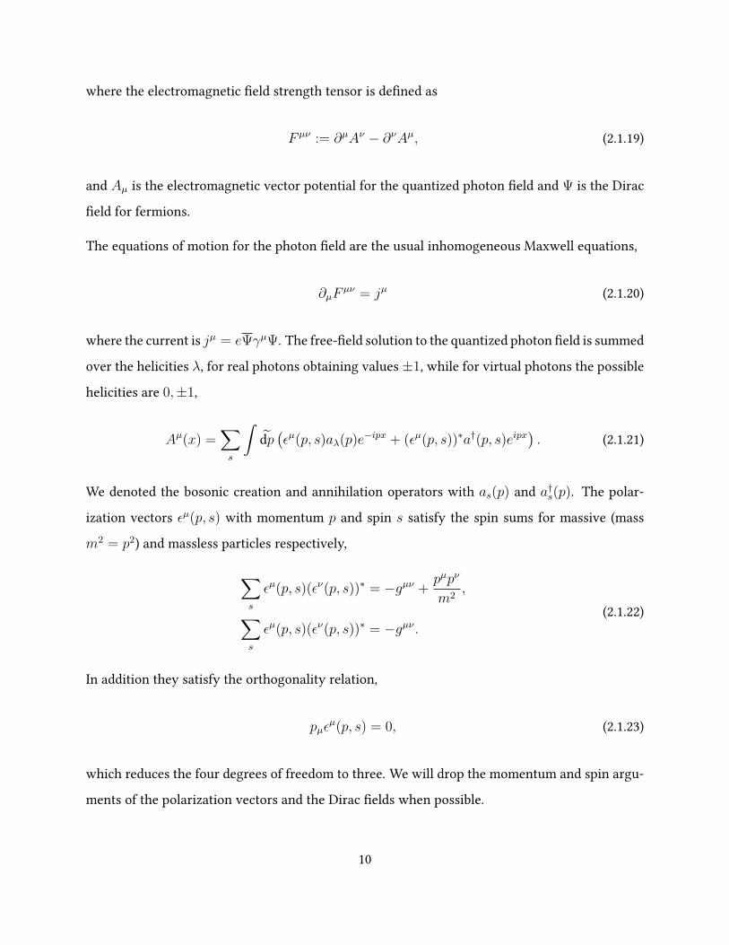
U U D P A D N P Electromagnetic form factors of the Σ * - Λ transition Master Degree Project Author: Timea Vitos Supervisor: Stefan Leupold Subject reader : Karin Schönning September 1, 2019
Transcript of Electromagnetic form factors of the...
Uppsala University
Department of Physics and Astronomy
Division of Nuclear Physics
Electromagnetic form factors of
the Σ∗ − Λ transition
Master Degree Project
Author:
Timea Vitos
Supervisor:
Stefan Leupold
Subject reader :
Karin Schönning
September 1, 2019
Abstract
We introduce and examine the analytic properties of the three electromagnetic transition form
factors of the Σ∗-Λ hyperon transition. In the rst part of the thesis, we discuss the interaction
Lagrangian for the hyperons at hand. We calculate the decay rate of the Dalitz decay Σ∗ → Λe+e−
in the one-photon approximation in terms of the form factors, as well as the dierential cross
section of the scattering e+e− → Σ∗Λ in the one-photon approximation. In the second part
of the thesis, we build up the machinery for calculation of the form factors using dispersion
relations, performing an analytic continuation from the timelike, q2 > 0, to the spacelike, q2 < 0,
region of the virtual photon invariant mass q2. Due to an anomalous cut in the triangle diagram
arising from a two-pion saturation of the photon-hyperon vertex, there is an additional term in
the dispersive integral. We use the scalar three-point function as a model for the examination
of the dispersive approach with the anomalous cut. The one-loop diagram is calculated both
directly and using dispersion relations. After comparison of the two methods, they are found to
coincide when the anomalous contribution is added to the dispersive integral in the case of the
octet Σ exchange. By examination of the branch points of the logarithm in the discontinuity,
we deduce the structure of the Riemann surface of the unitarity cut and present trajectories of
the branch points. The result of our analysis of the analytic structure yields a correct dispersive
relation for the electromagnetic transition form factors. This opens the way for the calculation
of these form factors in the low-energy region for both space- and timelike q2. As an outlook, we
present preliminary calculations for the hyperon-pion scattering amplitude using the unitarity
and the anomalous contribution in a once-subtracted dispersion relation. Finally we present the
corresponding preliminary unsubtracted dispersive calculations for the form factors.
i

Acknowledgments
My greatest gratitude is in part towards my supervisor Stefan Leupold, who has introduced me
to the subject of theoretical particle physics. I thank him for his patience with my questions; for
his help with the physics and numerical calculations; and for our interesting discussions. In other
part, my gratitude is towards my co-supervisor Elisabetta Perotti, who has been my companion
in this journey through this thesis. I thank her for her support in this work, and also in life during
this period which showed challenges and diculties.
My further thanks is to the Divisions of Nuclear Physics and High Energy Physics with whom
we shared kitchen, for the pleasant company at work, lunch and breaks. With the familiar atmo-
sphere present in this part of the Ångström laboratory, it was a real joy spending long days at
work.
I thank my friends in all parts of the world, whom I could laugh and travel with, and who gave
me valuable feedback on this project and the progress of writing it. Most importantly, I thank my
parents and sister Noemi who have been a base of comfort in times when work was dicult and
a magnier of happiness at times when work was successful.
ii
Populärvetenskaplig sammanfattning
Det mesta av den observerade materian i vårt universum består av protoner och neutroner, de
partiklar som tillsammans bildar atomkärnor i atomerna. Protoner och neutroner är däremot inte
fundamentala partiklar: de består i sin tur av kvarkar och gluoner. Den bästa teoretiska modellen
som vi har idag för att beskriva partiklar är standardmodellen. I denna kvantfältteori beskrivs
partiklar som fält i rumtiden. Det nns däremot mycket som fortfarande måste ges svar på inom
standardmodellen. En av dessa är kvarkarnas egenskap att vara fast knutna till de sammansatta
partiklar som de bildar, hadronerna, vid låga energier. Detta fenomen kräver mer kunskap om
den starka växelverkan, den kraft som håller kvarkar och gluoner ihop.
För att undersöka kvarkarnas och den starka växelverkans natur kan man undersöka de två lät-
taste kvarkar som förekommer som stabila partiklar inuti protoner och neutroner: u- och d-
kvarkarna. Med partikelacceleratorer kan vi få tillgång till även instabila hadroner, som in-
nehåller andra, tyngre kvarkar, som s-kvarken. Genom att undersöka naturen hos sådana ex-
otiska hadroner, kan vi få ut kunskap om den fundamentala starka växelverkan.
I denna avhandling undersöks Σ∗ till Λ övergången. Båda partiklar är hadroner med uds kvark-
sammansättningen. Då kvarkar är elektriskt laddade partiklar, växelverkar de även genom den
elektromagnetiska växelverkan, vilket är den kraft som driver denna specika övergång. Med
eektiv fältteori kan vi undersöka denna övergång genom att betrakta partiklarna som punk-
tformiga. De så kallade formfaktorer som övergången parametriseras av, är funktioner som
beskriver den inneboende egenskaperna av hadronerna.
Formfaktorer kan för vissa energier bestämmas med experiment. De energiintervall som behövs
för att tolka formfaktorer som fysikaliska egenskaper av hadroner kan däremot för dessa speci-
ka partiklar inte mätas i dagsläget. Man kan däremot få tillgång till dessa energiintervall genom
dispersiva integraler, som tar funktioner från ett intervall till ett annat. På grund av relationerna
mellan massorna av dessa hadroner, nns en tekniskt knepig aspekt till dispersiva beräkningarna.
Detta är den så kallade anomaliska gränsen, som förekommer i integralerna som en extra term.
För att undersöka hur detta fungerar på de riktiga formfaktorer, används i denna avhandling
iii
det skalära diagrammet som en modell för att undersöka dispersiva relationerna. Vi presen-
terar resultatet av det skalära diagrammet, både med en explicit beräkning, samt med dispersiva
beräkningar. Dessa jämförs för att klarlägga hur den anomaliska gränsen ska inkluderas i disper-
siva beräkningarna. Genom att undersöka hur dispersiva beräkningarna fungerar på det skalära
diagrammet, öppnar vi porten till beräkningarna till formfaktorerna. I avhandlingen presenteras
preliminära resultat för dispersiva beräkningar av formfaktorerna.
iv
Contents
Abstract i
Acknowledgments ii
Populärvetenskaplig sammanfattning iii
1 Introduction 1
1.1 Outline . . . . . . . . . . . . . . . . . . . . . . . . . . . . . . . . . . . . . . . . . . 3
2 Brief theory background 5
2.1 Quantum elds and Lagrangians . . . . . . . . . . . . . . . . . . . . . . . . . . . . 5
2.1.1 Spin-12
Dirac elds . . . . . . . . . . . . . . . . . . . . . . . . . . . . . . . 5
2.1.2 Quantum electrodynamics . . . . . . . . . . . . . . . . . . . . . . . . . . . 9
2.1.3 Spin-32
elds . . . . . . . . . . . . . . . . . . . . . . . . . . . . . . . . . . . 11
2.1.4 Baryons and mesons . . . . . . . . . . . . . . . . . . . . . . . . . . . . . . 12
2.1.5 Symmetries . . . . . . . . . . . . . . . . . . . . . . . . . . . . . . . . . . . 13
2.2 Eective eld theories . . . . . . . . . . . . . . . . . . . . . . . . . . . . . . . . . . 17
2.2.1 Chiral perturbation theory . . . . . . . . . . . . . . . . . . . . . . . . . . . 18
2.2.2 Vertex functions and form factors . . . . . . . . . . . . . . . . . . . . . . . 19
2.3 Scattering theory . . . . . . . . . . . . . . . . . . . . . . . . . . . . . . . . . . . . 21
2.4 The Σ∗-Λ transition . . . . . . . . . . . . . . . . . . . . . . . . . . . . . . . . . . . 23
3 Feynman rules 25
v
3.1 Parity transformation of vertex function . . . . . . . . . . . . . . . . . . . . . . . 26
3.2 Vertex function and form factors . . . . . . . . . . . . . . . . . . . . . . . . . . . . 28
3.3 Hyperon interaction Lagrangian . . . . . . . . . . . . . . . . . . . . . . . . . . . . 36
4 Cross section and decay rate 46
4.1 Cross section of e+e− → Σ∗Λ . . . . . . . . . . . . . . . . . . . . . . . . . . . . . 47
4.2 Decay rate of Σ∗ → Λe+e− . . . . . . . . . . . . . . . . . . . . . . . . . . . . . . . 55
4.3 Decay rate of Σ∗ → Λγ . . . . . . . . . . . . . . . . . . . . . . . . . . . . . . . . . 60
5 Anomalous cut of the scalar triangle diagram 62
5.1 Prerequisites and denitions . . . . . . . . . . . . . . . . . . . . . . . . . . . . . . 63
5.1.1 Dispersion relations . . . . . . . . . . . . . . . . . . . . . . . . . . . . . . 63
5.1.2 Cutkosky cutting rules . . . . . . . . . . . . . . . . . . . . . . . . . . . . . 66
5.1.3 Riemann surfaces and cuts . . . . . . . . . . . . . . . . . . . . . . . . . . . 68
5.1.4 Exchange states in the two-pion one-loop diagram . . . . . . . . . . . . . 69
5.2 Direct loop calculation . . . . . . . . . . . . . . . . . . . . . . . . . . . . . . . . . 72
5.3 Analytic properties along the unitarity cut . . . . . . . . . . . . . . . . . . . . . . 80
5.3.1 Discontinuity along the unitarity cut . . . . . . . . . . . . . . . . . . . . . 81
5.3.2 Riemann sheets of the unitarity cut . . . . . . . . . . . . . . . . . . . . . . 85
5.4 Dispersive calculations . . . . . . . . . . . . . . . . . . . . . . . . . . . . . . . . . 88
5.4.1 Branch points of the discontinuity . . . . . . . . . . . . . . . . . . . . . . 88
5.4.2 Dispersion relation with anomalous discontinuity . . . . . . . . . . . . . . 92
5.4.3 Decuplet exchange, mex = mΣ∗ . . . . . . . . . . . . . . . . . . . . . . . . 95
5.4.4 Octet exchange, mex = mΣ . . . . . . . . . . . . . . . . . . . . . . . . . . 99
6 Dispersion relations for the transition form factors 104
6.1 Omnès function and pion phase shift . . . . . . . . . . . . . . . . . . . . . . . . . 107
6.2 Dispersion relations for Tm(s) . . . . . . . . . . . . . . . . . . . . . . . . . . . . . 109
6.3 Dispersion relations for Gm(s) . . . . . . . . . . . . . . . . . . . . . . . . . . . . . 117
vi
7 Conclusions and outlook 122
Appendices 124
A Vector spinors 125
B Interaction Lagrangians 127
C Omnès solution 129
D Amplitude functions 131
Bibliography 132
vii
Chapter 1
Introduction
The Standard Model (SM) comprises currently our best understanding of fundamental and com-
posite particles. Quantum chromodynamics (QCD) describes the strong interaction, which is the
interaction between the quarks inside hadrons. The main part of the observed mass in our uni-
verse is composed of nucleons: protons and neutrons. On the scale of particle physics, both of
these hadrons are stable as single entities and they form the stable nuclei of atoms. The SU(3)
avor symmetry of QCD suggests that a change of a u or d quark with the next lightest quark,
the strange quark, may produce particles closely related to the stable nucleons. This motivates
the study of hyperons, which are hadrons with a heavier quark.
At very high energies, due to the running of the strong coupling, quarks behave as almost free par-
ticles. This phenomenon is named asymptotic freedom and was one of the biggest breakthroughs
of modern particle physics. At low energies, quarks are conned into hadrons, a phenomenon
named connement and one that still is one of the biggest unsolved questions in particle physics.
At low energies, the relevant degrees of freedom are no longer the quarks, which up to today we
consider fundamental particles, but instead the hadrons. This idea leads to eective eld theories,
which is the reduction of a more underlying microscopic model to one which includes only the
scale of interest.
The main interest remains even in the eective eld theory approach to be the properties of
1
quarks and the underlying interactions. This is taken into considerations by form factors [1].
Form factors parametrize the structure of hadrons and relate to observables which can be directly
measured. Form factors are functions of the transferred momentum in an interaction between
hadrons. The exact shape of the form factor is unique to the hadrons considered and the mediating
interaction. In this thesis, we consider the electromagnetic form factors of the transition between
the rst excitation of the Σ particle, the Σ∗ particle, to the Λ particle. The transition is driven by
the electromagnetic interaction, in which case the transferred momentum is carried by virtual
photons.
In the thesis we are concerned with the one-photon approximation, in which case the form factors
are functions of the invariant mass q2 of the virtual photon. The physical interpretation of the
form factors as the electric and magnetic radii is valid for form factors in the region of spacelike
q2. Form factors in the spacelike region can be obtained with xed-target experiments, for a
collision of an electron with a hyperon. In the case of unstable hyperons, however, this at present
is not a feasible experiment. The form factors can however be obtained in the timelike region
by other reactions, such as the Dalitz decay Σ∗ → Λe+e− and the electron-positron scattering
e+e− → Σ∗Λ. By assumption that the form factors are analytic functions of the invariant mass,
these can be analytically continued from the timelike region to the spacelike. This is done with
dispersion relations, which is the objective of the second part of this thesis.
Dispersion relations allow to obtain an analytic function by an integral over the discontinuity
of the function. At low energies the non-trivial structure of the form factors emerges from the
lowest-mass excited pseudo-scalar Goldstone bosons, being the two-pion intermediate state. This
intermediate state relates the form factors to hyperon-pion scattering amplitudes. In turn, these
amplitudes receive contributions from the exchange of hyperons. For a dispersive representation
of a form factor, the standard procedure is an integral over the two-pion unitarity cut. For the
previously studied Σ-Λ electromagnetic form factors [2], the discontinuity of the form factors
includes a unitarity cut only. In the case of the Σ∗-Λ, an additional cut is expected due to the
heavier mass of the decuplet hyperon Σ∗ compared to the octet hyperon Σ. Thus, the dispersive
relations acquire an additional anomalous contribution. The analytic structure of the diagram
2
can be examined by considering the simpler, scalar loop case, for which we can exactly calculate
the diagram. Also for this diagram, dispersion relations can be formulated and examined when
the anomalous piece is needed. Thus, by comparison to the exact result for the case of the scalar
triangle diagram, one can pin down the correct dispersive representation for the hyperon transi-
tion form factors. This analysis provides the key for the correct calculation of the form factors in
terms of hyperon-pion scattering amplitudes. The main part of the thesis comprises the analysis
of dispersive approach to the calculation of the scalar triangle diagram. In addition, preliminary
results for the calculation of the electromagnetic form factors are presented, which is the project
in progress to which the work of this thesis contributes, and is planned to be presented by Junker,
Leupold, Perotti and Vitos [3].
1.1 Outline
This thesis consists of two main parts. The rst half presents the form factors, the interaction
terms in the Lagrangian and Feynman rules for this interaction. The second part considers the
dispersion relations for the form factors, and their analytic structure.
In Chapter 2, we dene the essential ingredients from quantum eld theory in order to put the
topic into context and to clarify the conventions. The statements in this chapter are fully based
on previously laid fundamental works in quantum eld theory, well established in the physics
community. This part is included for completeness and easy reading and understanding of the
rest of the thesis. In Chapter 3, we consider the interaction Lagrangian for the hyperons Σ∗ and
Λ. We construct the current and the vertex function in terms of the form factors. The method
in this chapter is not unique and has been performed for other Lagrangians by previous authors,
however for the present interaction, the author of this thesis, based on discussions with supervi-
sor Leupold, performed the step-by-step construction. In Chapter 4, we present the calculations
for the decay rate and the scattering cross section for the two reactions in which the form factors
can be measured at present and in the near future. The work in this chapter is based on direct
calculations by the author of the thesis, and cross-checks with co-supervisor Perotti. In Chapter
3
5, we use the scalar triangle diagram as a model to examine the analytic structure of the triangle
diagram with the two-pion exchange. The analysis for the scalar triangle diagram is done both
when the anomalous cut must be omitted and when it must be included. The work in this chap-
ter is the main part of the individual work performed by the author of this thesis, strengthened
by discussions and cross-checks with both supervisors Leupold and Perotti. Chapter 6 contains
preliminary results for the dispersion relations for the form factors. The preliminary results are
performed by the author of the thesis, while the method is based on that used previously by
Granados, Leupold and Perotti in the previous work of the Σ-Λ electromagnetic transition form
factors [2].
4
Chapter 2
Brief theory background
In this chapter we recall some of the main features of quantum eld theory which are needed in
the rst part of the thesis. For more details and thorough derivations, we refer to Srednicki [4],
Peskin and Schroeder [5] and Weinberg [6], as well as many other basic textbooks in quantum
eld theory. Throughout the thesis we use natural units, in which we set c = ~ = 1.
2.1 Quantum elds and Lagrangians
We rstly introduce Dirac elds, which are elds with spin. In this work, the hadrons considered
are spin-12
and spin-32
elds, and are thus Dirac elds. We then introduce the main parts of quan-
tum electrodynamics needed to treat these elds in the interaction Lagrangian and in calculating
the cross section and decay rates. We include the relevant information on the lightest baryons
and mesons in the baryon octet and baryon decuplet and the meson octet.
2.1.1 Spin-12 Dirac elds
Spin- 12
fermions are described by Dirac spinors Ψ, being objects consisting of a left- and a right-
handed representation of the Lorentz group. The free Dirac Lagrangian is written in the Lorentz
5
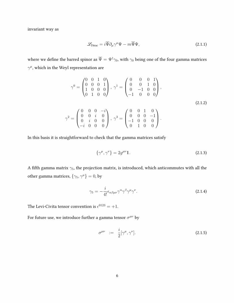
invariant way as
LDirac = iΨ∂µγµΨ−mΨΨ, (2.1.1)
where we dene the barred spinor as Ψ = Ψ†γ0, with γ0 being one of the four gamma matrices
γµ, which in the Weyl representation are
γ0 =
0 0 1 00 0 0 11 0 0 00 1 0 0
, γ1 =
0 0 0 10 0 1 00 −1 0 0−1 0 0 0
,
γ2 =
0 0 0 −i0 0 i 00 i 0 0−i 0 0 0
, γ3 =
0 0 1 00 0 0 −1−1 0 0 00 1 0 0
.
(2.1.2)
In this basis it is straightforward to check that the gamma matrices satisfy
γµ, γν = 2gµν1. (2.1.3)
A fth gamma matrix γ5, the projection matrix, is introduced, which anticommutes with all the
other gamma matrices, γ5, γµ = 0, by
γ5 = − i
4!εαβµνγ
αγβγµγν . (2.1.4)
The Levi-Civita tensor convention is ε0123 = +1.
For future use, we introduce further a gamma tensor σµν by
σµν :=i
2[γµ, γν ]. (2.1.5)
6
The equation of motion of the Dirac Lagrangian is the Dirac equation,
(i/∂ −m)Ψ(x) = 0, (2.1.6)
with a Dirac eld with momentum pµ = (E,p) and E =√|p|2 +m2. The solution to this equa-
tion is given by the spin-summed expansion in terms of the annihilation operators as(p), bs(p)
and creation operators a†s(p), b†s(p) acting in the Fock space, and spinor structures u(p, s), v(p, s),
as well as the free-wave propagation part e±ipx,
Ψ(x) =∑s
∫dp(as(p)u(p, s)e−ipx + b†s(p)v(p, s)eipx
),
Ψ(x) =∑s
∫dp(a†s(p)u(p, s)eipx + bs(p)v(p, s)e−ipx
),
(2.1.7)
summed over all possible spin polarizations s, with the Lorentz invariant normalized spatial dif-
ferential,
dp :=d3p
(2π)32E, (2.1.8)
and the barred spinors
u(p, s) := u†(p, s)γ0,
v(p, s) := v†(p, s)γ0.(2.1.9)
The spin-12
spinors satisfy the spin sums
∑s
u(p, s)u(p, s) = (/p+m),
∑s
v(p, s)v(p, s) = (/p−m),(2.1.10)
7
and the equations (referred to as Dirac equations for spinors)
(−/p+m)u(p, s) = 0,
v(p, s)(/p+m) = 0.(2.1.11)
These solutions (2.1.7) and (2.1.11) can be inverted to obtain the ladder operators in terms of the
spinor elds,
as(p) =
∫d3x e−ipxu(p, s)γ0Ψ(x),
a†s(p) =
∫d3x eipxΨ(x)γ0u(p, s),
b†s(p) =
∫d3x eipxv(p, s)γ0Ψ(x),
bs(p) =
∫d3x e−ipxΨ(x)γ0v(p, s).
(2.1.12)
After quantizing the elds, these coecients get promoted to operators, and satisfy then the
anticommutation relations (and the corresponding commutation relations for bosonic elds),
as(p), as′(p′) = a†s(p), a†s′(p′) = 0,
as(p), a†s′(p′) = (2π)32Eδss′δ(3)(p− p′),
(2.1.13)
with all other anticommutators vanishing. The vacuum state is constructed so that it is annihi-
lated by the annihilation operators
as(p) |0〉 = bs(p) |0〉 = 0. (2.1.14)
A single-particle state with momentum p and spin s is given by the action of the creation operator
of the corresponding eld on the vacuum state,
|(p, s)〉 = a†s(p) |0〉 ,
〈(p, s)| = |(p, s)〉† = 〈0| as(p).(2.1.15)
8
Correspondingly, an n-particle and m-antiparticle state is produced by the action of the ladder
operators with corresponding momentum and spin in the corresponding order,
|(p1, s1), ..., (pn, sn); (p′1, s′1), ..., (p′m, s
′m)〉 = a†s1(p1)...a†sn(pn)b†s′1
(p′1)...b†s′m(p′m) |0〉 . (2.1.16)
The states are normalized as
〈(p, s)|(p′, s′)〉 = (2π)32Eδss′δ(3)(p− p′), (2.1.17)
with E =√|p|2 +m2. The normalization implies that any two states with dierent momenta
and spins are orthogonal.
In this work we consider hyperon states in the low-energy limit, where the degrees of freedom are
the hyperons themselves. Often we will refer to helicity instead of spin. Helicity is the projection
of the spin on the direction of motion. We will, in general, suppress the spin or helicity argument
in the creation and annihilation operators and the states.
2.1.2 Quantum electrodynamics
Before proceeding to present the spin-32
vector-spinor Dirac elds, we rst introduce the most im-
portant bits of the quantized theory of the electromagnetic interaction, where we also introduce
the polarization vector, which is needed for the construction of the vector-spinor elds.
The electromagnetic form factors parametrize the hadron structure in the electromagnetic inter-
action. The probing of hadrons occurs with electrons. For the pointlike electron-photon interac-
tions, we use perturbative expansion in the ne structure constant (or equivalently the electric
charge). For this we need to now introduce the quantum eld theory for the electromagnetic in-
teraction, quantum electrodynamics (QED). For a theory of interacting fermions, the spinor QED
Lagrangian takes the form
LQED = −1
4FµνF
µν + Ψ(i/∂ −m)Ψ + eAµΨγµΨ, (2.1.18)
9
where the electromagnetic eld strength tensor is dened as
F µν := ∂µAν − ∂νAµ, (2.1.19)
and Aµ is the electromagnetic vector potential for the quantized photon eld and Ψ is the Dirac
eld for fermions.
The equations of motion for the photon eld are the usual inhomogeneous Maxwell equations,
∂µFµν = jµ (2.1.20)
where the current is jµ = eΨγµΨ. The free-eld solution to the quantized photon eld is summed
over the helicities λ, for real photons obtaining values ±1, while for virtual photons the possible
helicities are 0,±1,
Aµ(x) =∑s
∫dp(εµ(p, s)aλ(p)e
−ipx + (εµ(p, s))∗a†(p, s)eipx). (2.1.21)
We denoted the bosonic creation and annihilation operators with as(p) and a†s(p). The polar-
ization vectors εµ(p, s) with momentum p and spin s satisfy the spin sums for massive (mass
m2 = p2) and massless particles respectively,
∑s
εµ(p, s)(εν(p, s))∗ = −gµν +pµpν
m2,
∑s
εµ(p, s)(εν(p, s))∗ = −gµν .(2.1.22)
In addition they satisfy the orthogonality relation,
pµεµ(p, s) = 0, (2.1.23)
which reduces the four degrees of freedom to three. We will drop the momentum and spin argu-
ments of the polarization vectors and the Dirac elds when possible.
10
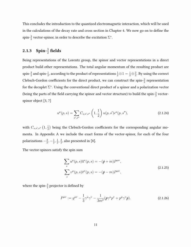
This concludes the introduction to the quantized electromagnetic interaction, which will be used
in the calculations of the decay rate and cross section in Chapter 4. We now go on to dene the
spin-32
vector-spinor, in order to describe the excitation Σ∗.
2.1.3 Spin-32 elds
Being representations of the Lorentz group, the spinor and vector representations in a direct
product build other representations. The total angular momentum of the resulting product are
spin-32
and spin-12, according to the product of representations 1
2⊗1 = 1
2⊕ 3
2. By using the correct
Clebsch-Gordon coecients for the direct product, we can construct the spin-32
representation
for the decuplet Σ∗. Using the conventional direct product of a spinor and a polarization vector
(being the parts of the eld carrying the spinor and vector structure) to build the spin-32
vector-
spinor object [3, 7]
uµ(p, s) =∑s′,s′′
Cs,s′,s′′
(1,
1
2
)u(p, s′)εµ(p, s′′), (2.1.24)
with Cs,s′,s′′(1, 1
2
)being the Clebsch-Gordon coecients for the corresponding angular mo-
menta. In Appendix A we include the exact forms of the vector-spinor, for each of the four
polarizations −32,−1
2, 1
2, 3
2, also presented in [8].
The vector-spinors satisfy the spin sum
∑s
uµ(p, s)uν(p, s) = −(/p+m)P µν ,
∑s
vµ(p, s)vν(p, s) = −(/p−m)P µν ,(2.1.25)
where the spin-32
projector is dened by
P µν := gµν − 1
3γµγν − 1
3m2(/pγ
µpν + pµγν/p). (2.1.26)
11
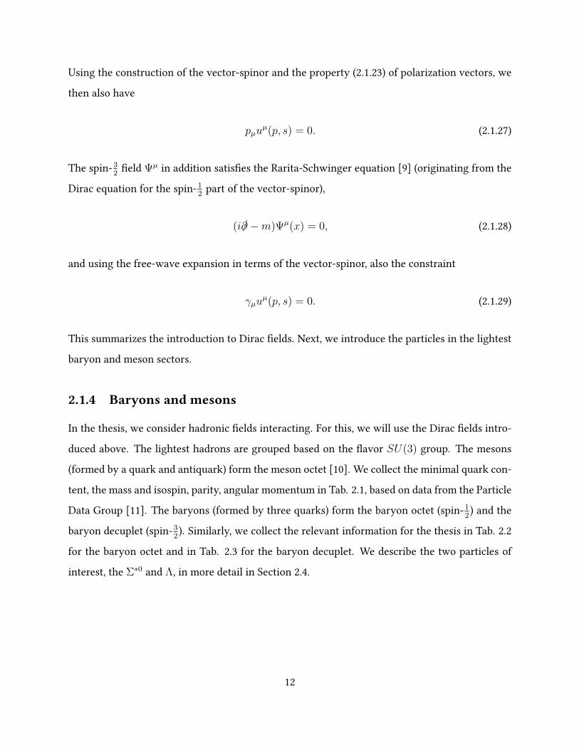
Using the construction of the vector-spinor and the property (2.1.23) of polarization vectors, we
then also have
pµuµ(p, s) = 0. (2.1.27)
The spin-32
eld Ψµ in addition satises the Rarita-Schwinger equation [9] (originating from the
Dirac equation for the spin-12
part of the vector-spinor),
(i/∂ −m)Ψµ(x) = 0, (2.1.28)
and using the free-wave expansion in terms of the vector-spinor, also the constraint
γµuµ(p, s) = 0. (2.1.29)
This summarizes the introduction to Dirac elds. Next, we introduce the particles in the lightest
baryon and meson sectors.
2.1.4 Baryons and mesons
In the thesis, we consider hadronic elds interacting. For this, we will use the Dirac elds intro-
duced above. The lightest hadrons are grouped based on the avor SU(3) group. The mesons
(formed by a quark and antiquark) form the meson octet [10]. We collect the minimal quark con-
tent, the mass and isospin, parity, angular momentum in Tab. 2.1, based on data from the Particle
Data Group [11]. The baryons (formed by three quarks) form the baryon octet (spin-12) and the
baryon decuplet (spin-32). Similarly, we collect the relevant information for the thesis in Tab. 2.2
for the baryon octet and in Tab. 2.3 for the baryon decuplet. We describe the two particles of
interest, the Σ∗0 and Λ, in more detail in Section 2.4.
12
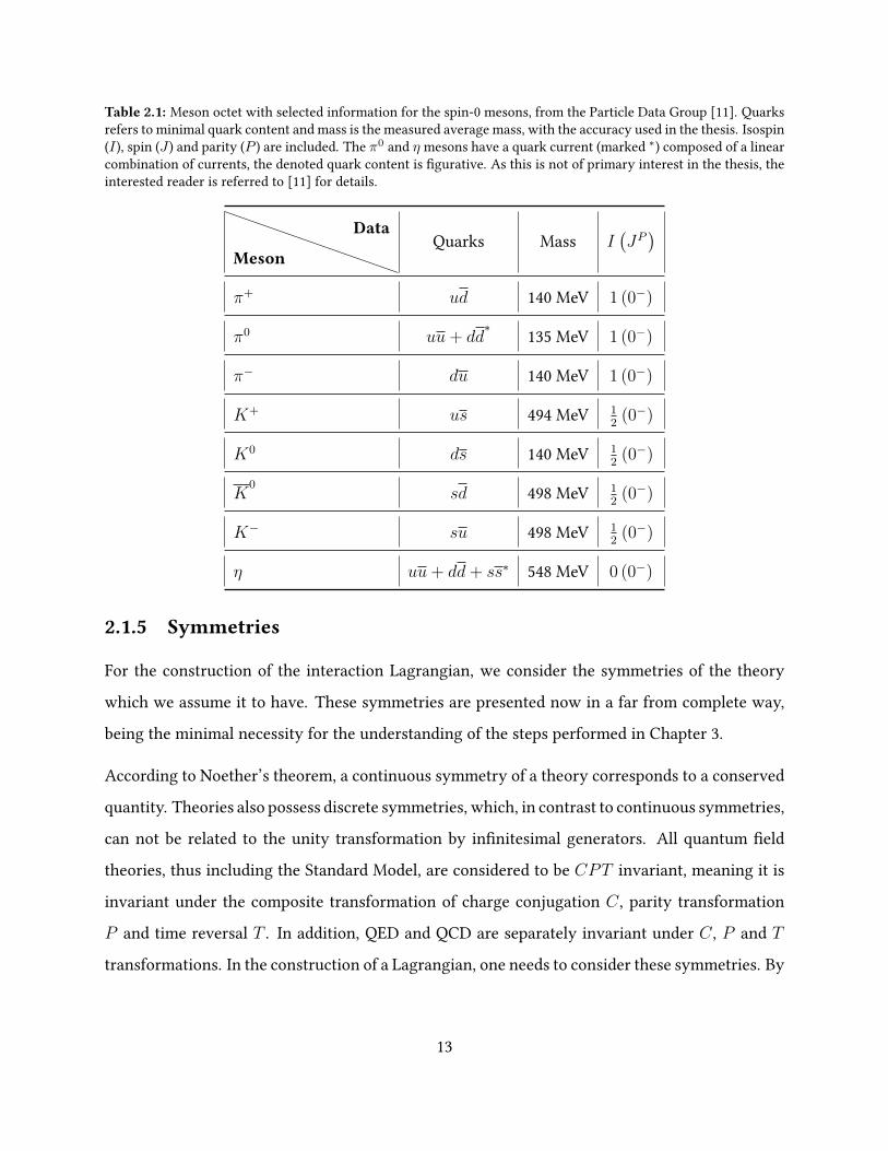
Table 2.1: Meson octet with selected information for the spin-0 mesons, from the Particle Data Group [11]. Quarksrefers to minimal quark content and mass is the measured average mass, with the accuracy used in the thesis. Isospin(I), spin (J ) and parity (P ) are included. The π0 and η mesons have a quark current (marked ∗) composed of a linearcombination of currents, the denoted quark content is gurative. As this is not of primary interest in the thesis, theinterested reader is referred to [11] for details.
Meson
DataQuarks Mass I
(JP)
π+ ud 140 MeV 1 (0−)
π0 uu+ dd∗ 135 MeV 1 (0−)
π− du 140 MeV 1 (0−)
K+ us 494 MeV 12
(0−)
K0 ds 140 MeV 12
(0−)
K0
sd 498 MeV 12
(0−)
K− su 498 MeV 12
(0−)
η uu+ dd+ ss∗ 548 MeV 0 (0−)
2.1.5 Symmetries
For the construction of the interaction Lagrangian, we consider the symmetries of the theory
which we assume it to have. These symmetries are presented now in a far from complete way,
being the minimal necessity for the understanding of the steps performed in Chapter 3.
According to Noether’s theorem, a continuous symmetry of a theory corresponds to a conserved
quantity. Theories also possess discrete symmetries, which, in contrast to continuous symmetries,
can not be related to the unity transformation by innitesimal generators. All quantum eld
theories, thus including the Standard Model, are considered to be CPT invariant, meaning it is
invariant under the composite transformation of charge conjugation C , parity transformation
P and time reversal T . In addition, QED and QCD are separately invariant under C , P and T
transformations. In the construction of a Lagrangian, one needs to consider these symmetries. By
13
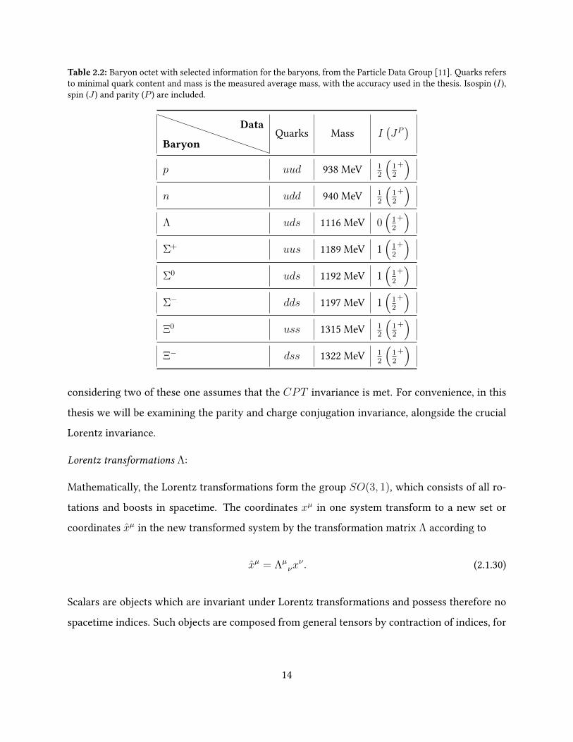
Table 2.2: Baryon octet with selected information for the baryons, from the Particle Data Group [11]. Quarks refersto minimal quark content and mass is the measured average mass, with the accuracy used in the thesis. Isospin (I),spin (J ) and parity (P ) are included.
Baryon
DataQuarks Mass I
(JP)
p uud 938 MeV 12
(12
+)
n udd 940 MeV 12
(12
+)
Λ uds 1116 MeV 0(
12
+)
Σ+ uus 1189 MeV 1(
12
+)
Σ0 uds 1192 MeV 1(
12
+)
Σ− dds 1197 MeV 1(
12
+)
Ξ0 uss 1315 MeV 12
(12
+)
Ξ− dss 1322 MeV 12
(12
+)
considering two of these one assumes that the CPT invariance is met. For convenience, in this
thesis we will be examining the parity and charge conjugation invariance, alongside the crucial
Lorentz invariance.
Lorentz transformations Λ:
Mathematically, the Lorentz transformations form the group SO(3, 1), which consists of all ro-
tations and boosts in spacetime. The coordinates xµ in one system transform to a new set or
coordinates xµ in the new transformed system by the transformation matrix Λ according to
xµ = Λµνx
ν . (2.1.30)
Scalars are objects which are invariant under Lorentz transformations and possess therefore no
spacetime indices. Such objects are composed from general tensors by contraction of indices, for
14
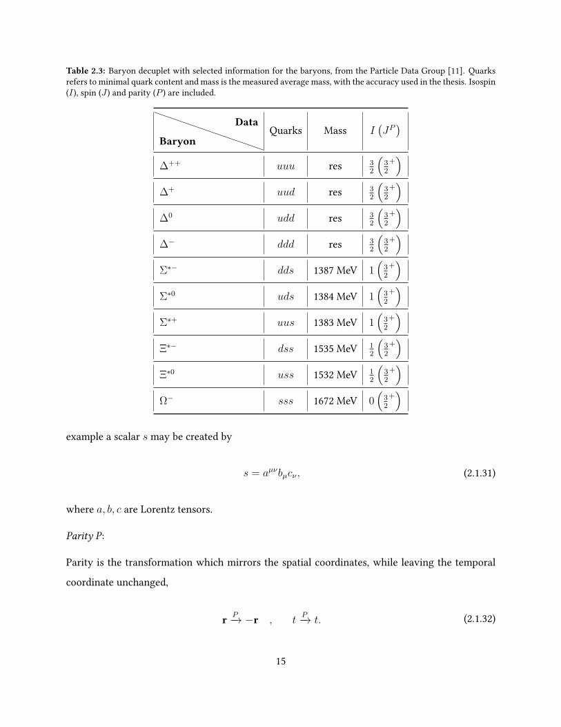
Table 2.3: Baryon decuplet with selected information for the baryons, from the Particle Data Group [11]. Quarksrefers to minimal quark content and mass is the measured average mass, with the accuracy used in the thesis. Isospin(I), spin (J ) and parity (P ) are included.
Baryon
DataQuarks Mass I
(JP)
∆++ uuu res 32
(32
+)
∆+ uud res 32
(32
+)
∆0 udd res 32
(32
+)
∆− ddd res 32
(32
+)
Σ∗− dds 1387 MeV 1(
32
+)
Σ∗0 uds 1384 MeV 1(
32
+)
Σ∗+ uus 1383 MeV 1(
32
+)
Ξ∗− dss 1535 MeV 12
(32
+)
Ξ∗0 uss 1532 MeV 12
(32
+)
Ω− sss 1672 MeV 0(
32
+)
example a scalar s may be created by
s = aµνbµcν , (2.1.31)
where a, b, c are Lorentz tensors.
Parity P :
Parity is the transformation which mirrors the spatial coordinates, while leaving the temporal
coordinate unchanged,
r P−→ −r , tP−→ t. (2.1.32)
15
In general a four-vector aµ transforms as
aµP−→ Πµ
νaν , (2.1.33)
where Πµν is the parity matrix dened as
(Πµν) =
1 0 0 00 −1 0 00 0 −1 00 0 0 −1
. (2.1.34)
Scalar particle elds Φ are eigenstates of parity with eigenvalue p which must square to unity, as
acting parity twice on a eld must by denition recover the original eld,
(P−1)2Φ(x)P 2 = p2Φ(x)!
= Φ(x). (2.1.35)
However, in the case of fermionic elds, there is a simple caveat: single elds are not observ-
ables, but rather a pair of elds is observable, which transforms back to itself under two parity
transformations. This leads to the parity transformation of Dirac elds being
P−1Ψ(x)P = iγ0Ψ(Πx),
P−1Ψ(x)P = −iΨ(Πx)γ0,(2.1.36)
which together imply that the mass term ΨΨ in the Dirac Lagrangian indeed is a scalar.
Charge conjugation C:
Under charge conjugation, all charges (corresponding to any conserved current) change to their
opposite, which means particles are transformed into their antiparticles. Dirac elds transform in
a specic way, which ensures that the Dirac Lagrangian stays invariant under charge conjugation,
C−1Ψ(x)C = C ΨT
(x),
C−1Ψ(x)C = ΨT (x)C .(2.1.37)
16
We note that the spacetime argument is not transformed. The charge conjugation matrix C is in
Weyl representation given by
C =
0 −1 0 01 0 0 00 0 0 10 0 −1 0
. (2.1.38)
The photon eld transforms as
C−1Aµ(x)C = −Aµ(x). (2.1.39)
It is straightforward in the given representation to derive the following properties between the
gamma matrices and C :
C −1γµC = −(γµ)T ,
C −1γ5C = γ5,
C T =C −1 = −C .
(2.1.40)
Having introduced the two discrete symmetries and Lorentz transformations, we can now handle
the symmetry invariances we will assume the theory of the interacting hyperons to have. We
now move on to present the eective eld theory framework and specically chiral perturbation
theory, which is not explicitly used in this thesis, but being the method used to obtain the results
for the scattering amplitudes. The results obtained with this method is then used in the dispersive
approach in this thesis.
2.2 Eective eld theories
The model of description in physics depends on which scale of examination we are interested in.
In the case of QCD, one might consider to treat quarks as the relevant degrees of freedom (which
up to today we consider to be fundamental particles), in which case the energies of examination
must be high enough for the coupling to be treated perturbatively. At low energies, however, the
17
quarks can no longer be treated as the relevant degrees of freedom. In this region, we consider
instead the hadrons as fundamental degrees of freedom. The theory is now an eective eld
theory, as it includes those scales at which we can observe, rather than (what we think is) the
fundamental building blocks. We will here briey introduce chiral perturbation theory [12, 13],
which is one of the most used eective eld theories for low-energy strong interaction.
2.2.1 Chiral perturbation theory
In the theory of the strong interaction of the standard model, we describe the interactions between
quarks and gluons. Due to the running of the strong coupling constant, we can apply perturbation
theory in the coupling constant only at high energies, above ΛQCD ≈ (100− 300) MeV [11]. At
lower energies, which we will refer to here as low-energy regime, we can no longer perform
this perturbative expansion in the coupling. Due to connement, free quarks are never observed,
only in the composite states as hadrons. In the low-energy regime, where the coupling is very
strong, the free-particle behavior of the quarks is suppressed and we consider the hadrons as the
pointlike objects in the theory.
For low energies, instead of performing perturbative expansion in the coupling constant, we
may expand in the momentum space. In real space this translates into expanding in powers
of derivatives. This approach is named eective eld theories. The eective eld theory we
encounter here is chiral perturbation theory. In this approach, the chiral symmetry of QCD, the
independent transformation of right- and left-handed spinors, is respected. The only degrees of
freedom which can be excited are the lightest hadrons — these are the eight Goldstone bosons:
π0, π±, K±, K0, K0, η, which are collected in a U ∈ SU(3) matrix,
U(x) = eiφ(x), (2.2.1)
18
with the Goldstone boson elds in the matrix φ(x) according to
φ(x) =
π0(x) + 1√
3η(x)
√2π+(x)
√2K+(x)
√2π−(x) −π0(x) + 1√
3η(x)
√2K0(x)
√2K−(x)
√2K
0(x) − 2√
3η(x)
. (2.2.2)
Expanding U(x) in the chiral Lagrangian gives dierent powers of the Goldstone boson elds.
Being the lightest ones, π± and π0 are the ones excited at the lowest energies. In the same manner,
one includes octet and decuplet baryons in the chiral Lagrangian and in that manner, by expand-
ing in powers of momenta, obtains the leading-order contributions of all hadronic interactions,
then next-to-leading order, then next-to-next-to-leading order, and continuing to all orders.
In this thesis we will initially only consider the two hyperons Σ∗ and Λ interacting electromag-
netically, not including any of the Goldstone bosons. For the second part of the thesis, which
comprises the dispersive analysis, we need the amplitudes including also the octet baryon Σ. The
amplitudes are calculated and presented by Junker [3, 14] and will be used as input to the present
work.
2.2.2 Vertex functions and form factors
In hadronic physics, the internal structures of the hadrons are examined. At low energies, the
building blocks of hadrons are very strongly interacting and the composite objects are considered
as pointlike. To resolve the internal structure, form factors are used. One considers the scattering
of hadrons with other particles to obtain the information about the internal structure.
The crucial experiment leading to the discovery of quarks was the famous deep-inelastic scat-
tering performed at the Stanford Linear Accelerator Center (SLAC) [15], where the scattering of
protons and electrons was examined. The experiment, performed at very high energies resolved
almost free quarks and so the quark structure was more clearly visible.
At low energies, the prominent probing is through the electromagnetic interaction. As quarks
are charged, any hadron interacts electromagnetically, even though the composite hadron might
19
e− e−
B B′
γ
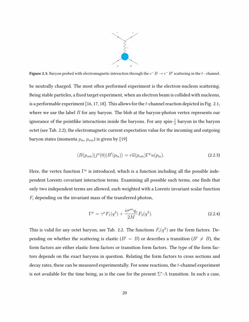
Figure 2.1: Baryon probed with electromagnetic interaction through the e−B → e−B′ scattering in the t−channel.
be neutrally charged. The most often performed experiment is the electron-nucleon scattering.
Being stable particles, a xed target experiment, when an electron beam is collided with nucleons,
is a performable experiment [16, 17, 18]. This allows for the t-channel reaction depicted in Fig. 2.1,
where we use the label B for any baryon. The blob at the baryon-photon vertex represents our
ignorance of the pointlike interactions inside the baryons. For any spin-12
baryon in the baryon
octet (see Tab. 2.2), the electromagnetic current expectation value for the incoming and outgoing
baryon states (momenta pin, pout) is given by [19]
〈B(pout)|jµ(0)|B′(pin)〉 = eu(pout)Γµu(pin). (2.2.3)
Here, the vertex function Γµ is introduced, which is a function including all the possible inde-
pendent Lorentz covariant interaction terms. Examining all possible such terms, one nds that
only two independent terms are allowed, each weighted with a Lorentz invariant scalar function
Fi depending on the invariant mass of the transferred photon,
Γµ = γµF1(q2) +iσµνqν
2MF2(q2). (2.2.4)
This is valid for any octet baryon, see Tab. 2.2. The functions Fi(q2) are the form factors. De-
pending on whether the scattering is elastic (B′ = B) or describes a transition (B′ 6= B), the
form factors are either elastic form factors or transition form factors. The type of the form fac-
tors depends on the exact baryons in question. Relating the form factors to cross sections and
decay rates, these can be measured experimentally. For some reactions, the t-channel experiment
is not available for the time being, as is the case for the present Σ∗-Λ transition. In such a case,
20
form factors in one region may still be related to other regions in a theoretical approach with aid
of dispersion relations. This is the topic for Chapters 5 and 6 of this thesis.
Some denition of terminology for the dierent energy regions must be made. For an electromag-
netic probing in a one-photon approximation, the photon carries the transferred momentum q2
in the interaction. Depending on the kinematical reaction being considered, q2 is either positive,
negative or zero. For a real massless photon, the invariant mass vanishes, q2 = 0. If the invariant
mass satises q2 < 0, the region is called spacelike. If the invariant mass satises q2 > 0, the
region is called timelike.
2.3 Scattering theory
Particle properties are most easily examined through their interactions with other particles. This
leads to the concept of scattering, the interaction of several particles. On the one hand, we have
the case of two particles colliding, creating a set of particles (which can also be the same as the
initial set). These reactions are scattering reactions and experimentally one measures the cross
section, related to the probability of the reaction occurring. On the other hand, one may consider
the transformation of a single particle into a new set of particles, which is referred to as a decay
reaction. The measured quantity in this case is a decay rate, once again the probability of the
given decay to occur.
Being probabilities, both of these measured quantities need the quantum mechanical amplitude
of the two states before and after the reaction. For this, one introduces the S-operator, which
gives the time evolution from the initial state to the nal. Consider the reaction occurring at
t = 0, and let the initial state and nal state be Ψi(ti) and Ψf (tf ) respectively, at times ti < 0
and tf > 0, which are related by the time evolution operator of the interacting Hamiltonian,
|Ψf (tf )〉 = U int(tf , ti) |Ψi(ti)〉 . (2.3.1)
Dividing the time interval at the point t = 0, we relate the in and out states at the same time
21
related by the free Hamiltonian,
UF(tf , 0) |Ψf (0)〉 = |Ψf (tf )〉 ,
UF(ti, 0) |Ψi(0)〉 = |Ψi(ti)〉 ,(2.3.2)
which allows us to relate
|Ψf (0)〉 = UF(0, tf )Uint(tf , ti)U
F(ti, 0)︸ ︷︷ ︸=:U(tf ,ti)
|Ψi(0)〉 . (2.3.3)
The S-operator is dened in the limit ti → −∞, tf →∞,
S := limti→−∞tf→∞
U(tf , ti). (2.3.4)
In a eld theory with the interaction Lagrangian Lint, the S-operator is given by
S = ei∫
d4xLint . (2.3.5)
The case of no reaction of occurring is implemented in the S-operator by dening S =: 1+ iT ,
with T carrying all the interaction information. The invariant matrix element M is dened by
〈Ψf (tf )|iT |Ψi(ti)〉 =: (2π)4δ(4)(∑
pin −∑
pout
)iM , (2.3.6)
where the sum is over all the incoming and outgoing momenta, respectively.
We now present the dierential cross section for a 2 → n scattering. Letting the incoming
momenta of the two particles be p1 and p2, and the outgoing particle momenta be q1, ..., qn, the
dierential cross section is given by
dσ =1
4|p1|√s|M |2(2π)4δ(4)
(p1 + p2 −
n∑i=1
qi
)n∏i=1
dqi, (2.3.7)
22
where p1 is the three-momentum of the incoming momenta in the center of momentum (CM)
frame. We use the tilde abbreviation introduced in (2.1.8).
From this, the 2 → 2 solid angle dierential cross section can be derived by performing the
integration. In the CM frame this is
(dσdΩ
)CM
=1
64π2s|M |2 |p1|
|q1|, (2.3.8)
with the outgoing three-momentum q1. This expression will be used for the calculation of the
dierential cross section for the reaction e+e− → Σ∗Λ in Chapter 4.
One similarly denes the dierential decay rate for a 1 → n decay, in the rest frame of the
decaying particle with mass M and momentum p, into particles with momenta q1, ..., qn as
dΓ =1
2M|M |2(2π)4δ(4)
(p−
n∑i=1
qi
)n∏i=1
dqi. (2.3.9)
The cases we will need are the n = 2 decay for the real-photon decay Σ∗ → Λγ, and the n = 3
case for the Dalitz decay Σ∗ → Λe+e−. The decay rates for these reactions are considered in
Chapter 4.
2.4 The Σ∗-Λ transition
From the Particle Data Group [11], we obtain the full measured decay width of the neutrally
charged unstable Σ∗0(1385) resonance,
Γ = 36± 5 MeV. (2.4.1)
23
The largest measured branching ratios are:
Σ∗0 → Λπ , Γi/Γ ≈ 87.0%,
Σ∗0 → Σπ , Γi/Γ ≈ 11.7%,
Σ∗0 → Λγ , Γi/Γ ≈ 1.25%.
(2.4.2)
We will explicitly calculate the decay rate in terms of the form factors for the last decay channel
in Chapter 4.
The study of the decay of such particles with a structure dierent to the nucleons might yield
insight into the fundamental building blocks of Nature. In a previous work by Granados et al. [2],
the electromagnetic transition form factors at low energies for the ground-state Σ0-Λ transition
have been studied. However, for the case of the Σ∗0-Λ transition, the larger mass of Σ∗0 leads
to an anomalous threshold, which changes the analytic structure of the form factors. The Dalitz
decay Σ∗0 → Λe+e− which can presently be performed, is probed in the kinematical region
4m2e < q2 < (mΣ∗ −mΛ)2 of the invariant mass q2 of the transferred momentum. This means
that we cover a larger energy interval than in the Σ0-Λ case, which gives more space to explore
the q2 dependence of the form factors. For convenience, we omit the explicit charge superscript
and mass specication for the particles, understanding that we work only with the neutral, rst
excitation of the Σ particle, the Σ∗ particle, and the Λ particle.
With this we conclude the background theory to the thesis. In the coming chapter we present the
interaction Lagrangian, introduce the form factors and present a step by step construction of the
vertex function for this spin-32
to spin-12
(decuplet-octet baryon) transition, in terms of the form
factors.
24
Chapter 3
Feynman rules
In the spirit of the octet baryon electromagnetic current and vertex function given in (2.2.3),
we will here dene the vertex function for the decuplet-octet baryon transition. Our starting
denition is an incoming Σ∗Λ state, and an outgoing photon,
〈0|jµ(0)|Σ∗(pΣ∗)Λ(pΛ)〉 =: evΛ(pΛ)ΓµνuΣ∗
ν (pΣ∗), (3.0.1)
which is needed for the one-photon approximation with which we calculate the decay rate and
cross sections later. We suppress the spin arguments of the spinor and vector-spinor.
With charge conjugation and crossing symmetry, the vertex function can be related to any other
reaction (with other incoming and outgoing states) of the Σ∗Λγ interaction.
The two Lorentz indices in Γµν arise from the electromagnetic current and the Lorentz index for
the vector-spinor of the spin-32
Σ∗ particle. In this chapter we will construct step by step the form
of the vertex function from this denition. The vertex function is found to be parametrized by
three independent functions, which will be the three electromagnetic transition form factors. We
follow the construction of the interaction Lagrangian based on parity, charge conjugation and
Lorentz invariance (and the usual gauge invariance). Based on this, we formulate the Feynman
rules for the theory.
25
3.1 Parity transformation of vertex function
The parity transformation of the spin-12
spinors is covered in textbooks on quantum eld the-
ory [4, 5, 6]. The transformation of the spin-32
vector-spinor is not trivial and the derivation is
presented here [7]. We assume a parity conserving vacuum and particle theory, meaning a P
conserving electromagnetic and strong interaction.
Insert twice the identity, 1 = PP−1 = PP † in the matrix element in the denition of the vertex
function (3.0.1),
〈0|P †P︸︷︷︸=1
jµ(0)P−1P︸ ︷︷ ︸=1
|Σ∗(pΣ∗)Λ(pΛ)〉 = evΛ(pΛ)ΓµνuΣ∗
ν (pΣ∗). (3.1.1)
The vacuum state, being an eigenstate of the full Hamiltonian, is assumed to be parity invariant,
P |0〉 = |0〉 ↔ 〈0|P † = 〈0| . (3.1.2)
The Σ∗ has positive parity, JP = 32
+, and the Λ, JP = 12
+, also has positive parity, while the
corresponding antiparticles have opposite parity. The two-particle state transforms then as
P |Σ∗(pΣ∗)Λ(pΛ)〉 = − |Σ∗(ΠpΣ∗)Λ(ΠpΛ)〉 , (3.1.3)
and with the usual transformation of a Lorentz vector for the current,
Pjµ(0)P−1 = Πµνjν(0), (3.1.4)
where the argument is unchanged under parity transformation.
With these we can rewrite the left-hand side of (3.1.1),
−Πµν 〈0|jν(0)|Σ∗(ΠpΣ∗)Λ(ΠpΛ)〉︸ ︷︷ ︸
use (3.0.1)
= evΛ(pΛ)ΓµνuΣ∗
ν (pΣ∗). (3.1.5)
26
For the depicted part of the left-hand side, we use the denition of the vertex function (3.0.1)
evaluated at negative momenta, meaning that the four-momentum p argument becomes Πp,
〈0|jν(0)|Σ∗ (ΠpΣ∗) Λ (Πpλ)〉 = evΛ (ΠpΛ) ΓνβuΣ∗
β (ΠpΣ∗) , (3.1.6)
where Γµν is the vertex function evaluated at negative momenta. Inserting this back into (3.1.5),
−ΠµνvΛ (ΠpΛ) ΓνβuΣ∗
β (ΠpΣ∗) = vΛ(pΛ)ΓµνuΣ∗
ν (pΣ∗). (3.1.7)
The ipped momentum relations for spin-12
spinors are [4]
u(Πp) = γ0u(p),
v(Πp) = −γ0v(p),
u(Πp) = u(p)γ0,
v(Πp) = −v(p)γ0.
(3.1.8)
Given a general three-momentum p, we can always perform a rotation to a frame in which the
momentum is along the z-axis. We therefore consider the momentum ip in this frame, with
momentum pµ = (E, 0, 0, pz), with E =√p2z +m2 and m being the mass of the particle. Using
the denition of vector-spinors (2.1.24), we now see how the corresponding momentum-ipped
relations are. In the frame of p = pz z the polarization vector is expressed as
εµ(p, s = ±1) =±1√
2(0, 1,∓i, 0),
εµ(p, s = 0) =1
m(pz, 0, 0, E).
(3.1.9)
The change under parity transformation is immediate,εµ(p, s = ±1) = ±1√2(0, 1,∓i, 0)
εµ(p, s = 0) = 1m
(pz, 0, 0, E)
P−→
εµ(Πp, s = ±1) = ±1√2(0, 1,∓i, 0)
εµ(Πp, s = 0) = 1m
(−pz, 0, 0, E),(3.1.10)
27
which is expressed as
εµ(p, s) = −Πµνεν(Πp, s) ↔ εν (Πp, s) = −Π ν
µ εµ(p, s). (3.1.11)
We can then perform the momentum ip for the vector-spinor using (3.1.8) and (3.1.11),
uµ(Πp, s) =∑s′,s′′
Cs,s′,s′′
(1,
1
2
)u(Πp, s′)εµ(Πp, s′′) =
= −Π µν γ0
∑s′,s′′
Cs,s′,s′′
(1,
1
2
)u(p, s′)εν(p, s′′) = −Π µ
ν γ0uν(p, s).
(3.1.12)
Inserting now the momentum-ip relations for the vector-spinor (3.1.12) and the momentum ip
of the spin-12
spinors (3.1.8) into (3.1.7) gives
−ΠµνΠ
αβvΛ (pΛ) γ0Γνβγ0u
Σ∗
α (pΣ∗) = vΛ(pΛ)ΓµνuΣ∗
ν (pΣ∗). (3.1.13)
This nally gives the condition for the vertex function
−ΠµνΠ
αβγ0Γνβγ0
!= Γµα. (3.1.14)
This requirement ensures that the hyperon states transform accordingly under parity. Therefore
we shall now refer to this condition (3.1.14) as parity transformation of the vertex function.
3.2 Vertex function and form factors
In this section we follow the construction of the vertex function Γµν in the denition (3.0.1) by
considering the symmetries of the theory. Following this denition, we consider an incoming Σ∗
with momentum pΣ∗ and an incoming Λ with momentum pΛ and an outgoing (virtual) photon
with momentum q = pΣ∗+pΛ. The two momenta pΣ∗ and pΛ are the only independent parameters
in the vertex. Equivalently, we may express the two independent parameters by the sum q and
by pΣ∗ . Thus, any Lorentz invariant function will depend only on the invariant combinations of
28
these: q2, p2Σ∗ or q · pΣ∗ , but since p2
Σ∗ = m2Σ∗ , this is just a constant in our theory. Further, we
can rewrite
pΣ∗ · q =1
2
(p2
Σ∗ + q2 − (q − pΣ∗)2)
=1
2
(p2
Σ∗ + q2 − p2Λ
), (3.2.1)
which is completely determined by q2, as also p2Λ = m2
Λ is not a parameter. We are then left with
only one independent parameter of the vertex, and we shall use q2.
We distinguish between objects with spinor structure and those without. A general bilinear of
the form ΨBΨ, with B being a spinor matrix, can transform under Lorentz transformations in
dierent ways. We may expand B in a basis where each term transforms uniquely. A standard
choice of such basis is
1, γµ, γ5, γ5γµ, σµν, (3.2.2)
where µ = 0, 1, 2, 3 are Lorentz indices and so in total we have 16 objects in this basis. The
denition of the gamma tensor (2.1.5) may be rewritten in a convenient form
σµν =i
2(γµ, γν − 2γνγµ) =
i
2(2gµν − 2γνγµ) = i(gµν − γνγµ). (3.2.3)
The identity (3.2.3) can be used to change the gamma tensor to two gamma matrices (and the
identity spinor structure 1), resulting in a new basis which we will use in the construction,
1, γµ, γ5, γ5γµ, γµγν. (3.2.4)
The Lorentz covariant objects without explicit spinor structure are
qµ, pµΣ∗ , gµν , εµναβ. (3.2.5)
Working with the Levi-Civita tensor can however be tedious. We note that it may be rewritten
29
as
εµναβ = εµναβγ5γ5 = − i
4!εµναβεστρλγσγτγργλγ5 =
=i
4!
∣∣∣∣∣∣∣∣∣∣∣∣
gµσ gµτ gµρ gµλ
gνσ gντ gνρ gνλ
gασ gατ gαρ gαλ
gβσ gβτ gβρ gβλ
∣∣∣∣∣∣∣∣∣∣∣∣γσγτγργλγ5,
(3.2.6)
which essentially rewrites the Levi-Civita tensor in terms of four gamma matrices and a γ5. In
this spirit, we will, instead of using the basis (3.2.4), use arbitrary number of gamma matrices and
one γ5, and omit the usage of the Levi-Civita tensor.
We set an upper boundary to the number of gamma tensors allowed this way. The Lorentz objects
without spin structure we denote generally with xwith corresponding number of indices. Objects
with three gamma matrices such as
γµγνγαxα, (3.2.7)
may be terms with four-momenta only, in which case a four-momentum (p) is contracted with a
gamma matrix. In those cases, we can use the Dirac equation (2.1.7) to eliminate the γµpµ = /p
to m, in which case the term becomes redundant to those without the /p structure. Similarly, the
non-spinor structure in the terms on the form
γµγαγβxµαβ, (3.2.8)
in the same way can be several four-momenta or a metric tensor and a four-momenta. A met-
ric tensor simply raises the index of a gamma matrix, which then gets contracted with another
gamma matrix, which reduces the form. Lastly, a similar argument follows for the terms on the
form
γλγαγβxµναβλ. (3.2.9)
30
A similar argumentation can be performed for higher number of gamma matrices. At the end,
we are reduced to a highest number of two gamma matrices.
The most general form of the vertex function will be a covariant expression which satises
Lorentz invariance. Each term in the expression will consist of a Lorentz invariant coecient,
a spinor structure (of up to two gamma matrices with or without a γ5) and a covariant object
without spinor structure. As stated earlier, the only independent Lorentz invariant quantity in
the reaction is q2, thus all Lorentz invariant coecients (Ak, Bk...) in the terms are allowed to
depend on this quantity. We sum all possible such terms,
Γµν =∑k
(Ak(q2)1aµνk + Ak(q
2)γ5aµνk +
+Bk(q2)γµbνk + Bk(q
2)γν bµk + Bk(q2)γαb
µναk +
+ +Ck(q2)γµγ5c
νk + Ck(q
2)γνγ5cµk + Ck(q
2)γαγ5cµναk +
+R(q2)γµγν+
+Dk(q2)γµγαd
ανk + Dk(q
2)γνγαdαµk + Dk(q
2)γαγβdαβµνk +
+ S(q2)γµγνγ5+
+ Ek(q2)γµγαγ5e
ανk + Ek(q
2)γνγαγ5eαµk + Ek(q
2)γαγβγ5eαβµνk
(3.2.10)
Any other object in the Lorentz covariant form can also include contractions, for example a term
with two Lorentz indices such as gµν can equally well be accompanied by arbitrary number of
contractions, building Lorentz invariant structures,
gµνpαΣ∗qαεστλγqσ(pΣ∗)τ (pΣ∗)λ(pΣ∗)γ, (3.2.11)
however we note that we can implement all such contracted additions in the Lorentz invariant
coecients accompanying each term.
The non-spinor objects with three Lorentz indices can either be three four-momenta, or a four-
momentum and a metric. Similarly, four-index objects can either be four four-momenta, two
metrics or a metric and two four-momenta. Two-index objects are either two momenta or a
31
metric. When a four-momentum is contracted with a gamma matrix however, we can use the
Dirac equation to reduce it. As an example, let us examine the term
gµνqαpβΣ∗ . (3.2.12)
Such a term when inserted in the matrix element (3.0.1) will give
vΛ(pΛ)[γαγβgµνqαpβΣ∗ ]u
Σ∗
ν (pΣ∗) = vΛ(pΛ)[gµν(/pΣ∗+ /pΛ
)/pΣ∗]uΣ∗
ν (pΣ∗) =
= vΛ(pΛ)[gµν(mΛ −mΣ∗)(−mΣ∗)]uΣ∗
ν (pΣ∗)
∝ vΛ(pΛ)[gµν ]uΣ∗
ν (pΣ∗),
(3.2.13)
using (2.1.7) to eliminate the slashed momenta. This is thus redundant to terms without any
gamma matrices. At the end, the possible Lorentz objects are (including the spinor object, ex-
cluding the explicit Lorentz-invariant coecients)
gµν , pµΣ∗pνσ∗ , p
µΣ∗q
νσ∗ , q
µΣ∗p
νσ∗ , q
µΣ∗q
νσ∗ ,
gµνγ5, pµΣ∗p
νσ∗γ5, p
µΣ∗q
νσ∗γ5, q
µΣ∗p
νσ∗γ5, q
µΣ∗q
νσ∗γ5,
γµpνΣ∗ , γµqν , γνpµΣ∗ , γ
νpµΣ∗ , γαgµαpνΣ∗ , γαg
µαqν , γαgναpµΣ∗ , γαg
ναqµ,
γµpνΣ∗γ5, γµqνγ5, γ
νpµΣ∗γ5, γνpµΣ∗γ5, γαg
µαqνγ5, γαgναpµΣ∗γ5, γαg
ναqµγ5,
γµγν , γµγνγ5,
γµγαgνα, γνγαg
µα, γαγβgαβpµΣ∗p
νΣ∗ , γαγβg
αβpµΣ∗qν , γαγβg
αβqµpνΣ∗ , γαγβgαβqµqν ,
γµγαγ5gνα, γνγαγ5g
µα, γαγβγ5gαβpµΣ∗p
νΣ∗ , γαγβγ5g
αβpµΣ∗qν , γαγβγ5g
αβqµpνΣ∗ , γαγβγ5gαβqµqν .
(3.2.14)
For the three- and four-index structures, we note that in the construction (3.2.10), all such terms
come with contracting one index with one or two gamma matrices. All terms where the con-
tracted index is one of a momentum, the Dirac equation (2.1.7) can be used to eliminate it. In a
similar manner all such possibilities can be disposed of.
Next, we recall the Rarita-Schwinger constraint (2.1.27) on the spin-32
vector-spinor elds, and the
32
orthogonality relation (2.1.29). The ν index in the vertex function is contracted with the vector-
spinor eld. Thus, when this free index is carried by the Σ∗ four-momentum, the term vanishes
(orthogonality). Similarly, if the free index is carried by a gamma matrix, the term vanishes
(Rarita-Schwinger constraint).
At the end, the possibilities which are left after using the Dirac equation, the orthogonality and
the Rarita-Schwinger constraint on the vector-spinor elds, are the terms
Γµν = A1(q2)gµν + A2(q2)qµqν + A3(q2)pµΣ∗qν +B1(q2)γµqν+
+ A1(q2)γ5gµν + A2(q2)γ5q
µqν + A3(q2)γ5pµΣ∗q
ν + C1(q2)γµγ5qν .
(3.2.15)
We shall now use the parity transformation condition (3.1.14) for the vertex function. The mo-
mentum ip (being terms in Γµν) of the non-spinor structures in the ansatz (3.2.15) are
gµνP−→ gµν , qµqν
P−→ ΠµσΠν
τqσqτ ,
pµΣ∗qν P−→ Πµ
σΠντ (pΣ∗)
σqτ , γµqνP−→ Πν
σγµqσ.
(3.2.16)
Using the terms without a gamma matrix in (3.1.14) trivially,
− ΠµνΠ
αβγ0(gνβ)γ0 = −gµα 6= gµα,
− ΠµνΠ
αβγ0(Πν
σΠβτqσqτ )γ0 = −qµqα 6= qµqα,
− ΠµνΠ
αβγ0(Πµ
σΠντ (pΣ∗)
σqτ )γ0 = −pµΣ∗qα 6= pµΣ∗qα,
(3.2.17)
meaning that the rst three terms violate the parity transformation. The fourth term is slightly
non-trivial,
−ΠµνΠ
αβγ0(Πβ
σγνqσ)γ0 = −Πµ
νqαγ0γ
νγ0, (3.2.18)
where we will use the anticommutation relation γµ, γν = 2gµν , to obtain γ0γiγ0 = −γi and
33
γ0γ0γ0 = γ0, which can be fused in γ0γµγ0 = Πµ
νγν , giving
−ΠµνΠ
αβγ0(Πβ
σγνqσ)γ0 = −Πµ
νqαΠν
βγβ = −γµqα 6= γµqα. (3.2.19)
The terms with γ5 include an additional sign change due to the anti-commutation γ5, γµ = 0,
− ΠµνΠ
αβγ0(γ5g
νβ)γ0 = gµα,
− ΠµνΠ
αβγ0(γ5Πν
σΠβτqσqτ )γ0 = qµqα,
− ΠµνΠ
αβγ0(γ5Πν
σΠβτ (pΣ∗)
σqτ )γ0 = pµΣ∗qα,
− ΠµνΠ
αβγ0(Πβ
σγ5γνqσ)γ0 = γ5γ
µqα,
(3.2.20)
all satisfying the parity condition (3.1.14). Finally, the terms left in (3.2.15) which also satisfy the
parity transformation, are
Γµν = A1(q2)γ5gµν + A2(q2)γ5q
µqν + A3(q2)γ5pµΣ∗q
ν + C1(q2)γµγ5qν . (3.2.21)
Next we will use current conservation, ∂µjµ(x) = 0. This equation holds as an operator identity,
for any states. To use this on the current evaluated at x = 0, we need to perform a translation in
spacetime of the correlator with the translation operator T (x− x0) = e−iP (x−x0),
〈0|jµ(x)|Σ∗(pΣ∗)Λ(pΛ)〉 = 〈0|eiPxjµ(0)e−iPx|Σ∗(pΣ∗)Λ(pΛ)〉 =
= e−iqx 〈0|jµ(0)|Σ∗(pΣ∗)Λ(pΛ)〉 ,(3.2.22)
with q = pΣ∗ + pΛ being the total momentum of the two-hadron state.
Applying now the partial derivative ∂µ to the right- and left-hand side of (3.2.22) gives
−iqµe−iqx 〈0|jµ(0)|Σ∗(pΣ∗)Λ(pΛ)〉 = 0, (3.2.23)
which is only valid as a correlator equation. By contracting with the total momentum qµ of the
34
two-hadron state in the denition of the vertex function (3.0.1)
qµ 〈0|jµ(0)|Σ∗(pΣ∗)Λ(pΛ)〉 = evΛ(pΛ)qµΓµνuΣ∗
ν (pΣ∗)!
= 0. (3.2.24)
Using the form (3.2.21) for the vertex function, contracting with qµ gives
vΛ [A1(q2) + A2(q2)q2 + A3(q2)(pΣ∗ · q) + C1(q2)/q]γ5︸ ︷︷ ︸!=0
qνuΣ∗
ν = 0. (3.2.25)
With this, we eliminate one of the Lorentz invariant functions,
A1(q2) = −A2(q2)q2 − A3(q2)(pΣ∗ · q)− C1(q2)/q, (3.2.26)
and the vertex function becomes (moving the γ5 to the right by convention)
Γµν = −C1(q2)(γµqν − /qgµν)γ5+
+ A3(q2)(pµΣ∗qν − (pΣ∗ · q)gµν)γ5+
+ A2(q2)(qµqν − q2gµν)γ5.
(3.2.27)
We now dene the three electromagnetic transition form factors Fi(q2) ∈ C by
F1(q2) :=C1(q2)
mΣ∗,
F2(q2) := A3(q2),
F3(q2) := A2(q2),
(3.2.28)
where we have introduced the mass mΣ∗ for the three form factors to have the same dimension.
35
Making these denitions, the vertex function (3.2.27) in terms of the form factors becomes
Γµν = −mΣ∗F1(q2)(γµqν − /qgµν
)γ5+
+ F2(q2) (pµΣ∗qν − (pΣ∗ · q)gµν) γ5+
+ F3(q2)(qµqν − q2gµν
)γ5.
(3.2.29)
This form of the vertex function is used for the spin-32
to spin-12
transition [3, 20]. In the next
chapter we construct the electromagnetic interaction Lagrangian for the hyperons, and based on
this, derive the Feynman rules. The key idea is to achieve the very same expression for the vertex
function in terms of the three transition form factors.
3.3 Hyperon interaction Lagrangian
The aim of this section is to build up the relevant Feynman rules for the electromagnetic Σ∗-Λ
interaction by constructing the electromagnetic interaction Lagrangian.
Our starting point is the QED Lagrangian including the free Lagrangian for electrons and photons
and the interaction term for the electron-photon interaction, as well as a free Lagrangian for the
hyperon elds, and an interaction term including the hyperon-photon interactions,
L = LQED + L (Σ∗Λ)free + L (Σ∗Λ)
int . (3.3.1)
For the purpose of the amplitudes, our interest lies in the interaction terms, and we fuse all free-
eld terms, while including all interactions in an interaction Lagrangian,
L = Lfree + Aµ(jQEDµ + jµ). (3.3.2)
with the usual QED current jQEDµ = eΨγµΨ, and a current jµ dened for the hyperon-photon
36
interactions,
L (Σ∗Λ)int = Aµjµ. (3.3.3)
The procedure will be the following: we construct a hyperon-photon interaction Lagrangian in
leading order in the elds, considering the symmetries we demand the theory to have. Having
this Lagrangian, we can extract the current for the hyperon-photon vertex, which we need in
order to deduce the Feynman rules.
For three-point interactions we consider the ones at leading order in the elds. We denote the
two hyperon elds by ΨΛ and ΨµΣ∗ respectively. The possible interaction terms can systematically
be listed by demanding Lorentz invariance by rst including the three elds. We include gamma
matrices and partial derivatives to obtain the correct index contractions. One sees that the only
contributions are the ones listed in the three terms, each with a Lorentz invariant coecient
a, b, c...,
L1 := aΨΛ(γµγ5)∂νAµΨΣ∗
ν + bΨΣ∗
ν (γµγ5)∂νAµΨΛ+
+ cΨΛgµν(γαγ5)∂αAµΨΣ∗
ν + dΨΣ∗
ν gµν(γαγ5)∂αAµΨΛ
L2 := fΨΛ(γ5)∂νAµ∂µΨΣ∗
ν + g∂µΨΣ∗
ν (γ5)∂νAµΨΛ+
+ hΨΛgµν(γ5)∂αAµ∂αΨΣ∗
ν + j∂αΨΣ∗
ν gµν(γ5)∂αAµΨΛ
L3 := kΨΛ(γ5)∂µ∂νAµΨΣ∗
ν + nΨΣ∗
ν (γ5)∂µ∂νAµΨΛ+
+ sΨΛ(γ5)∂α∂αAµgµνΨΣ∗
ν + tΨΣ∗
ν (γ5)∂β∂βAµgµνΨΛ,
(3.3.4)
where we include the γ5 in order for the terms in the Lagrangian to transform accordingly under
parity.
The theory must be gauge invariant. For our case, it means that the photon eld should appear
only as the eld strength tensor which remains unchanged under the gauge transformation
Aµ → Aµ + ∂µΓ(x), (3.3.5)
37
for any smooth function Γ(x). We are not demanding localU(1) gauge symmetry for the fermion
elds.
By rewriting and relabeling of indices, the three terms (3.3.4) are brought on the form
L1 := ΨΛ(γµγ5) [a∂νAµ + c∂µAν ] ΨΣ∗
ν + ΨΣ∗
ν (γµγ5) [b∂νAµ + d∂µAν ] ΨΛ
L2 := ΨΛ(γ5) [f∂νAµ + h∂µAν ] ∂µΨΣ∗
ν + ∂µΨΣ∗
ν (γ5) [g∂νAµ + j∂µAν ] ΨΛ
L3 := ΨΛ(γ5)∂µ [k∂νAµ + s∂µAν ] ΨΣ∗
ν + ΨΣ∗
ν (γ5)∂µ [n∂νAµ + t∂µAν ] ΨΛ,
(3.3.6)
from which it is apparent that in order to rewrite in terms of the eld strength tensor we must
demand
a = −c , b = −d , f = −h ,
g = −j , k = −s , n = −t.(3.3.7)
Hermiticity of the Lagrangian, L † = L , demands further
a = b∗ , f = −g∗ , k = −n∗. (3.3.8)
Next we consider charge conjugation, and again demand the interaction Lagrangian to be charge
conjugation invariant, as QED and QCD are charge conjugation invariant,
C−1LintC = Lint. (3.3.9)
We use the charge conjugation properties of Dirac eld and photon eld (2.1.37) and (2.1.39), as
well as the basic relations between C and the gamma matrices given in (2.1.40).
38
We demonstrate the conjugation of the L1 as example, and the other two terms follow similarly.
L1 := aΨΛγµ∂νAµγ5ΨΣ∗
ν + a∗ΨΣ∗
ν γµ∂νAµγ5ΨΛ−
− aΨΛgµνγα∂αAµγ5ΨΣ∗
ν − a∗ΨΣ∗
ν gµνγα∂αAµγ5ΨΛC−→
C−→ −aΨTΛC γµγ5∂
νAµC (ΨΣ∗
ν )T − a∗(ΨΣ∗
ν )TC γµγ5∂νAµC Ψ
T
Λ+
+ aΨTΛC gµνγαγ5∂αAµC (Ψ
Σ∗
ν )T + a∗(ΨΣ∗
ν )TC gµνγαγ5∂αAµC ΨT
Λ =
= aΨΣ∗
ν C T (γµγ5)T∂νAµCTΨΛ − a∗ΨΛC T (γµγ5)T∂νAµC
TΨΣ∗
ν +
+ aΨΣ∗
ν C Tgµν(γαγ5)T∂αAµCTΨΛ + a∗ΨΛC Tgµν(γαγ5)T∂αAµC
TΨΣ∗
ν =
= −aΨΣ∗
ν C −1(γµγ5)TC ∂νAµΨΛ + a∗ΨΛC −1(γµγ5)TC ∂νAµΨΣ∗
ν −
− aΨΣ∗
ν C −1(γαγ5)TC gµν∂αAµΨΛ − a∗ΨΛC −1(γαγ5)TC gµν∂αAµΨΣ∗
ν =
= −aΨΣ∗
ν (γµγ5)∂νAµΨΛ + a∗ΨΛ (γµγ5) ∂νAµΨΣ∗
ν −
− aΨΣ∗
ν (γαγ5) gµν∂αAµΨΛ − a∗ΨΛ(γαγ5)gµν∂αAµΨΣ∗
ν!
= L1
(3.3.10)
and following the same procedure for the other two Lagrangians yields the conditions
a = −a∗ , f = f ∗ , k = k∗. (3.3.11)
Since these coecients are Lorentz invariant, they may depend in momentum space on the only
independent Lorentz invariant quantity in this system, q2 = (pΣ∗ +pΛ)2, which in position space
is the derivative −∂2 acting on the photon eld. We shall now use the denitions which make
the comparison to the vertex function with the form factors explicit,
a =: ie mΣ∗F1(−∂2),
f =: eF2(−∂2),
k =: −eF3(−∂2),
(3.3.12)
where we introduce explicitly the electron charge e for power counting in the QED coupling.
39
Now we can write the interaction Lagrangian as
L (Σ∗Λ)int = emΣ∗F1(−∂2)
(ΨΛ(iγµγ5)∂νAµΨΣ∗
ν + ΨΣ∗
ν (iγµγ5)∂νAµΨΛ−
−ΨΛgµν(iγαγ5)∂αAµΨΣ∗
ν −ΨΣ∗
ν gµν(iγαγ5)∂αAµΨΛ
)+
+ eF2(−∂2)(
ΨΛ(γ5)∂νAµ∂µΨΣ∗
ν + ∂µΨΣ∗
ν (γ5)∂νAµΨΛ−
−ΨΛgµν(γ5)∂αAµ∂αΨΣ∗
ν − ∂αΨΣ∗
ν gµν(γ5)∂αAµΨΛ
)−
− eF3(−∂2)(
ΨΛ(γ5)∂µ∂νAµΨΣ∗
ν + ΨΣ∗
ν (γ5)∂µ∂νAµΨΛ−
−ΨΛgµν(γ5)∂α∂αAµΨΣ∗
ν −ΨΣ∗
ν gµν(γ5)∂β∂βAµΨΛ
).
(3.3.13)
To obtain the Feynman rules, we rewrite this in a form with the partial derivatives acting on the
hyperon elds. This can be done by partial integration and using the fact that a shift with a total
divergence in the Lagrangian leaves the equations of motion unchanged. As an example, let us
consider the very rst term in the Lagrangian,
La := ΨΛ(iγµγ5)∂νAµΨΣ∗
ν =
= ∂ν[ΨΛ(iγµγ5)AµΨΣ∗
ν
]− ∂νΨΛ(iγµγ5)AµΨΣ∗
ν −ΨΛ(iγµγ5)Aµ∂νΨΣ∗
ν︸ ︷︷ ︸L ′a
,(3.3.14)
the action is obtained by the spacetime integration∫d4xLa =
∫d4x∂ν
[ΨΛ(iγµγ5)AµΨΣ∗
ν
]+
∫d4xL ′
a =
= C +
∫d4xL ′
a.
(3.3.15)
We see that they give the same equations of motion. In this way we rewrite all the terms in the
40
interaction Lagrangian to obtain a Lagrangian which gives rise to the same equations of motion,
L (Σ∗Λ)′
int =emΣ∗F1(−∂2)(−∂νΨΛ(iγµγ5)AµΨΣ∗
ν −ΨΛ(iγµγ5)Aµ∂νΨΣ∗
ν −
− ∂νΨΣ∗
ν (iγµγ5)AµΨΛ −ΨΣ∗
ν (iγµγ5)Aµ∂νΨΛ+
+ ∂αΨΛgµν(iγαγ5)AµΨΣ∗
ν + ΨΛgµν(iγαγ5)Aµ∂αΨΣ∗
ν +
+ ∂αΨΣ∗
ν gµν(iγαγ5)AµΨΛ + ΨΣ∗
ν gµν(iγαγ5)Aµ∂αΨΛ
)+
+ eF2(−∂2)(−∂νΨΛ(γ5)Aµ∂
µΨΣ∗
ν −ΨΛ(γ5)Aµ∂ν∂µΨΣ∗
ν −
− ∂ν∂µΨΣ∗
ν (γ5)AµΨΛ − ∂µΨΣ∗
ν (γ5)Aµ∂νΨΛ+
+ ∂αΨΛgµν(γ5)Aµ∂αΨΣ∗
ν + ΨΛgµν(γ5)Aµ∂α∂
αΨΣ∗
ν +
+ ∂α∂αΨΣ∗
ν gµν(γ5)AµΨΛ + ∂αΨΣ∗
ν gµν(γ5)Aµ∂αΨΛ
)−
− eF3(−∂2)(∂ν∂µΨΛ(γ5)AµΨΣ∗
ν + ∂µΨΛ(γ5)Aµ∂νΨΣ∗
ν +
+ ∂νΨΛ(γ5)Aµ∂µΨΣ∗
ν + ΨΛ(γ5)Aµ∂µ∂νΨΣ∗
ν +
+ ∂ν∂µΨΣ∗
ν (γ5)AµΨΛ + ∂µΨΣ∗
ν (γ5)Aµ∂νΨΛ+
+ ∂νΨΣ∗
ν (γ5)Aµ∂µΨΛ + Ψ
Σ∗
ν (γ5)Aµ∂µ∂νΨΛ−
− ∂α∂αΨΛgµν(γ5)AµΨΣ∗
ν − ∂αΨΛgµν(γ5)Aµ∂
αΨΣ∗
ν +
− ∂αΨΛgµν(γ5)Aµ∂
αΨΣ∗
ν −ΨΛgµν(γ5)Aµ∂
α∂αΨΣ∗
ν −
− ∂β∂βΨΣ∗
ν gµν(γ5)AµΨΛ − ∂βΨΣ∗
ν gµν(γ5)Aµ∂βΨΛ−
− ∂βΨΣ∗
ν gµν(γ5)Aµ∂βΨΛ −Ψ
Σ∗
ν gµν(γ5)Aµ∂β∂βΨΛ
).
(3.3.16)
For demonstration we will consider now the same incoming and outgoing states as is considered
for the denition of the vertex function in (3.0.1),
|i〉 = |Σ∗(pΣ∗)Λ(pΛ)〉 = a†(pΣ∗)b†(pΛ) |0〉 ,
〈f | = 〈0| .(3.3.17)
41
Any other non-trivial nal state is dened as the following example,
〈Σ∗(pΣ∗)Λ(pΛ)| := |Σ∗(pΣ∗)Λ(pΛ)〉† = 〈0| bΛ(pΛ)aΣ∗(pΣ∗). (3.3.18)
Using the S-operator dened in (2.3.5), its matrix elements are
Sfi = 〈f |∞∑n=0
(i)n
n!(Aµj
µ)n|i〉 . (3.3.19)
In the Taylor expansion of the S-matrix, only one term will not vanish, being the only term which
does not produce a non-orthogonal state in the inner product according to the normalization of
states in (2.1.17). As we have two creation operators, and each term in the interaction Lagrangian
includes a eld of each type, the only non-vanishing term is for n = 1, in which case we can
write the matrix elements as
Sfi =
∫d4x 〈0|L (Σ∗Λ)′
int |a†Σ∗(pΣ∗)b†Λ(pΛ)〉 . (3.3.20)
The only non-vanishing terms will be with elds including two annihilation operators aΣ∗ , bΛ,
and we keep only such terms in L (Σ∗Λ)′
int . Using the general form of the Dirac elds (2.1.7), keeping
only the part which is not annihilated with the state,
ΨΣ∗
ν (x) =∑s
∫dp(aΣ∗(p)u
Σ∗
ν (p)e−ipx),
∂µΨΣ∗
ν (x) =∑s
∫dp(aΣ∗(p)u
Σ∗
ν (p)(−ipµ)eipx),
ΨΛ(x) =∑s
∫dp(bΛ(p)vΛ(p)e−ipx
),
∂µΨΛ(x) =∑s
∫dp(bΛ(p)vΛ(p)(−ipµ)eipx
).
(3.3.21)
Now we insert the Lagrangian (3.3.16) into (3.3.23) and expand the elds, keeping only non-
vanishing terms. The intermediate stage of this expansion is given in Appendix B. Using anti-
commutation relations for fermionic creation and annihilation operators (2.1.13) and performing
42
the p integrals and the spin sums (both picking out the momenta and the spins of the particles
due to the Dirac delta functions), the integral part of (3.3.20) becomes
e
∫d4xAµe
−i(pΣ∗+pΛ)xvΛ(pΛ)(−mΣ∗F1(q2)(γµ(pνΣ∗ + pνΛ)− γα(pαΣ∗ + pαΛ)gµν)+
+F2(q2)(pµΣ∗(pνΣ∗ + pνΛ)− (pΣ∗)α(pαΣ∗ + pαΛ)gµν)+
+F3(q2)((pµΣ∗ + pµΛ)(pνΣ∗ + pνΛ)− (pΣ∗ + pΛ)2gµν)γ5u
Σ∗
ν (pΣ∗).
(3.3.22)
On the other hand we may rewrite (3.3.20) in terms of the current jµ by recalling (3.3.3),
Sfi =
∫d4xAµ 〈0|jµ(x)|Σ∗(pΣ∗)Λ(pΛ)〉 . (3.3.23)
We apply the spacetime translation operator on the current,∫d4xAµ 〈0|jµ(x)|Σ∗(pΣ∗)Λ(pΛ)〉 =
=
∫d4xAµ 〈0|eiPxjµ(0)e−iPx|Σ∗(pΣ∗)Λ(pΛ)〉 .
(3.3.24)
We use the translation operator on the vacuum and the baryonic state,
e−iPx |Σ∗(pΣ∗)Λ(pΛ)〉 = e−i(pΣ∗+pΛ)x |Σ∗(pΣ∗)Λ(pΛ)〉
〈0| eiPx = 〈0| ,(3.3.25)
where in the rst step we use that the baryonic state is an eigenstate of the momentum operator,
with the eigenvalue of the total momentum in the state. With (3.3.25), we rewrite (3.3.24) as
∫d4xAµe
−i(pΣ∗+pΛ)x 〈0|jµ(0)|Σ∗(pΣ∗)Λ(pΛ)〉 . (3.3.26)
43
By direct comparison to (3.3.22), we extract the matrix element,
〈0|jµ(0)|Σ∗(pΣ∗)Λ(pΛ)〉 = evΛ(pΛ)(−mΣ∗F1(q2)(γµqν − /qgµν)γ5+
+F2(q2)(pµΣ∗qν − (pΣ∗ · q)gµν)γ5+
+F3(q2)(qµqν − q2gµν)γ5)uΣ∗
ν (pΣ∗),
(3.3.27)
which, comparing to the denition (3.0.1) justies our introduction of the form factors in (3.3.12).
We now provide a way to obtain the vertex factor by following the simple Feynman rules. The
vertex factor contributing to the matrix element iM is the factor multiplying the elds in mo-
mentum space of the interacting action iSint = i∫
d4xL (Σ∗Λ)int . We write the Fourier transform
of the elds,
ΨΛ(x) =
∫d4q
(2π)4e−iqxΨΛ(q) , ΨΛ(x) =
∫d4q
(2π)4e−iqxΨΛ(q),
ΨΣ∗
ν (x) =
∫d4q
(2π)4e−iqxΨΣ∗
ν (q) , ΨΣ∗
ν (x) =
∫d4q
(2π)4e−iqxΨ
Σ∗
ν (q),
Aµ(x) =
∫d4q
(2π)4e−iqxAµ(q).
(3.3.28)
Σ∗ Σ∗
ΛΛ
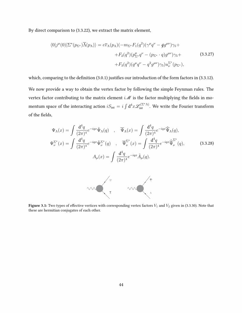
Figure 3.1: Two types of eective vertices with corresponding vertex factors V1 and V2 given in (3.3.30). Note thatthese are hermitian conjugates of each other.
44
We get the interaction action
iS(Σ∗Λ)int = ie
∫d4q1
(2π)4
d4q2
(2π)4
d4q3
(2π)4(2π)4δ(4)(q1 + q2 + q3)ΨΛ(q1)Aµ(q3)[
mΣ∗F1(q23)(γµqν3 − γα(q3)αg
µν)γ5 − F2(q23)(qµ2 q
ν3 − qα3 (q2)αg
µν)γ5+
+F3(q23)(qµ3 q
ν3 − qα3 (q3)αg
µν)γ5
]ΨΣ∗
ν (q2)+
+ie
∫d4q1
(2π)4
d4q2
(2π)4
d4q3
(2π)4(2π)4δ(4)(q1 + q2 + q3)Ψ
Σ∗
ν (q2)Aµ(q3)[mΣ∗F1(q2
3)(γµqν3 − γα(q3)αgµν)γ5 − F2(q2
3)(qµ2 qν3 − qα3 (q2)αg
µν)γ5+
+F3(q23)(qµ3 q
ν3 − qα3 (q3)αg
µν)γ5)]
ΨΛ(q1),
(3.3.29)
which gives rise to two types of vertices, depicted in Fig. 3.1. The expressions in the square
brackets in (3.3.29) are the corresponding vertex factors for the type-1 respective type-2 vertex,
explicitly
V µν1 = mΣ∗F1(q2
3)(γµqν3 − γα(q3)αgµν)γ5 − F2(q2
3)(qµ2 qν3 − qα3 (q2)αg
µν)γ5+
+ F3(q23)(qµ3 q
ν3 − qα3 (q3)αg
µν)γ5,
V µν2 = mΣ∗F1(q2
3)(γµqν3 − γα(q3)αgµν)γ5 − F2(q2
3)(qµ2 qν3 − qα3 (q2)αg
µν)γ5+
+ F3(q23)(qµ3 q
ν3 − qα3 (q3)αg
µν)γ5.
(3.3.30)
We note that the form of the two vertices is identical. The two types of vertices arise naturally
by demanding hermiticity of the Lagrangian. We chose here to distinguish the two for clarity
and for demonstration that the vertex factors really are identical. Having the vertex factors, we
may directly express any Feynman diagram with three-point interactions with no internal spinor
propagators.
45
Chapter 4
Cross section and decay rate
The link between theory and experiment in physics always relies on a correct translation from
the calculable to the measurable. The main measurable quantities in particle physics are cross
sections and decay rates. As already described in the introduction, these are the probabilities of
a reaction to occur. The constraints to a model very often is input from reality. By simplifying
the theory as much as possible, the parameters of the theory can be tted to experimental data.
In this way, the model becomes predictive.
In this section we will present the calculations of the amplitudes of two processes, both in a
one-photon approximation. Firstly, we calculate the dierential cross section of the scattering
e+e− → Σ∗Λ, a process which can already be measured at the electron-positron collider at BESIII
in Beijing [1]. Secondly, the dierential decay rate for the Dalitz decay Σ∗ → Λe+e− is calculated.
This process is planned to be performed at PANDA (proton-antiproton xed-target experiment)
[21] and HADES (proton-proton xed-target experiment) at the Facility for Antiproton and Ion
Research (FAIR) in Darmstadt [22]. We express the cross section and the decay rate in terms of
the three electromagnetic transition form factors for the Σ∗-Λ transition introduced in Chapter 3.
This theory input allows for a series of measurements to determine the form factors as functions
of the invariant mass q2 and in that way extract fundamental properties of these hyperons.
46
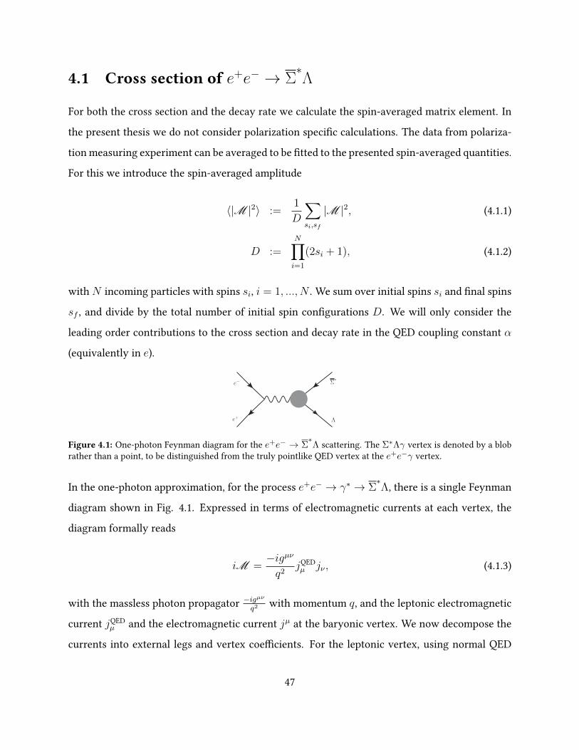
4.1 Cross section of e+e− → Σ∗Λ
For both the cross section and the decay rate we calculate the spin-averaged matrix element. In
the present thesis we do not consider polarization specic calculations. The data from polariza-
tion measuring experiment can be averaged to be tted to the presented spin-averaged quantities.
For this we introduce the spin-averaged amplitude
〈|M |2〉 :=1
D
∑si,sf
|M |2, (4.1.1)
D :=N∏i=1
(2si + 1), (4.1.2)
with N incoming particles with spins si, i = 1, ..., N . We sum over initial spins si and nal spins
sf , and divide by the total number of initial spin congurations D. We will only consider the
leading order contributions to the cross section and decay rate in the QED coupling constant α
(equivalently in e).
e−
e+
Σ∗
Λ
Figure 4.1: One-photon Feynman diagram for the e+e− → Σ∗Λ scattering. The Σ∗Λγ vertex is denoted by a blob
rather than a point, to be distinguished from the truly pointlike QED vertex at the e+e−γ vertex.
In the one-photon approximation, for the process e+e− → γ∗ → Σ∗Λ, there is a single Feynman
diagram shown in Fig. 4.1. Expressed in terms of electromagnetic currents at each vertex, the
diagram formally reads
iM =−igµνq2
jQEDµ jν , (4.1.3)
with the massless photon propagator −igµν
q2 with momentum q, and the leptonic electromagnetic
current jQEDµ and the electromagnetic current jµ at the baryonic vertex. We now decompose the
currents into external legs and vertex coecients. For the leptonic vertex, using normal QED
47
Feynman rules for the vertex coecient, we get
jµQED = eve+(pe+ , se+)γµue−(pe− , se−). (4.1.4)
Similarly, having the eective Lagrangian for the baryonic interactions, we use the vertex factor
from a type-1 vertex derived in (3.3.30) to get
jµ = euΛ(pΛ, sΛ)V µν1 vΣ∗
ν (pΣ∗ , sΣ∗), (4.1.5)
where we indicate the four-momentum and spin label for each particle.
From the momentum ow in each vertex we translate the Feynman rules (3.3.30) to
q3 → q , q2 → −pΣ∗ , q = pΣ∗ + pΛ (4.1.6)
The vertex factor is then
V µν1 (pΣ∗ , q) = mΣ∗F1(q2)(γµqν − /qgµν)γ5 + F2(q2)(pµΣ∗q
ν − (pΣ∗ · q)gµν)γ5+
+ F3(q2)(qµqν − q2gµν)γ5 =: −Γµν
R
(4.1.7)
where we introduce the vertex function with the subscript R, ΓµνR . The barred operation is dened
as
Γµν
:= γ0 (Γµν)† γ0. (4.1.8)
Similarly, we introduce the vertex function with subscript C denoting the evaluation of form
factors at their conjugate values,
Γµν
C := −mΣ∗F∗1 (q2)(γµqν − /qgµν)γ5 − F ∗2 (q2)(pµΣ∗q
ν − (pΣ∗ · q)gµν)γ5−
− F ∗3 (q2)(qµqν − q2gµν)γ5.(4.1.9)
48
By contracting indices we get the matrix element and the corresponding hermitian conjugate
M =e2
q2ve+(pe+ , se+)γµue−(pe− , se−)uΛ(pΛ, sΛ)Γ
µν
R vΣ∗
ν (pΣ∗ , sΣ∗),
M † =e2
q2(vΣ∗
ν (pΣ∗ , sΣ∗))†(Γ
µν
R )†u†Λ(pΛ, sΛ)u†e−(pe− , se−)ㆵv†e+(pe+ , se+) =
=e2
q2vΣ∗
ν (pΣ∗ , sΣ∗) γ0(Γµν
R )†γ0︸ ︷︷ ︸=ΓµνC
uΛ(pΛ, sΛ)ue−(pe− , se−)γµve+(pe+ , se+),
(4.1.10)
where we have introduced unity γ0γ0 = 1 and used γ0(γµ)†γ0 = γµ.
For the two incoming spin-12
particles, we get D = (212
+ 1)(212
+ 1) = 4. In the following, we
drop the trivial four-momentum argument and the spin argument for the spinors for convenience
and from (4.1.1) we have
〈|M |2〉 =e4
4q4
∑se− ,se+ ,sΣ∗ ,sΛ
(ve+γµue−uΛΓµν
R vΣ∗
ν )(vΣ∗
β ΓαβC uΛue−γαve+) =
=e4
4q4
∑se− ,se+ ,sΣ∗ ,sΛ
((ue−)j(γα)jk(ve+)k(ve+)m(γµ)mn(ue−)n)
((vΣ∗
β )a(ΓαβC )ab(uΛ)b(uΛ)c(Γ
µν
R )cd(vΣ∗
ν )d) =
=e4
4q4
∑se−
((ue−)n(ue−)j)(γα)jk∑se+
((ve+)k(ve+)m)(γµ)mn
∑sΣ∗
((vΣ∗
ν )d(vΣ∗
β )a)(ΓαβC )ab
∑sΛ
(uΛ)b(uΛ)c(Γµν
R )cd =
=−e4
4q4(/pe− +me)nj(γα)jk(/pe+ −me)km(γµ)mn
((/pΣ∗−mΣ∗)Pνβ)da(Γ
αβC )ab(/pΛ
+mΛ)bc(Γµν
R )cd =
=−e4
4q4Tr[(/pe− +me)γα(/pe+ −me)γµ]Tr[(/pΣ∗
−mΣ∗)PνβΓαβC (/pΛ+mΛ)Γ
µν
R ]
(4.1.11)
where in the second equality we explicitly write the spinor indices (denoted with latin letters) to
rewrite the expression in terms of traces. Lastly, we made use of the spin sum of spin-12
spinors
(2.1.10) and the vector-spinors (2.1.25).
49
We calculate the spin-averaged dierential cross section in the center of momentum frame given
in (2.3.8), where pe+ = −pe− and pΣ∗ = −pΛ. As customary for a 2→ 2 scattering process, the
Mandelstam variables are dened by
s := (pe− + pe+)2 = (pΣ∗ + pΛ)2 = q2,
t := (pe− − pΣ∗)2 = (pe+ − pΛ)2,
u := (pe− − pΛ)2 = (pe+ − pΣ∗)2.
(4.1.12)
We use the spin-averaged amplitude given in (4.1.11) which can be calculated in terms of the form
factors and their conjugates. We use the identity for the Mandelstam variables
s+ t+ u = m2e +m2
e +m2Σ∗ +m2
Λ (4.1.13)
to reduce the expression from three kinematic variables s, t, u to only s, t. A direct calculation of
the spin-averaged amplitude shows that the expression contains mixed terms of the three form
factorsFi(q2). In the following we will dene three new linear combinations of these form factors
in order for the amplitude to exclude any mixed terms of form factors.
We will treat the cross section as a bilinear form, by dening
F(q2) :=
F1(q2)
F2(q2)
F3(q2)
, F†(q2) =(F ∗1 (q2), F ∗2 (q2), F ∗3 (q2)
)(4.1.14)
and a matrix A(q2, t) such that
(dσdΩ
)CM
(q2, t) = F†(q2)A(q2, t)F(q2). (4.1.15)
By calculation of the amplitude, one sees thatA (with real entries) is symmetric,AT = A, however
50
not diagonal. Such a bilinear form can be brought to a quadratic form
(dσdΩ
)CM
(q2, t) = G†(q2)D(q2, t)G(q2), (4.1.16)
where we dene a change of basis to a new set of form factors
G(q2) :=
G+1(q2)
G0(q2)
G−1(q2)
, G†(q2) =(G∗+1(q2), G∗0(q2), G∗−1(q2)
), (4.1.17)
by the transformation
G(q2) = T(q2) · F(q2) ⇔ F(q2) = T−1(q2)G(q2), (4.1.18)
for some transformation matrix T(q2) ∈M3×3(C), such that the matrix D(q2, t) is now diagonal,
(dσdΩ
)CM
= G†(q2)(T−1(q2)
)†A(q2, t)T(q2)︸ ︷︷ ︸=D(q2,t)
G(q2). (4.1.19)
Such a diagonalized form can be achieved by the transformation matrix
T(q2) =
mΣ∗(mΣ∗ +mΛ) 1
2(m2
Σ∗ −m2Λ + q2) q2
m2Σ∗ m2
Σ∗12(m2
Σ∗ −m2Λ + q2)
−mΛ(mΣ∗ +mΛ) + q2 12(m2
Σ∗ −m2Λ + q2) q2
(4.1.20)
with the inverse
T−1(q2) =
1
(mΣ∗+mΛ)2−q2 0 −1(mΣ∗+mΛ)2−q2
2(−m2Λ+mΣ∗mΛ+q2)
λ(q2,m2Σ∗ ,m
2Λ)
−4q2
λ(q2,m2Σ∗ ,m
2Λ)
2(m2Σ∗−mΣ∗mΛ)
λ(q2,m2Σ∗ ,m
2Λ)
−2m2Σ∗
λ(q2,m2Σ∗ ,m
2Λ)
2(−m2Λ+m2
Σ∗+q2)
λ(q2,m2Σ∗ ,m
2Λ)
−2m2Σ∗
λ(q2,m2Σ∗ ,m
2Λ)
, (4.1.21)
51
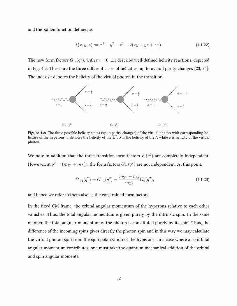
and the Källén function dened as
λ(x, y, z) := x2 + y2 + z2 − 2(xy + yz + zx). (4.1.22)
The new form factors Gm(q2), with m = 0,±1 describe well-dened helicity reactions, depicted
in Fig. 4.2. These are the three dierent cases of helicities, up to overall parity changes [23, 24].
The index m denotes the helicity of the virtual photon in the transition.
σ = 32 σ = 1
2σ = −1
2
λ = 12 λ = 1
2 λ = 12
ρ = 1 ρ = 0 ρ = −1
G+1(q2) G0(q
2) G−1(q2)
Figure 4.2: The three possible helicity states (up to parity changes) of the virtual photon with corresponding he-licities of the hyperons; σ denotes the helicity of the Σ
∗, λ is the helicity of the Λ while ρ is helicity of the virtualphoton.
We note in addition that the three transition form factors Fi(q2) are completely independent.
However, at q2 = (mΣ∗ +mΛ)2, the form factors Gm(q2) are not independent. At this point,
G+1(q2) = G−1(q2) =mΣ∗ +mΛ
mΣ∗G0(q2), (4.1.23)
and hence we refer to them also as the constrained form factors.
In the xed CM frame, the orbital angular momentum of the hyperons relative to each other
vanishes. Thus, the total angular momentum is given purely by the intrinsic spin. In the same
manner, the total angular momentum of the photon is constituted purely by its spin. Thus, the
dierence of the incoming spins gives directly the photon spin and in this way we may calculate
the virtual photon spin from the spin polarization of the hyperons. In a case where also orbital
angular momentum contributes, one must take the quantum mechanical addition of the orbital
and spin angular momenta.
52
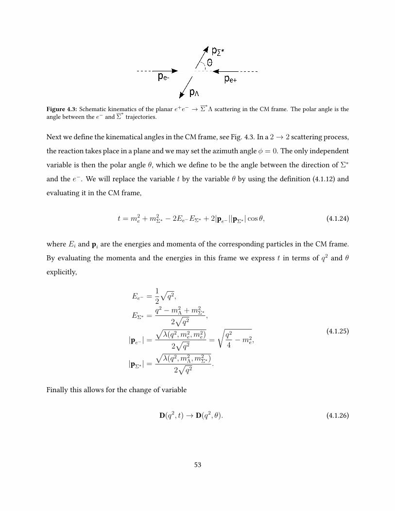
Figure 4.3: Schematic kinematics of the planar e+e− → Σ∗Λ scattering in the CM frame. The polar angle is the
angle between the e− and Σ∗ trajectories.
Next we dene the kinematical angles in the CM frame, see Fig. 4.3. In a 2→ 2 scattering process,
the reaction takes place in a plane and we may set the azimuth angle φ = 0. The only independent
variable is then the polar angle θ, which we dene to be the angle between the direction of Σ∗
and the e−. We will replace the variable t by the variable θ by using the denition (4.1.12) and
evaluating it in the CM frame,
t = m2e +m2
Σ∗ − 2Ee−EΣ∗ + 2|pe−||pΣ∗| cos θ, (4.1.24)
where Ei and pi are the energies and momenta of the corresponding particles in the CM frame.
By evaluating the momenta and the energies in this frame we express t in terms of q2 and θ
explicitly,
Ee− =1
2
√q2,
EΣ∗ =q2 −m2
Λ +m2Σ∗
2√q2
,
|pe−| =√λ(q2,m2
e,m2e)
2√q2
=
√q2
4−m2
e,
|pΣ∗| =√λ(q2,m2
Λ,m2Σ∗)
2√q2
.
(4.1.25)
Finally this allows for the change of variable
D(q2, t)→ D(q2, θ). (4.1.26)
53
The nal expression for the dierential cross section is then,
(dσdΩ
)CM
(q2, θ) =|pΣ∗ ||pe−|
e4
384π2q4(q2 − (mΣ∗ −mΛ)2)((
(1 + cos2 θ) + 4m2e
q2sin2 θ
)(3|G+1(q2)|2 + |G−1(q2)|2)+
+ 4
(4m2e
m2Σ∗
cos2 θ +q2
m2Σ∗
sin2 θ
)|G0(q2)|2
).
(4.1.27)
In regions of the invariant mass which are physical, the electron mass is negligible m2e q2 as
well as compared to the hyperon mass m2e m2
Σ∗ . In the limit me → 0, the dierential cross
section simplies to the expression
(dσdΩ
)CM
(q2, θ) =√λ(q2,m2
Σ∗ ,m2Λ)
e4
384π2q6(q2 − (mΣ∗ −mΛ)2)(
(1 + cos2 θ)(3|G+1(q2)|2 + |G−1(q2)|2) +4q2
m2Σ∗
sin2 θ|G0(q2)|2),
(4.1.28)
where we also entered the three-momentum of the electron in the zero electron mass limit,
|pe− | →√q2
2. (4.1.29)
This result can be compared to the results presented for a dierential cross section for e+e−
annihilation into baryon and anitbaryon pairs by Körner and Kuroda [24]. The general expression
for the dierential cross section that they predict for such a reaction is
dσd(cos θ)
∝∑λ
(1
2(1 + cos2 θ)(|Γλ+1,λ(q2)|2 + |Γλ−1,λ(q2)|2) + sin2 θ|Γλ,λ(q2)|2
), (4.1.30)
with the solid angle dierential dΩ related to the polar angle dierential dθ by dΩ = dφd(cos θ),
with φ being the azimuth angle over which the expression can be integrated over. The helicity
amplitudes Γσ,λ(q2) used in this expression are linear in the constrained form factors Gm(q2)
54
according to
|G−1(q2)|2|G+1(q2)|2 = 3
|Γ 12,− 1
2 (q2)|2|Γ 3
2, 12 (q2)|2
,
|G0(q2)|2|G+1(q2)|2 =
3
2
m2Σ∗
q2
|Γ 12, 12 (q2)|2
|Γ 32, 12 (q2)|2
.
(4.1.31)
With these relations between the helicity amplitudes and the form factors, the expression (4.1.30)
and our derived expression (4.1.28) are the same, up to kinematical coecients. It is possible to
check that also the kinematical coecients match up.
4.2 Decay rate of Σ∗ → Λe+e−
We consider now the Dalitz decay Σ∗ → Λγ∗ → Λe+e− in the one-photon approximation. The
single Feynman diagram which contributes to the amplitude is shown in Fig. 4.4. The vertex
again is a vertex of type-1 from (3.3.30), which now translates by the replacement
q3 → −q , q2 → pΣ∗ , q = pΣ∗ − pΛ (4.2.1)
to the vertex factor
V µν1 (pΣ∗ , q) = −mΣ∗F1(q2)(γµqν − /qgµν)γ5 + F2(q2)(pµΣ∗q
ν − (pΣ∗ · q)gµν)γ5+
+ F3(q23)(qµqν − q2gµν)γ5 = Γµν(pΣ∗ , q).
(4.2.2)
We dene Mandelstam variables by
s : = (pΣ∗ − pΛ)2 = (pe+ + pe−)2 = q2,
t : = (pΣ∗ − pe+)2 = (pΛ + pe−)2,
u : = (pΣ∗ − pe−)2 = (pΛ + pe+)2.
(4.2.3)
In the same manner as for the cross section, the full matrix element for the decay is given by the
55
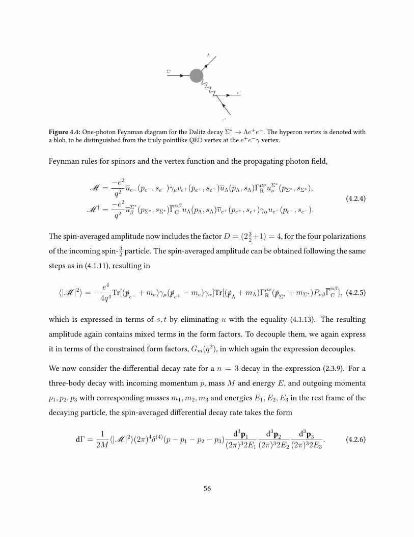
Σ∗
Λ
e+
e−
Figure 4.4: One-photon Feynman diagram for the Dalitz decay Σ∗ → Λe+e−. The hyperon vertex is denoted witha blob, to be distinguished from the truly pointlike QED vertex at the e+e−γ vertex.
Feynman rules for spinors and the vertex function and the propagating photon eld,
M =−e2
q2ue−(pe− , se−)γµve+(pe+ , se+)uΛ(pΛ, sΛ)ΓµνR uΣ∗
ν (pΣ∗ , sΣ∗),
M † =−e2
q2uΣ∗
β (pΣ∗ , sΣ∗)Γαβ
C uΛ(pΛ, sΛ)ve+(pe+ , se+)γαue−(pe− , se−).
(4.2.4)
The spin-averaged amplitude now includes the factorD = (232+1) = 4, for the four polarizations
of the incoming spin-32
particle. The spin-averaged amplitude can be obtained following the same
steps as in (4.1.11), resulting in
〈|M |2〉 = − e4
4q4Tr[(/pe− +me)γµ(/pe+ −me)γα]Tr[(/pΛ
+mΛ)ΓµνR (/pΣ∗+mΣ∗)PνβΓ
αβ
C ], (4.2.5)
which is expressed in terms of s, t by eliminating u with the equality (4.1.13). The resulting
amplitude again contains mixed terms in the form factors. To decouple them, we again express
it in terms of the constrained form factors, Gm(q2), in which again the expression decouples.
We now consider the dierential decay rate for a n = 3 decay in the expression (2.3.9). For a
three-body decay with incoming momentum p, mass M and energy E, and outgoing momenta
p1, p2, p3 with corresponding masses m1,m2,m3 and energies E1, E2, E3 in the rest frame of the
decaying particle, the spin-averaged dierential decay rate takes the form
dΓ =1
2M〈|M |2〉(2π)4δ(4)(p− p1 − p2 − p3)
d3p1
(2π)32E1
d3p2
(2π)32E2
d3p3
(2π)32E3
. (4.2.6)
56
It is customary to dene the following Lorentz scalars,
m212 := (p1 + p2)2 , m2
23 := (p2 + p3)2, (4.2.7)
which nally yields the double-dierential decay rate in the rest frame of the decaying particle,
d2Γ
dm212dm2
23
=1
32M3(2π)3〈|M |2〉. (4.2.8)
We may rewrite this in a Lorentz invariant way by noting that M =√p2, and upon replacing,
the expression becomes manifestly Lorentz invariant (the amplitude being a Lorentz scalar),
d2Γ
dm212dm2
23
=1
32(p2)3/2(2π)3〈|M |2〉, (4.2.9)
with the limits
(m1 +m2)2 ≤ m212 ≤ (M −m3)2
(m223)par ≤ m2
23 ≤ (m223)apar,
(4.2.10)
with the latter limits being the cases when the directions of the particles 2 and 3 are parallel
respective antiparallel in the CM frame of particles 1 and 2,
(m223)par = (E2 + E3)2 −
(√E2
2 −m22 +
√E2
3 −m23
)2
,
(m223)apar = (E2 + E3)2 −
(√E2
2 −m22 −
√E2
3 −m23
)2
,
(4.2.11)
with the energies E2, E3 now expressed in the CM frame of particles 1 and 2.
We consider the decay rate in the CM rest frame where particle 1 is the electron, and particle 2 is
the positron, in which casepe− = −pe+ , pΣ∗ = pΛ. In this frame, the decay is planar, and we may
dene our coordinate system as in Fig. 4.5, where we dene the angle θ between the direction of
the electron and the Λ (or Σ∗).
57
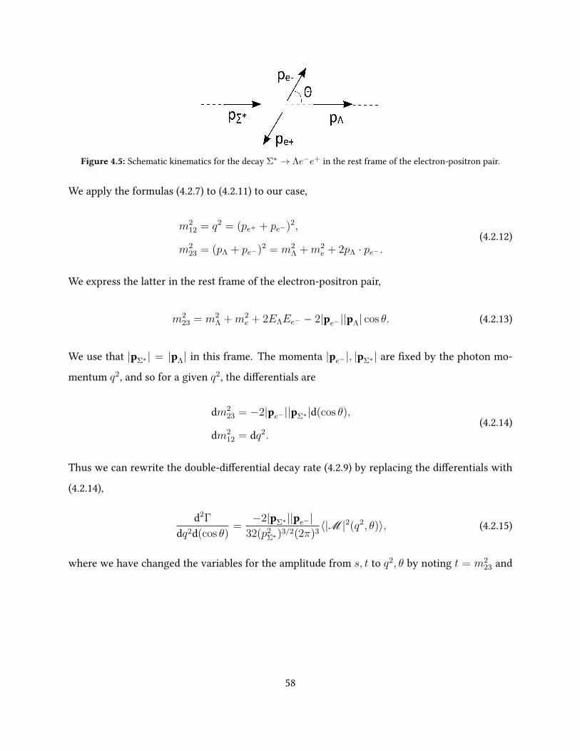
Figure 4.5: Schematic kinematics for the decay Σ∗ → Λe−e+ in the rest frame of the electron-positron pair.
We apply the formulas (4.2.7) to (4.2.11) to our case,
m212 = q2 = (pe+ + pe−)2,
m223 = (pΛ + pe−)2 = m2
Λ +m2e + 2pΛ · pe− .
(4.2.12)
We express the latter in the rest frame of the electron-positron pair,
m223 = m2
Λ +m2e + 2EΛEe− − 2|pe−||pΛ| cos θ. (4.2.13)
We use that |pΣ∗ | = |pΛ| in this frame. The momenta |pe−|, |pΣ∗| are xed by the photon mo-
mentum q2, and so for a given q2, the dierentials are
dm223 = −2|pe− ||pΣ∗|d(cos θ),
dm212 = dq2.
(4.2.14)
Thus we can rewrite the double-dierential decay rate (4.2.9) by replacing the dierentials with
(4.2.14),
d2Γ
dq2d(cos θ)=−2|pΣ∗||pe− |
32(p2Σ∗)
3/2(2π)3〈|M |2(q2, θ)〉, (4.2.15)
where we have changed the variables for the amplitude from s, t to q2, θ by noting t = m223 and
58
using (4.2.13) to express t in terms of θ. Using the result for the amplitude (4.2.5) we obtain
d2Γ
dq2d(cos θ)=
1
(2π)3
e4|pΣ∗ ||pe−|96m3
Σ∗q2
(q2 − (mΣ∗ −mΛ)2)[((1 + cos2 θ + 4
m2e
q2sin2 θ
)(3|G+1(q2)|2 + |G−1(q2)|2)+
+ 4
(q2
m2Σ∗
sin2 θ + 4m2e
m2Σ∗
cos2 θ
)|G0(q2)|2
],
(4.2.16)
with the momenta of the Σ∗ and the electron given in the rest frame of the electron-positron pair,
and given in terms of q2 by
|pe−| =
√q2
4−m2
e, (4.2.17)
|pΣ∗| =
√λ(q2,m2
Σ∗ ,m2Λ)
2√q2
. (4.2.18)
One should note that in the given decay the invariant mass q2 is limited in the kinematical region
4m2e ≤ q2 ≤ (mΣ∗ −mΛ)2 (4.2.19)
and so the factor q2− (mΣ∗−mΛ)2 is always non-positive. However we note that the integration
in m223 goes from the parallel to antiparallel constellation of the momenta of Σ∗ and e−, which
corresponds to cos θ going from 1 to−1, which is minus that of usual integration. In the integral
given above one must consider that the integration limits are interchanged and so the total decay
rate will indeed be positive as is physical.
A good approximation again is made for m2e q2 and m2
e m2Σ∗ , in which case we obtain
d2Γ
dq2d(cos θ)=√λ(q2,m2
Σ∗ ,m2Λ)
1
(2π)3
e4
392m3Σ∗q
2(q2 − (mΣ∗ −mΛ)2)[
(1 + cos2 θ)(3|G+1(q2)|2 + |G−1(q2)|2) +4q2
m2Σ∗
sin2 θ|G0(q2)|2].
(4.2.20)
The vanishing-electron-mass approximation can lead to issues when obtaining the total decay
59
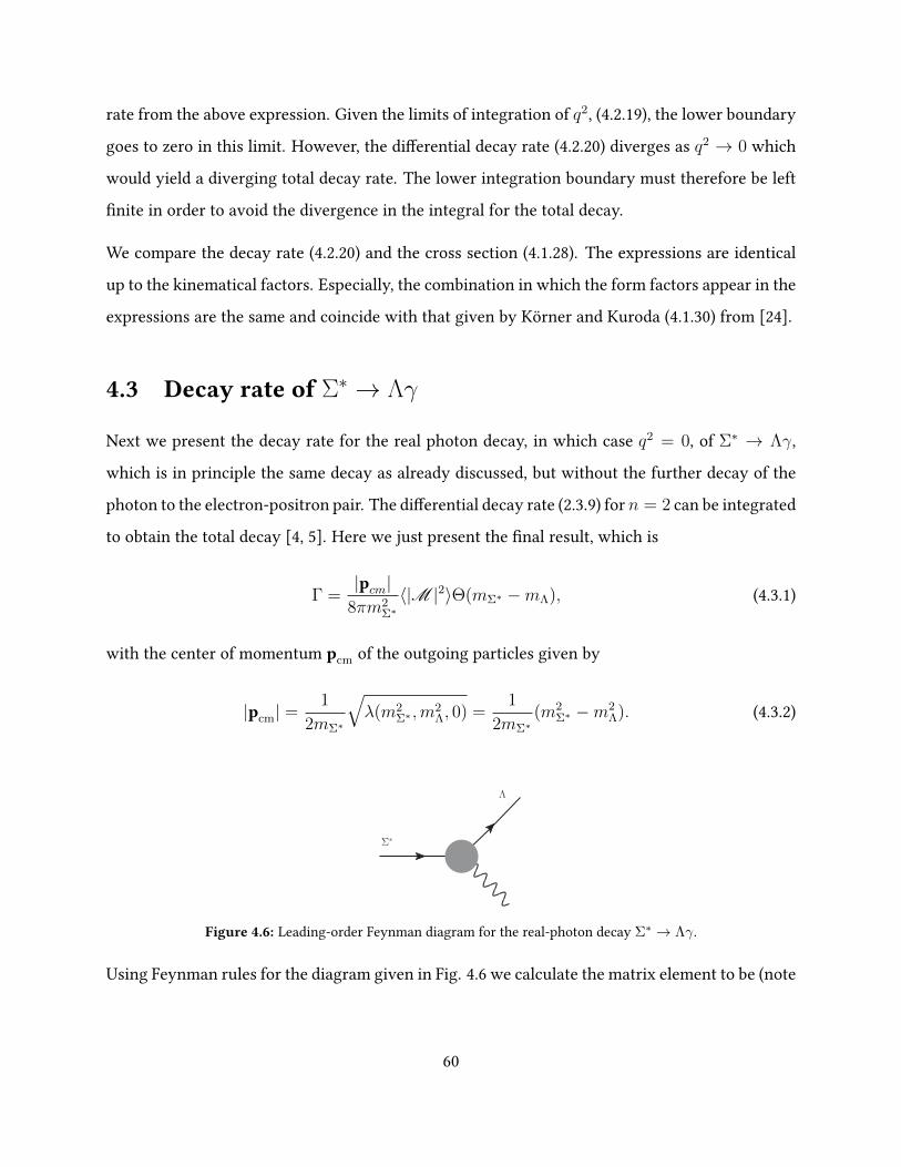
rate from the above expression. Given the limits of integration of q2, (4.2.19), the lower boundary
goes to zero in this limit. However, the dierential decay rate (4.2.20) diverges as q2 → 0 which
would yield a diverging total decay rate. The lower integration boundary must therefore be left
nite in order to avoid the divergence in the integral for the total decay.
We compare the decay rate (4.2.20) and the cross section (4.1.28). The expressions are identical
up to the kinematical factors. Especially, the combination in which the form factors appear in the
expressions are the same and coincide with that given by Körner and Kuroda (4.1.30) from [24].
4.3 Decay rate of Σ∗ → Λγ
Next we present the decay rate for the real photon decay, in which case q2 = 0, of Σ∗ → Λγ,
which is in principle the same decay as already discussed, but without the further decay of the
photon to the electron-positron pair. The dierential decay rate (2.3.9) for n = 2 can be integrated
to obtain the total decay [4, 5]. Here we just present the nal result, which is
Γ =|pcm|
8πm2Σ∗〈|M |2〉Θ(mΣ∗ −mΛ), (4.3.1)
with the center of momentum pcm of the outgoing particles given by
|pcm| =1
2mΣ∗
√λ(m2
Σ∗ ,m2Λ, 0) =
1
2mΣ∗(m2
Σ∗ −m2Λ). (4.3.2)
Σ∗
Λ
Figure 4.6: Leading-order Feynman diagram for the real-photon decay Σ∗ → Λγ.
Using Feynman rules for the diagram given in Fig. 4.6 we calculate the matrix element to be (note
60
that the baryonic vertex is exactly the same as for the Dalitz decay)
M = −ieuΛ(pΛ, sΛ)ΓµνR uΣ∗
ν (pΣ∗ , sΣ∗)ε∗µ(q, sγ),
M † = ieεα(q, sγ)uΣ∗
β (pΣ∗ , sΣ∗)Γαβ
C uΛ(pΛ, sΛ),(4.3.3)
with polarization vector εµ(q, sγ) for the photon with corresponding momentum and spin. The
spin-averaged amplitude (D = 4 again for the three polarizations of spin for the incoming Σ∗),
again suppressing the trivial momenta and spin arguments of the spinors and polarization vector
is
〈|M |2〉 =e2
4
∑sγ
ε∗µεα︸ ︷︷ ︸=−gµα
∑sΣ∗ ,sΛ
uΛΓµνR uΣ∗
ν uΣ∗
β Γαβ
C uΛ =
=e2
4Tr[gµα(/pΛ
+mΛ)ΓµνR (/pΣ∗+mΣ∗)PνβΓ
αβ
C ],
(4.3.4)
where we used the spin sum of polarization vectors (2.1.22). Using this result in the full decay
rate (4.3.1) nally gives (the step function being non-zero as mΣ∗ > mΛ),
Γ =e2(m2
Σ∗ −m2Λ)
96πm3Σ∗
(mΣ∗ −mΛ)2[3|G+1(0)|2 + |G−1(0)|2
]. (4.3.5)
We note a relevancy check for the result (4.3.5). The on-shell photon has only two polarizations
(helicities ±1), and thus we expect the decay rate of this reaction to not include the form factor
G0(0), the form factor corresponding to the photon of helicity 0.
According to the Particle Data Group values given for the total decay width of the Σ∗ given in
(2.4.1) and the branching ratio in the real-photon decay, given in (2.4.2), the experimental value
for this decay width is Γ = 0.45 MeV. In practice, this decay serves the purpose of tting of input
parameters to experimental data. In the preliminary work presented in Chapter 6, the parameters
from the chiral Lagrangian are tted such that the form factors at the real-photon point reproduce
the total decay width of the Σ∗ → Λγ decay.
61
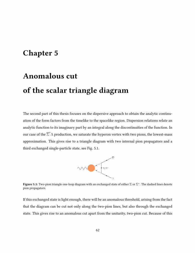
Chapter 5
Anomalous cut
of the scalar triangle diagram
The second part of this thesis focuses on the dispersive approach to obtain the analytic continu-
ation of the form factors from the timelike to the spacelike region. Dispersion relations relate an
analytic function to its imaginary part by an integral along the discontinuities of the function. In
our case of the Σ∗Λ production, we saturate the hyperon vertex with two pions, the lowest-mass
approximation. This gives rise to a triangle diagram with two internal pion propagators and a
third exchanged single-particle state, see Fig. 5.1.
Σ∗
Λ
Σ/Σ∗
Figure 5.1: Two-pion triangle one-loop diagram with an exchanged state of either Σ or Σ∗. The dashed lines denotepion propagators.
If this exchanged state is light enough, there will be an anomalous threshold, arising from the fact
that the diagram can be cut not only along the two-pion lines, but also through the exchanged
state. This gives rise to an anomalous cut apart from the unitarity, two-pion cut. Because of this
62
anomalous piece, the analytic structure of the discontinuities needs some careful examination. In
this chapter, the scalar one-loop triangle diagram is considered as a model to examine how the
analytic structure works for the real triangle diagram. As the scalar diagram can be calculated
directly, the procedure is to compare the direct calculation to the calculation with aid of dispersion
relations. In this manner we examine to which extent the dispersive analysis works. The direct
calculation is done based on the steps by ’t Hooft and Veltman [25]. Firstly we present some
prerequisites needed for the following work. For more thorough background on the topic, the
reader is referred to Peskin and Schroeder [5], Gamelin [26], as well as other textbooks on complex
analysis and analyticity of amplitudes. We will rst dene what is meant by a cut of a diagram;
what are the unitarity and the anomalous cuts; present unsubtracted and subtracted dispersion
relations; and introduce Riemann surfaces.
5.1 Prerequisites and denitions
We will here present the basic background needed to perform the calculations at hand. Firstly
we consider dispersion relations for analytic functions, then present the Cutkosky cutting rules,
and nally introduce Riemann sheets arising from discontinuity cuts.
5.1.1 Dispersion relations
In the following, we will be concerned with scattering amplitudes as functions of the invariant
mass in a given reaction. Considering production processes, the invariant mass q2 of the photon
will correspond to the s-channel exchange, and q2 = s. This leads to an examination of the s-
channel matrix element M (s), and therefore also the form factors Fi(s). The reactions at hand
have a threshold energy for which the intermediate states can go on-shell. The amplitude with
loops contains factors of the form
∝ 1
p2 −m2 + iε, (5.1.1)
63
with innitesimal ε > 0. When p2 6= m2, the imaginary part is suppressed, however when the
on-shell condition p2 = m2 is satised, the imaginary part becomes important, and the amplitude
obtains also an imaginary part, while for energies below the threshold, the amplitude is real. This
physical input motivates the following short mathematical introduction, where we develop how
to deal with functions of this type.
As an example, we will consider a model function f(z) : C→ C, which is analytic in the upper
half complex z-plane, and obtains real values on the real axis. Along the line [z0,∞) the function
has a discontinuity. On the real line,
f(z) = f(z∗)∗. (5.1.2)
If f(z) is analytic, then so is f(z∗)∗, which can be checked by direct usage of the Cauchy-Riemann
equations [26]. The above then constitutes the analytic continuation of the function f(z) to the
entire complex plane. By continuity, the function must satisfy the same condition (5.1.2) for
values slightly above this interval, with imaginary parts ε,
f(z + iε) = f(z − iε)∗ ↔
Ref(z + iε) = Ref(z − iε),
Imf(z + iε) = −Imf(z − iε).(5.1.3)
This is referred to as the Schwarz’s reection principle [26, 27] and shows the discontinuous
behavior of the function on the line segment z > z0. We dene the discontinuity at every point
on this line of discontinuity as the dierence between the values above and below the real axis,
discf(z) := f(z + iε)− f(z − iε) = 2i Imf(z + iε), (5.1.4)
where we use the condition (5.1.3) for the equality. This is sometimes referred to as the spectral
theorem [27].
In the case of general cuts in the complex plane, not only on the real axis, the prescription f(z±iε)is not useful. Such is the case for the anomalous cut discussed later. We consider generally the
64
function evaluated on the left, f(z)+, and right, f(z)−, of the discontinuity, which has well-
dened direction in an integration contour. For z along the cut, the discontinuity is then
discf(z) := f(z)+ − f(z)−. (5.1.5)
The real and imaginary parts of an analytic function are not independent, but are correlated with
an integral expression called the dispersion relations [28]. When also discussing anomalous cuts,
we will present a short proof of the dispersion relations in Section 5.4.2. For now we state the
relation for the function f(z) with a branch cut Br = [z0,∞),
f(z) =1
π
∫Br
dz′Imf(z′)
z′ − z , (5.1.6)
which holds if the integrand part Imf(z)→ 0 as |z| → ∞.
It may happen that the integral above does not converge at innity. When such convergence
does not occur, the above dispersion relation does not hold for the function, but it may hold for
its derivative (or any order of derivative if the rst order fails to hold, but the argumentation
follows in the same manner),
f ′(z) =1
π
∫Br
dz′Imf ′(z′)z′ − z . (5.1.7)
By integrating the right-hand side by parts, (and noting Imf ′(z) = ddz Imf(z)),
f ′(z) =1
π
Imf(z)
z′ − z
∣∣∣∣∞z0
+1
π
∫Br
dz′Imf(z′)
(z′ − z)2. (5.1.8)
By assumption, the imaginary part vanishes at the boundaries z0 and∞ of the cut Br, in which
case we drop the rst term. Finally, we integrate both sides of (5.1.8) between some nite point
65
z1 and z, and changing the order of integration in the variables z′ and z,
∫ z
z1
dzf ′(z) =1
π
∫ z
z1
dz∫Br
dz′Imf(z′)
(z′ − z)2,
⇒ f(z)− f(z1) =1
π
∫Br
dz′∫ z
z1
dzImf(z′)
(z′ − z)2,
⇒ f(z)− f(z1) =1
π
∫Br
(Imf(z′)
z′ − z −Imf(z′)
z′ − z1
).
(5.1.9)
By rearranging we nally get the once-subtracted dispersion relation for f(z) at the point z1,
f(z) = f(z1) +z − z1
π
∫Br
Imf(z′)
(z′ − z)(z′ − z1). (5.1.10)
The procedure can be formulated for the nth derivative of f(z), in which case we formulate the
n-times subtracted dispersion relation at the point z1,
f(z) = f(z1) +n−1∑i=1
Ai(z − z1)i +(z − z1)n
π
∫I
dz′Imf(z′)
(z′ − z)(z′ − z1)n. (5.1.11)
Subtractions introduce the constants Ai which in practice are parameters of a model which need
to be determined experimentally. Higher subtractions suppress the potential problem with con-
vergence of an integral, as it introduces higher powers of the integrated variable in the denomi-
nator. However, higher subtractions mean also more parameters to be tted to experimental data.
In practice one nds the optimal choice and investigates how well dierent orders of subtractions
reproduce data.
5.1.2 Cutkosky cutting rules
We now present one more very useful tool which we use for our calculations. These are the
Cutkosky cutting rules, which provide an easy way to evaluate the imaginary parts of diagrams
[5, 29, 30].
As discussed earlier, amplitudes become imaginary when internal propagators satisfy the on-
66
shell condition. Away from the on-shell condition, the iε in the propagators are neglected and
the amplitudes have no imaginary parts. Cutkosky showed that the imaginary part of a loop
diagram is given by cutting it with lines in all possible ways which allow the cut propagators
to go on-shell such that the diagram is divided into two disjoint parts. The discontinuity of the
function, which is related to the imaginary part, is then the sum of all these cut diagrams.
Consider an integral over propagators
I =
∫Dk
m∏i
1
p2i −m2
i + iε, (5.1.12)
where Dk is the integral over all loop momenta. The discontinuity is obtained by cutting the
diagram into two, in a way that the cut propagators can be on-shell. The cut internal edges
are replaced by positive delta functions, while all other internal edges are left unchanged. Let
i = 1, ..., n label the n internal edges which are cut, and the j = n + 1, ...,m edges which are
not cut, in a diagram with m propagators. The momenta of each internal exchange particle are
pi and mass mi. Then we replace the propagator factor accordingly,
1
p2i −m2
i + iε→ −2πiδ+(p2
i −m2i ) for i = 1, ..., n,
1
p2j −m2
j + iε→ 1
p2j −m2
j + iεfor j = n+ 1, ...,m,
(5.1.13)
where we introduce the positive delta function as δ+(p2i − m2
i ) = δ(p2i − m2
i )Θ(p0i ) in order
to retain the correct energy ow in the diagram, according to notation used in [27, 30]. The
discontinuity is then given by
discI =∑
possible cuts
∫Dk
n∏i=1
(−2πi)δ+(p2i −m2
i )m∏
j=n+1
1
p2j −m2
j + iε= 2i ImI, (5.1.14)
where we sum over all possible cut diagrams. This expression will be used later to obtain the
unitarity cut of the scalar triangle diagram.
67
5.1.3 Riemann surfaces and cuts
As known from complex analysis, complex and multivalued functions give rise to Riemann sheets
when dening them to be continuous [26]. We consider here the logarithm function g : C→ C,
g(z) = log(z) := w ∈ C|exp(w) = z, (5.1.15)
which can elegantly be rewritten as the set
log(z) = log|z|+ iArgz + n2πi, n ∈ Z, (5.1.16)
dening the principal argument as Argz ∈ [−π, π). One denes single-valued functions by
setting n x, called the nth branch of the logarithm,
Logn(z) := log|z|+ iArgz + n2πi. (5.1.17)
These are continuous on the cut plane C\(−∞, 0], the negative real axis being the branch cut
and the z = 0 being the branch point. The discontinuity on the negative real axis implies that
for real and positive x,
Logn(−x+ iε) 6= Logn(−x− iε) , ε→ 0. (5.1.18)
One now denes instead of the complex z-plane, a Riemann surface on which the logarithm
function is in fact continuous. In this notion, there is an analytic continuation through the branch
cut in a way that the continuation is to the next branch of the logarithm. In this sense,
Log0(−x+ iε) = Log1(−x− iε) = Log0(−x+ iε) + 2πi, (5.1.19)
68
and in a similar manner for any other branch. The term 2πi is the discontinuity of the logarithm
function at the branch cut,
disc Log(−x) = Log(−x− iε)− Log(−x+ iε) = 2πi, (5.1.20)
or using the notation used in (5.1.5) for the left and right side of a discontinuity running from 0
to innity,
disc Log(−x) = Log(−x)+ − Log(−x)−. (5.1.21)
A more complicated function will also have a more subtle discontinuity. In the same manner one
may dene Riemann sheets, the branch cut and discontinuities over the cut. The position of the
branch point is given unambiguously by the function, while the branch cut is chosen arbitrarily.
The shape and structure of the Riemann sheet stays unchanged, but the choice of the position of
the discontinuous segment may change.
5.1.4 Exchange states in the two-pion one-loop diagram
The hyperon-photon vertex is divided into two parts, with an intermediate state. The intemediate
state are any Goldstone boson states which conserve all quantum numbers. In a full expansion,
one should consider all possible intermediate states. However, in the low-energy regime in which
we are working in, we make an approximation that only the lowest-mass states are excited. The
conservation of angular momentum, parity and isospin leads to the situation that the only pos-
sible such states are even number of pions. In this work we approximate it with the very lowest
energy case, the two-pion excitation. This approximation is also made in [2]. In Chapter 6 we ex-
amine the diagram in more detail. If interested at this point, the reader is referred to this chapter.
The nal result which contributes to an anomalous threshold is the triangle diagram in Fig. 5.1.
This is a triangle diagram in a t- and u-channel (however in Fig. 5.1 we depict only the t-channel)
with an exchanged hyperon and two pion propagators. Without taking the conservation of quan-
69
tum numbers into consideration, any hyperon exchange state is allowed. Adding on the dierent
quantum numbers, we reduce the possible hyperons to only two possible ones. Firstly, we con-
sider the conservation of electric charge, As the incoming hyperons have neutral electric charge,
a neutral exchange particle would need neutral pions exchanged in the triangle loop which couple
directly to a photon. However two identical particles (being each others antiparticles) connected
to a photon violates charge conjugation. Such a coupling term in the Lagrangian would transform
under charge conjugation as
π0π0AµC−→ −π0π0Aµ, (5.1.22)
violating charge conjugation invariance.
Next, the exchange particle must have a nonzero strangeness number, carrying the strangeness
current between the two external hyperons, as the pions have strangeness number 0. Further, it
needs to have baryon number 1, as this otherwise would violate the baryon number conservation
at the vertices.
The two particles lowest in mass which satisfy the above are the Σ+ and the Σ∗+. Their masses
are given in Tabs. 2.2 and 2.3. In the calculation of the amplitudes, we will consider both of these
exchanged states in the t- and u-channel.
The triangle loop has been analyzed for three scalar elds by Karplus et al. [20] for certain con-
straint on the masses of the incoming particles. In this paper [20], the mass condition for a particle
to be able to decay into the loop particle, is presented. For certain values of the external and in-
ternal masses, the state in the exchanged channel (t- or u-channel) may be on-shell and therefore
contribute to the imaginary part of the diagram, according to the Cutkosky cutting rules. This
gives rise to an anomalous cut in addition to the unitarity cut. The denition of the unitarity cut
will be presented below. Following the general formula prescribed by Karplus, the anomalous cut
for our triangle loop can be obtained for an exchange particle with mass mex which satises
m2ex <
1
2(m2
Σ∗ +m2Λ − 2m2
π). (5.1.23)
70
For our case, the mass of the Σ∗+ is too large to satisfy (5.1.23), whereas the mass of Σ+ does
satisfy it. We will drop the charge superscript of the octet and decuplet exchange hyperons for
convenience in later use. We will see in the next section explicitly that the Σ∗ exchange does not
need an addition of an anomalous cut for the dispersion relations, while the Σ exchange does.
With the triangle diagram at hand, we notice that one can cut, according to Cutkosky cutting
rules, along the two pion lines, as this is energetically possible for certain energies. Such a cut
with an intermediate state of light particles is always possible and yields the unitarity cut of a
diagram. The on-set of the unitarity cut for the two-pion case is at s = 4m2π, the energy at which
the two pions can go on-shell, and hence we refer to this cut as the two-pion unitarity cut. In
principle, one might also consider heavier excitations (which is not performed in this work), for
example a four-pion state, in which case the on-set would be the rest mass of the four pions.
This also constitutes a unitarity cut, but located at a higher starting point on the real axis in
the complex s-plane. In the present work, the unitarity cut which we will encounter is the two-
pion unitarity cut [4m2π,∞). Because of the higher mass of the incoming Σ∗, there is a possible
exchange state in the triangle diagram which creates an additional anomalous cut, beside the
unitarity cut. How this cut comes about and how it is implemented in the dispersion relations
are examined with the scalar triangle diagram.
Before proceeding to calculate the toy model of the scalar triangle diagram, we summarize again
the line of steps in the work. At the very end, we are interested in how the form factors behave
in the spacelike region. In lack of experiments performing such measurements, our approach is
instead using dispersion relations. Dispersion relations can relate the form factors at timelike
points to those in spacelike regions. Data in the timelike region however is planned to be ob-
tained in experiments. The parameters which are needed to be xed to data can be xed in the
future. Then, having the parameters which yield the correct predictions in the timelike region,
one can perform the analytic continuation from the timelike to spacelike region, using dispersion
relations.
Examining the dispersion relation (5.1.6) the values at low energies are dominated by the inte-
71
grand values at low energies. The theory to calculate amplitudes of our exact triangle diagram
(not the scalar triangle diagram), is chiral perturbation theory, which applies and is predictive
only in the low-energy region. Our predictions with dispersion relations are thus expected to
be valid only in the low-energy region. This implies that the dominant contributions to the in-
termediate state excitations are the lowest-mass ones. This motivates our approximation of the
two-pion intermediate state.
The advantage of studying the scalar triangle diagram as a model to examine the anomalous cut,
is that it can be directly calculated. This is done in the following section. On the other hand, it
can also be calculated with dispersion relations, in which we include the anomalous cut when
it is needed. The analytic structure of the scalar triangle and the real triangle diagram can be
related, which allows a direct translation of the analytic properties and thus also the dispersion
relations. This way, by comparing the direct and the dispersive calculation of the scalar triangle
diagram, we can pin down the form of the dispersion relations also for the real triangle diagram.
5.2 Direct loop calculation
Firstly, in this section, we present the steps of calculating the three-point function directly, follow-
ing the steps closely to those of ’t Hooft and Veltman [25]. In the following section, we consider
the analytic properties of the diagram. In the section after that, we calculate the three-point func-
tion with aid of dispersion relations. By seeing whether the direct calculation agrees or disagrees
with the dispersive calculation, we will conclude whether to include the additional anomalous
cut or not for the function.
In literature, one nds numerous works consisting of evaluations of scalar one-loop functions,
both numerically and analytically. In Fig. 5.2 we see a one-loop diagram with n incoming mo-
menta, and each internal state denoted with the corresponding mass mi. Using Feynman rules,
we will dene such an n-point function in four dimensions, up to some normalization, by
Cn :=
∫d4q
1
(q2 −m21)((q + p1)2 −m2
2)((q + p1 + p2)2 −m23)...
, (5.2.1)
72
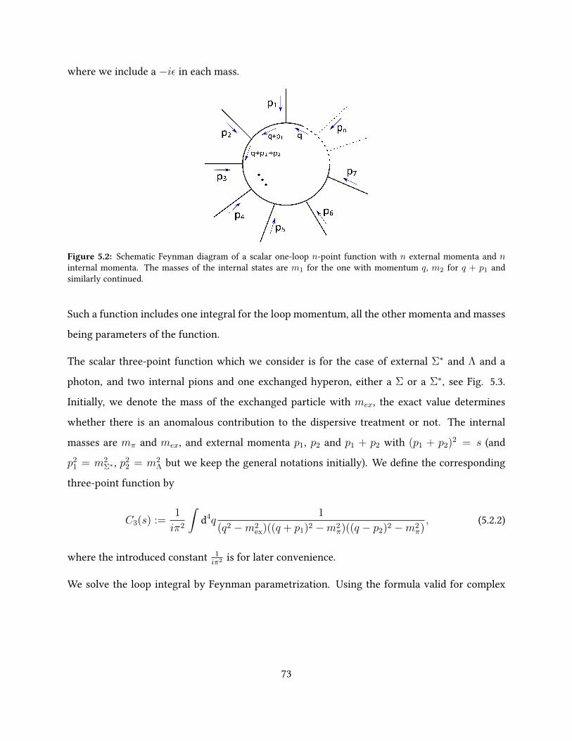
where we include a −iε in each mass.
Figure 5.2: Schematic Feynman diagram of a scalar one-loop n-point function with n external momenta and ninternal momenta. The masses of the internal states are m1 for the one with momentum q, m2 for q + p1 andsimilarly continued.
Such a function includes one integral for the loop momentum, all the other momenta and masses
being parameters of the function.
The scalar three-point function which we consider is for the case of external Σ∗ and Λ and a
photon, and two internal pions and one exchanged hyperon, either a Σ or a Σ∗, see Fig. 5.3.
Initially, we denote the mass of the exchanged particle with mex, the exact value determines
whether there is an anomalous contribution to the dispersive treatment or not. The internal
masses are mπ and mex, and external momenta p1, p2 and p1 + p2 with (p1 + p2)2 = s (and
p21 = m2
Σ∗ , p22 = m2
Λ but we keep the general notations initially). We dene the corresponding
three-point function by
C3(s) :=1
iπ2
∫d4q
1
(q2 −m2ex)((q + p1)2 −m2
π)((q − p2)2 −m2π), (5.2.2)
where the introduced constant 1iπ2 is for later convenience.
We solve the loop integral by Feynman parametrization. Using the formula valid for complex
73
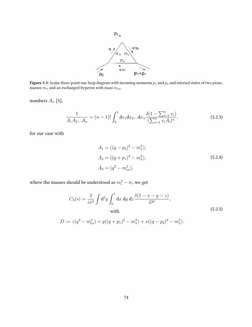
Figure 5.3: Scalar three-point one-loop diagram with incoming momenta p1 and p2 and internal states of two pions,masses mπ and an exchanged hyperon with mass mex.
numbers Ai, [5],
1
A1A2...An= (n− 1)!
∫ 1
0
dx1dx2...dxnδ(1−∑n
i=1 xi)
(∑n
i=1 xiAi)n, (5.2.3)
for our case with
A1 = ((q − p2)2 −m2π),
A2 = ((q + p1)2 −m2π),
A3 = (q2 −m2ex),
(5.2.4)
where the masses should be understood as m2i − iε, we get
C3(s) =2
iπ2
∫d4q
∫ 1
0
dx dy dzδ(1− x− y − z)
D3,
with
D := z(q2 −m2ex) + y((q + p1)2 −m2
π) + x((q − p2)2 −m2π).
(5.2.5)
74
We rst solve the d4q integral, by rewriting
D = (x+ y + z)q2 + 2q(yp1 − xp2)−
− zm2ex − ym2
π − xm2π + yp2
1 + xp22 →
→ (q + yp1 − xp2)2 − (yp1 − xp22)−
− zm2ex − ym2
π − xm2π + yp2
1 + xp22
(5.2.6)
where the arrow indicates the usage of the δ-function in the integral for x, y, z. Shifting variable
to q = q+yp1−xp2 leaves the integral measure unchanged, d4q = d4q, and the limits unchanged,
viz.
C3(s) =2
iπ2
∫ 1
0
dx dy dzδ(1− x− y − z)
∫d4q
1
D3,
with
D =q2 − (yp1 − xp2)2 − zm2ex − ym2
π − xm2π + yp2
1 + xp22 + iε
(5.2.7)
where we have added all the innitesimal imaginary parts of the masses to a new +iε.
One may either proceed using a Wick rotation which takes the integral into Euclidean space, or
one may directly use formulas for d-dimensional integrals for Minkowski space vector l given
for example in [5],
∫ddl
(2π)d1
(l2 −∆)n=
(−1)ni
(4π)d/2Γ(n− d
2)
Γ(n)
(1
∆
)n− d2
. (5.2.8)
We use this formula with
d = 4 , n = 3,
∆ = (yp1 − xp2)2 + zm2ex + ym2
π + xm2π − yp2
1 − xp22 − iε
(5.2.9)
and the denition of the gamma function Γ(n) for n ∈ Z,
Γ(n) = (n− 1)!. (5.2.10)
75
We nally write
C3(s) =2
iπ2
∫ 1
0
dx dy dzδ(1− x− y − z)−i(2π)4
(4π)2
Γ(1)
Γ(3)
(1
∆
)=
= −∫ 1
0
dx dy dzδ(1− x− y − z)
(1
∆
) (5.2.11)
with
∆ = y2p21 − 2xyp1p2 + x2p2
2 + zm2ex + ym2
π + xm2π − yp2
1 − xp22 =
= y(y − 1)p21 + x(x− 1)p2
2 − 2xyp1p2 + zm2ex + ym2
π + xm2π →
→ −(yzp2
1 + xzp22 + xys− zm2
ex − ym2π − xm2
π
),
(5.2.12)
using again the δ-function, which gives nally
C3(s) =
∫ 1
0
dx dy dzδ(1− x− y − z)
(yzp21 + xzp2
2 + xys− zm2ex − ym2
π − xm2π). (5.2.13)
We perform the integral over z which reduces the integral over x and y to a triangle in the plane,
C3(s) =
∫ 1
0
dx∫ 1−x
0
dy1
D1
,
with
D1 = −x2p22 − y2p2
1 + xy(s− p21 − p2
2) + x(p22 +m2
ex −m2π) + y(p2
1 +m2ex −m2
π)−m2ex.
(5.2.14)
a change of variables x = 1− x′ gives
∫ 0
1
(−dx)
∫ x
0
dy =
∫ 1
0
dx∫ x
0
dy. (5.2.15)
This leads us to a form which resembles greatly that given by ’t Hooft and Veltman [25], using
p21 = m2
1, p22 = m2
2,
C3(s) = −∫ 1
0
dx∫ x
0
dy1
(Ax2 +By2 + Cxy +Dx+ Ey + F )(5.2.16)
76
with the Feynman parameters being
A = m22 , B = m2
1 , C = s−m21 −m2
2,
D = m2ex −m2
2 −m2π , E = m2
2 +m2π −m2
ex − s , F = m2π + iε.
(5.2.17)
Now follows a row of manipulations which reduces the expression to one-dimensional integrals
where the integration does not cross any branch cuts.
Let us rst perform a change of variables, y = y′ + τx which gives
C3(s) = −∫ 1
0
dx∫ (1−τ)x
−τxdy
1
(Bτ 2 + Cτ + A)x2 +By2 + (C + 2τB)xy + (D + τE)x+ Ey + F
(5.2.18)
and choose the transformation parameter τ such that it satises
(Bτ 2 + Cτ + A) = 0 (5.2.19)
which takes the integrand in (5.2.18) to the form
f(x, y) :=1
x((C + 2τB)y +D + τE) +By2 + Ey + F ). (5.2.20)
Dividing the y integral into two parts
−C3(s) =
∫ 1
0
dx∫ 0
−τxdyf(x, y) +
∫ 1
0
dx∫ (1−τ)x
0
dyf(x, y), (5.2.21)
for which we portray the integration domain in Fig. (5.4) where we assume 0 < τ < 1 for the
sake of graphics.
We change the order of integration,
−C3(s) =
∫ 1−τ
0
dy∫ 1
−y/(1−τ)
dxf(x, y) +
∫ 0
−τxdy∫ 1
−y/τdxf(x, y), (5.2.22)
77
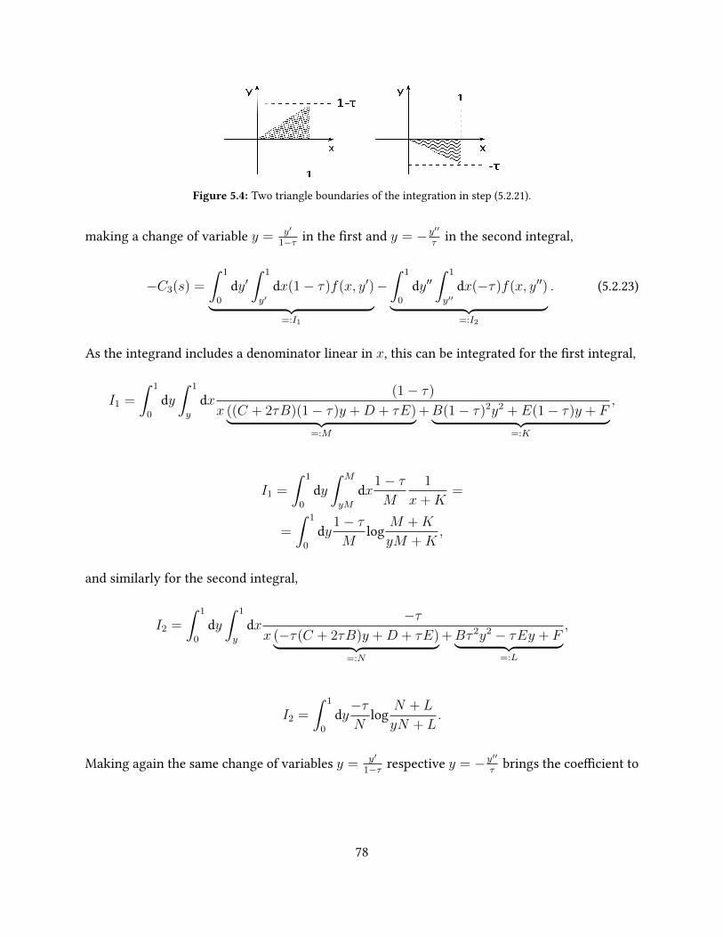
Figure 5.4: Two triangle boundaries of the integration in step (5.2.21).
making a change of variable y = y′
1−τ in the rst and y = −y′′
τin the second integral,
−C3(s) =
∫ 1
0
dy′∫ 1
y′dx(1− τ)f(x, y′)︸ ︷︷ ︸
=:I1
−∫ 1
0
dy′′∫ 1
y′′dx(−τ)f(x, y′′)︸ ︷︷ ︸=:I2
. (5.2.23)
As the integrand includes a denominator linear in x, this can be integrated for the rst integral,
I1 =
∫ 1
0
dy∫ 1
y
dx(1− τ)
x ((C + 2τB)(1− τ)y +D + τE)︸ ︷︷ ︸=:M
+B(1− τ)2y2 + E(1− τ)y + F︸ ︷︷ ︸=:K
,
I1 =
∫ 1
0
dy∫ M
yM
dx1− τM
1
x+K=
=
∫ 1
0
dy1− τM
logM +K
yM +K,
and similarly for the second integral,
I2 =
∫ 1
0
dy∫ 1
y
dx−τ
x (−τ(C + 2τB)y +D + τE)︸ ︷︷ ︸=:N
+Bτ 2y2 − τEy + F︸ ︷︷ ︸=:L
,
I2 =
∫ 1
0
dy−τN
logN + L
yN + L.
Making again the same change of variables y = y′
1−τ respective y = −y′′
τbrings the coecient to
78
the same form in both integrals,
−C3(s) =
∫ 1−τ
0
dy1
Plog
P +By2 + Ey + F
(y P1−τ ) +By2 + Ey + F
−
−∫ −τ
0
dy1
Plog
P +By2 + Ey + F
−y Pτ
+By2 + Ey + F,
P :=(C + 2τB)y +D + τE.
(5.2.24)
Dividing the logarithm into a sum of logarithms and fusing the integration for the numerator in
the logarithm, we get three integrals,
−C3(s) =
∫ 1−τ
−τdy
1
Plog(P +By2 + Ey + F
)−
−∫ 1−τ
0
dy1
Plog(By2 + Ey + F + y
P
1− τ
)+
+
∫ −τ0
dy1
Plog(By2 + Ey + F − yP
τ
).
(5.2.25)
There is a pole in the integrand when P = 0. If the numerator does not also vanish at this
point, then the residue of the integral in the complex plane does not vanish. We notice that the
integration boundaries in the three integrals sum up to zero for a constant term, so we may add
a term independent of y in all integrals without changing the value. If this term is chosen such
that it matches the rst logarithm argument for the point when P = 0, then also the numerator
is zero, giving a zero residue. We note that at P = 0, all arguments of the logarithms are the
same, By2 + Ey + F . Let y0 be the point P (y0) = 0, then
−C3(s) =
∫ 1−τ
−τdy
1
P
(log(P +By2 + Ey + F
)− log
(By2
0 + Ey0 + F))−
−∫ 1−τ
0
dy1
P
(log(By2 + Ey + F + y
P
1− τ
)− log
(By2
0 + Ey0 + F))
+
+
∫ −τ0
dy1
P
(log(By2 + Ey + F − yP
τ
)− log
(By2
0 + Ey0 + F))
,
(5.2.26)
79
where the value of y0 is
y0 = − D + τE
C + 2τB. (5.2.27)
Using the values of the Feynman parameters given in (5.2.17) this can be directly evaluated for
cases when τ is real. For τ ∈ C, the integration boundaries are ill-dened in the complex plane.
We therefore perform one additional change of variables which yields the most general result as
given also in [25], which we will use in the calculations.
Changing variables in each integral accordingly: y = y′ − τ , y = (1− τ)y′′ and y = −τy′′′,
−C3(s) =
∫ 1
0
dy1
(C + 2τB) +D + τE(log(By2 + (E + C)y + A+D + F )− log(By2
0 + Ey0 + F ))−
−∫ 1
0
dy1− τ
(C + 2τB)(1− τ)y +D + τE(log((A+B + C)y2 + (E +D)y + F )− log(By2
0 + Ey0 + F ))
+
+
∫ 1
0
dy−τ
−(C + 2τB)τy +D + τE(log(Ay2 +Dy + F )− log(By2
0 + Ey0 + F ))
(5.2.28)
which is the nal result for the loop calculation and is also valid for complex values of τ . This may
be further rewritten in terms of di-logarithms [25, 31] or Appell functions [32] but in this work
we use (5.2.28) for our direct loop calculations which we compare to the dispersive calculations.
5.3 Analytic properties along the unitarity cut
In this section we rst examine the discontinuity of the scalar triangle diagram along the unitarity
cut. We present a step by step derivation to obtain the unitarity discontinuity. We then examine
the Riemann sheets for the unitarity cut, which will be essential when studying the trajectories
of the branch points of the discontinuity later in Section 5.4.
80
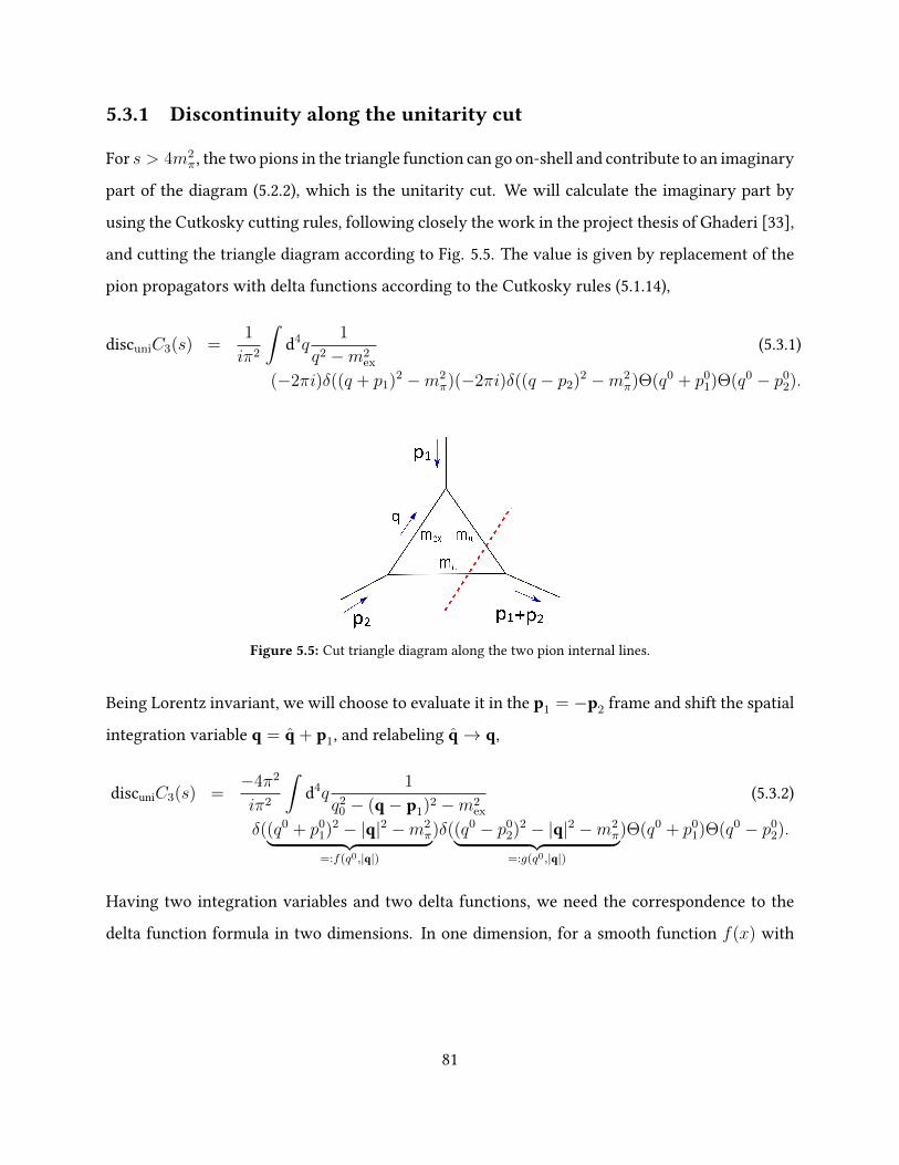
5.3.1 Discontinuity along the unitarity cut
For s > 4m2π, the two pions in the triangle function can go on-shell and contribute to an imaginary
part of the diagram (5.2.2), which is the unitarity cut. We will calculate the imaginary part by
using the Cutkosky cutting rules, following closely the work in the project thesis of Ghaderi [33],
and cutting the triangle diagram according to Fig. 5.5. The value is given by replacement of the
pion propagators with delta functions according to the Cutkosky rules (5.1.14),
discuniC3(s) =1
iπ2
∫d4q
1
q2 −m2ex
(5.3.1)
(−2πi)δ((q + p1)2 −m2π)(−2πi)δ((q − p2)2 −m2
π)Θ(q0 + p01)Θ(q0 − p0
2).
Figure 5.5: Cut triangle diagram along the two pion internal lines.
Being Lorentz invariant, we will choose to evaluate it in the p1 = −p2 frame and shift the spatial
integration variable q = q + p1, and relabeling q→ q,
discuniC3(s) =−4π2
iπ2
∫d4q
1
q20 − (q− p1)2 −m2
ex
(5.3.2)
δ((q0 + p01)2 − |q|2 −m2
π︸ ︷︷ ︸=:f(q0,|q|)
)δ((q0 − p02)2 − |q|2 −m2
π︸ ︷︷ ︸=:g(q0,|q|)
)Θ(q0 + p01)Θ(q0 − p0
2).
Having two integration variables and two delta functions, we need the correspondence to the
delta function formula in two dimensions. In one dimension, for a smooth function f(x) with
81
zeros xi, we write
δ(f(x)) =∑xi
δ(x− xi)|f ′(xi)|
. (5.3.3)
For two smooth functions f(x, y) and g(x, y), with a common zero (x0, y0) in the interval of
integration, we use the formula given in [33],
δ(f(x, y))δ(g(x, y)) =δ(x− x0)δ(y − y0)∣∣∣∣ ∂f∂x ∂g∂y ∣∣∣
(x0,y0)− ∂f
∂y∂g∂x
∣∣∣(x0,y0)
∣∣∣∣ . (5.3.4)
The zero point (q0∗, |q|∗) which obeys the Θ-function of the function f(q0, |q|) is
q0∗ = −p0
1 +√|q|2 +m2
π, (5.3.5)
we use the g(q0, |q|) to obtain the value of |q| for which this is simultaneously a zero of both
functions,
(q0∗ − p0
2)2 − |q|2∗ −m2π
!= 0,
→ |q|∗ =
√s
2
√1− 4m2
π
s.
(5.3.6)
The partial derivatives of the function evaluated at the zero point are,
∂f
∂q0=√s ,
∂f
∂|q| = −2|q|∗∂g
∂q0= −√s ,
∂g
∂|q| = −2|q|∗(5.3.7)
giving ∣∣∣∣∣ ∂f∂q0
∂g
∂|q|
∣∣∣∣(q0∗,|q|∗)
− ∂f
∂|q|∂g
∂q0
∣∣∣∣(q0∗,|q|∗)
∣∣∣∣∣ = 4√s|q|∗. (5.3.8)
82
Using all this reduces the discontinuity to
discuniC3(s) =i√s|q|∗
∫d4q
1
q20 − (q− p1)2 −m2
ex
δ(q0 − q0∗)δ(|q| − |q|∗) =
=i√s|q|∗
∫|q|2d|q|dΩ
1
(q0∗)
2 − (q− p1)2 −m2ex
δ(|q| − |q|∗) =
=2πi|q|2∗√s|q|∗
∫ 1
−1
d cos(θ)1
(q0∗)
2 − |q|2∗ + 2|q|∗|p1| cos θ − |p1|2 −m2ex
.
(5.3.9)
Without loss of generality, we may choose the polar angle θ of the vector q to be the angle
between q and p1. Denoting z := cos θ,
discuniC3(s) =−4πi|q|∗√
s
∫ 1
−1
dz1
a(s)− b(s)z ,
a(s) := 2|q|2∗ + 2p21 + 2(q0
∗)2 + 2m2
ex,
b(s) := 4|q|∗|p1|
(5.3.10)
which solves to
discuniC3(s) =−4πi|q|∗√
s
1
b(s)log
a(s) + b(s)
a(s)− b(s) . (5.3.11)
Using the center of momentum value of |p1| =
√λ(s,m2
1,m22)
2√s
, and (5.3.7) and after some simpli-
cations,
discuniC3(s) =−2πi√
λ(s,m21,m
22)
loga(s) + b(s)
a(s)− b(s)Θ(s− 4m2π), (5.3.12)
including now the Θ-function explicitly to denote that this occurs only if the two pions can go
on-shell. The imaginary part arising from the unitarity cut only of the three-point function is
83
then
ImuniC3(s) = −π 1√λ(s,m2
1,m22)
loga(s) + b(s)
a(s)− b(s)Θ(s− 4m2π)
with
a(s) = s+ 2m2ex −m2
1 −m22 − 2m2
π,
b(s) =√λ(s,m2
1,m22)
√1− 4m2
π
s.
(5.3.13)
The Θ-function denes a discontinuity with a corresponding Riemann surface. The logarithm
in the discontinuity in turn has branch points which may or may not lie on the rst Riemann
sheet of the unitarity discontinuity. The dispersive integral includes all of the complex plane on
one Riemann sheet. If the branch point is thus on a dierent Riemann sheet, the anomalous cut
associated with the branch point will not contribute to the dispersive integral.
The unitarity discontinuity appears in the unitarity integral for the dispersion relation in the
three-point function, and will be discussed more in Section 5.4. Evaluated on the real axis, the
logarithm has dierent denitions on dierent intervals. This is in order to ensure that it is a
smooth function. We introduce points on the real line for which the sign of the argument of the
logarithm in (5.3.13) changes,
s1 := (mΣ∗ −mΛ)2,
s2 := scr,
s3 := (mΣ∗ +mΛ)2,
(5.3.14)
with a(scr) = 0, scr = m21 + m2
2 + 2m2π − 2m2
ex. The denition of the logarithm on the real axis
84
is then
discuniC3(s) = 2i
− 2πσ(s)
b(s)
(tan−1
( |b(s)|a(s)
+ π
)), s1 < s ≤ s2,
− 2πσ(s)
b(s)
(tan−1
( |b(s)|a(s)
)), s2 < s ≤ s3,
− πσ(s)
b(s)
(log(a(s) + b(s)
a(s)− b(s)
)), s3 < s.
(5.3.15)
which is the expression we use in the calculations of the unitarity integral for the scalar triangle
diagram.
5.3.2 Riemann sheets of the unitarity cut
We consider here the Riemann surface of the unitarity cut. The discontinuity along this cut is
given in (5.3.12) (omitting the Θ-function),
discuniC3(s) = −2πiσ(s)
b(s)log
a(s) + b(s)
a(s)− b(s) = −2πiσ(s)f(s),
σ(s) :=
√1− 4m2
π
s,
f(s) :=1
b(s)log
a(s) + b(s)
a(s)− b(s) .
(5.3.16)
We see that f(s) has no pole when b(s) = 0, as, expanding the logarithm around b(s)a(s)→ 0 gives
f(s) =1
b(s)log
1 + b(s)a(s)
1− b(s)a(s)
=
=1
b(s)
(0 + 2
b(s)
a(s)+
1
3!4
(b(s)
a(s)
)3
+O
(b(s)
a(s)
)5)
=
= 21
a(s)+O
(b(s)2
).
(5.3.17)
At threshold s = 4m2π, for which b(s) = 0, f(s) is continuous. The logarithm in f(s) is contin-
uous (complex-valued) everywhere around the unitarity cut. If it is analytic in a domain around
85
the unitarity cut, we may analytically continue it to the entire complex plane and further for s
on the unitarity cut,
f(s) = f(s+ iε) = f(s− iε) , for ε→ 0. (5.3.18)
Notice that the above equation holds only for the case when only the unitarity cut is present. If
additional cuts arise in the rst Riemann sheet, the above no longer holds. The core of the present
work is the examination of which cases there is an additional cut and how we implement it in
the calculations with dispersion relations.
The discontinuity ofC3(s) at the unitarity cut is still aected by the σ(s) factor. As it stands, σ(s)
has a cut on the line segment s ∈ [0, 4m2π), but it is continuous on the unitarity cut [4m2
π,∞).
Let us dene a function which has a cut on the unitarity cut, along the same line of procedure as
done by Moussallam [34] and also discussed in [3],
σ0(s) : =
√4m2
π
s− 1,
σ0(s) = iσ(s) , s ∈ C.(5.3.19)
On an open domain around the unitarity cut, σ(s) is continuous and for ε→ 0,
σ(s+ iε) = σ(s) , for s ∈ [4m2π,∞), (5.3.20)
for s on the unitarity cut we evaluate
σ(s+ iε) = iσ0(s+ iε), (5.3.21)
which we write by using (5.3.20) as
σ0(s+ iε) = −iσ(s). (5.3.22)
86
Using the denition of the functions, we can show that
σ(s− iε) = (σ(s+ iε))∗ = (iσ0(s+ iε))∗ =
= −i(σ0(s+ iε))∗ = −iσ0(s− iε),(5.3.23)
which shows the Schwarz’s reection principle is obeyed by these functions. Using continuity of
σ(s) and σ(s) ∈ R for s ∈ R,
σ0(s− iε) = iσ(s). (5.3.24)
Now we dene the three-point function on a Riemann sheet, denoted by C13(s) and one on the
next sheet as C23(s) which we demand should be an analytic continuation through the unitarity
cut s ∈ [4m2π,∞),
C23(s+ iε)
!= C1
3(s− iε). (5.3.25)
By denition of the discontinuity on the rst Riemann sheet from (5.3.16),
C13(s+ iε)− C1
3(s− iε) = discuniC3(s). (5.3.26)
We rewrite this as
C23(s+ iε) = C1
3(s+ iε) + 2πiσ(s)f(s) (5.3.27)
but on the unitarity cut, f(s) is continuous, f(s) = f(s+ iε) and we may use (5.3.22) to relate
C23(s+ iε) = C1
3(s+ iε)− 2πσ0(s+ iε)f(s+ iε) (5.3.28)
which can be generalized by analytic continuation for any complex s ∈ C, and so we may evaluate
87
it at s− iε,
C23(s− iε) = C1
3(s− iε)− 2πσ0(s− iε)f(s− iε). (5.3.29)
Again using continuity of f(s) at the unitarity cut and (5.3.24),
C23(s− iε) = C1
3(s− iε)− 2πiσ(s)f(s) = C13(s+ iε). (5.3.30)
Hence, the rst Riemann sheet is the analytic continuation of the second one, C13(s− iε) = C2
3(s+ iε)
C23(s− iε) = C1
3(s+ iε),(5.3.31)
which precisely is the condition for only two Riemann sheets. As a consequence, any point
crossing the unitarity cut from one sheet to the other will have crossed all the Riemann sheets of
the unitarity cut.
5.4 Dispersive calculations
In this section we will consider the branch points of the logarithm in the discontinuity and exam-
ine their trajectories in the complex plane. Depending on their location, the dispersive integral
will or will not need an anomalous contribution. This is demonstrated by calculation for various
masses and comparison to the direct calculation.
5.4.1 Branch points of the discontinuity
A cut arises in the unitarity discontinuity at the stage of the integral (5.3.10), where the denomi-
nator of the integrand runs over poles when a(s) = b(s)z, in the interval z ∈ [−1, 1]. We examine
the location of these points on the cut by working in z2, which is in the interval [0, 1], and the
88
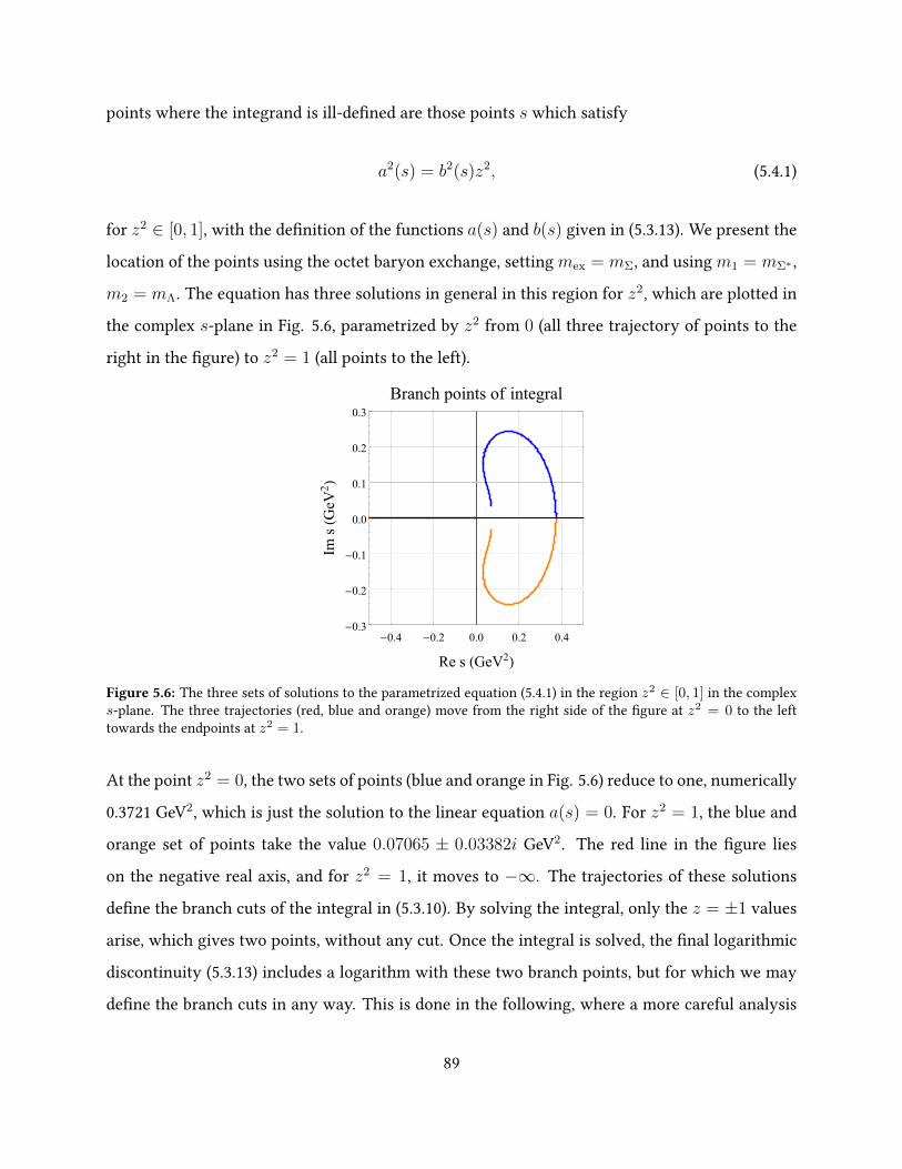
points where the integrand is ill-dened are those points s which satisfy
a2(s) = b2(s)z2, (5.4.1)
for z2 ∈ [0, 1], with the denition of the functions a(s) and b(s) given in (5.3.13). We present the
location of the points using the octet baryon exchange, setting mex = mΣ, and using m1 = mΣ∗ ,
m2 = mΛ. The equation has three solutions in general in this region for z2, which are plotted in
the complex s-plane in Fig. 5.6, parametrized by z2 from 0 (all three trajectory of points to the
right in the gure) to z2 = 1 (all points to the left).
-0.4 -0.2 0.0 0.2 0.4-0.3
-0.2
-0.1
0.0
0.1
0.2
0.3
Re s (GeV2)
Ims(GeV
2)
Branch points of integral
Figure 5.6: The three sets of solutions to the parametrized equation (5.4.1) in the region z2 ∈ [0, 1] in the complexs-plane. The three trajectories (red, blue and orange) move from the right side of the gure at z2 = 0 to the lefttowards the endpoints at z2 = 1.
At the point z2 = 0, the two sets of points (blue and orange in Fig. 5.6) reduce to one, numerically
0.3721 GeV2, which is just the solution to the linear equation a(s) = 0. For z2 = 1, the blue and
orange set of points take the value 0.07065 ± 0.03382i GeV2. The red line in the gure lies
on the negative real axis, and for z2 = 1, it moves to −∞. The trajectories of these solutions
dene the branch cuts of the integral in (5.3.10). By solving the integral, only the z = ±1 values
arise, which gives two points, without any cut. Once the integral is solved, the nal logarithmic
discontinuity (5.3.13) includes a logarithm with these two branch points, but for which we may
dene the branch cuts in any way. This is done in the following, where a more careful analysis
89
of the two branch points is performed, but with the logarithm as a starting point.
The branch points of the logarithm in the unitarity discontinuity are observed by writing out the
logarithm part explicitly,
log(a(s) + b(s)
a(s)− b(s)
)= log(a(s) + b(s))− log(a(s)− b(s)), (5.4.2)
for regions when the imaginary part of the numerator and denominator are the same. The branch
points of the logarithm are the points where one argument of the logarithms vanishes (corre-
sponding to z2 = 1 in (5.4.1)),
a(s) = b(s)
a(s) = −b(s)
a2(s) = b2(s), (5.4.3)
being a third-order equation in which the highest order term vanishes, it gives us two solutions
s± to the equation
As2 +Bs+ C = 0 (5.4.4)
with
A := 2(2m2ex −m2
1 −m22 − 2m2
π) + 2(m21 +m2
2) + 4m2π,
B := (2m2ex −m2
1 −m22 − 2m2
π)2 − (m21 +m2
2)2 − 2(m21 +m2
2)4m2π,
C := 4m2π(m2
1 +m22)2.
(5.4.5)
Working out the algebra gives
s± =1
2(m2
1 +m22 + 2m2
π −m2ex)+
+m2π(m2
1 +m22)−m4
π −m11m
22
2m2ex
±√λ(m2
1,m2ex,m
2π)λ(m2
2,m2ex,m
2π))
2m2ex
.
(5.4.6)
The location of the branch point depends on the internal and external masses. In the following
90
we will consider dierent cases which demonstrates the location of the branch points on the two
Riemann sheets of the unitarity cut. This approach of tracking the branch point in the complex
plane is also performed by Lucha et al. [35] and corresponding erratum [36].
The unitarity discontinuity (5.3.12) is of the form [3]
r(s)log p(s) (5.4.7)
with a function r(s) which has poles, but is continuous over the branch cut of the logarithm. The
discontinuity of the total function is then i2πr(s). This yields then that the discontinuity of the
unitarity discontinuity, which is then the anomalous discontinuity of the three-point function, is
discanomC3(s) =4π2√
λ(s,m21,m
22)
(5.4.8)
along the anomalous branch cut. We may dene this branch cut in any way. In general, the
branch point will be complex and the branch cut is then located not merely on the real axis. With
respect to the Riemann sheets of the unitarity cut, the branch points may either be on the rst
or the second Riemann sheet. If the location is on the second Riemann sheet, we may dene the
branch cut in such a way that it never intersects the unitarity cut. If any branch point lies on
the rst Riemann sheet, the discontinuity along the entire branch cut must be considered. By
dening it in a way that it intersects the unitarity cut, the part of the cut on the other side of
the unitarity cut crosses over to the second Riemann sheet and does then not contribute to the
dispersion relation. In this way we can reduce the integral over the branch cut to a nite line
segment connecting the branch point and the unitarity cut. In addition, we may dene the point
of connection to be the threshold of the unitarity cut, in which case the discontinuities are along
two lines smoothly connected.
As we know from the spectral theorem (5.1.4), the discontinuity is related to the imaginary part
of an analytic function. For amplitudes only with a unitarity cut with the Θ(s− 4m2π) function,
the amplitude is purely real below the threshold. The additional anomalous discontinuity which
91
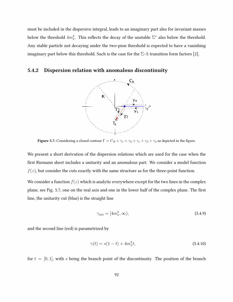
must be included in the dispersive integral, leads to an imaginary part also for invariant masses
below the threshold 4m2π. This reects the decay of the unstable Σ∗ also below the threshold.
Any stable particle not decaying under the two-pion threshold is expected to have a vanishing
imaginary part below this threshold. Such is the case for the Σ-Λ transition form factors [2].
5.4.2 Dispersion relation with anomalous discontinuity
Figure 5.7: Considering a closed contour Γ = CR + γ1 + γ2 + γε + γ3 + γ4 as depicted in the gure.
We present a short derivation of the dispersion relations which are used for the case when the
rst Riemann sheet includes a unitarity and an anomalous part. We consider a model function
f(z), but consider the cuts exactly with the same structure as for the three-point function.
We consider a function f(z) which is analytic everywhere except for the two lines in the complex
plane, see Fig. 5.7, one on the real axis and one in the lower half of the complex plane. The rst
line, the unitarity cut (blue) is the straight line
γuni = [4m2π,∞), (5.4.9)
and the second line (red) is parametrized by
γ(t) = s(1− t) + 4m2πt, (5.4.10)
for t = [0, 1], with s being the branch point of the discontinuity. The position of the branch
92
point is further examined in Sections 5.4.3 and 5.4.4. For the sake of this section, the anomalous
discontinuity γ(t) is a denition only.
Taking a closed contour Γ = CR+γ1 +γ2 +γε+γ3 +γ4, as depicted in Fig. (5.7), closes a domain
in the complex z plane, such that on the interior Int(Γ) of the closed contour, the function f(z) is
analytic. The CR represents a circular arch with radiusRwith a segment with length ε′ removed.
By the Cauchy integral formula [26], the value of the function at any point z ∈ Int(Γ), is given
by
f(z) =1
2πi
∮Γ
dz′f(z′)
z′ − z . (5.4.11)
Writing it as a sum of integrals along the line segments,
f(z) =1
2πi
(∫CR
+
∫γ1
+
∫γ2
+
∫γε
+
∫γ3
+
∫γ4
)dz′
f(z′)
z′ − z . (5.4.12)
By letting ε→ 0, the contour γε reduces to a point, and
∫γε
→ 0. (5.4.13)
On the circular arch, the integral may be related to an upper boundary,∣∣∣∣∫CR
dz′f(z′)
z′ − z
∣∣∣∣ ≤ maxz′∈CR
∣∣∣∣ f(z′)
z′ − z
∣∣∣∣ l(CR), (5.4.14)
where the length of the arch l(CR) goes to 2πR as ε′ → 0. By the inverse triangle inequality [26]
we have
1
|z′ − z| ≤1
R + |z| , (5.4.15)
which takes (5.4.14) to the form∣∣∣∣∫CR
dz′f(z′)
z′ − z
∣∣∣∣ ≤ 1
R + |z| maxz′∈CR
|f(z′)|. (5.4.16)
93
If we require the function to be such that it vanishes at complex innity, |f(z)| → 0 as |z| → ∞,
then the integral over the circular arch vanishes,
limR→∞
∫CR
dz′f(z′)
z′ − z = 0. (5.4.17)
As ε→ 0, the integrals along the straight line segments γ2 and γ3 become the integrals along the
parametrized curve γ(t), however in dierent directions and with the function evaluated at the
left and right side of the segment respectively,
limε→0
∫γ2
dz′f(z′)
z′ − z = −∫γ
dγdt
dtf−(γ(t))
γ(t)− z ,
limε→0
∫γ3
dz′f(z′)
z′ − z =
∫γ
dγdt
dtf+(γ(t))
γ(t)− z ,(5.4.18)
and the sum of the two integrals,
limε→0
(∫γ2
+
∫γ3
)=
∫γ
dtdγdtf+(γ(t))− f−(γ(t))
γ(t)− z =
∫γ
dtdγdt
discanomf(γ(t))
γ(t)− z , (5.4.19)
with the anomalous discontinuity discanom along the cut γ(t).
In the same way, we deduce the sum of the integrals along the line segments above and below
the unitarity cut,
limε→0
(∫γ1
+
∫γ4
)=
∫γ
dtdγdtf+(γuni)− f−(γuni)
γuni − z=
∫γ
dtdγdt
discunif(γuni)
γuni − z. (5.4.20)
Being a line segment along the real axis, the integral over γuni is rewritten in a more compact
form:
∫γ
dtdγdt
discunif(γuni)
γuni − z=
∫ ∞4m2
π
dz′discunif(z′)
z′ − z . (5.4.21)
For functions with discontinuities, the function value on the real axis is dened as the limit of
94
the complex value evaluated in the upper complex half plane:
f(z) = limε→0
f(z + iε) for z ∈ R, (5.4.22)
and so we may set the argument z to z + iε in order to avoid singularities in the integral,
∫γ
dtdγdt
discunif(γuni)
γuni − z=
∫ ∞4m2
π
dz′discunif(z′)
z′ − z − iε . (5.4.23)
The Cauchy integral formula for f(z) in (5.4.12) nally becomes
f(z) =1
2πi
(∫γ
dtdγdt
discanomf(γ(t))
γ(t)− z +
∫ ∞4m2
π
dz′discunif(z′)
z′ − z − iε .), (5.4.24)
which is the form of the unsubtracted dispersion relation which is used for the scalar three-point
function in Section 5.4.4 with an anomalous contribution.
5.4.3 Decuplet exchange,mex = mΣ∗
In the case of the exchanged particle being the decuplet Σ∗ in the scalar triangle diagram (along
with the two-pion exchange), we do not expect an anomalous threshold as the mass condition
(5.1.23) is not fullled. We denote the three-point function with an Σ∗ exchange with CΣ∗3 (s).
Now we examine this three-point function by calculating it with the aid of dispersion relations
for the case of only a unitarity contribution and with the anomalous contributions and comparing
it to the direct calculation. Without the anomalous cut, the only contribution to the dispersion
relation comes from the unitarity cut,
CΣ∗
3 (s)?=
1
2πi
∫ ∞4m2
π
ds′discuniC
Σ∗3 (s′)
s′ − s− iε , (5.4.25)
where we wish to now examine to which extent this equality is satised.
For the anomalous contribution in this case, we examine the branch points of the logarithm in
the unitarity discontinuity. We are at the end interested in the position of the branch points for
95
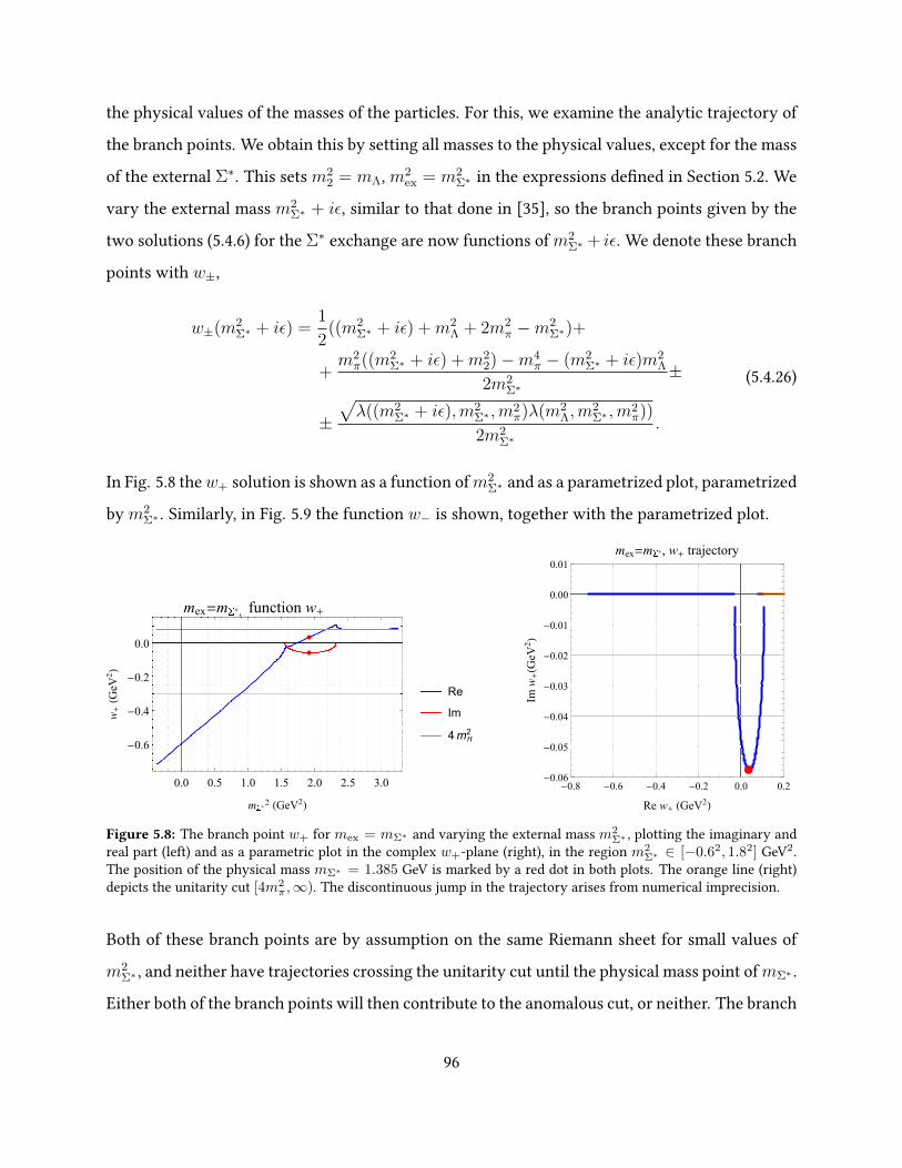
the physical values of the masses of the particles. For this, we examine the analytic trajectory of
the branch points. We obtain this by setting all masses to the physical values, except for the mass
of the external Σ∗. This sets m22 = mΛ, m2
ex = m2Σ∗ in the expressions dened in Section 5.2. We
vary the external mass m2Σ∗ + iε, similar to that done in [35], so the branch points given by the
two solutions (5.4.6) for the Σ∗ exchange are now functions of m2Σ∗ + iε. We denote these branch
points with w±,
w±(m2Σ∗ + iε) =
1
2((m2
Σ∗ + iε) +m2Λ + 2m2
π −m2Σ∗)+
+m2π((m2
Σ∗ + iε) +m22)−m4
π − (m2Σ∗ + iε)m2
Λ
2m2Σ∗
±
±√λ((m2
Σ∗ + iε),m2Σ∗ ,m
2π)λ(m2
Λ,m2Σ∗ ,m
2π))
2m2Σ∗
.
(5.4.26)
In Fig. 5.8 thew+ solution is shown as a function ofm2Σ∗ and as a parametrized plot, parametrized
by m2Σ∗ . Similarly, in Fig. 5.9 the function w− is shown, together with the parametrized plot.
0.0 0.5 1.0 1.5 2.0 2.5 3.0
-0.6
-0.4
-0.2
0.0
m*2 (GeV2)
w+(GeV2)
Re
Im
4mπ2
mex=m*, function w+
-0.8 -0.6 -0.4 -0.2 0.0 0.2-0.06
-0.05
-0.04
-0.03
-0.02
-0.01
0.00
0.01
Re w+ (GeV2)
Imw+(GeV
2)
mex=m *, w+ trajectory
Figure 5.8: The branch point w+ for mex = mΣ∗ and varying the external mass m2Σ∗ , plotting the imaginary and
real part (left) and as a parametric plot in the complex w+-plane (right), in the region m2Σ∗ ∈ [−0.62, 1.82] GeV2.
The position of the physical mass mΣ∗ = 1.385 GeV is marked by a red dot in both plots. The orange line (right)depicts the unitarity cut [4m2
π,∞). The discontinuous jump in the trajectory arises from numerical imprecision.
Both of these branch points are by assumption on the same Riemann sheet for small values of
m2Σ∗ , and neither have trajectories crossing the unitarity cut until the physical mass point ofmΣ∗ .
Either both of the branch points will then contribute to the anomalous cut, or neither. The branch
96
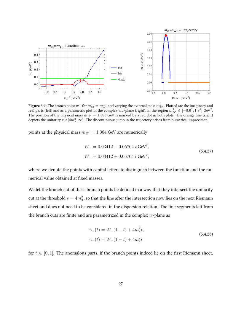
0.0 0.5 1.0 1.5 2.0 2.5 3.0
0.0
0.1
0.2
0.3
0.4
mΣ*2 (GeV2)
w-(GeV2)
Re
Im
4mπ2
mex=mΣ*, function w-
-0.2 0.0 0.2 0.4 0.6 0.8-0.01
0.00
0.01
0.02
0.03
0.04
0.05
0.06
Re w- (GeV2)
Imw-(GeV
2)
mex=m *, w- trajectory
Figure 5.9: The branch pointw− formex = mΣ∗ and varying the external massm2Σ∗ . Plotted are the imaginary and
real parts (left) and as a parametric plot in the complex w−-plane (right), in the region m2Σ∗ ∈ [−0.62, 1.82] GeV2.
The position of the physical mass mΣ∗ = 1.385 GeV is marked by a red dot in both plots. The orange line (right)depicts the unitarity cut [4m2
π,∞). The discontinuous jump in the trajectory arises from numerical imprecision.
points at the physical mass mΣ∗ = 1.384 GeV are numerically
W+ = 0.03412− 0.05764 i GeV2,
W− = 0.03412 + 0.05764 i GeV2,(5.4.27)
where we denote the points with capital letters to distinguish between the function and the nu-
merical value obtained at xed masses.
We let the branch cut of these branch points be dened in a way that they intersect the unitarity
cut at the threshold s = 4m2π, so that the line after the intersection now lies on the next Riemann
sheet and does not need to be considered in the dispersion relation. The line segments left from
the branch cuts are nite and are parametrized in the complex w-plane as
γ+(t) = W+(1− t) + 4m2πt,
γ−(t) = W−(1− t) + 4m2πt
(5.4.28)
for t ∈ [0, 1]. The anomalous parts, if the branch points indeed lie on the rst Riemann sheet,
97
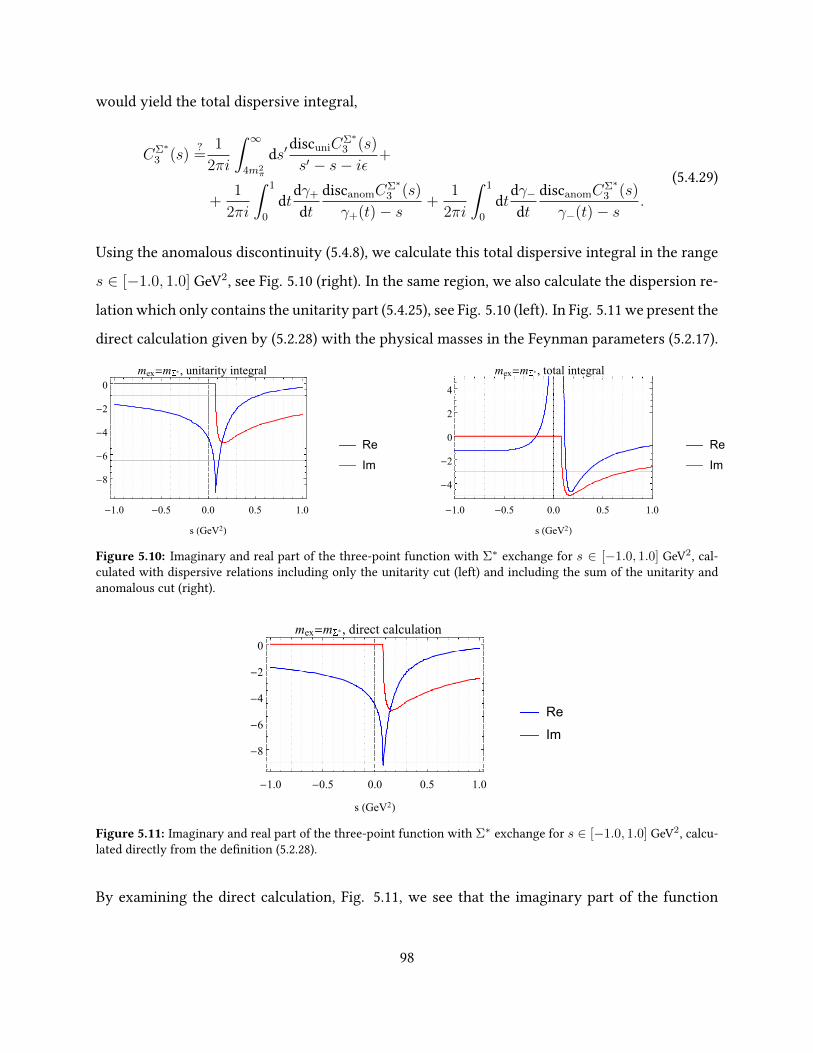
would yield the total dispersive integral,
CΣ∗
3 (s)?=
1
2πi
∫ ∞4m2
π
ds′discuniC
Σ∗3 (s)
s′ − s− iε +
+1
2πi
∫ 1
0
dtdγ+
dtdiscanomC
Σ∗3 (s)
γ+(t)− s +1
2πi
∫ 1
0
dtdγ−dt
discanomCΣ∗3 (s)
γ−(t)− s .
(5.4.29)
Using the anomalous discontinuity (5.4.8), we calculate this total dispersive integral in the range
s ∈ [−1.0, 1.0] GeV2, see Fig. 5.10 (right). In the same region, we also calculate the dispersion re-
lation which only contains the unitarity part (5.4.25), see Fig. 5.10 (left). In Fig. 5.11 we present the
direct calculation given by (5.2.28) with the physical masses in the Feynman parameters (5.2.17).
-1.0 -0.5 0.0 0.5 1.0
-8
-6
-4
-2
0
s (GeV2)
Re
Im
mex=m*, unitarity integral
-1.0 -0.5 0.0 0.5 1.0
-4
-2
0
2
4
s (GeV2)
Re
Im
mex=m*, total integral
Figure 5.10: Imaginary and real part of the three-point function with Σ∗ exchange for s ∈ [−1.0, 1.0] GeV2, cal-culated with dispersive relations including only the unitarity cut (left) and including the sum of the unitarity andanomalous cut (right).
-1.0 -0.5 0.0 0.5 1.0
-8
-6
-4
-2
0
s (GeV2)
Re
Im
mex=m*, direct calculation
Figure 5.11: Imaginary and real part of the three-point function with Σ∗ exchange for s ∈ [−1.0, 1.0] GeV2, calcu-lated directly from the denition (5.2.28).
By examining the direct calculation, Fig. 5.11, we see that the imaginary part of the function
98
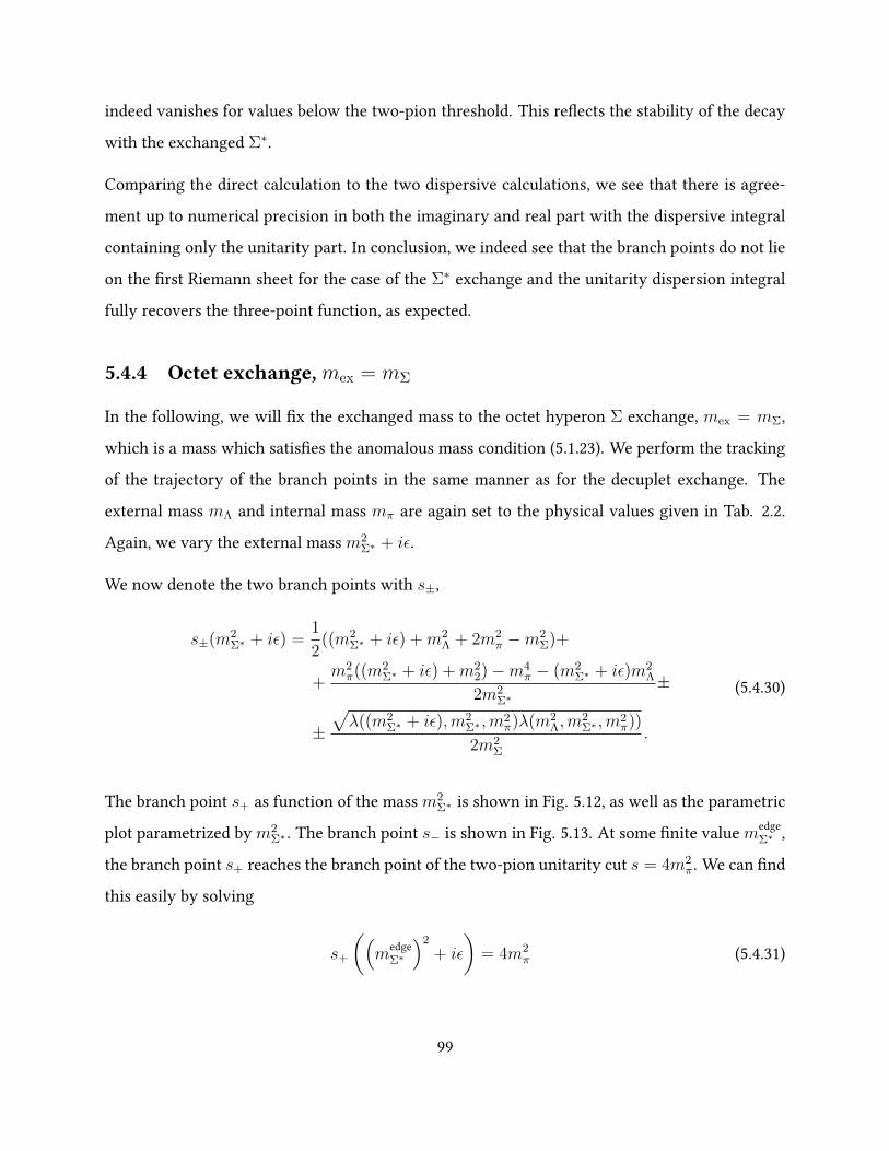
indeed vanishes for values below the two-pion threshold. This reects the stability of the decay
with the exchanged Σ∗.
Comparing the direct calculation to the two dispersive calculations, we see that there is agree-
ment up to numerical precision in both the imaginary and real part with the dispersive integral
containing only the unitarity part. In conclusion, we indeed see that the branch points do not lie
on the rst Riemann sheet for the case of the Σ∗ exchange and the unitarity dispersion integral
fully recovers the three-point function, as expected.
5.4.4 Octet exchange,mex = mΣ
In the following, we will x the exchanged mass to the octet hyperon Σ exchange, mex = mΣ,
which is a mass which satises the anomalous mass condition (5.1.23). We perform the tracking
of the trajectory of the branch points in the same manner as for the decuplet exchange. The
external mass mΛ and internal mass mπ are again set to the physical values given in Tab. 2.2.
Again, we vary the external mass m2Σ∗ + iε.
We now denote the two branch points with s±,
s±(m2Σ∗ + iε) =
1
2((m2
Σ∗ + iε) +m2Λ + 2m2
π −m2Σ)+
+m2π((m2
Σ∗ + iε) +m22)−m4
π − (m2Σ∗ + iε)m2
Λ
2m2Σ∗
±
±√λ((m2
Σ∗ + iε),m2Σ∗ ,m
2π)λ(m2
Λ,m2Σ∗ ,m
2π))
2m2Σ
.
(5.4.30)
The branch point s+ as function of the mass m2Σ∗ is shown in Fig. 5.12, as well as the parametric
plot parametrized by m2Σ∗ . The branch point s− is shown in Fig. 5.13. At some nite value medge
Σ∗ ,
the branch point s+ reaches the branch point of the two-pion unitarity cut s = 4m2π. We can nd
this easily by solving
s+
((m
edgeΣ∗
)2
+ iε
)= 4m2
π (5.4.31)
99
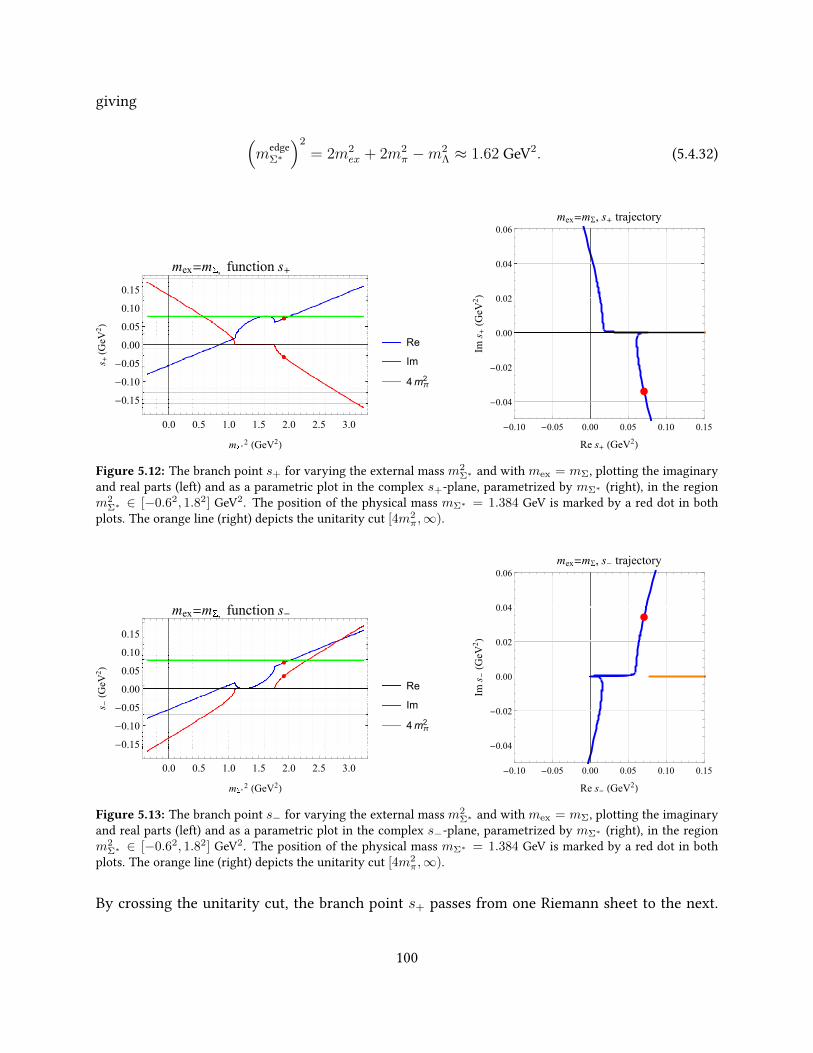
giving
(m
edgeΣ∗
)2
= 2m2ex + 2m2
π −m2Λ ≈ 1.62 GeV2. (5.4.32)
0.0 0.5 1.0 1.5 2.0 2.5 3.0
-0.15
-0.10
-0.05
0.00
0.05
0.10
0.15
m*2 (GeV2)
s+(GeV2)
Re
Im
4mπ2
mex=m, function s+
-0.10 -0.05 0.00 0.05 0.10 0.15
-0.04
-0.02
0.00
0.02
0.04
0.06
Re s+ (GeV2)
Ims+(GeV
2)
mex=mΣ, s+ trajectory
Figure 5.12: The branch point s+ for varying the external mass m2Σ∗ and with mex = mΣ, plotting the imaginary
and real parts (left) and as a parametric plot in the complex s+-plane, parametrized by mΣ∗ (right), in the regionm2
Σ∗ ∈ [−0.62, 1.82] GeV2. The position of the physical mass mΣ∗ = 1.384 GeV is marked by a red dot in bothplots. The orange line (right) depicts the unitarity cut [4m2
π,∞).
0.0 0.5 1.0 1.5 2.0 2.5 3.0
-0.15
-0.10
-0.05
0.00
0.05
0.10
0.15
m*2 (GeV2)
s-(GeV2)
Re
Im
4mπ2
mex=m, function s-
-0.10 -0.05 0.00 0.05 0.10 0.15
-0.04
-0.02
0.00
0.02
0.04
0.06
Re s- (GeV2)
Ims-(GeV
2)
mex=mΣ, s- trajectory
Figure 5.13: The branch point s− for varying the external mass m2Σ∗ and with mex = mΣ, plotting the imaginary
and real parts (left) and as a parametric plot in the complex s−-plane, parametrized by mΣ∗ (right), in the regionm2
Σ∗ ∈ [−0.62, 1.82] GeV2. The position of the physical mass mΣ∗ = 1.384 GeV is marked by a red dot in bothplots. The orange line (right) depicts the unitarity cut [4m2
π,∞).
By crossing the unitarity cut, the branch point s+ passes from one Riemann sheet to the next.
100
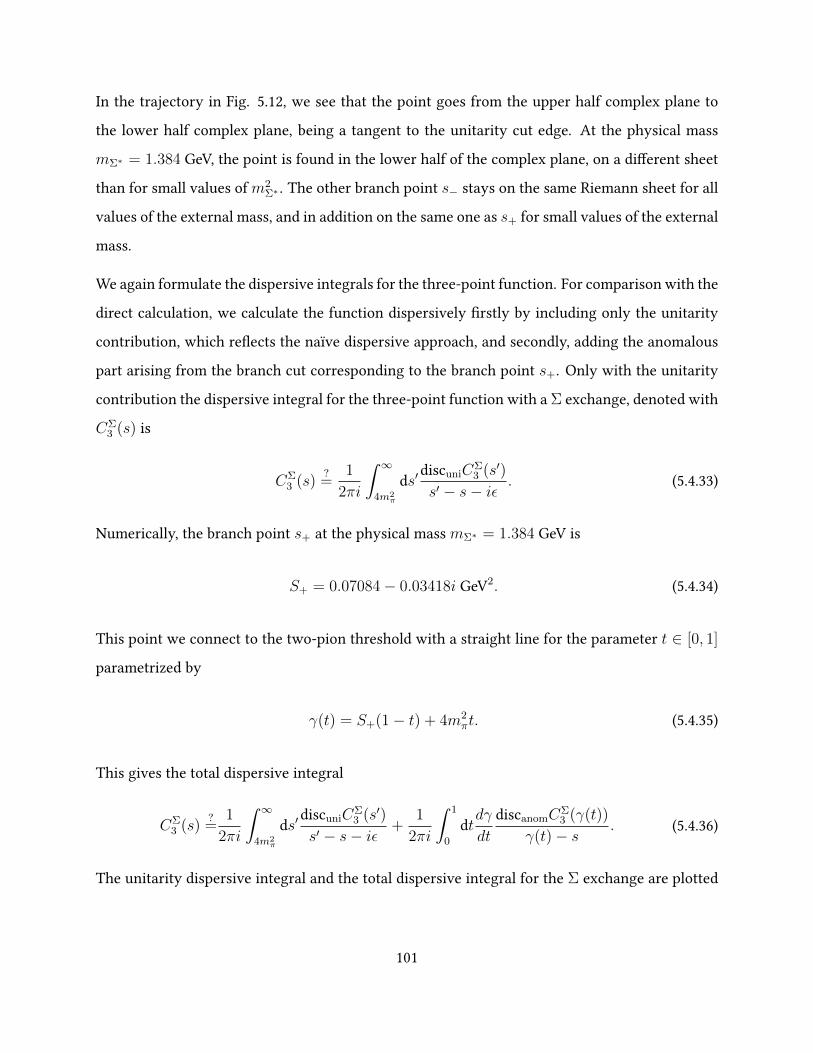
In the trajectory in Fig. 5.12, we see that the point goes from the upper half complex plane to
the lower half complex plane, being a tangent to the unitarity cut edge. At the physical mass
mΣ∗ = 1.384 GeV, the point is found in the lower half of the complex plane, on a dierent sheet
than for small values of m2Σ∗ . The other branch point s− stays on the same Riemann sheet for all
values of the external mass, and in addition on the same one as s+ for small values of the external
mass.
We again formulate the dispersive integrals for the three-point function. For comparison with the
direct calculation, we calculate the function dispersively rstly by including only the unitarity
contribution, which reects the naïve dispersive approach, and secondly, adding the anomalous
part arising from the branch cut corresponding to the branch point s+. Only with the unitarity
contribution the dispersive integral for the three-point function with a Σ exchange, denoted with
CΣ3 (s) is
CΣ3 (s)
?=
1
2πi
∫ ∞4m2
π
ds′discuniC
Σ3 (s′)
s′ − s− iε . (5.4.33)
Numerically, the branch point s+ at the physical mass mΣ∗ = 1.384 GeV is
S+ = 0.07084− 0.03418i GeV2. (5.4.34)
This point we connect to the two-pion threshold with a straight line for the parameter t ∈ [0, 1]
parametrized by
γ(t) = S+(1− t) + 4m2πt. (5.4.35)
This gives the total dispersive integral
CΣ3 (s)
?=
1
2πi
∫ ∞4m2
π
ds′discuniC
Σ3 (s′)
s′ − s− iε +1
2πi
∫ 1
0
dtdγ
dt
discanomCΣ3 (γ(t))
γ(t)− s . (5.4.36)
The unitarity dispersive integral and the total dispersive integral for the Σ exchange are plotted
101
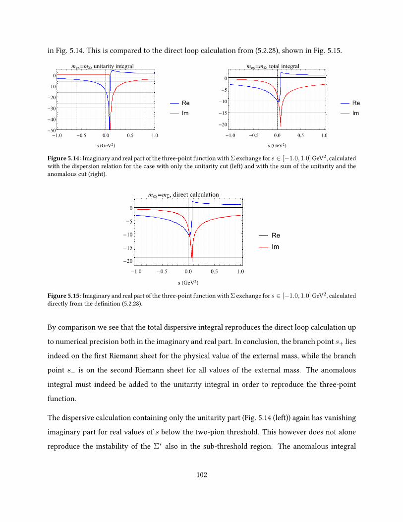
in Fig. 5.14. This is compared to the direct loop calculation from (5.2.28), shown in Fig. 5.15.
-1.0 -0.5 0.0 0.5 1.0-50
-40
-30
-20
-10
0
s (GeV2)
Re
Im
mex=mΣ, unitarity integral
-1.0 -0.5 0.0 0.5 1.0
-20
-15
-10
-5
0
s (GeV2)
Re
Im
mex=mΣ, total integral
Figure 5.14: Imaginary and real part of the three-point function with Σ exchange for s ∈ [−1.0, 1.0] GeV2, calculatedwith the dispersion relation for the case with only the unitarity cut (left) and with the sum of the unitarity and theanomalous cut (right).
-1.0 -0.5 0.0 0.5 1.0
-20
-15
-10
-5
0
s (GeV2)
Re
Im
mex=mΣ, direct calculation
Figure 5.15: Imaginary and real part of the three-point function with Σ exchange for s ∈ [−1.0, 1.0] GeV2, calculateddirectly from the denition (5.2.28).
By comparison we see that the total dispersive integral reproduces the direct loop calculation up
to numerical precision both in the imaginary and real part. In conclusion, the branch point s+ lies
indeed on the rst Riemann sheet for the physical value of the external mass, while the branch
point s− is on the second Riemann sheet for all values of the external mass. The anomalous
integral must indeed be added to the unitarity integral in order to reproduce the three-point
function.
The dispersive calculation containing only the unitarity part (Fig. 5.14 (left)) again has vanishing
imaginary part for real values of s below the two-pion threshold. This however does not alone
reproduce the instability of the Σ∗ also in the sub-threshold region. The anomalous integral
102
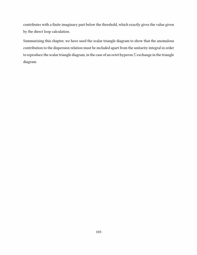
contributes with a nite imaginary part below the threshold, which exactly gives the value given
by the direct loop calculation.
Summarizing this chapter, we have used the scalar triangle diagram to show that the anomalous
contribution to the dispersion relation must be included apart from the unitarity integral in order
to reproduce the scalar triangle diagram, in the case of an octet hyperon Σ exchange in the triangle
diagram.
103
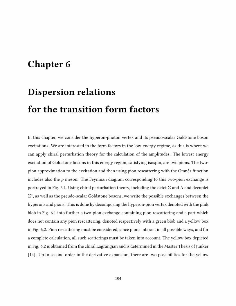
Chapter 6
Dispersion relations
for the transition form factors
In this chapter, we consider the hyperon-photon vertex and its pseudo-scalar Goldstone boson
excitations. We are interested in the form factors in the low-energy regime, as this is where we
can apply chiral perturbation theory for the calculation of the amplitudes. The lowest energy
excitation of Goldstone bosons in this energy region, satisfying isospin, are two pions. The two-
pion approximation to the excitation and then using pion rescattering with the Omnès function
includes also the ρ meson. The Feynman diagram corresponding to this two-pion exchange is
portrayed in Fig. 6.1. Using chiral perturbation theory, including the octet Σ and Λ and decuplet
Σ∗, as well as the pseudo-scalar Goldstone bosons, we write the possible exchanges between the
hyperons and pions. This is done by decomposing the hyperon-pion vertex denoted with the pink
blob in Fig. 6.1 into further a two-pion exchange containing pion rescattering and a part which
does not contain any pion rescattering, denoted respectively with a green blob and a yellow box
in Fig. 6.2. Pion rescattering must be considered, since pions interact in all possible ways, and for
a complete calculation, all such scatterings must be taken into account. The yellow box depicted
in Fig. 6.2 is obtained from the chiral Lagrangian and is determined in the Master Thesis of Junker
[14]. Up to second order in the derivative expansion, there are two possibilities for the yellow
104
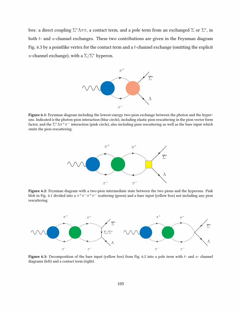
box: a direct coupling Σ∗Λππ, a contact term, and a pole term from an exchanged Σ or Σ∗, in
both t- and u-channel exchanges. These two contributions are given in the Feynman diagram
Fig. 6.3 by a pointlike vertex for the contact term and a t-channel exchange (omitting the explicit
u-channel exchange), with a Σ/Σ∗ hyperon.
π+
π−
Σ∗
Λ
Figure 6.1: Feynman diagram including the lowest-energy two-pion exchange between the photon and the hyper-ons. Indicated is the photon-pion interaction (blue circle), including elastic pion rescattering in the pion vector formfactor, and the Σ∗Λπ+π− interaction (pink circle), also including pion rescattering as well as the bare input whichomits the pion rescattering.
π+
π−
π+
π−
Σ∗
Λ
Figure 6.2: Feynman diagram with a two-pion intermediate state between the two pions and the hyperons. Pinkblob in Fig. 6.1 divided into a π+π−π+π− scattering (green) and a bare input (yellow box) not including any pionrescattering.
π+
π−
π+
π−
Σ∗
Λ
Σ/Σ∗
π+
π−
π+
π−
Σ∗
Λ
Figure 6.3: Decomposition of the bare input (yellow box) from Fig. 6.2 into a pole term with t- and u- channeldiagrams (left) and a contact term (right).
105
Feynman diagrams and therefore also form factors satisfy dispersion relations, as they are analytic
functions of the invariant mass. In the present chapter we present the preliminary results of the
bigger project for which this thesis constitutes a central part: to perform the analytic continuation
of the form factors to the spacelike region via the dispersion relations by using the two-pion
saturation of the hyperon vertex. We present the amplitude for the hyperon-pion vertex using a
once-subtracted dispersion relation and including pion rescattering, using one set of parameters
in the chiral Lagrangian. An unsubtracted dispersion relation calculation for the form factors
Gm(s) is presented, however the tting to the real photon decay width and a calculation for the
parameters yielding a realistic prediction is left as future work and is planned to be presented in
[3].
We consider the unsubtracted dispersion relations for the constrained form factors Gm(s). We
introduce notations for the amplitudes. We denote the ππΣ∗Λ vertex including also the rescat-
tering, denoted with a pink blob in Fig. 6.1 by Tm(s), one for each spin polarization m = 0,±1.
The discontinuity of the form factors is obtained with the optical theorem [5], using only the
two-pion intermediate state. As we are using the p-wave projection, the partial wave decompo-
sition of the amplitude yields an extra factor of pcm (the pion CM momentum) for both the pion
vector form factor and the amplitude Tm, following that of [37, 38]. The discontinuity along the
unitarity cut is
discuniGm(s) = iTm(s)p3
cm(s)F Vπ (s)∗
6π√s
. (6.0.1)
The unsubtracted dispersion relation for the three form factors, m = 0,±1, then reads
Gm(s) =1
12π2
∫ ∞4m2
π
Tm(s′)p3cm(s′)F V
π (s′)∗
s′1/2(s′ − s− iε) +Ganomm (s). (6.0.2)
We express pcm(s) in terms of the Källén function (4.1.22),
pcm(s) =1
2√s
√λ(s,m2
π,m2π) =
1
2
√s− 4m2
π =
√s
2σ(s), (6.0.3)
106
with the denition of σ(s) given in (5.3.19). The piece Ganomm (s) is the dispersive integral along
the anomalous cut in the complex s-plane connecting the branch point S+ and the two-pion
threshold, given explicitly in (5.4.35).
The pion vector form factorF Vπ (s), denoted with a blue blob in Fig. (6.3), includes the information
about the interaction of the pions with the photon. The pion vector form factor is reproduced
to good approximation phenomenologically with the Omnès function Ω(s) (see Section 6.1) by
F Vπ (s) ≈ Ω(s). An even better t used in [38, 39] is when the polynomial in the Omnès problem
(see Section 6.1) is a rst order polynomial,
F Vπ (s) = (1 + αV s)Ω(s), (6.0.4)
with the value αV = 0.12 GeV −2, which reproduces the pion vector form factor to a higher
accuracy.
6.1 Omnès function and pion phase shift
Functions with a discontinuity and a given phase shift over the discontinuity are subject to the
Muskhelishvili-Omnès (M-O) equations [40]. The Omnès problem is treated in detail in various
works [42, 43]. The homogeneous M-O equation for a function F (s) is
ImF (s) = F (s)e−iδ(s)sinδ(s), (6.1.1)
where δ(s) is generally some function describing the phase shift of the function (and is the pion
phase shift in our case). The general solution to the equation is
F (s) = H(s)Ω(s), (6.1.2)
where H(s) is some function and the Omnès function Ω(s) solves (6.1.1) with the boundary
condition Ω(0) = 1. The usage of the Omnès function introduces the pion rescattering [41]
107
in terms of the pion phase shift. The pion phase shift is an observable that is accessible from
experimental data, incorporating the rescattering of the pions.
The exact form of the Omnès function is
Ω(s) = exp(s
π
∫ ∞s0
δ(s′)
s′(s′ − s− iε)ds′)
, s ∈ R. (6.1.3)
We will later need the Omnès function evaluated in the complex s-plane, where we omit the−iεprescription,
Ω(s) = exp(s
π
∫ ∞s0
δ(s′)
s′(s′ − s)ds′)
, s ∈ C. (6.1.4)
The main steps of the derivation of this function are given in Appendix C.
For our case, we are concerned with the l = 1 projection (p-wave) of the amplitude for the pions,
yielding the pion p-wave phase shift. In the article by Garcia-Martin et al. [44], the pion-pion
scattering amplitude is examined, and the phase shifts for dierent waves are presented for dier-
ent energy intervals. For energy regions above 1.42 GeV, Hanhart [45] presents a parametrization
of the pion phase shift so that it reaches π as s → ∞. For the regime above √sedge = 1.4 GeV,
we conduct to the parametrization found in Hanhart’s work [45]. Thus we receive for the p-
wave pion phase shift the following parametrized function, patched together smoothly for three
dierent intervals,
δ1(s) =
cot−1
( √s
2|pcm|3(m2
ρ − s)(
2m3π
m2ρ
√s
+ b0 + b1w(s)
)),√s ≤ 2mK ,
δ1(2mK) + λ1
( √s
2mK
− 1
)+ λ2
( √s
2mK
− 1
)2
, 2mK <√s ≤ √sedge,
π + (δ1(sedge)− π)
(Λ2 + sedge
Λ2 + s
),√sedge <
√s,
(6.1.5)
with
w(s) :=
√s−√s0 − s√s+√s0 − s
for√s0 = 1.5 GeV (6.1.6)
108
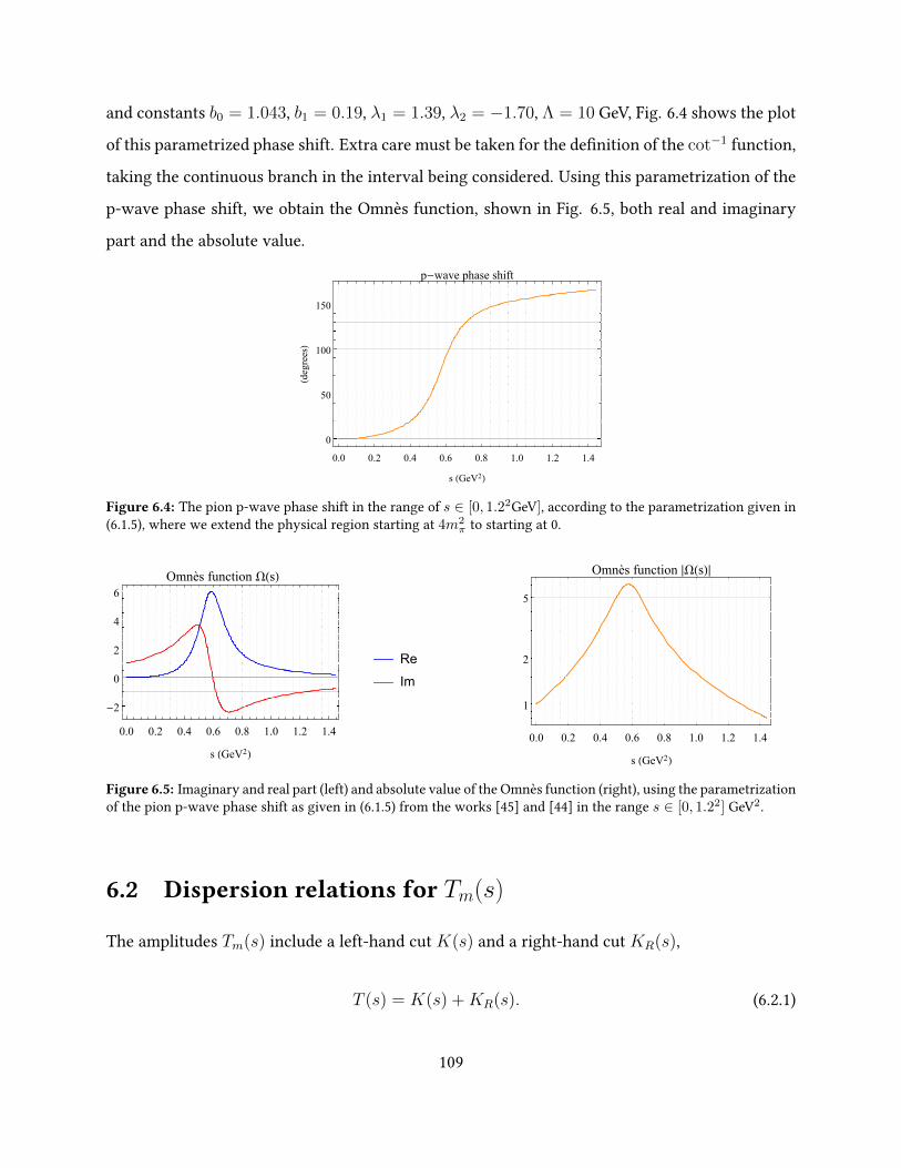
and constants b0 = 1.043, b1 = 0.19, λ1 = 1.39, λ2 = −1.70, Λ = 10 GeV, Fig. 6.4 shows the plot
of this parametrized phase shift. Extra care must be taken for the denition of the cot−1 function,
taking the continuous branch in the interval being considered. Using this parametrization of the
p-wave phase shift, we obtain the Omnès function, shown in Fig. 6.5, both real and imaginary
part and the absolute value.
0.0 0.2 0.4 0.6 0.8 1.0 1.2 1.4
0
50
100
150
s (GeV2)
(degrees)
p-wave phase shift
Figure 6.4: The pion p-wave phase shift in the range of s ∈ [0, 1.22GeV], according to the parametrization given in(6.1.5), where we extend the physical region starting at 4m2
π to starting at 0.
0.0 0.2 0.4 0.6 0.8 1.0 1.2 1.4
-2
0
2
4
6
s (GeV2)
Re
Im
Omnès function Ω(s)
0.0 0.2 0.4 0.6 0.8 1.0 1.2 1.4
1
2
5
s (GeV2)
Omnès function |Ω(s)|
Figure 6.5: Imaginary and real part (left) and absolute value of the Omnès function (right), using the parametrizationof the pion p-wave phase shift as given in (6.1.5) from the works [45] and [44] in the range s ∈ [0, 1.22] GeV2.
6.2 Dispersion relations for Tm(s)
The amplitudes Tm(s) include a left-hand cut K(s) and a right-hand cut KR(s),
T (s) = K(s) +KR(s). (6.2.1)
109
The left-hand cut K(s) is represented by the yellow box in Fig. 6.2 which includes only the
hyperon exchanges. This allows us to see a direct connection between the scalar triangle diagram
and the hyperon exchange diagram, the amplitude K(s). We will make the connection more
explicit later in this section. The right-hand cut has a discontinuity along the unitarity cut, for
which we wish to write the discontinuity along the unitarity cut only, following [38],
Im(T (s)−K(s)) = T (s)e−iδ(s) sin δ(s), (6.2.2)
which is an inhomogeneous M-O equation. For this equation we make the same ansatz as for the
homogeneous case,
T (s)−K(s) = H(s)Ω(s), (6.2.3)
for some function H(s). Substituting in the ansatz (6.2.3) in the inhomogeneous equation (6.2.2)
we get,
Im (Ω(s)H(s)) = (K(s) + Ω(s)H(s))e−iδ(s)sinδ(s). (6.2.4)
Rewriting the left-hand side as the imaginary part of a product,
Re Ω(s)Im H(s) + Im Ω(s)Re H(s) = K(s)e−iδ(s) sin δ(s) +H(s) Ω(s)e−iδ(s)sinδ(s)︸ ︷︷ ︸=Im Ω(s)
,
Re Ω(s)Im H(s) + Im Ω(s) (Re H(s)−H(s))︸ ︷︷ ︸=−i Im H(s)
= K(s)e−iδ(s) sin δ(s),
Im H(s) (Re Ω(s)− i Im Ω(s))︸ ︷︷ ︸|Ω(s)|e−iδ(s)
= K(s)e−iδ(s) sin δ(s),
Im H(s) =K(s) sin δ(s)
|Ω(s)| ,
(6.2.5)
where we have used that Ω(s) satises (6.1.1) and thus also satises Ω(s) = |Ω(s)|eiδ(s).
Having the discontinuity of H(s) (using disc H(s) = 2i Im H(s)), we nally have an n-times
110
subtracted dispersion integral,
H(s) = Pn−1(s) +sn
π
∫ ∞4m2
π
ds′K(s′) sin δ(s′)
|Ω(s′)|s′n(s′ − s− iε) , (6.2.6)
where Pn−1(s) is a polynomial of order n− 1.
Substituting this solution for H(s) in our original ansatz (6.2.3) to the inhomogeneous equation
for T (s), gives the dispersion relation for the amplitude T (s),
T (s) = K(s) + Ω(s)Pn−1(s) + Ω(s)sn
π
∫ ∞4m2
π
ds′K(s′) sin δ(s′)
|Ω(s′)|s′n(s′ − s− iε) , (6.2.7)
which is the dispersion relation for the amplitudes including only the unitarity cut integral. For
the three polarizations m = 0,±1, the three amplitudes Tm are expressed in the same way. The
amplitude Tm(s) are used further in the dispersive integral for the form factorsGm(s). We require
the integrand in the dispersion relation (6.0.2) to vanish for s → ∞, as our formalism works
for low-energy regimes only, and having a contributing part for high energies would invalidate
the method. The Omnès function behaves as ∝ 1s
for large s (see [2]) and so we cannot have a
polynomial Pn−1(s) of higher order than a constant, as this would make the second term in (6.2.7)
divergent for large s.
Finally, based on the analysis of the scalar triangle diagram, we know that an additional anoma-
lous cut is present in the case where we also consider the octet exchange Σ. Thus, we add an
anomalous piece to the integral, T anomm (s), which is expressed as an integral. This gives us nally
with the once-subtracted dispersion relations for the amplitudes Tm(s),
Tm(s) = Km(s)︸ ︷︷ ︸reduced amplitude
+Ω(s)
Pm︸︷︷︸polynomial constant
+s
π
∫ ∞4m2
π
ds′Km(s′) sin δ(s′)
|Ω(s′)|s′(s′ − s− iε)︸ ︷︷ ︸unitarity part
+ T anomm (s)︸ ︷︷ ︸
anomalous part
.
(6.2.8)
The anomalous part is obtained from considering the discontinuity equation, and is described in
111
more detail in [3]. The nal result is
T anomm (s) = s
∫ 1
0
dtdγdt
2fm(γ(t))tIAM(γ(t))
(−λ(γ(t),mΣ∗ ,mΛ)1/2b2(γ(t))Ω(γ(t))(γ(t)− s)γ(t), (6.2.9)
where the path γ(t) is the same parametrization of the anomalous branch cut and the same de-
nition of the branch cut and branch point as used for the scalar triangle case (5.4.35). We use the
pion scattering amplitude in the complex plane tIAM obtained by the inverse amplitude method
by analytic continuation in the complex plane given by Dax et al. [46],
tIAM(s) =t2(s)2
t2(s)− t4(s), (6.2.10)
with the p-wave amplitudes from chiral perturbation theory
t2(s) :=sσ(s)2
96πF 2,
t4(s) := iσ(s)t2(s)2 +t2(s)
48π2F 2
(s
(l +
1
3
)− 15
2m2π−
− 1
2sm4π(41− 2Ls(s)(73− 24σ(s)2) + 3Ls(s)
2(5− 32σ(s)2 + 3σ(s)4))
),
Ls(s) :=1
σ(s)2
(1
2σ(s)log
1 + σ(s)
1− σ(s)− 1
),
(6.2.11)
with the pion decay constant F=0.0868 GeV.
Using chiral perturbation theory, the amplitudes Km(s) can be calculated (see [14]) in terms of
the parameters of the chiral Lagrangian. All constant terms in the amplitudesKm(s) are included
in the subtraction term Pm and so we present the amplitudes with all constant terms subtracted,
K+1 = Coct
(C+1(s) +D+1(s)Roct
s (s))
+ Cdec
(E+1(s) + F+1(s)Rdec
s (s)),
K0 = Coct
(C0(s) +D0(s)Roct
d (s))
+ Cdec
(E0(s) + F0(s)Rdec
d (s)),
K−1 = Coct
(C−1(s) +D−1(s)Roct
s (s))
+ Cdec
(E−1(s) + F−1(s)Rdec
s (s)),
(6.2.12)
where the introduced functions are listed in Appendix D, and the constant parameters Coct and
112
Cdec are dened as
Coct :=DhA
6√
2F 2π
,
Cdec :=HAhA
6√
2F 2π
,
(6.2.13)
where the parameters hA, HA, D are parameters in the chiral Lagrangian [3, 14] and numerical
values are assigned in (6.2.17).
All of the amplitudes Km(s) given in (6.2.12) can be written in the compact form
Km(s) = gm(s) +fm(s)
b(s)b(s)2log
a(s) + b(s)
a(s)− b(s) , (6.2.14)
for some functions fm(s) and gm(s) which do not have any cut intersecting the unitarity cut,
and the functions a(s) and b(s) are as dened earlier for the scalar triangle case (5.3.10) and
we dene b(s) := |b(s)|. This way of rewriting gives the direct analogy to the scalar triangle
case. Comparing (6.2.14) to the unitarity discontinuity of the scalar three-point function (5.3.13),
we see the only dierence being the higher power of b(s) in the denominator of the logarithm
coecient.
From the explicit form (6.2.12) and the functions dened in Appendix D, we may read o the
functions fm(s),
f+1(s) = −CoctD+1(s)(b2(s)− a2(s)),
f0(s) = −CoctD0(s)a(s),
f−1(s) = −CoctD−1(s)(b2(s)− a2(s)),
(6.2.15)
in terms of the parameters of the chiral Lagrangian, given in (6.2.13).
In the expression (6.2.8), we may exert all the constant terms from the amplitudesKm and include
them in the polynomial piece Pm. In addition, the amplitude arising from the contact term de-
picted in Fig. 6.3 (right) will also contribute to a constant term, coming from the next-to-leading
113
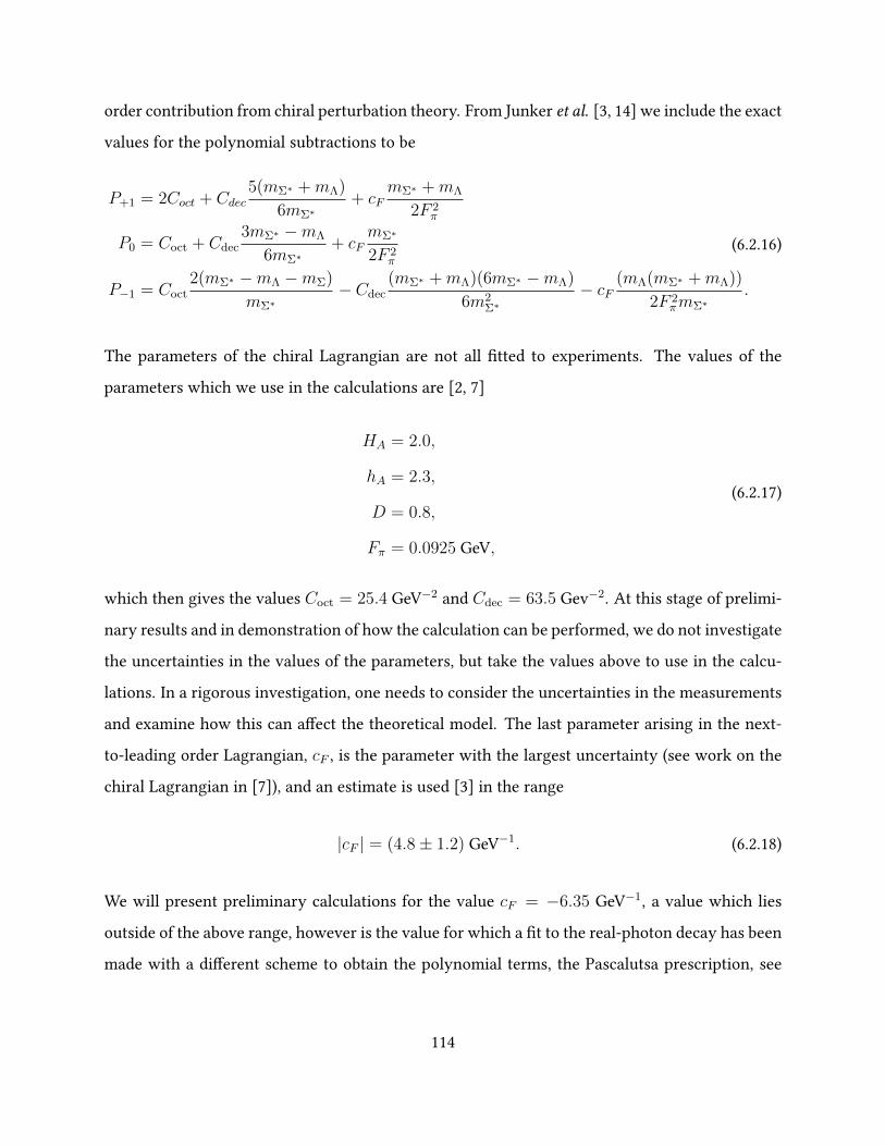
order contribution from chiral perturbation theory. From Junker et al. [3, 14] we include the exact
values for the polynomial subtractions to be
P+1 = 2Coct + Cdec5(mΣ∗ +mΛ)
6mΣ∗+ cF
mΣ∗ +mΛ
2F 2π
P0 = Coct + Cdec3mΣ∗ −mΛ
6mΣ∗+ cF
mΣ∗
2F 2π
P−1 = Coct2(mΣ∗ −mΛ −mΣ)
mΣ∗− Cdec
(mΣ∗ +mΛ)(6mΣ∗ −mΛ)
6m2Σ∗
− cF(mΛ(mΣ∗ +mΛ))
2F 2πmΣ∗
.
(6.2.16)
The parameters of the chiral Lagrangian are not all tted to experiments. The values of the
parameters which we use in the calculations are [2, 7]
HA = 2.0,
hA = 2.3,
D = 0.8,
Fπ = 0.0925 GeV,
(6.2.17)
which then gives the values Coct = 25.4 GeV−2 and Cdec = 63.5 Gev−2. At this stage of prelimi-
nary results and in demonstration of how the calculation can be performed, we do not investigate
the uncertainties in the values of the parameters, but take the values above to use in the calcu-
lations. In a rigorous investigation, one needs to consider the uncertainties in the measurements
and examine how this can aect the theoretical model. The last parameter arising in the next-
to-leading order Lagrangian, cF , is the parameter with the largest uncertainty (see work on the
chiral Lagrangian in [7]), and an estimate is used [3] in the range
|cF | = (4.8± 1.2) GeV−1. (6.2.18)
We will present preliminary calculations for the value cF = −6.35 GeV−1, a value which lies
outside of the above range, however is the value for which a t to the real-photon decay has been
made with a dierent scheme to obtain the polynomial terms, the Pascalutsa prescription, see
114
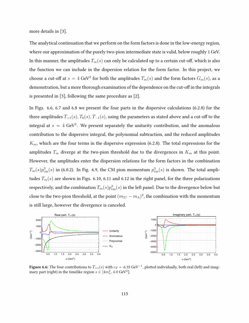
more details in [3].
The analytical continuation that we perform on the form factors is done in the low-energy region,
where our approximation of the purely two-pion intermediate state is valid, below roughly 1 GeV.
In this manner, the amplitudes Tm(s) can only be calculated up to a certain cut-o, which is also
the function we can include in the dispersion relation for the form factor. In this project, we
choose a cut-o at s = 4 GeV2 for both the amplitudes Tm(s) and the form factors Gm(s), as a
demonstration, but a more thorough examination of the dependence on the cut-o in the integrals
is presented in [3], following the same procedure as [2].
In Figs. 6.6, 6.7 and 6.8 we present the four parts in the dispersive calculations (6.2.8) for the
three amplitudes T+1(s), T0(s), T−1(s), using the parameters as stated above and a cut-o to the
integral at s = 4 GeV2. We present separately the unitarity contribution, and the anomalous
contribution to the dispersive integral, the polynomial subtraction, and the reduced amplitudes
Km, which are the four terms in the dispersive expression (6.2.8). The total expressions for the
amplitudes Tm diverge at the two-pion threshold due to the divergences in Km at this point.
However, the amplitudes enter the dispersion relations for the form factors in the combination
Tm(s)p3cm(s) in (6.0.2). In Fig. 6.9, the CM pion momentum p3
cm(s) is shown. The total ampli-
tudes Tm(s) are shown in Figs. 6.10, 6.11 and 6.12 in the right panel, for the three polarizations
respectively, and the combination Tm(s)p3cm(s) in the left panel. Due to the divergence below but
close to the two-pion threshold, at the point (mΣ∗ −mΛ)2, the combination with the momentum
is still large, however the divergence is canceled.
0.5 1.0 1.5 2.0 2.5 3.0 3.5 4.0
-3000
-2000
-1000
0
1000
2000
s (GeV2)
(GeV-2) Unitarity
Anomalous
Polynomial
Km
Real part, T+1(s)
0.5 1.0 1.5 2.0 2.5 3.0 3.5 4.0-5000
-4000
-3000
-2000
-1000
0
1000
s (GeV2)
(GeV-2)
Imaginary part, T+1(s)
Figure 6.6: The four contributions to T+1(s) with cF = -6.35 GeV−1, plotted individually, both real (left) and imag-inary part (right) in the timelike region s ∈ [4m2
π, 4.0 GeV2].
115
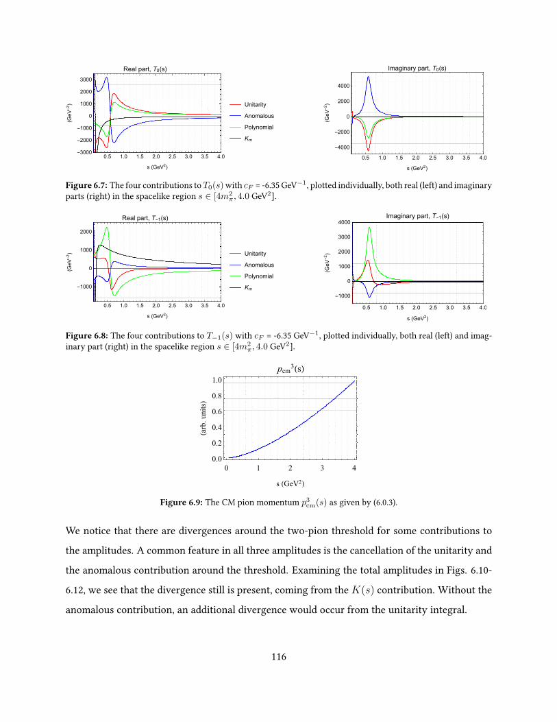
0.5 1.0 1.5 2.0 2.5 3.0 3.5 4.0-3000
-2000
-1000
0
1000
2000
3000
s (GeV2)
(GeV-2) Unitarity
Anomalous
Polynomial
Km
Real part, T0(s)
0.5 1.0 1.5 2.0 2.5 3.0 3.5 4.0
-4000
-2000
0
2000
4000
s (GeV2)
(GeV-2)
Imaginary part, T0(s)
Figure 6.7: The four contributions toT0(s) with cF = -6.35 GeV−1, plotted individually, both real (left) and imaginaryparts (right) in the spacelike region s ∈ [4m2
π, 4.0 GeV2].
0.5 1.0 1.5 2.0 2.5 3.0 3.5 4.0
-1000
0
1000
2000
s (GeV2)
(GeV-2) Unitarity
Anomalous
Polynomial
Km
Real part, T-1(s)
0.5 1.0 1.5 2.0 2.5 3.0 3.5 4.0
-1000
0
1000
2000
3000
4000
s (GeV2)
(GeV-2)
Imaginary part, T-1(s)
Figure 6.8: The four contributions to T−1(s) with cF = -6.35 GeV−1, plotted individually, both real (left) and imag-inary part (right) in the spacelike region s ∈ [4m2
π, 4.0 GeV2].
0 1 2 3 4
0.0
0.2
0.4
0.6
0.8
1.0
s (GeV2)
(arb.units)
pcm3(s)
Figure 6.9: The CM pion momentum p3cm(s) as given by (6.0.3).
We notice that there are divergences around the two-pion threshold for some contributions to
the amplitudes. A common feature in all three amplitudes is the cancellation of the unitarity and
the anomalous contribution around the threshold. Examining the total amplitudes in Figs. 6.10-
6.12, we see that the divergence still is present, coming from the K(s) contribution. Without the
anomalous contribution, an additional divergence would occur from the unitarity integral.
116
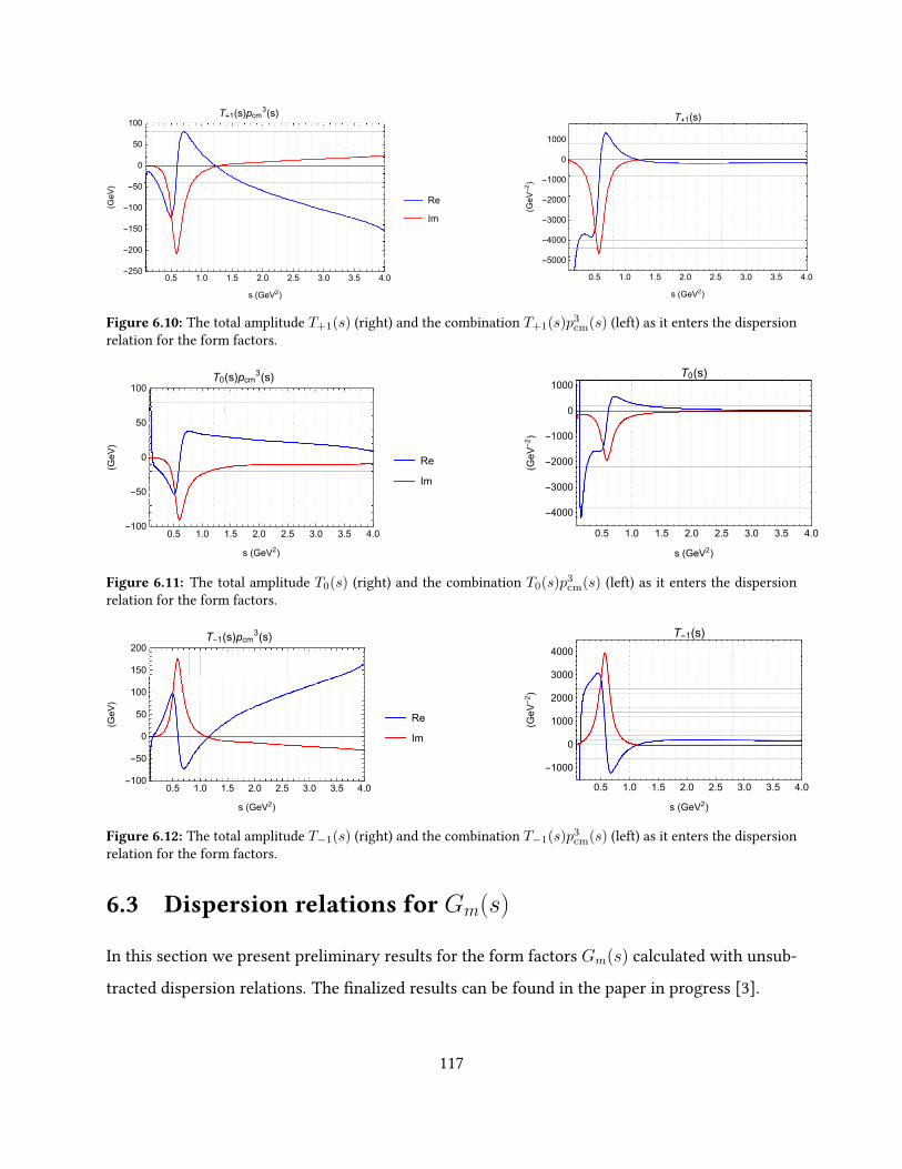
0.5 1.0 1.5 2.0 2.5 3.0 3.5 4.0-250
-200
-150
-100
-50
0
50
100
s (GeV2)
(GeV)
Re
Im
T+1(s)pcm3(s)
0.5 1.0 1.5 2.0 2.5 3.0 3.5 4.0
-5000
-4000
-3000
-2000
-1000
0
1000
s (GeV2)
(GeV-2)
T+1(s)
Figure 6.10: The total amplitude T+1(s) (right) and the combination T+1(s)p3cm(s) (left) as it enters the dispersion
relation for the form factors.
0.5 1.0 1.5 2.0 2.5 3.0 3.5 4.0-100
-50
0
50
100
s (GeV2)
(GeV)
Re
Im
T0(s)pcm3(s)
0.5 1.0 1.5 2.0 2.5 3.0 3.5 4.0
-4000
-3000
-2000
-1000
0
1000
s (GeV2)
(GeV-2)
T0(s)
Figure 6.11: The total amplitude T0(s) (right) and the combination T0(s)p3cm(s) (left) as it enters the dispersion
relation for the form factors.
0.5 1.0 1.5 2.0 2.5 3.0 3.5 4.0-100
-50
0
50
100
150
200
s (GeV2)
(GeV)
Re
Im
T-1(s)pcm3(s)
0.5 1.0 1.5 2.0 2.5 3.0 3.5 4.0
-1000
0
1000
2000
3000
4000
s (GeV2)
(GeV-2)
T-1(s)
Figure 6.12: The total amplitude T−1(s) (right) and the combination T−1(s)p3cm(s) (left) as it enters the dispersion
relation for the form factors.
6.3 Dispersion relations for Gm(s)
In this section we present preliminary results for the form factors Gm(s) calculated with unsub-
tracted dispersion relations. The nalized results can be found in the paper in progress [3].
117
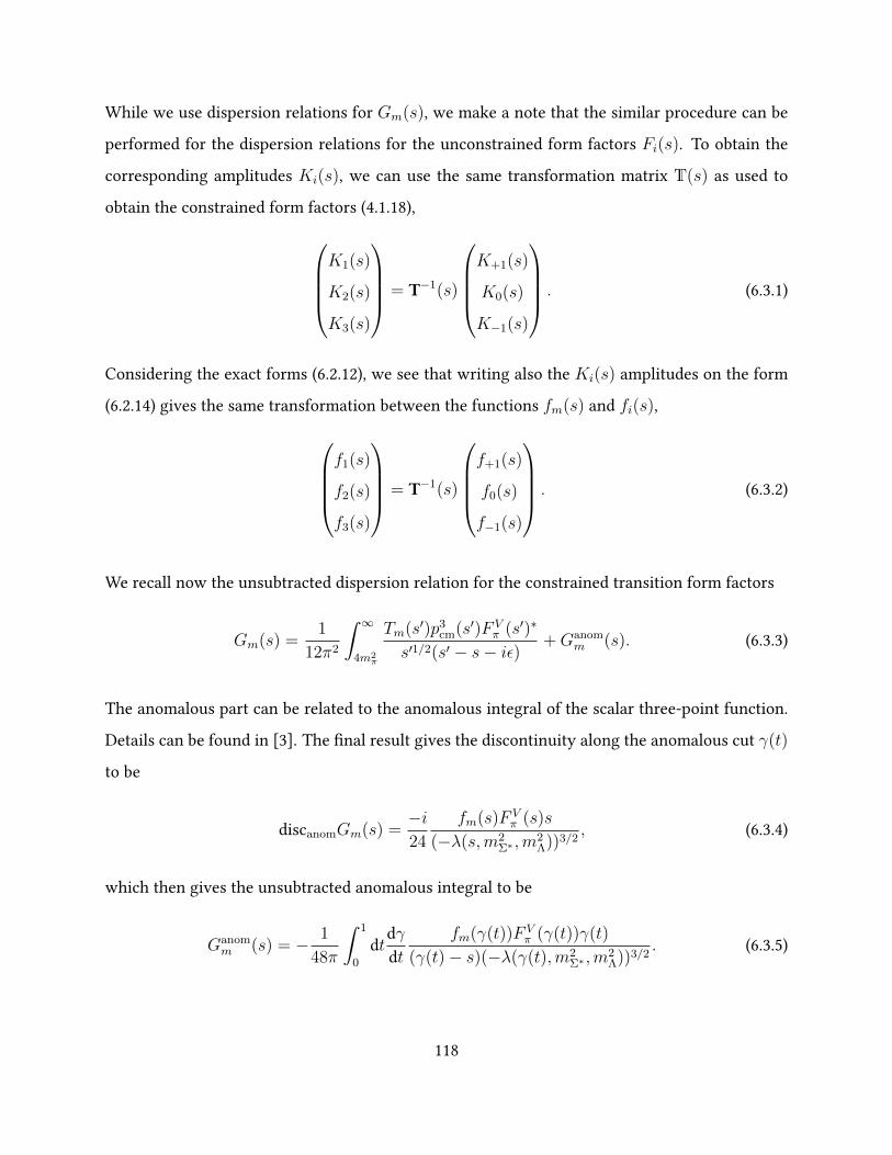
While we use dispersion relations for Gm(s), we make a note that the similar procedure can be
performed for the dispersion relations for the unconstrained form factors Fi(s). To obtain the
corresponding amplitudes Ki(s), we can use the same transformation matrix T(s) as used to
obtain the constrained form factors (4.1.18),K1(s)
K2(s)
K3(s)
= T−1(s)
K+1(s)
K0(s)
K−1(s)
. (6.3.1)
Considering the exact forms (6.2.12), we see that writing also the Ki(s) amplitudes on the form
(6.2.14) gives the same transformation between the functions fm(s) and fi(s),
f1(s)
f2(s)
f3(s)
= T−1(s)
f+1(s)
f0(s)
f−1(s)
. (6.3.2)
We recall now the unsubtracted dispersion relation for the constrained transition form factors
Gm(s) =1
12π2
∫ ∞4m2
π
Tm(s′)p3cm(s′)F V
π (s′)∗
s′1/2(s′ − s− iε) +Ganomm (s). (6.3.3)
The anomalous part can be related to the anomalous integral of the scalar three-point function.
Details can be found in [3]. The nal result gives the discontinuity along the anomalous cut γ(t)
to be
discanomGm(s) =−i24
fm(s)F Vπ (s)s
(−λ(s,m2Σ∗ ,m
2Λ))3/2
, (6.3.4)
which then gives the unsubtracted anomalous integral to be
Ganomm (s) = − 1
48π
∫ 1
0
dtdγdt
fm(γ(t))F Vπ (γ(t))γ(t)
(γ(t)− s)(−λ(γ(t),m2Σ∗ ,m
2Λ))3/2
. (6.3.5)
118
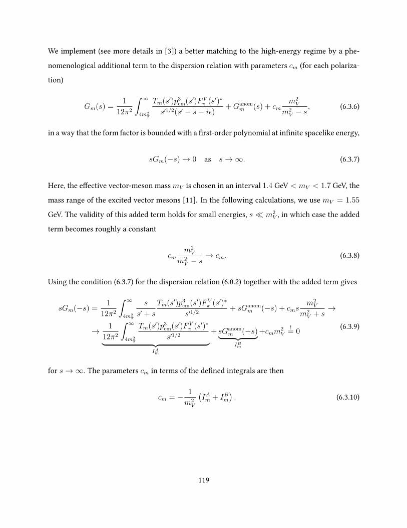
We implement (see more details in [3]) a better matching to the high-energy regime by a phe-
nomenological additional term to the dispersion relation with parameters cm (for each polariza-
tion)
Gm(s) =1
12π2
∫ ∞4m2
π
Tm(s′)p3cm(s′)F V
π (s′)∗
s′1/2(s′ − s− iε) +Ganomm (s) + cm
m2V
m2V − s
, (6.3.6)
in a way that the form factor is bounded with a rst-order polynomial at innite spacelike energy,
sGm(−s)→ 0 as s→∞. (6.3.7)
Here, the eective vector-meson mass mV is chosen in an interval 1.4 GeV < mV < 1.7 GeV, the
mass range of the excited vector mesons [11]. In the following calculations, we use mV = 1.55
GeV. The validity of this added term holds for small energies, s m2V , in which case the added
term becomes roughly a constant
cmm2V
m2V − s
→ cm. (6.3.8)
Using the condition (6.3.7) for the dispersion relation (6.0.2) together with the added term gives
sGm(−s) =1
12π2
∫ ∞4m2
π
s
s′ + s
Tm(s′)p3cm(s′)F V
π (s′)∗
s′1/2+ sGanom
m (−s) + cmsm2V
m2V + s
→
→ 1
12π2
∫ ∞4m2
π
Tm(s′)p3cm(s′)F V
π (s′)∗
s′1/2︸ ︷︷ ︸IAm
+ sGanomm (−s)︸ ︷︷ ︸IBm
+cmm2V
!= 0
(6.3.9)
for s→∞. The parameters cm in terms of the dened integrals are then
cm = − 1
m2V
(IAm + IBm
). (6.3.10)
119
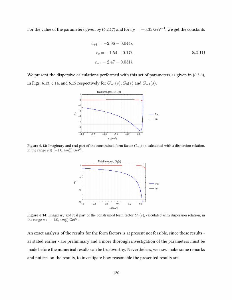
For the value of the parameters given by (6.2.17) and for cF = −6.35 GeV−1, we get the constants
c+1 = −2.96− 0.044i,
c0 = −1.54− 0.17i,
c−1 = 2.47− 0.031i.
(6.3.11)
We present the dispersive calculations performed with this set of parameters as given in (6.3.6),
in Figs. 6.13, 6.14, and 6.15 respectively for G+1(s), G0(s) and G−1(s).
-1.0 -0.8 -0.6 -0.4 -0.2 0.0-6
-5
-4
-3
-2
-1
0
1
s (GeV2)
G+1
Re
Im
Total integral, G+1(s)
Figure 6.13: Imaginary and real part of the constrained form factor G+1(s), calculated with a dispersion relation,in the range s ∈ [−1.0, 4m2
π) GeV2.
-1.0 -0.8 -0.6 -0.4 -0.2 0.0-15
-10
-5
0
s (GeV2)
G0
Re
Im
Total integral, G0(s)
Figure 6.14: Imaginary and real part of the constrained form factor G0(s), calculated with dispersion relation, inthe range s ∈ [−1.0, 4m2
π) GeV2.
An exact analysis of the results for the form factors is at present not feasible, since these results -
as stated earlier - are preliminary and a more thorough investigation of the parameters must be
made before the numerical results can be trustworthy. Nevertheless, we now make some remarks
and notices on the results, to investigate how reasonable the presented results are.
120
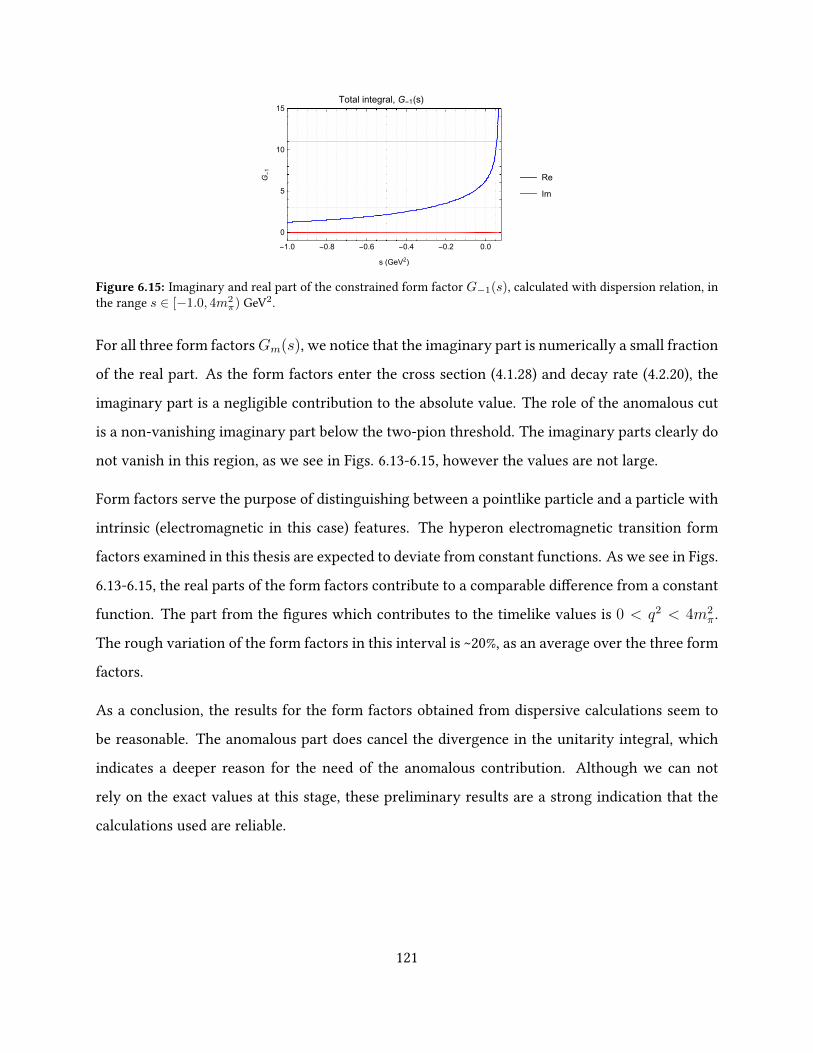
-1.0 -0.8 -0.6 -0.4 -0.2 0.0
0
5
10
15
s (GeV2)G
-1
Re
Im
Total integral, G-1(s)
Figure 6.15: Imaginary and real part of the constrained form factor G−1(s), calculated with dispersion relation, inthe range s ∈ [−1.0, 4m2
π) GeV2.
For all three form factorsGm(s), we notice that the imaginary part is numerically a small fraction
of the real part. As the form factors enter the cross section (4.1.28) and decay rate (4.2.20), the
imaginary part is a negligible contribution to the absolute value. The role of the anomalous cut
is a non-vanishing imaginary part below the two-pion threshold. The imaginary parts clearly do
not vanish in this region, as we see in Figs. 6.13-6.15, however the values are not large.
Form factors serve the purpose of distinguishing between a pointlike particle and a particle with
intrinsic (electromagnetic in this case) features. The hyperon electromagnetic transition form
factors examined in this thesis are expected to deviate from constant functions. As we see in Figs.
6.13-6.15, the real parts of the form factors contribute to a comparable dierence from a constant
function. The part from the gures which contributes to the timelike values is 0 < q2 < 4m2π.
The rough variation of the form factors in this interval is ~20%, as an average over the three form
factors.
As a conclusion, the results for the form factors obtained from dispersive calculations seem to
be reasonable. The anomalous part does cancel the divergence in the unitarity integral, which
indicates a deeper reason for the need of the anomalous contribution. Although we can not
rely on the exact values at this stage, these preliminary results are a strong indication that the
calculations used are reliable.
121
Chapter 7
Conclusions and outlook
Summarizing the thesis, rstly, the interaction Lagrangian for the electromagnetic interaction
with the two hyperons Σ∗ and Λ was constructed, based on the internal symmetries of the theory.
In addition, the vertex function was constructed, in terms of the three electromagnetic transition
form factors. In terms of these, the dierential cross section of the e+e− → Σ∗Λ reaction was
calculated, as well as the dierential decay rate of Σ∗ → Λe+e−, and the total decay rate for
the real-photon decay Σ∗ → Λγ. These predictions are expressions which may in the future be
compared to experimental data from for example HADES and PANDA at FAIR. The decay rate
for the real-photon decay may be used to pin down the parameters of the theory, and hence make
the theory one which can predict future reactions.
We approximated the hyperon-photon vertex with a two-pion intermediate state, leading to a
diagram with the pion vector form factor, a ππ → ππ scattering, and a part including only the
exchange of a hyperon and a direct hyperon-pion contact term. This approximation led to a
triangle diagram with two pions and an exchanged hyperon as a propagator. The anomalous cut
arises when the mass of the exchanged particle is light enough compared to the external masses,
which is the case for the Σ exchange.
The scalar triangle diagram was used as a simple model for the examination of the analytic struc-
ture of the form factors. We found the unitarity discontinuity to dene two Riemann sheets. For
122
physical values of the external and internal masses, the branch points of the logarithm in the
discontinuity were found to be located on two dierent Riemann sheets in the case of the Σ ex-
change. By evaluating the dispersive integral for the cases including and excluding the anomalous
cut, we found that the anomalous piece is indeed needed to reconstruct the exact loop diagram
for the Σ exchange. This calculation then utilized the usage of the anomalous contribution in the
dispersion relations for the form factors Gm(s).
This work constitutes a central part of a paper which is in progress [3]. The outlook for this
paper and this topic, is the tting of the form factors to the experimental values planned to be
measured by HADES and PANDA at FAIR. This way, the parameters used in the chiral Lagrangian
can be tted to match experiment, which can give an accurate prediction of the form factors in
the spacelike region. Presently, a good access to the spacelike region of the form factors is via
dispersion relations, for unstable particles such as the Σ∗. Timelike region measurements are
planned to be performed, and these can in the future be tted to the predictions of the decay rate
and cross section in terms of the transition form factors.
The method of using dispersion relations for calculation of form factors is based on the assump-
tion of the analyticity of the form factors and amplitudes. While this assumption can be made,
the framework can be applied on any form factors. Each special case in addition brings in unique
features arising from the physics behind the particles and reactions. In the prevailing case, the
special feature which needs extra examination is the anomalous cut. Anomalous cuts are present
also in other decays and the present work can be used as an initial step towards it. Other decays
may reveal further interesting mathematical and physical insights into the behavior of Nature.
123

Appendices
124
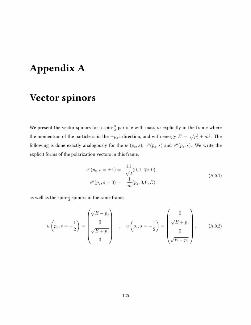
Appendix A
Vector spinors
We present the vector spinors for a spin-32
particle with mass m explicitly in the frame where
the momentum of the particle is in the +pz z direction, and with energy E =√p2z +m2. The
following is done exactly analogously for the uµ(pz, s), vµ(pz, s) and vµ(pz, s). We write the
explicit forms of the polarization vectors in this frame,
εµ(pz, s = ±1) =±1√
2(0, 1,∓i, 0),
εµ(pz, s = 0) =1
m(pz, 0, 0, E),
(A.0.1)
as well as the spin-12
spinors in the same frame,
u
(pz, s = +
1
2
)=
√E − pz
0√E + pz
0
, u
(pz, s = −1
2
)=
0
√E + pz
0√E − pz.
. (A.0.2)
125
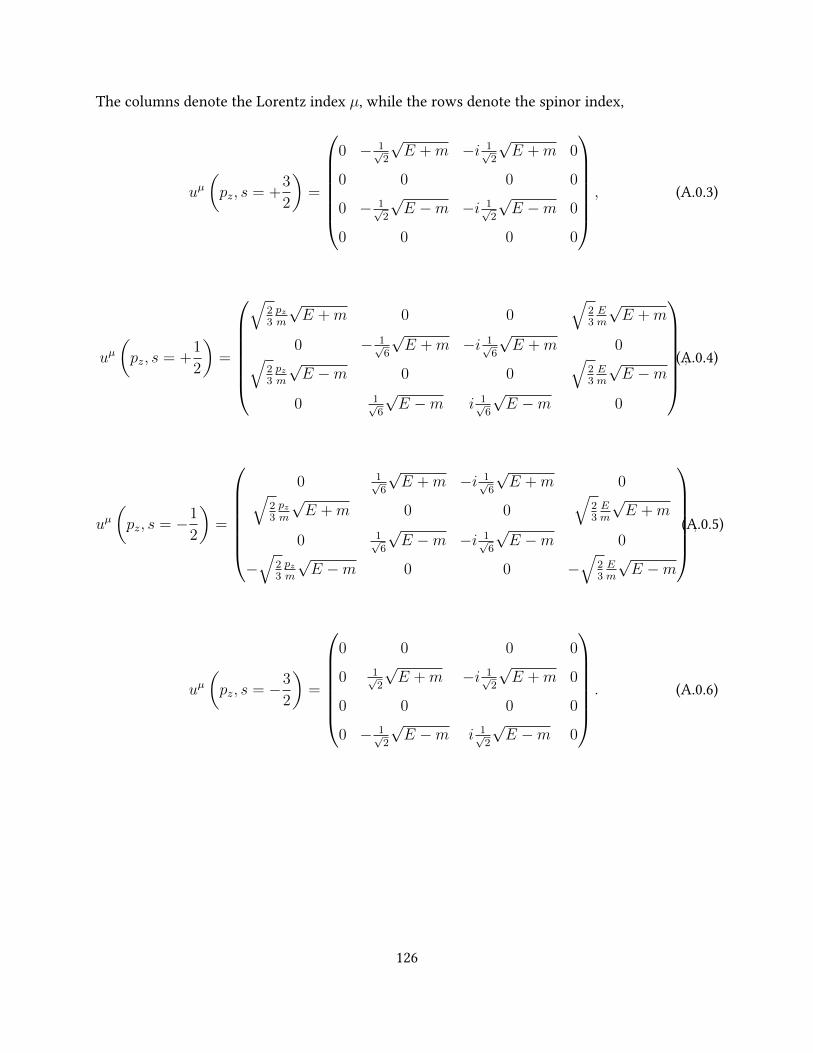
The columns denote the Lorentz index µ, while the rows denote the spinor index,
uµ(pz, s = +
3
2
)=
0 − 1√
2
√E +m −i 1√
2
√E +m 0
0 0 0 0
0 − 1√2
√E −m −i 1√
2
√E −m 0
0 0 0 0
, (A.0.3)
uµ(pz, s = +
1
2
)=
√23pzm
√E +m 0 0
√23Em
√E +m
0 − 1√6
√E +m −i 1√
6
√E +m 0√
23pzm
√E −m 0 0
√23Em
√E −m
0 1√6
√E −m i 1√
6
√E −m 0
,(A.0.4)
uµ(pz, s = −1
2
)=
0 1√
6
√E +m −i 1√
6
√E +m 0√
23pzm
√E +m 0 0
√23Em
√E +m
0 1√6
√E −m −i 1√
6
√E −m 0
−√
23pzm
√E −m 0 0 −
√23Em
√E −m
,(A.0.5)
uµ(pz, s = −3
2
)=
0 0 0 0
0 1√2
√E +m −i 1√
2
√E +m 0
0 0 0 0
0 − 1√2
√E −m i 1√
2
√E −m 0
. (A.0.6)
126
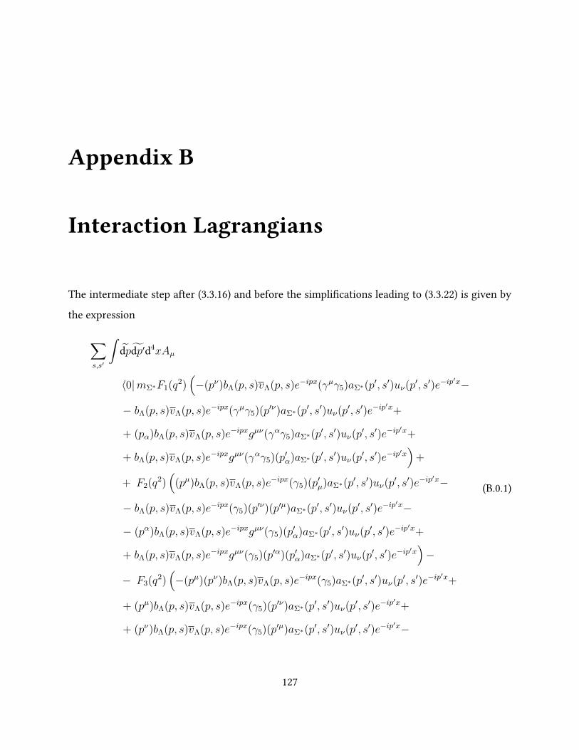
Appendix B
Interaction Lagrangians
The intermediate step after (3.3.16) and before the simplications leading to (3.3.22) is given by
the expression
∑s,s′
∫dpdp′d4xAµ
〈0|mΣ∗F1(q2)(−(pν)bΛ(p, s)vΛ(p, s)e−ipx(γµγ5)aΣ∗(p
′, s′)uν(p′, s′)e−ip
′x−
− bΛ(p, s)vΛ(p, s)e−ipx(γµγ5)(p′ν)aΣ∗(p′, s′)uν(p
′, s′)e−ip′x+
+ (pα)bΛ(p, s)vΛ(p, s)e−ipxgµν(γαγ5)aΣ∗(p′, s′)uν(p
′, s′)e−ip′x+
+ bΛ(p, s)vΛ(p, s)e−ipxgµν(γαγ5)(p′α)aΣ∗(p′, s′)uν(p
′, s′)e−ip′x)
+
+ F2(q2)(
(pµ)bΛ(p, s)vΛ(p, s)e−ipx(γ5)(p′µ)aΣ∗(p′, s′)uν(p
′, s′)e−ip′x−
− bΛ(p, s)vΛ(p, s)e−ipx(γ5)(p′ν)(p′µ)aΣ∗(p′, s′)uν(p
′, s′)e−ip′x−
− (pα)bΛ(p, s)vΛ(p, s)e−ipxgµν(γ5)(p′α)aΣ∗(p′, s′)uν(p
′, s′)e−ip′x+
+ bΛ(p, s)vΛ(p, s)e−ipxgµν(γ5)(p′α)(p′α)aΣ∗(p′, s′)uν(p
′, s′)e−ip′x)−
− F3(q2)(−(pµ)(pν)bΛ(p, s)vΛ(p, s)e−ipx(γ5)aΣ∗(p
′, s′)uν(p′, s′)e−ip
′x+
+ (pµ)bΛ(p, s)vΛ(p, s)e−ipx(γ5)(p′ν)aΣ∗(p′, s′)uν(p
′, s′)e−ip′x+
+ (pν)bΛ(p, s)vΛ(p, s)e−ipx(γ5)(p′µ)aΣ∗(p′, s′)uν(p
′, s′)e−ip′x−
(B.0.1)
127
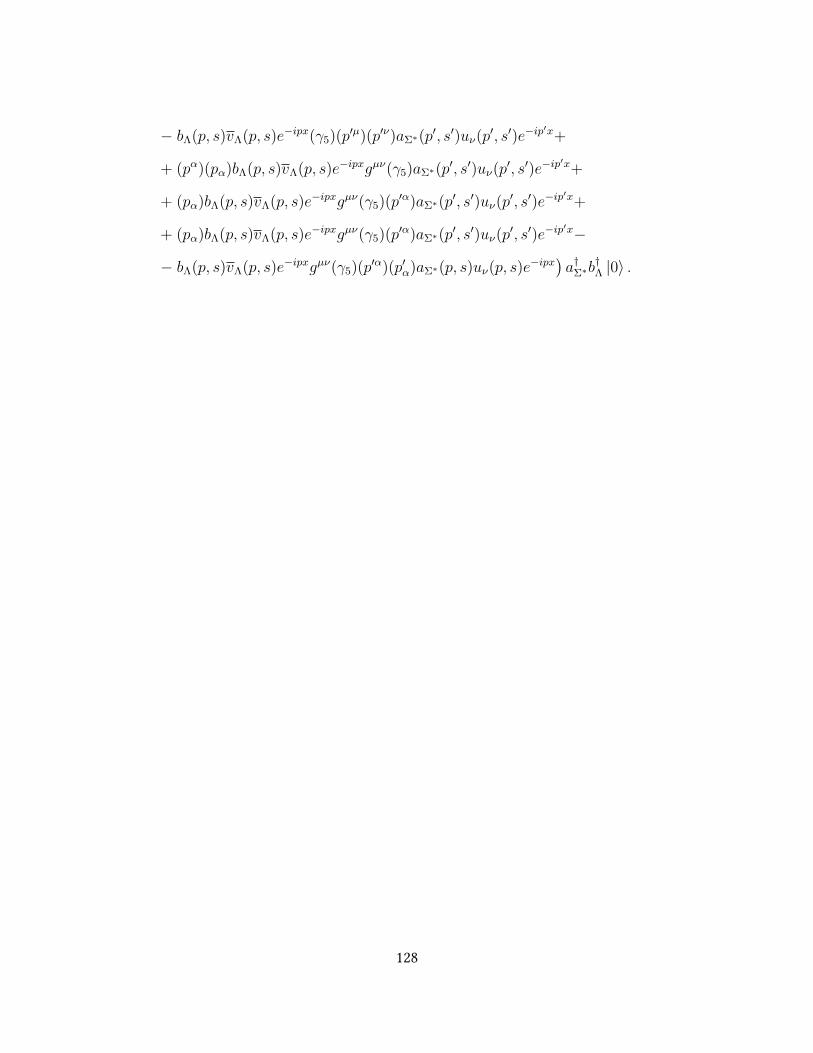
− bΛ(p, s)vΛ(p, s)e−ipx(γ5)(p′µ)(p′ν)aΣ∗(p′, s′)uν(p
′, s′)e−ip′x+
+ (pα)(pα)bΛ(p, s)vΛ(p, s)e−ipxgµν(γ5)aΣ∗(p′, s′)uν(p
′, s′)e−ip′x+
+ (pα)bΛ(p, s)vΛ(p, s)e−ipxgµν(γ5)(p′α)aΣ∗(p′, s′)uν(p
′, s′)e−ip′x+
+ (pα)bΛ(p, s)vΛ(p, s)e−ipxgµν(γ5)(p′α)aΣ∗(p′, s′)uν(p
′, s′)e−ip′x−
− bΛ(p, s)vΛ(p, s)e−ipxgµν(γ5)(p′α)(p′α)aΣ∗(p, s)uν(p, s)e−ipx) a†Σ∗b†Λ |0〉 .
128
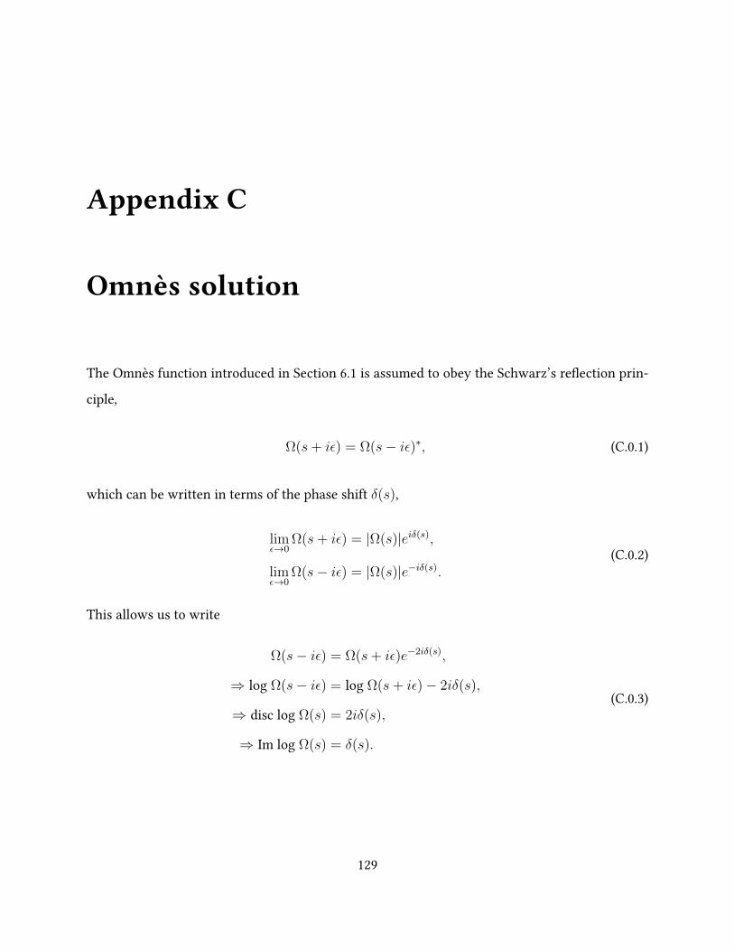
Appendix C
Omnès solution
The Omnès function introduced in Section 6.1 is assumed to obey the Schwarz’s reection prin-
ciple,
Ω(s+ iε) = Ω(s− iε)∗, (C.0.1)
which can be written in terms of the phase shift δ(s),
limε→0
Ω(s+ iε) = |Ω(s)|eiδ(s),
limε→0
Ω(s− iε) = |Ω(s)|e−iδ(s).(C.0.2)
This allows us to write
Ω(s− iε) = Ω(s+ iε)e−2iδ(s),
⇒ log Ω(s− iε) = log Ω(s+ iε)− 2iδ(s),
⇒ disc log Ω(s) = 2iδ(s),
⇒ Im log Ω(s) = δ(s).
(C.0.3)
129
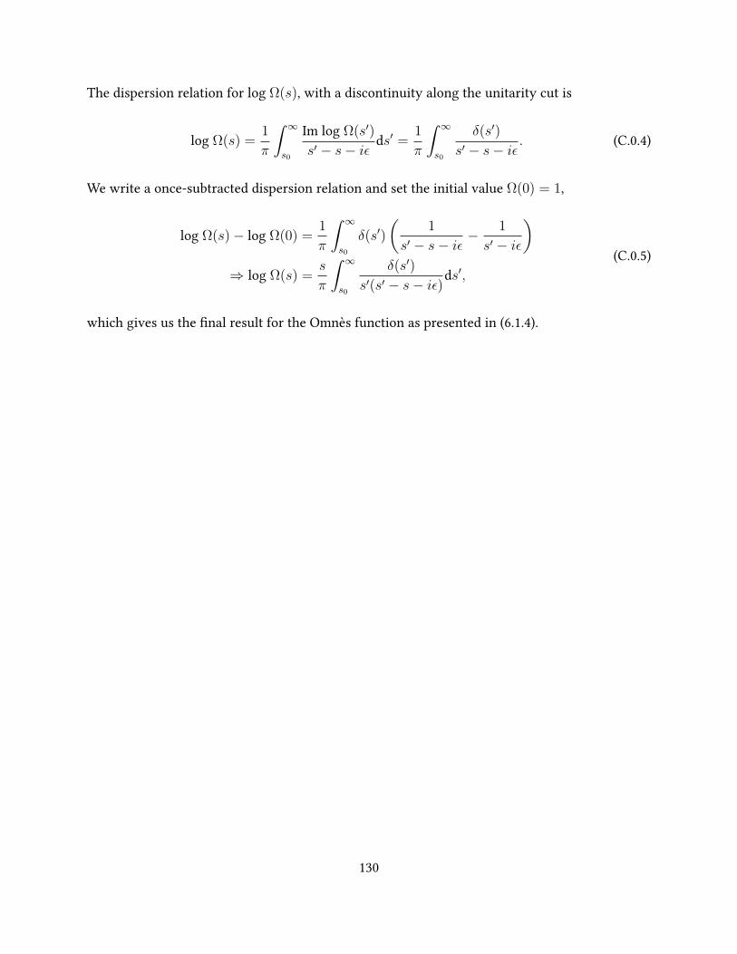
The dispersion relation for log Ω(s), with a discontinuity along the unitarity cut is
log Ω(s) =1
π
∫ ∞s0
Im log Ω(s′)
s′ − s− iε ds′ =1
π
∫ ∞s0
δ(s′)
s′ − s− iε . (C.0.4)
We write a once-subtracted dispersion relation and set the initial value Ω(0) = 1,
log Ω(s)− log Ω(0) =1
π
∫ ∞s0
δ(s′)
(1
s′ − s− iε −1
s′ − iε
)⇒ log Ω(s) =
s
π
∫ ∞s0
δ(s′)
s′(s′ − s− iε)ds′,(C.0.5)
which gives us the nal result for the Omnès function as presented in (6.1.4).
130
Appendix D
Amplitude functions
The functions introduced in (6.2.12) are given by
Rocts (s) =
4
b2(s)− 4
aΣ(s)
b2(s)|b(s)|
(tan−1 |b(s)|
aΣ(s)+ πΘ(scr − s)
),
Roctd (s) = −2
aΣ(s)
b2(s)− 2
b2(s)− a2Σ(s)
b2(s)|b(s)|
(tan−1 |b(s)|
aΣ(s)+ πΘ(scr − s)
),
Rdecs (s) = −2
aΣ∗(s)
b2(s)− 2
b2(s)− a2Σ∗(s)
b2(s)|b(s)|
(tan−1 |b(s)|
aΣ∗(s)
),
Rdecd (s) = 4
1
b2(s)− 4
aΣ∗(s)
b2(s)|b(s)| tan−1 |b(s)|aΣ∗(s)
,
(D.0.1)
with a(s) being the function dened in (5.3.13) with the subscript denoting which exchanged
particle it considers (mex = mΣ or mex = mΣ∗). The function b(s) is as dened in (5.3.13).
The rest of the functions are
C+1(s) = −2(mΣ∗ −mΛ)(mΛ +mΣ)
s− (mΣ∗ −mΛ)2,
C0(s) =(mΣ∗ +mΛ)(mΣ∗ +mΣ)
s− 3mΣ∗(mΛ +mΣ)
s− (mΣ∗ −mΛ)2,
C−1(s) = −6(mΣ∗ −mΛ)(mΛ +mΣ)
s− (mΣ∗ −mΛ)2,
(D.0.2)
131
D+1(s) = 3mΣ(mΣ +mΛ) +(3(mΣ∗ −mΛ)(mΛ +mΣ)(m2
π +mΣ∗mΛ −m2Σ))
s− (mΣ∗ −mΛ)2,
D0(s) = 3mΣ(mΛ +mΣ)(m2Σ∗ −mΣ∗mΣ −m2
π +m2Σ)− 9mΣ∗(mΛ +mΣ)(mΣ∗mΛ +m2
π −m2Σ)
s− (mΣ∗ −mΛ)2+
+3(mΣ∗ +mΛ)(mΣ +mΛ)
s
(m3
Σ∗mΛ −mΣ(mΣ∗ −mΛ)(m2Σ∗ +m2
π) + 2m2Σ∗m
2π−
−m2Σ(mΣ∗(mΣ∗ +mΛ) + 2m2
π) + 2mΣ∗mΛm2π −m3
Σ(mΛ −mΣ∗) +m4π +m4
Σ
),
D−1(s) =3
mΣ∗(mΛ +mΣ)(m2
π −m2Σ∗ +mΣ∗mΣ −m2
Σ)+
+9(mΣ∗ −mΛ)(mΛ +mΣ)(m2
π +mΣ∗mΛ −m2Σ)
s− (mΣ∗ −mΛ)2,
E+1(s) =(mΣ∗ −mΛ)((mΣ∗ +mΛ)2 −m2
π)
3mΣ∗(s− (mΣ∗ −mΛ)2),
E0(s) = −(mΛ +mΣ∗)(2m2Σ∗ + 2mΛmΣ∗ −m2
π)
6mΣ∗s+
(mΛ +mΣ∗)2 −m2
π
2(s− (mΣ∗ +mΛ)2,
E−1(s) =(mΣ∗ −mΛ)((mΣ∗ +mΛ)2 −m2
π)
mΣ∗(s− (mΣ∗ −mΛ)2),
F+1(s) = −3s
2− m2
π(2mΣ∗ + 3mΛ)
2mΣ∗+
5(mΣ∗ +mΛ)2
2+
+(mΣ∗ −mΛ)((mΣ∗ +mΛ)2 −m2
π)(m2Σ∗ −mΣ∗mΛ −m2
π)
2mΣ∗(s− (mΣ∗ +mΛ)2),
F0(s) = m4π +
3m2Σ∗s
2− m2
π(7m2Σ∗ − 2mΣ∗mΛ + 2m2
Λ) +m2Σ∗(mΣ∗ +mΛ)2
2+
+4m2
Σ∗m2π(mΣ∗ − 2mΛ)(mΣ∗ +mΛ)2 −m4
π(2m3Σ∗ +m2
Σ∗mΛ +m3Λ) +m6
π(mΣ∗ +mΛ)
2mΣ∗s+
+3((mΣ∗ +mΛ)2 −m2
π)(mΣ∗(mΛ −mΣ∗) +m2π))2
2(s− (mΣ∗ −m2Λ)
,
F−1(s) =3s
2+m2π(m2
Σ∗ +mΣ∗mΛ −m2Λ) +m4
π
2m2Σ∗
− 5(mΣ∗ +mΛ)2
2+
+3(mΣ∗ −mΛ)((mΣ∗ +mΛ)2 −m2
π)(m2Σ∗ −mΣ∗mΛ −m2
π)
2mΣ∗(s− (mΣ∗ −mΛ)2).
(D.0.3)
132
Bibliography
[1] K. Schönning and C. Li. Future perspectives on baryon form factor measurements with BES
III. EPJ Web of Conferences 137, 12002 (2017).
[2] C. Granados, S. Leupold and E. Perotti. The electromagnetic Sigma-to-Lambda hyperon tran-
sition form factors at low energies. Eur. Phys. J., A 53, 117 (2017).
[3] O. Junker, S. Leupold, E. Perotti and T. Vitos, Uppsala University, in preparation (2019).
[4] M. Srednicki. Quantum Field Theory, Cambridge University Press, 2012.
[5] M. E. Peskin and D. V. Schroeder. Introduction to Quantum Field Theory, Westview Press, 1995.
[6] S. Weinberg. The Quantum Theory of Fields, Cambridge University Press, 1995.
[7] M. Holmberg and S. Leupold. The relativistic chiral Lagrangian for decuplet and octet baryons
at next-to-leading order. Eur. Phys. J., A 54, 103 (2018).
[8] E. Perotti, G. Fäldt, A. Kupsc, S. Leupold and J. J. Song. Polarization observables in e+e−
annihilation to a baryon-antibaryon pair. Phys. Rev., D 99, 056008 (2019).
[9] W. Rarita and J. Schwinger. On a theory of particles with half-integer spin. Phys. Rev. 60, 61
(1941).
[10] U. Mosel. Fields, Symmetries and Quarks, Springer, 2012.
[11] C. Patrignani et al. (Particle Data Group), Chin. Phys., C 40, 100001 (2016) and 2018 update.
[12] S. Scherer and M. R. Schindler. A Primer for Chiral Perturbation Theory, Springer, 2012.
133
[13] J. Gasser and H. Leutwyler. Chiral perturbation theory to one loop. Annals Phys., 158, 142
(1984).
[14] O. Junker. Master Thesis. Uppsala University, in preparation.
[15] J. Feltesse. Introduction to deep inelastic scattering: past and present. XX International work-
shop on deep-inelastic scattering and related subjects, Bonn, Germany, March 2012.
[16] C. E. Carlsson. Electromagnetic N −∆ transition at high Q2. Phys. Rev., D 34, 2704 (1986).
[17] F. E. Close and W. N. Cottingham. The kinematic and symmetry structure of e+e− →hadron
pairs. Nucl. Phys., B 99, 61 (1975).
[18] E. L. Lomon and S. Pacetti. Timelike and spacelike electromagnetic form factors of nucleons,
a unied description. Phys. Rev., D 85, 113004 (2012).
[19] B. Kubis and U.-G. Meissner. Baryon form factors in chiral perturbation theory. Eur. Phys.
J., C 18, 747 (2001).
[20] R. Karplus, C. M. Sommereld and E. H. Wichmann. Spectral representations in perturbation
theory. I. Vertex function. Phys. Rev. 111, 1187 (1958).
[21] K. Schönning. Strong interaction studies with PANDA at FAIR. EPJ Web of Conferences 125,
01006 (2016).
[22] B. Ramstein. Time-like baryon transitions studies with HADES. EPJ Web. Conf., 199, 01008
(2019).
[23] M. Jacob and G. V. Wick. On the general theory of collisions for particles with spin. Annals
Phys., 281, 774 (2000).
[24] J. G. Körner and M. Kuroda. e+e− annihilation into baryon-antibaryon pairs. Phys. Rev. D
16, 2165 (1977).
[25] G. ’t Hooft and M. Veltman. Scalar one-loop integrals. Nucl. Phys. B 153, 365 (1979).
[26] T. W. Gamelin. Complex analysis, Springer, 2001.
134
[27] R. Zwicky. A Brief Introduction to Dispersion relations and analyticity. Strong Fields and
Heavy Quarks, Dubna, Russia, July 2016. arXiv:1610.06090 [hep-ph]
[28] J. F. Donoghue. Dispersion relations and eective eld theory. International School on Eec-
tive Field Theory, Almunecar, Spain, June 1995. arXiv:hep-ph/9607351 [hep-ph]
[29] R. E. Cutkosky. Singularities and Discontinuities of Feynman Amplitudes. J. of Math. Phys.,
1, 429 (1960).
[30] H. Elvang and Y. Husang. Scattering Amplitudes. (2014). arXiv:1308.1697 [hep-th] (2014).
[31] H. J. Lu and C. A. Perez. Massless one-loop scalar three-point integral and associated
Clausen, Glaisher and L-functions. SLAC-PUB, 5809 (1992).
[32] L. G. Cabral-Rosetti and M. A. Sanchis-Lozano. Appell functions and the scalar one-loop
three-point integrals in Feynman diagrams. J. Phys.: Conf. Ser., 37, 82 (2006).
[33] H. Ghaderi. Project Thesis. Uppsala University, (2013).
[34] B. Moussallam. Couplings of light I=0 scalar mesons to simple operators in the complex
plane. Phys. J., C 71, 1814 (2011).
[35] W. Lucha, D. Melikhov and S. Simula. Dispersion representations and anomalous singulari-
ties of the triangle diagram. Phys. Rev., D 75, 016001 (2007).
[36] W. Lucha, D. Melikhov and S. Simula. Erratum: Dispersion representations and anomalous
singularities of the triangle diagram. Phys. Rev., D 92, 019901(E) (2015).
[37] G. Köpp. Dispersion calculation of the transition form factor Fπωγ(t) with cut contributions.
Phys. Rev., D 10, 932 (1974).
[38] S. Leupold. The nucleon as a test case to calculate vector-isovector form factors at low en-
ergies. Eur. Phys. J. A 54, 1 (2018).
135
[39] M. Hoferichter, B. Kubis, J. Ruiz de Elvira, H.-W. Hammer and U.-G. Meissner. On the ππ
continuum in the nucleon form factors and the proton radius puzzle. Eur. Phys. J. A 52, 331
(2016).
[40] Y. Iwamura. A method of solution to Muskhelishvili-Omnès equation in nal-state interac-
tion model. Prog. Theor. Phys., 56, 1812 (1976).
[41] G. Colangelo, J. Gasser and H. Leutwyler. ππ scattering. Nucl. Phys., B 603, 125 (2001).
[42] A. V. Anisovich and H. Leutwyler. Dispersive analysis of the decay η → 3π. Phys. Lett., B
375, 335 (1996).
[43] F. Niecknig, B. Kubis and S. P. Schneider. Dispersive analysis of ω → 3π and φ → 3π. Eur.
Phys. J. C 72, 2014 (2012).
[44] R. Garcia-Martin, R. Kaminski, J. R. Peláez, J. R de Elvira and F. J. Ynduráin. The pion-pion
scattering amplitude IV: Improved Analysis with Once Subtracted Roy-Like Equations up to
1100 MeV. Phys. Rev., D 83, 074004 (2011).
[45] C. Hanhart. A new parametrization for the pion vector form factor. Phys. Lett., B 715, 170
(2012).
[46] M. Dax, T. Isken and B. Kubis. Quark-mass dependence in ω → 3π decays. Eur. Phys. J., C
78, 859 (2018).
136