vv v v v v v v vv vv vv () ( ) - Center for Advanced Studies of...
13
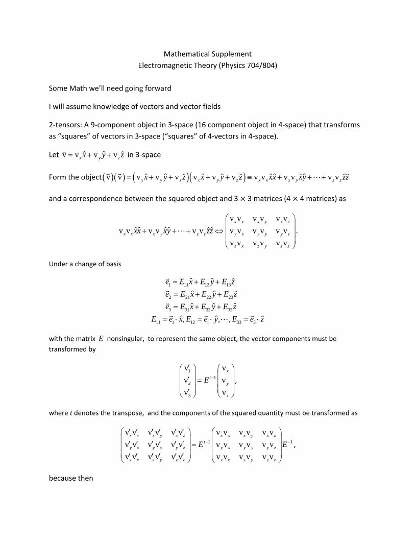
Mathematical Supplement Electromagnetic Theory (Physics 704/804) Some Math we’ll need going forward I will assume knowledge of vectors and vector fields 2‐tensors: A 9‐component object in 3‐space (16 component object in 4‐space) that transforms as “squares” of vectors in 3‐space (“squares” of 4‐vectors in 4‐space). Let ˆ ˆ ˆ v v v v x y z x y z = + + r in 3‐space Form the object ( )( ) ( ) ( ) ˆ ˆ ˆ ˆ ˆˆ ˆˆ ˆ ˆ ˆˆ v v v v v v v v vv vv vv x y z x y z x x x y z z x y z x y z xx xy zz = + + + + ≡ + + + r r L and a correspondence between the squared object and 3 3 matrices (4 4 matrices) as vv vv vv ˆˆ ˆˆ ˆˆ vv vv vv vv vv vv vv vv vv x x x y x z x x x y z z y x y y y z z x z y z z xx xy zz ⎛ ⎞ ⎜ ⎟ + + + ⇔ ⎜ ⎟ ⎜ ⎟ ⎝ ⎠ L . Under a change of basis 1 11 12 13 2 21 22 23 3 31 32 33 11 1 12 1 33 3 ˆ ˆ ˆ ˆ ˆ ˆ ˆ ˆ ˆ ˆ ˆ ˆ , , , e Ex E y Ez e Ex E y Ez e Ex E y Ez E e xE e y E e z = + + = + + = + + = ⋅ = ⋅ = ⋅ r r r r r r L with the matrix E nonsingular, to represent the same object, the vector components must be transformed by 1 1 2 3 v v v v v v x t y z E − ′ ⎛ ⎞ ⎛ ⎞ ⎜ ⎟ ⎜ ⎟ ′ = ⎜ ⎟ ⎜ ⎟ ⎜ ⎟ ⎜ ⎟ ′ ⎝ ⎠ ⎝ ⎠ , where t denotes the transpose, and the components of the squared quantity must be transformed as 1 1 vv vv vv vv vv vv vv vv vv vv vv vv vv vv vv vv vv vv x x x y x z x x x y x z t y x y y y z y x y y y z z x z y z z z x z y z z E E − − ′′ ′ ′ ′′ ⎛ ⎞ ⎛ ⎞ ⎜ ⎟ ⎜ ⎟ ′ ′ ′ ′ ′ ′ = ⎜ ⎟ ⎜ ⎟ ⎜ ⎟ ⎜ ⎟ ′′ ′′ ′′ ⎝ ⎠ ⎝ ⎠ , because then
Transcript of vv v v v v v v vv vv vv () ( ) - Center for Advanced Studies of...
Mathematical Supplement Electromagnetic Theory (Physics 704/804)
Some Math we’ll need going forward
I will assume knowledge of vectors and vector fields
2‐tensors: A 9‐component object in 3‐space (16 component object in 4‐space) that transforms as “squares” of vectors in 3‐space (“squares” of 4‐vectors in 4‐space).
Let ˆ ˆ ˆv v v vx y zx y z= + +r
in 3‐space
Form the object ( )( ) ( )( )ˆ ˆ ˆ ˆ ˆ ˆ ˆˆˆ ˆ ˆˆv v v v v v v v v v v v v vx y z x y z x x x y z zx y z x y z xx xy zz= + + + + ≡ + + +r r
L
and a correspondence between the squared object and 3 3 matrices (4 4 matrices) as
v v v v v vˆˆ ˆˆ ˆˆv v v v v v v v v v v v
v v v v v v
x x x y x z
x x x y z z y x y y y z
z x z y z z
xx xy zz⎛ ⎞⎜ ⎟
+ + + ⇔ ⎜ ⎟⎜ ⎟⎝ ⎠
L .
Under a change of basis
1 11 12 13
2 21 22 23
3 31 32 33
11 1 12 1 33 3
ˆ ˆ ˆ ˆ ˆ ˆ ˆ ˆ ˆ
ˆ ˆ ˆ, , ,
e E x E y E ze E x E y E ze E x E y E z
E e x E e y E e z
= + += + += + +
= ⋅ = ⋅ = ⋅
r
r
r
r r rL
with the matrix E nonsingular, to represent the same object, the vector components must be transformed by
1
12
3
v vv vv v
xt
y
z
E −
′⎛ ⎞ ⎛ ⎞⎜ ⎟ ⎜ ⎟′ =⎜ ⎟ ⎜ ⎟⎜ ⎟ ⎜ ⎟′⎝ ⎠ ⎝ ⎠
,
where t denotes the transpose, and the components of the squared quantity must be transformed as
1 1
v v v v v v v v v v v vv v v v v v v v v v v vv v v v v v v v v v v v
x x x y x z x x x y x zt
y x y y y z y x y y y z
z x z y z z z x z y z z
E E− −
′ ′ ′ ′ ′ ′⎛ ⎞ ⎛ ⎞⎜ ⎟ ⎜ ⎟′ ′ ′ ′ ′ ′ =⎜ ⎟ ⎜ ⎟⎜ ⎟ ⎜ ⎟′ ′ ′ ′ ′ ′⎝ ⎠ ⎝ ⎠
,
because then
1 1 1 1 1 2 1 2 3 3 3 3 ˆ ˆ ˆˆ ˆˆv v v v v v v v v v v vx x x z z ze e e e e e xx xy zz′ ′ ′ ′ ′ ′+ + + = + + +r r r r r r
L L .
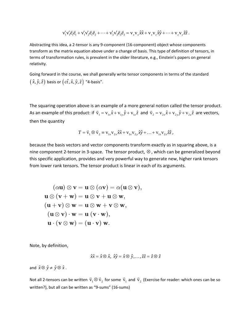
Abstracting this idea, a 2‐tensor is any 9‐component (16‐component) object whose components transform as the matrix equation above under a change of basis. This type of definition of tensors, in terms of transformation rules, is prevalent in the older literature, e.g., Einstein’s papers on general relativity.
Going forward in the course, we shall generally write tensor components in terms of the standard
( )ˆ ˆ ˆ, ,x y z basis or ( )ˆ ˆ ˆ ˆ, , ,ct x y z “4‐basis”.
The squaring operation above is an example of a more general notion called the tensor product.
As an example of this product: if 1 1 1 1ˆ ˆ ˆv v v vx y zx y z= + +r
and 2 2 2 2ˆ ˆ ˆv v v vx y zx y z= + +r
are vectors,
then the quantity
1 2 1 2 1 2 1 2ˆ ˆ ˆˆ ˆˆv v v v v v v vx x x y z zT xx xy zz= ⊗ ≡ + + +r r
K ,
because the basis vectors and vector components transform exactly as in squaring above, is a nine component 2‐tensor in 3‐space. The tensor product, ⊗ , which can be generalized beyond this specific application, provides and very powerful way to generate new, higher rank tensors from lower rank tensors. The tensor product is linear in each of its arguments.
Note, by definition,
ˆ ˆ ˆ ˆ ˆˆ ˆ ˆ ˆˆ ˆ ˆ, , ,xx x x xy x y zz z z= ⊗ = ⊗ = ⊗K
and ˆ ˆ ˆ ˆx y y x⊗ ≠ ⊗ .
Not all 2‐tensors can be written 1 2v v⊗r r
for some 1vr and 2vr (Exercise for reader: which ones can be so
written?), but all can be written as “9‐sums” (16‐sums)
11 12 33ˆ ˆ ˆˆ ˆˆT t xx t xy t zz= + + +L
for some real numbers ijt , called the components of the tensor in the standard basis, where i
and j extend from 1 to 3 (0 to 3). To prove this assertion note that if the 2‐tensor is dotted into
the standard basis vectors
11 12 33ˆ ˆ ˆ ˆ ˆ ˆ, , , t x T x t x T y t z T z= ⋅ ⋅ = ⋅ ⋅ = ⋅ ⋅L , then 11 12 33ˆ ˆ ˆˆ ˆˆT t xx t xy t zz= + + +L .
The components are sometimes written in matrix form
11 12 13
21 22 23
31 32 33
t t tt t tt t t
⎛ ⎞⎜ ⎟⎜ ⎟⎜ ⎟⎝ ⎠
, or for 4‐space
00 01 02 03
10 11 12 13
20 21 22 23
30 31 32 33
t t t tt t t tt t t tt t t t
⎛ ⎞⎜ ⎟⎜ ⎟⎜ ⎟⎜ ⎟⎝ ⎠
,
and manipulated as a single entity.
Relationship between 3 by 3 matrices, 2‐tensors, and bi‐linear maps. Set up a correspondence
( ) ( )( )
( ) ( )( )
( ) ( )
ˆ ˆ 1 2 1 2 1 2
ˆˆ 1 2 1 2 1 2
ˆˆ 1 2 1
1 0 0ˆˆ ˆ ˆ0 0 0 v , v v v v v
0 0 0
0 1 0ˆˆ ˆ ˆ0 0 0 v , v v v v v
0 0 0
0 0 0ˆˆ ˆ ˆ0 0 0 v , v v
0 0 1
xx x x
xy x y
zz
xx T x x
xy T x y
zz T z z
⎛ ⎞⎜ ⎟⇔ ⇔ = ⋅ ⋅ =⎜ ⎟⎜ ⎟⎝ ⎠⎛ ⎞⎜ ⎟⇔ ⇔ = ⋅ ⋅ =⎜ ⎟⎜ ⎟⎝ ⎠
⎛ ⎞⎜ ⎟⇔ ⇔ = ⋅⎜ ⎟⎜ ⎟⎝ ⎠
r r r r
r r r r
M
r r r ( )2 1 2v v vz z⋅ =r
Each of which is obviously bi‐linear. Any bi‐linear map 3 3: R R RL × → , can be represented by a matrix, and hence by a corresponding tensor by expanding analogously to above. Let
( ) ( ) ( )11 12 33ˆ ˆ ˆ ˆ ˆ ˆ, , , , , ,l L x x l L x y l L z z= = =L , then 11 12 33ˆ ˆ ˆˆ ˆˆL l xx l xy l zz= + + +L
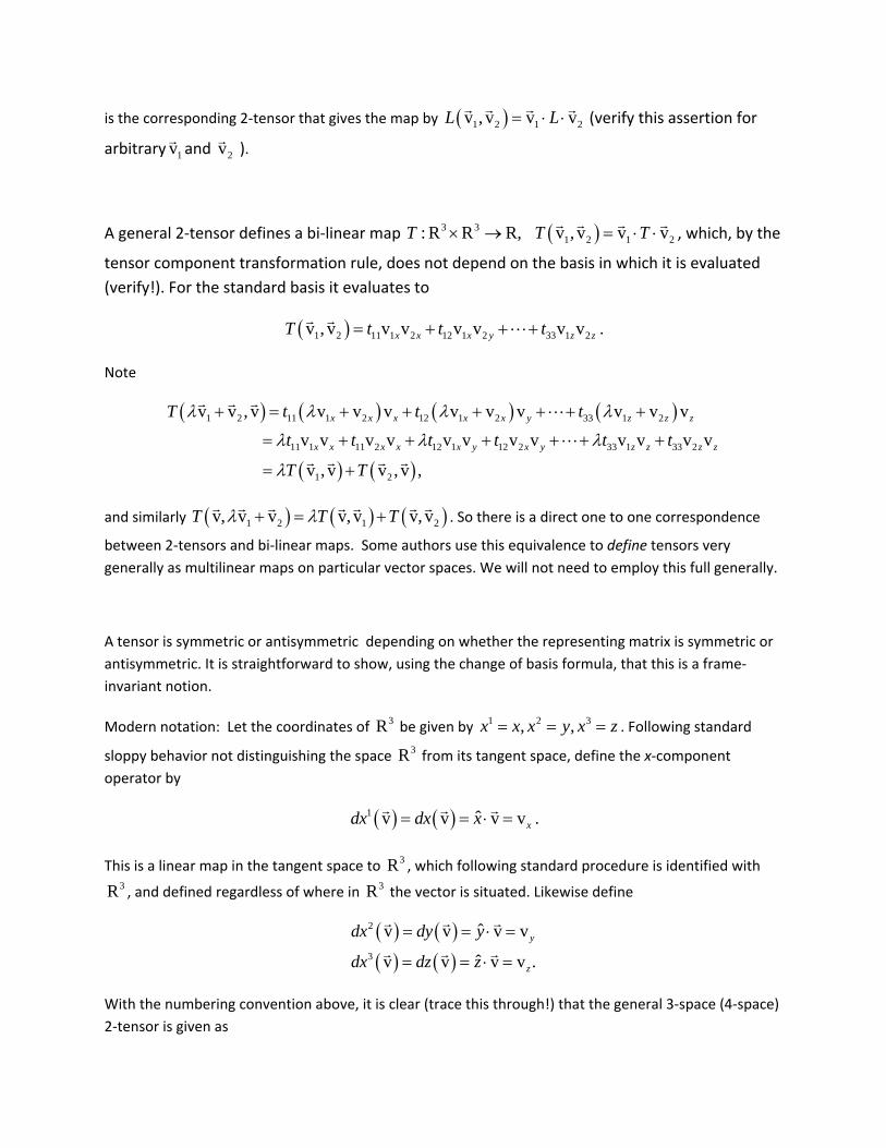
is the corresponding 2‐tensor that gives the map by ( )1 2 1 2v , v v vL L= ⋅ ⋅r r r r
(verify this assertion for
arbitrary 1vr and 2vr ).
A general 2‐tensor defines a bi‐linear map ( )3 31 2 1 2: R R R, v , v v vT T T× → = ⋅ ⋅r r r r
, which, by the
tensor component transformation rule, does not depend on the basis in which it is evaluated (verify!). For the standard basis it evaluates to
( )1 2 11 1 2 12 1 2 33 1 2v , v v v v v v vx x x y z zT t t t= + + +r r
L .
Note
( ) ( ) ( ) ( )
( ) ( )
1 2 11 1 2 12 1 2 33 1 2
11 1 11 2 12 1 12 2 33 1 33 2
1 2
v v , v v v v v v v v v v
v v v v v v v v v v v v
v , v v , v ,
x x x x x y z z z
x x x x x y x y z z z z
T t t t
t t t t t t
T T
λ λ λ λ
λ λ λ
λ
+ = + + + + + +
= + + + + + +
= +
r r rL
Lr r r r
and similarly ( ) ( ) ( )1 2 1 2v, v v v, v v, vT T Tλ λ+ = +r r r r r r r
. So there is a direct one to one correspondence
between 2‐tensors and bi‐linear maps. Some authors use this equivalence to define tensors very generally as multilinear maps on particular vector spaces. We will not need to employ this full generally.
A tensor is symmetric or antisymmetric depending on whether the representing matrix is symmetric or antisymmetric. It is straightforward to show, using the change of basis formula, that this is a frame‐invariant notion.
Modern notation: Let the coordinates of 3R be given by 1 2 3, ,x x x y x z= = = . Following standard
sloppy behavior not distinguishing the space 3R from its tangent space, define the x‐component operator by
( ) ( )1 ˆv v v vxdx dx x= = ⋅ =r r r
.
This is a linear map in the tangent space to 3R , which following standard procedure is identified with 3R , and defined regardless of where in 3R the vector is situated. Likewise define
( ) ( )( ) ( )
2
3
ˆv v v v
ˆv v v v .y
z
dx dy y
dx dz z
= = ⋅ =
= = ⋅ =
r r r
r r r
With the numbering convention above, it is clear (trace this through!) that the general 3‐space (4‐space) 2‐tensor is given as
,i jijT t dx dx= ⊗
where i and j are summed from 1 to 3 (0 to 3). Going forward, the following Einstein summation will
be followed. When an upper and lower latin index is used, the summation index goes from 1 to 3. When an upper and lower greek index is used, the sum proceeds from 0 (representing the time coordinate) to 3.
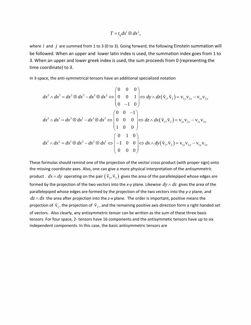
In 3‐space, the anti‐symmetrical tensors have an additional specialized notation
( )
( )
( )
2 3 2 3 3 21 2 1 2 1 2
3 1 3 1 1 31 2 1 2 1 2
1 2 1 2 2 11 2
0 0 00 0 1 v , v v v v v0 1 0
0 0 10 0 0 v , v v v v v1 0 0
0 1 01 0 0 v , v
0 0 0
y z z y
z x x z
dx dx dx dx dx dx dy dz
dx dx dx dx dx dx dz dx
dx dx dx dx dx dx dx dy
⎛ ⎞⎜ ⎟∧ = ⊗ − ⊗ ⇔ ⇔ ∧ = −⎜ ⎟⎜ ⎟−⎝ ⎠
−⎛ ⎞⎜ ⎟∧ = ⊗ − ⊗ ⇔ ⇔ ∧ = −⎜ ⎟⎜ ⎟⎝ ⎠⎛ ⎞⎜ ⎟∧ = ⊗ − ⊗ ⇔ − ⇔ ∧ =⎜ ⎟⎜ ⎟⎝ ⎠
r r
r r
r r1 2 1 2v v v vx y y x−
These formulas should remind one of the projection of the vector cross product (with proper sign) onto the missing coordinate axes. Also, one can give a more physical interpretation of the antisymmetric
product . dx dy∧ operating on the pair ( )1 2v , vr r gives the area of the parallelepiped whose edges are
formed by the projection of the two vectors into the x‐y plane. Likewise dy dz∧ gives the area of the
parallelepiped whose edges are formed by the projection of the two vectors into the y‐z plane, and
dz dx∧ the area after projection into the z‐x plane. The order is important, positive means the
projection of 1vr , the projection of 2vr , and the remaining positive axis direction form a right handed set
of vectors. Also clearly, any antisymmetric tensor can be written as the sum of these three basis tensors. For four space, 2‐ tensors have 16 components and the antisymmetic tensors have up to six independent components. In this case, the basic antisymmetric tensors are
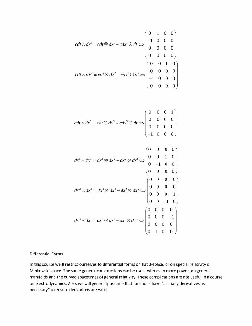
1 1 1
2 2 2
0 1 0 01 0 0 0
0 0 0 00 0 0 0
0 0 1 00 0 0 01 0 0 0
0 0 0 0
cdt dx cdt dx cdx dt
cdt dx cdt dx cdx dt
⎛ ⎞⎜ ⎟−⎜ ⎟∧ = ⊗ − ⊗ ⇔⎜ ⎟⎜ ⎟⎝ ⎠⎛ ⎞⎜ ⎟⎜ ⎟∧ = ⊗ − ⊗ ⇔⎜ ⎟−⎜ ⎟⎝ ⎠
3 3 3
1 2 1 2 2 1
2 3 2 3 3 2
3 1 3 1 1 3
0 0 0 10 0 0 00 0 0 01 0 0 0
0 0 0 00 0 1 00 1 0 00 0 0 0
0 0 0 00 0 0 00 0 0 10 0 1 0
0 0 0 00 0 0 10 0 0 00 1 0 0
cdt dx cdt dx cdx dt
dx dx dx dx dx dx
dx dx dx dx dx dx
dx dx dx dx dx dx
⎛ ⎞⎜ ⎟⎜ ⎟∧ = ⊗ − ⊗ ⇔⎜ ⎟⎜ ⎟−⎝ ⎠
⎛ ⎞⎜ ⎟⎜ ⎟∧ = ⊗ − ⊗ ⇔⎜ ⎟−⎜ ⎟⎝ ⎠⎛ ⎞⎜ ⎟⎜ ⎟∧ = ⊗ − ⊗ ⇔⎜ ⎟⎜ ⎟
−⎝ ⎠
−∧ = ⊗ − ⊗ ⇔
⎛ ⎞⎜ ⎟⎜ ⎟⎜ ⎟⎜ ⎟⎝ ⎠
Differential Forms
In this course we’ll restrict ourselves to differential forms on flat 3‐space, or on special relativity’s Minkowski space. The same general constructions can be used, with even more power, on general manifolds and the curved spacetimes of general relativity. These complications are not useful in a course on electrodynamics. Also, we will generally assume that functions have “as many derivatives as necessary” to ensure derivations are valid.
A differentiable function 3: R Rf → will be called a 0‐form.
A 1‐form is any mapping, linear on vector spaces, of the form
( )( ) ( ) ( )( ) ( ) ( )( )( ) ( )( )
1 1 21 2
33
v , , , , v , , , , v , ,
, , v , , ,
x y z a x y z dx x y z a x y z dx x y z
a x y z dx x y z
ω = +
+
r r r
r ,
where the ia are differentiable functions, and as above, the idx project out specific components of the
vector field at the location in question. 1‐forms operate on vector fields and yield a scalar (i.e., basis independent) 0‐form on evaluation with a specific vector field.
A 2‐form is the analogous construction applied to antisymmetric 2‐tensor fields. It is a bi‐linear anti‐symmetric mapping of the form
( ) ( ) ( )( )
2 2 3 3 11 2 1 1 2 2 1 2
1 23 1 2
v , v v , v v , v
v , v ,
a dx dx a dx dx
a dx dx
ω = ∧ + ∧
+ ∧
r r r r r r
r r
where, for convenience of notation, the ( ), ,x y z dependence of the ia and the two vector fields is
suppressed. It was noted above that any antisymmetric 2‐tensor field must be of this form.
A 3‐form, or totally antisymmetic 3‐tensor field, is given as
( ) ( )
( )
3 1 2 31 2 3 1 2 3
1 2 3 2 3 1 3 1 2
1 2 31 3 2 2 1 3 3 2 1
v , v , v v , v , v
v , v , v
adx dx dx
dx dx dx dx dx dx dx dx dxa
dx dx dx dx dx dx dx dx dx
ω = ∧ ∧ =
⎛ ⎞⊗ ⊗ + ⊗ ⊗ + ⊗ ⊗⎜ ⎟⎜ ⎟− ⊗ ⊗ − ⊗ ⊗ − ⊗ ⊗⎝ ⎠
r r r r r r
r r r
where a is a differentiable function. When evaluated on the triple ( )1 2 3v , v , vr r r, 3 / aω yields the so‐
called triple scalar product of the vectors 1 2 3v v v⋅ ×r r r
, which is the oriented volume of the parallelliped
with sides given by the three vectors. There are no higher forms in 3‐space. It is an exercise to write out the corresponding forms, including the possibility of 4‐forms, in Minkowski space.
Exterior Derivative Map d
In this document, the exterior derivative will be defined operationally. Refer to any good book on differential forms for more complete derivations. The exterior product always carries an i ‐form to an
1i + ‐form and is evaluated using several basic rules
1. f f fdf dx dy dzx y z∂ ∂ ∂
= + +∂ ∂ ∂
when evaluated on a zero‐form. The linear map ( )vdf r is better
known as the directional derivative of the function f in the direction vr . Note that when
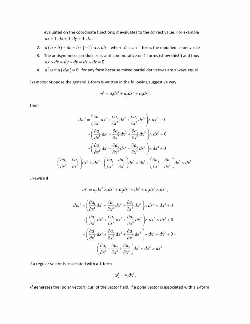
evaluated on the coordinate functions, it evaluates to the correct value. For example 1 0 0dx dx dy dz= ⋅ + ⋅ + ⋅ .
2. ( ) ( )1 id a b da b a db∧ = ∧ + − ∧ where a is an i ‐form, the modified Leibnitz rule
3. The antisymmetric product ∧ is anti‐commutative on 1‐forms (show this!!) and thus 0dx dx dy dy dz dz∧ = ∧ = ∧ =
4. ( )2 0d d dω ω≡ = for any form because mixed partial derivatives are always equal
Examples: Suppose the general 1‐form is written in the following suggestive way
1 1 2 31 2 3 .a dx a dx a dxω = + +
Then
1 1 2 3 11 1 11 2 3
1 2 3 22 2 21 2 3
1 2 3 33 3 31 2 3
3
0
0
0
a a ad dx dx dx dxx x xa a adx dx dx dxx x xa a adx dx dx dxx x x
ax
ω ∂ ∂ ∂⎛ ⎞= + + ∧ +⎜ ⎟∂ ∂ ∂⎝ ⎠∂ ∂ ∂⎛ ⎞+ + + ∧ +⎜ ⎟∂ ∂ ∂⎝ ⎠∂ ∂ ∂⎛ ⎞+ + + ∧ + =⎜ ⎟∂ ∂ ∂⎝ ⎠
∂∂
2 3 3 1 1 232 1 2 12 3 3 1 1 2 .aa a a adx dx dx dx dx dx
x x x x x∂∂ ∂ ∂ ∂⎛ ⎞ ⎛ ⎞ ⎛ ⎞− ∧ + − ∧ + − ∧⎜ ⎟⎜ ⎟ ⎜ ⎟∂ ∂ ∂ ∂ ∂⎝ ⎠⎝ ⎠ ⎝ ⎠
Likewise if
2 2 3 3 1 1 21 2 3 ,a dx dx a dx dx a dx dxω = ∧ + ∧ + ∧
2 1 2 3 2 31 1 11 2 3
1 2 3 3 12 2 21 2 3
1 2 3 1 23 3 31 2 3
31 21 2 3
0
0
0
a a ad dx dx dx dx dxx x xa a adx dx dx dx dxx x xa a adx dx dx dx dxx x x
aa ax x x
ω ∂ ∂ ∂⎛ ⎞= + + ∧ ∧ +⎜ ⎟∂ ∂ ∂⎝ ⎠∂ ∂ ∂⎛ ⎞+ + + ∧ ∧ +⎜ ⎟∂ ∂ ∂⎝ ⎠∂ ∂ ∂⎛ ⎞+ + + ∧ ∧ + =⎜ ⎟∂ ∂ ∂⎝ ⎠
∂∂ ∂⎛ ⎞+ +⎜ ∂ ∂ ∂⎝ ⎠1 2 3dx dx dx∧ ∧⎟
If a regular vector is associated with a 1‐form
1v v i
idxω = ,
d generates the (polar vector!) curl of the vector field. If a polar vector is associated with a 2‐form
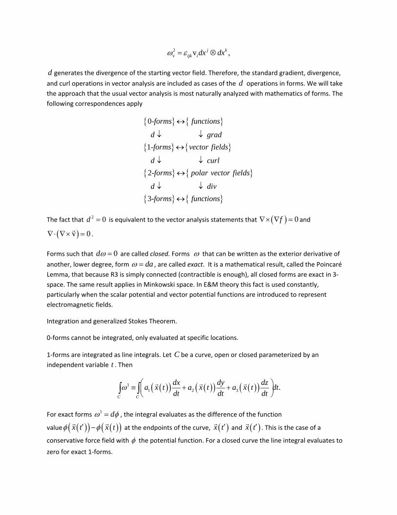
2v v ,j k
ijk idx dxω ε= ⊗
d generates the divergence of the starting vector field. Therefore, the standard gradient, divergence,
and curl operations in vector analysis are included as cases of the d operations in forms. We will take the approach that the usual vector analysis is most naturally analyzed with mathematics of forms. The following correspondences apply
{ } { }
{ } { }
{ } { }
{ } { }
0-
1-
2-
3-
forms functions
d gradforms vector fields
d curlforms polar vector fields
d divforms functions
↔
↓ ↓
↔
↓ ↓
↔
↓ ↓
↔
The fact that 2 0d = is equivalent to the vector analysis statements that ( ) 0f∇× ∇ = and
( )v 0∇⋅ ∇× =r
.
Forms such that 0dω = are called closed. Forms ω that can be written as the exterior derivative of
another, lower degree, form daω = , are called exact. It is a mathematical result, called the Poincaré Lemma, that because R3 is simply connected (contractible is enough), all closed forms are exact in 3‐space. The same result applies in Minkowski space. In E&M theory this fact is used constantly, particularly when the scalar potential and vector potential functions are introduced to represent electromagnetic fields.
Integration and generalized Stokes Theorem.
0‐forms cannot be integrated, only evaluated at specific locations.
1‐forms are integrated as line integrals. Let C be a curve, open or closed parameterized by an independent variable t . Then
( )( ) ( )( ) ( )( )11 2 3 .
C C
dx dy dza x t a x t a x t dtdt dt dt
ω ⎛ ⎞≡ + +⎜ ⎟⎝ ⎠∫ ∫
r r r
For exact forms 1 dω φ= , the integral evaluates as the difference of the function
value ( )( ) ( )( )x t x tφ φ′ −r r
at the endpoints of the curve, ( )x t′r and ( )x t′r
. This is the case of a
conservative force field with φ the potential function. For a closed curve the line integral evaluates to
zero for exact 1‐forms.
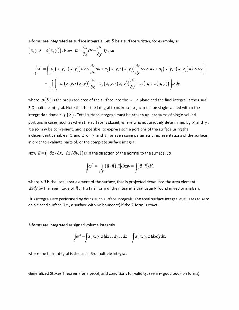
2‐forms are integrated as surface integrals. Let S be a surface written, for example, as
( )( ), , ,x y z s x y= . Now s sdz dx dyx y∂ ∂
= +∂ ∂
, so
( )( ) ( )( ) ( )( )
( )( ) ( )( ) ( )( )
21 2 3
1 2 3( )
, , , , , , , , ,
, , , , , , , , ,
S S
p S
s sa x y s x y dy dx a x y s x y dy dx a x y s x y dx dyx y
s sa x y s x y a x y s x y a x y s x y dxdyx y
ω⎛ ⎞∂ ∂
≡ ∧ + ∧ + ∧⎜ ⎟∂ ∂⎝ ⎠⎛ ⎞∂ ∂
= − − +⎜ ⎟∂ ∂⎝ ⎠
∫ ∫
∫
where ( )p S is the projected area of the surface into the x ‐ y plane and the final integral is the usual
2‐D multiple integral. Note that for the integral to make sense, s must be single‐valued within the
integration domain ( )p S . Total surface integrals must be broken up into sums of single‐valued
portions in cases, such as when the surface is closed, where z is not uniquely determined by x and y .
It also may be convenient, and is possible, to express some portions of the surface using the independent variables x and z or y and z , or even using parametric representations of the surface,
in order to evaluate parts of, or the complete surface integral.
Now ( )/ , / ,1n z x z y= −∂ ∂ −∂ ∂r
is in the direction of the normal to the surface. So
( ) ( )2
( )
ˆ ˆS p S S
a n n dxdy a n dAω = ⋅ = ⋅∫ ∫ ∫r r r
where dA is the local area element of the surface, that is projected down into the area element
dxdy by the magnitude of nr . This final form of the integral is that usually found in vector analysis.
Flux integrals are performed by doing such surface integrals. The total surface integral evaluates to zero on a closed surface (i.e., a surface with no boundary) if the 2‐form is exact.
3‐forms are integrated as signed volume integrals
( ) ( )3 , , , , .V V V
a x y z dx dy dz a x y z dxdydzω ≡ ∧ ∧ =∫ ∫ ∫
where the final integral is the usual 3‐d multiple integral.
Generalized Stokes Theorem (for a proof, and conditions for validity, see any good book on forms)
If M is a manifold and ω a form that exists throughout the manifold, then
M M
dω ω∂
=∫ ∫
where M∂ is the boundary of M . We will be applying this theorem to various regions of 3‐space and Minkowski space, although it works for, and inside of much more general manifolds. Within it are the main theorems of vector analysis.
Fundamental Theorem of Calculus: Applied to [a,b] in R . If fω =
[ ]( ) ( )
,
b
aa b
df dx f f b f adx
= = −∫
Green’s Theorem: Applied to a simply connected region R of 2R . If Pdx Qdyω = +
( )( )
/ .R R p R
Q P dxdy Pdx Qdy P Qdy dx dxx y ∂ ∂
⎛ ⎞∂ ∂− = + = +⎜ ⎟∂ ∂⎝ ⎠
∫ ∫ ∫
The second equality applies in the case that ( )y x is the monotonic, and single‐valued equation for the
boundary curve in terms of the independent variable x . Note that if 0dω = , i.e. the form is exact, the line integrals are always independent of path, as above.
Stoke’s Theorem: Applied to a simply connected surface in 3R . If Pdx Qdy Rdzω = + + and
( ) ( ) ( ) ( )( ), , , , , , , , , ,A x y z P x y z Q x y z R x y z≡r
( ) ˆ
.
.
S S
S S
R Q P R Q PA ndS dy dz dz dx dx dyy z z x x y
Pdx Qdy Rdz A dr∂ ∂
⎛ ⎞ ⎛ ⎞∂ ∂ ∂ ∂ ∂ ∂⎛ ⎞∇× ⋅ = − ∧ + − ∧ + − ∧⎜ ⎟ ⎜ ⎟⎜ ⎟∂ ∂ ∂ ∂ ∂ ∂⎝ ⎠⎝ ⎠ ⎝ ⎠
= + + = ⋅
∫ ∫
∫ ∫
r
r r
Note that if ω is exact, A φ= ∇r
for some function, and we again have independence of path. In this
case all surface integrals vanish, consistent with the usual vector analysis result that 0φ∇×∇ = . A non‐
zero line integral requires a curl to be generated.
Divergence, or Gauss’s Theorem: Applied to a simply connected volume in 3R . If
Pdy dz Qdz dx Rdx dyω = ∧ + ∧ + ∧ , ( ) ( ) ( ) ( )( ), , , , , , , , , ,A x y z P x y z Q x y z R x y z≡r
( ) ˆ .V V V V
P Q RA dV dx dy dz Pdy dz Qdz dx Rdx dy A ndSx y z ∂ ∂
⎛ ⎞∂ ∂ ∂∇ ⋅ = + + ∧ ∧ = ∧ + ∧ + ∧ = ⋅⎜ ⎟∂ ∂ ∂⎝ ⎠
∫ ∫ ∫ ∫r r
If ω is exact, i.e., 0A∇⋅ =r
, then suppose c is a closed curve in boundary V. The flux integral through the curve is independent of the bounding surface used to evaluate the flux . This is a 2‐dimensional result analogous to the path independent integrals for 1‐forms. This result has implications for magnetic
field lines, which always must close as 0B∇⋅ =r
.
Extra formulas in Jackson: Let 0Q R= = in the Divergence Theorem, and P ψ= . Then
( )ˆ ˆ .V V V
dx dy dz dy dz n x dSxψ ψ ψ
∂ ∂
∂∧ ∧ = ∧ = ⋅
∂∫ ∫ ∫
Likewise,
( ) ( )ˆ ˆ ˆ ˆ and .V V V V V V
dx dy dz dz dx n y dS dx dy dz dx dy n z dSy zψ ψψ ψ ψ ψ
∂ ∂ ∂ ∂
∂ ∂∧ ∧ = ∧ = ⋅ ∧ ∧ = ∧ = ⋅
∂ ∂∫ ∫ ∫ ∫ ∫ ∫
Summing with the constant unit vectors gives
ˆV V
dxdydz ndSψ ψ∂
∇ =∫ ∫
Using formulas like
( )ˆ ˆyy y
V V V
Adx dy dz A dz dx A n x dS
x ∂ ∂
∂∧ ∧ = ∧ = ⋅
∂∫ ∫ ∫
One readily verifies that
ˆ .V V
Adxdydz n AdS∂
∇× = ×∫ ∫r r
Following a similar analysis, let 0Q R= = in Stokes Theorem, and P ψ= . Then
( ) ( )ˆ ˆ ˆ ˆ .S S S
n y dS n z dS dz dx dx dy dxz y z yψ ψ ψ ψ ψ
∂
∂ ∂ ∂ ∂⋅ − ⋅ = ∧ − ∧ =
∂ ∂ ∂ ∂∫ ∫ ∫
Likewise,
( ) ( )ˆ ˆ ˆ ˆ , and S S
n x dS n z dS dyz xψ ψ ψ
∂
∂ ∂− ⋅ + ⋅ =∂ ∂∫ ∫
( ) ( )ˆ ˆ ˆ ˆ .S S
n x dS n y dS dzy xψ ψ ψ
∂
∂ ∂⋅ − ⋅ =
∂ ∂∫ ∫
Summing, with unit vectors as before yields
ˆ .S S
n dS drψ ψ∂
×∇ =∫ ∫r
This document provides a condensed summary of the mathematics of forms that we will need going forward. We will be expressing the electromagnetic field quantities in terms of forms; applying these methods will allow one to derive fairly deep results more quickly and rigorously than is possible using more standard vector analysis. One motivation for this adoption is the idea that “forms are made to be integrated”. 1‐forms are appropriately evaluated as line integrals, 2‐forms are evaluated as surface integrals, and 3‐forms as volume integrals. One can work this backwards. If one has a physical quantity best evaluated with a line integral, a 1‐form is the appropriate description. Flux integrals must be completed with a 2‐form. Quantities that involve volume densities, for example the charge density, are best represented as 3‐forms.


![Exercise 5–1 Ex: 5.1 Similarly, V 1 V results in ...ece.gmu.edu/~qli/ECE333/Chapter 05 ISM.pdfSEDRA-ISM: “E-CH05 ... = 1.23 V Ex: 5.17 v DSmin = v GS +|V t| ... × 2[1 −( )]2](https://static.fdocument.org/doc/165x107/5adf970e7f8b9a1c248c32ec/exercise-51-ex-51-similarly-v-1-v-results-in-ecegmueduqliece333chapter.jpg)