STAT 200C: High-dimensional Statistics

Arash A. Amini

May 30, 2018

1 / 57

Table of Contents

1 Sparse linear modelsBasis Pursuit and restricted null space propertySufficient conditions for RNS

2 / 57

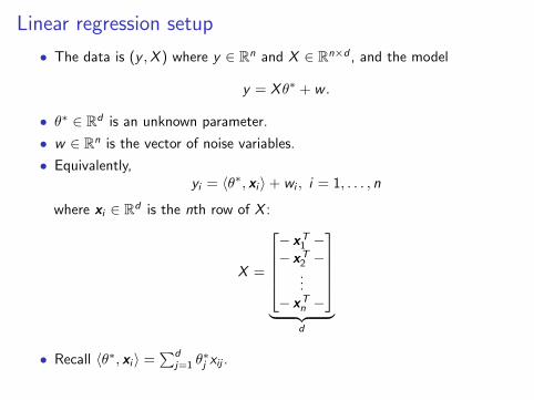
Linear regression setup

• The data is (y ,X ) where y ∈ Rn and X ∈ Rn×d , and the model

y = Xθ∗ + w .

• θ∗ ∈ Rd is an unknown parameter.

• w ∈ Rn is the vector of noise variables.

• Equivalently,yi = 〈θ∗, xi 〉+ wi , i = 1, . . . , n

where xi ∈ Rd is the nth row of X :

X =

− xT

1 −− xT

2 −...

− xTn −

︸ ︷︷ ︸

d

• Recall 〈θ∗, xi 〉 =∑d

j=1 θ∗j xij .

3 / 57

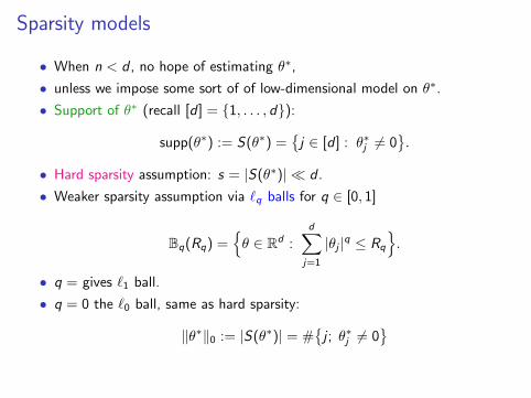
Sparsity models

• When n < d , no hope of estimating θ∗,

• unless we impose some sort of of low-dimensional model on θ∗.

• Support of θ∗ (recall [d ] = {1, . . . , d}):

supp(θ∗) := S(θ∗) ={j ∈ [d ] : θ∗j 6= 0

}.

• Hard sparsity assumption: s = |S(θ∗)| � d .

• Weaker sparsity assumption via `q balls for q ∈ [0, 1]

Bq(Rq) ={θ ∈ Rd :

d∑j=1

|θj |q ≤ Rq

}.

• q = gives `1 ball.

• q = 0 the `0 ball, same as hard sparsity:

‖θ∗‖0 := |S(θ∗)| = #{j ; θ∗j 6= 0

}4 / 57

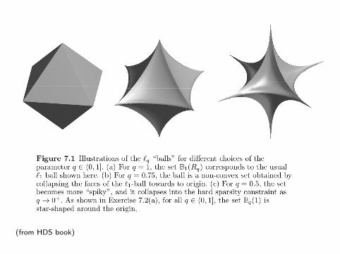
(from HDS book)

5 / 57

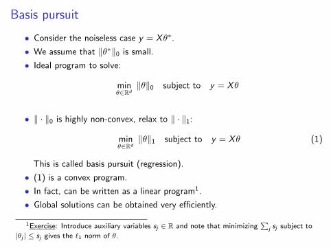
Basis pursuit

• Consider the noiseless case y = Xθ∗.

• We assume that ‖θ∗‖0 is small.

• Ideal program to solve:

minθ∈Rd

‖θ‖0 subject to y = Xθ

• ‖ · ‖0 is highly non-convex, relax to ‖ · ‖1:

minθ∈Rd

‖θ‖1 subject to y = Xθ (1)

This is called basis pursuit (regression).

• (1) is a convex program.

• In fact, can be written as a linear program1.

• Global solutions can be obtained very efficiently.

1Exercise: Introduce auxiliary variables sj ∈ R and note that minimizing∑

j sj subject to

|θj | ≤ sj gives the `1 norm of θ.6 / 57

Table of Contents

1 Sparse linear modelsBasis Pursuit and restricted null space propertySufficient conditions for RNS

7 / 57

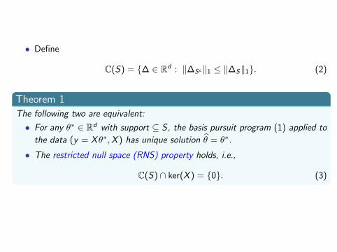
• Define

C(S) = {∆ ∈ Rd : ‖∆Sc‖1 ≤ ‖∆S‖1}. (2)

Theorem 1The following two are equivalent:

• For any θ∗ ∈ Rd with support ⊆ S , the basis pursuit program (1) applied to

the data (y = Xθ∗,X ) has unique solution θ = θ∗.

• The restricted null space (RNS) property holds, i.e.,

C(S) ∩ ker(X ) = {0}. (3)

8 / 57

Proof

• Consider the tangent cone to the `1 ball (of radius ‖θ∗‖1) at θ∗:

T(θ∗) = {∆ ∈ Rd : ‖θ∗ + t∆‖1 ≤ ‖θ∗‖1, for some t > 0.}

i.e., the set of descent directions for `1 norm at point θ∗.

• Feasible set is θ∗ + ker(X ), i.e.

• ker(X ) is the set of feasible directions ∆ = θ − θ∗.• Hence, there is a minimizer other than θ∗ if and only if

T(θ∗) ∩ ker(X ) 6= {0} (4)

• It is enough to show that

C(S) =⋃

θ∗∈Rd : supp(θ∗)⊆ST(θ∗).

9 / 57

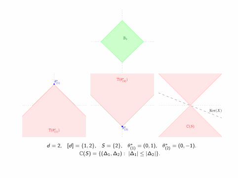
B1

•θ∗(1)

T(θ∗(1))•θ∗(2)

T(θ∗(2))

Ker(X)

C(S)

d = 2, [d ] = {1, 2}, S = {2}, θ∗(1)

= (0, 1), θ∗(2)

= (0,−1).

C(S) = {(∆1,∆2) : |∆1| ≤ |∆2|}.

10 / 57

• It is enough to show that

C(S) =⋃

θ∗∈Rd : supp(θ∗)⊆ST(θ∗) (5)

• We have ∆ ∈ T1(θ∗) iff2

‖∆Sc‖1 ≤ ‖θ∗S‖1 − ‖θ∗S + ∆S‖1

• We have ∆ ∈ T1(θ∗) for some θ∗ ∈ Rd s.t. supp(θ∗) ⊂ S iff

‖∆Sc‖1 ≤ supθ∗S∈Rd

[‖θ∗S‖1 − ‖θ∗S + ∆S‖1

]= ‖∆S‖1

2Let T1(θ∗) be the subset of T(θ∗) where t = 1, and argue that w.l.o.g. we can work thissubset.

11 / 57

Table of Contents

1 Sparse linear modelsBasis Pursuit and restricted null space propertySufficient conditions for RNS

12 / 57

Sufficient conditions for restricted nullspace

• [d ] := {1, . . . , d}• For a matrix X ∈ Rd , let Xj be its jth column (for j ∈ [d ]).

• The pairwise incoherence of X is defined as

δPW(X ) := maxi, j∈[d ]

∣∣∣ 〈Xi ,Xj〉n

− 1{i = j}∣∣∣

• Alternative form: XTX is the Gram matrix of X ,

• (XTX )ij = 〈Xi ,Xj〉.

δPW(X ) := ‖XTX

n− Ip‖∞

where ‖ · ‖∞ is the vector `∞ norm of the matrix.

13 / 57

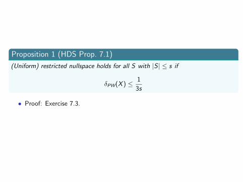
Proposition 1 (HDS Prop. 7.1)

(Uniform) restricted nullspace holds for all S with |S | ≤ s if

δPW(X ) ≤ 1

3s

• Proof: Exercise 7.3.

14 / 57

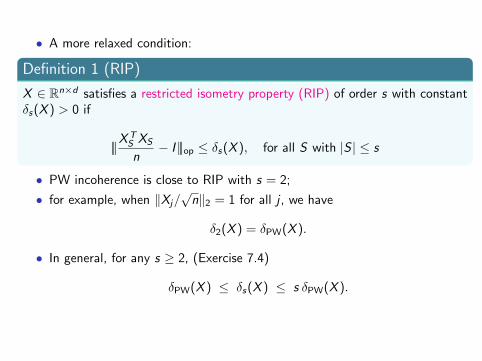
• A more relaxed condition:

Definition 1 (RIP)

X ∈ Rn×d satisfies a restricted isometry property (RIP) of order s with constantδs(X ) > 0 if

|||XTS XS

n− I |||op ≤ δs(X ), for all S with |S | ≤ s

• PW incoherence is close to RIP with s = 2;

• for example, when ‖Xj/√n‖2 = 1 for all j , we have

δ2(X ) = δPW(X ).

• In general, for any s ≥ 2, (Exercise 7.4)

δPW(X ) ≤ δs(X ) ≤ s δPW(X ).

15 / 57

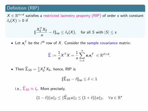
Definition (RIP)

X ∈ Rn×d satisfies a restricted isometry property (RIP) of order s with constantδs(X ) > 0 if

|||XTS XS

n− I |||op ≤ δs(X ), for all S with |S | ≤ s

• Let xTi be the i th row of X . Consider the sample covariance matrix:

Σ :=1

nXTX =

1

n

n∑i=1

xixTi ∈ Rd×d .

• Then ΣSS = 1nX

TS XS , hence, RIP is

|||ΣSS − I |||op ≤ δ < 1

i.e., ΣSS ≈ Is . More precisely,

(1− δ)‖u‖2 ≤ ‖ΣSSu‖2 ≤ (1 + δ)‖u‖2, ∀u ∈ Rs

16 / 57

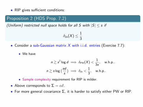
• RIP gives sufficient conditions:

Proposition 2 (HDS Prop. 7.2)

(Uniform) restricted null space holds for all S with |S | ≤ s if

δ2s(X ) ≤ 1

3

• Consider a sub-Gaussian matrix X with i.i.d. entries (Exercise 7.7):

• We have

n & s2 log d =⇒ δPW(X ) <1

3s, w.h.p..

n & s log(eds

)=⇒ δ2s <

1

3, w.h.p..

• Sample complexity requirement for RIP is milder.

• Above corresponds to Σ = αI .

• For more general covariance Σ, it is harder to satisfy either PW or RIP.

17 / 57

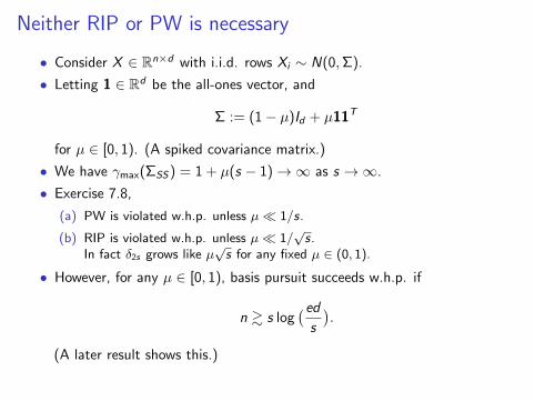
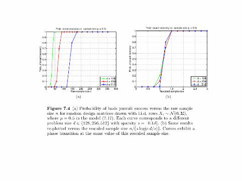
Neither RIP or PW is necessary

• Consider X ∈ Rn×d with i.i.d. rows Xi ∼ N(0,Σ).

• Letting 1 ∈ Rd be the all-ones vector, and

Σ := (1− µ)Id + µ11T

for µ ∈ [0, 1). (A spiked covariance matrix.)

• We have γmax(ΣSS) = 1 + µ(s − 1)→∞ as s →∞.

• Exercise 7.8,

(a) PW is violated w.h.p. unless µ� 1/s.

(b) RIP is violated w.h.p. unless µ� 1/√s.

In fact δ2s grows like µ√s for any fixed µ ∈ (0, 1).

• However, for any µ ∈ [0, 1), basis pursuit succeeds w.h.p. if

n & s log(eds

).

(A later result shows this.)

18 / 57

19 / 57

Noisy sparse regression

• A very popular estimator is the `1-regularized least-squares:

θ ∈ argminθ∈Rd

[ 1

2n‖y − Xθ‖2

2 + λ‖θ‖1

](6)

• The idea: minimizing `1 norm leads to sparse solutions.

• (6) is a convex program; global solution can be obtained efficiently.

• Other options: constrained form of lasso

min‖θ‖1≤R

1

2n‖y − Xθ‖2

2 (7)

and relaxed basis persuit

minθ∈Rd‖θ‖1 s.t.

1

2n‖y − Xθ‖2

2 ≤ b2 (8)

20 / 57

• For a constant α ≥ 1,

Cα(S) :={

∆ ∈ Rd | ‖∆Sc‖1 ≤ α‖∆S‖1

}.

• A strengthening of RNS is:

Definition 2 (RE condition)

A matrix X satisfies the restricted eigenvalue (RE) condition over S withparameters (κ, α) if

1

n‖X∆‖2

2 ≥ κ‖∆‖22 for all ∆ ∈ Cα(S).

• Intuition: θ minimizes L(θ) := 12n‖Xθ − y‖2.

• Ideally, δL := L(θ)− L(θ∗) is small.

• Want to translate deviation in loss to deviations in parameter θ − θ∗.• Controlled by the curvature of the loss, captured by the Hessian

∇2L(θ) =1

nXTX .

21 / 57

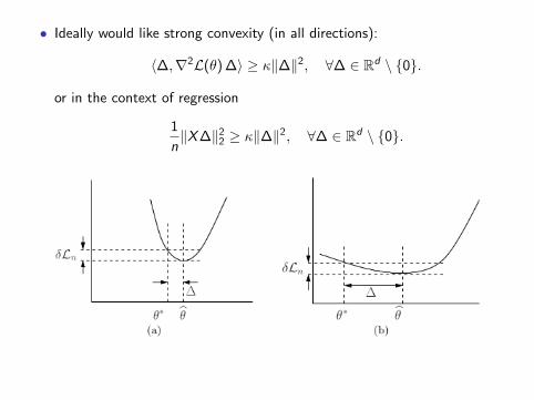
• Ideally would like strong convexity (in all directions):

〈∆,∇2L(θ) ∆〉 ≥ κ‖∆‖2, ∀∆ ∈ Rd \ {0}.

or in the context of regression

1

n‖X∆‖2

2 ≥ κ‖∆‖2, ∀∆ ∈ Rd \ {0}.

22 / 57

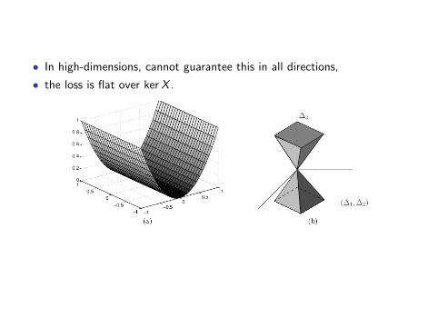
• In high-dimensions, cannot guarantee this in all directions,

• the loss is flat over kerX .

23 / 57

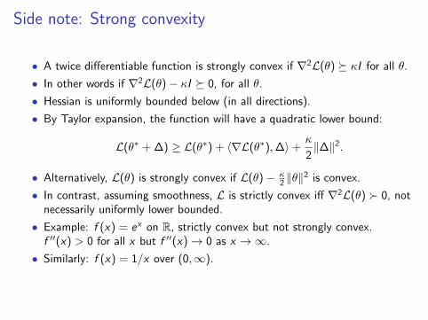
Side note: Strong convexity

• A twice differentiable function is strongly convex if ∇2L(θ) � κI for all θ.

• In other words if ∇2L(θ)− κI � 0, for all θ.

• Hessian is uniformly bounded below (in all directions).

• By Taylor expansion, the function will have a quadratic lower bound:

L(θ∗ + ∆) ≥ L(θ∗) + 〈∇L(θ∗),∆〉+κ

2‖∆‖2.

• Alternatively, L(θ) is strongly convex if L(θ)− κ2 ‖θ‖2 is convex.

• In contrast, assuming smoothness, L is strictly convex iff ∇2L(θ) � 0, notnecessarily uniformly lower bounded.

• Example: f (x) = ex on R, strictly convex but not strongly convex.f ′′(x) > 0 for all x but f ′′(x)→ 0 as x →∞.

• Similarly: f (x) = 1/x over (0,∞).

24 / 57

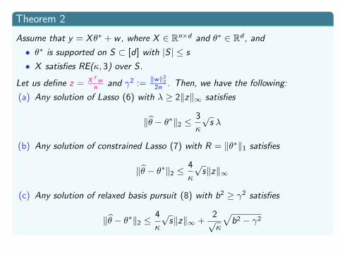
Theorem 2

Assume that y = Xθ∗ + w , where X ∈ Rn×d and θ∗ ∈ Rd , and

• θ∗ is supported on S ⊂ [d ] with |S | ≤ s

• X satisfies RE(κ, 3) over S .

Let us define z = XTwn and γ2 :=

‖w‖22

2n . Then, we have the following:

(a) Any solution of Lasso (6) with λ ≥ 2‖z‖∞ satisfies

‖θ − θ∗‖2 ≤3

κ

√s λ

(b) Any solution of constrained Lasso (7) with R = ‖θ∗‖1 satisfies

‖θ − θ∗‖2 ≤4

κ

√s‖z‖∞

(c) Any solution of relaxed basis pursuit (8) with b2 ≥ γ2 satisfies

‖θ − θ∗‖2 ≤4

κ

√s‖z‖∞ +

2√κ

√b2 − γ2

25 / 57

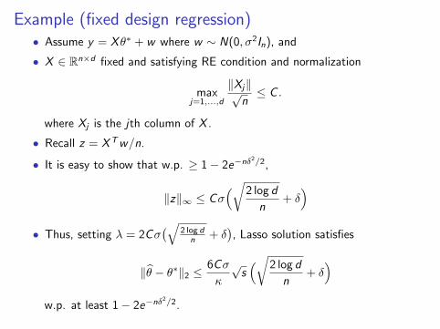
Example (fixed design regression)• Assume y = Xθ∗ + w where w ∼ N(0, σ2In), and

• X ∈ Rn×d fixed and satisfying RE condition and normalization

maxj=1,...,d

‖Xj‖√n≤ C .

where Xj is the jth column of X .

• Recall z = XTw/n.

• It is easy to show that w.p. ≥ 1− 2e−nδ2/2,

‖z‖∞ ≤ Cσ(√2 log d

n+ δ)

• Thus, setting λ = 2Cσ(√

2 log dn + δ

), Lasso solution satisfies

‖θ − θ∗‖2 ≤6Cσ

κ

√s(√2 log d

n+ δ)

w.p. at least 1− 2e−nδ2/2.

26 / 57

• Taking δ =√

2 log /n, we have

‖θ − θ∗‖2 . σ

√s log d

n

w.h.p. (i.e., ≥ 1− 2d−1).

• This is the typical high-dimensional scaling in sparse problems.

• Had we known the support S in advance, our rate would be (w.h.p.)

‖θ − θ∗‖2 . σ

√s

n.

• The log d factor is the price for not knowing the support;

• roughly the price for searching over(ds

)≤ d s collection of candidate

supports.

27 / 57

Proof of Theorem 2

• Let us simplify the loss L(θ) := 12n‖Xθ − y‖2.

• Setting ∆ = θ − θ∗,

L(θ) =1

2n‖X (θ − θ∗)− w‖2

=1

2n‖X∆− w‖2

=1

2n‖X∆‖2 − 1

n〈X∆,w〉+ const.

=1

2n‖X∆‖2 − 1

n〈∆,XTw〉+ const.

=1

2n‖X∆‖2 − 〈∆, z〉+ const.

where z = XTw/n. Hence,

L(θ)− L(θ∗) =1

2n‖X∆‖2 − 〈∆, z〉. (9)

• Exercise: Show that (9) is the Taylor expansion of L around θ∗.

28 / 57

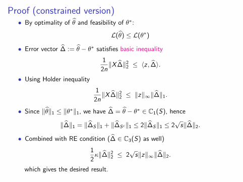
Proof (constrained version)• By optimality of θ and feasibility of θ∗:

L(θ) ≤ L(θ∗)

• Error vector ∆ := θ − θ∗ satisfies basic inequality

1

2n‖X ∆‖2

2 ≤ 〈z , ∆〉.

• Using Holder inequality

1

2n‖X ∆‖2

2 ≤ ‖z‖∞‖∆‖1.

• Since ‖θ‖1 ≤ ‖θ∗‖1, we have ∆ = θ − θ∗ ∈ C1(S), hence

‖∆‖1 = ‖∆S‖1 + ‖∆Sc‖1 ≤ 2‖∆S‖1 ≤ 2√s‖∆‖2.

• Combined with RE condition (∆ ∈ C3(S) as well)

1

2κ‖∆‖2

2 ≤ 2√s‖z‖∞‖∆‖2.

which gives the desired result.

29 / 57

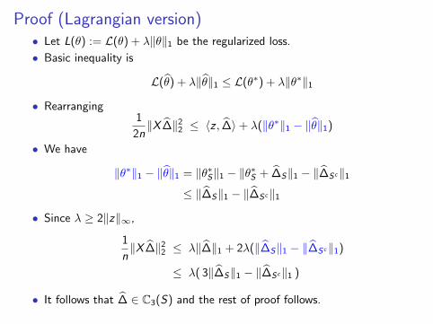
Proof (Lagrangian version)• Let L(θ) := L(θ) + λ‖θ‖1 be the regularized loss.

• Basic inequality is

L(θ) + λ‖θ‖1 ≤ L(θ∗) + λ‖θ∗‖1

• Rearranging1

2n‖X ∆‖2

2 ≤ 〈z , ∆〉+ λ(‖θ∗‖1 − ‖θ‖1)

• We have

‖θ∗‖1 − ‖θ‖1 = ‖θ∗S‖1 − ‖θ∗S + ∆S‖1 − ‖∆Sc‖1

≤ ‖∆S‖1 − ‖∆Sc‖1

• Since λ ≥ 2‖z‖∞,

1

n‖X ∆‖2

2 ≤ λ‖∆‖1 + 2λ(‖∆S‖1 − ‖∆Sc‖1)

≤ λ( 3‖∆S‖1 − ‖∆Sc‖1 )

• It follows that ∆ ∈ C3(S) and the rest of proof follows.

30 / 57

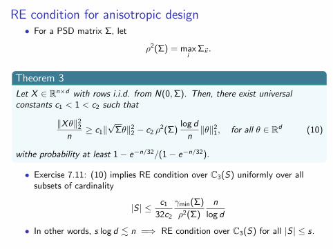
RE condition for anisotropic design• For a PSD matrix Σ, let

ρ2(Σ) = maxi

Σii .

Theorem 3

Let X ∈ Rn×d with rows i.i.d. from N(0,Σ). Then, there exist universalconstants c1 < 1 < c2 such that

‖Xθ‖22

n≥ c1‖

√Σθ‖2

2 − c2 ρ2(Σ)

log d

n‖θ‖2

1, for all θ ∈ Rd (10)

withe probability at least 1− e−n/32/(1− e−n/32).

• Exercise 7.11: (10) implies RE condition over C3(S) uniformly over allsubsets of cardinality

|S | ≤ c1

32c2

γmin(Σ)

ρ2(Σ)

n

log d

• In other words, s log d . n =⇒ RE condition over C3(S) for all |S | ≤ s.

31 / 57

Examples

• Toeplitz family: Σij = ν|i−j|,

ρ2(Σ) = 1, γmin(Σ) ≥ (1− ν)2 > 0

• Spiked model: Σ := (1− µ)Id + µ11T ,

ρ2(Σ) = 1, γmin(Σ) = 1− µ

• For future applications, note that (10) implies

‖Xθ‖22

n≥ α1‖θ‖2

2 − α2‖θ‖21, ∀θ ∈ Rd .

where α1 = c1γmin(Σ) and α2 = c2ρ2(Σ)

log d

n.

32 / 57

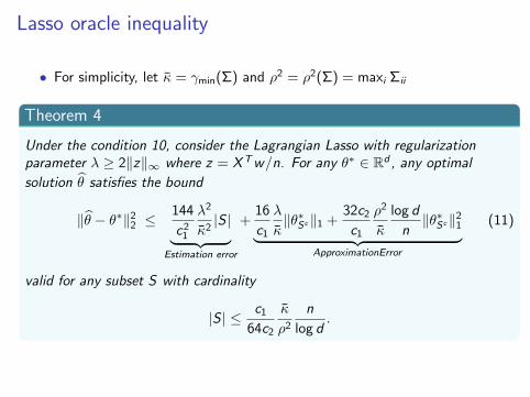
Lasso oracle inequality

• For simplicity, let κ = γmin(Σ) and ρ2 = ρ2(Σ) = maxi Σii

Theorem 4

Under the condition 10, consider the Lagrangian Lasso with regularizationparameter λ ≥ 2‖z‖∞ where z = XTw/n. For any θ∗ ∈ Rd , any optimal

solution θ satisfies the bound

‖θ − θ∗‖22 ≤

144

c21

λ2

κ2|S |︸ ︷︷ ︸

Estimation error

+16

c1

λ

κ‖θ∗Sc‖1 +

32c2

c1

ρ2

κ

log d

n‖θ∗Sc‖2

1︸ ︷︷ ︸ApproximationError

(11)

valid for any subset S with cardinality

|S | ≤ c1

64c2

κ

ρ2

n

log d.

33 / 57

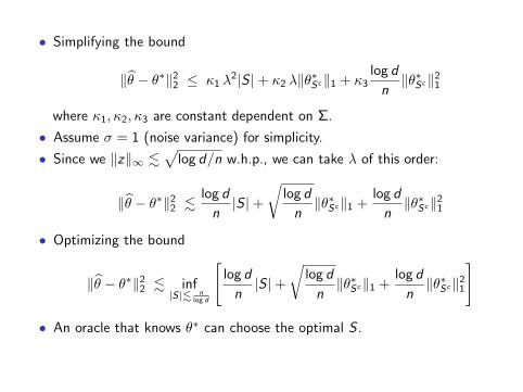
• Simplifying the bound

‖θ − θ∗‖22 ≤ κ1 λ

2|S |+ κ2 λ‖θ∗Sc‖1 + κ3log d

n‖θ∗Sc‖2

1

where κ1, κ2, κ3 are constant dependent on Σ.

• Assume σ = 1 (noise variance) for simplicity.

• Since we ‖z‖∞ .√

log d/n w.h.p., we can take λ of this order:

‖θ − θ∗‖22 .

log d

n|S |+

√log d

n‖θ∗Sc‖1 +

log d

n‖θ∗Sc‖2

1

• Optimizing the bound

‖θ − θ∗‖22 . inf

|S|. nlog d

[log d

n|S |+

√log d

n‖θ∗Sc‖1 +

log d

n‖θ∗Sc‖2

1

]

• An oracle that knows θ∗ can choose the optimal S .

34 / 57

Example: `q-ball sparsity

• Assume that θ∗ ∈ Bq, i.e.,∑d

j=1 |θ∗j |q ≤ 1, for some q ∈ [0, 1].

• Then, assuming σ2 = 1, we have the rate (Exercise 7.12)

‖θ − θ∗‖22 .

( log d

n

)1−q/2

.

Sketch:

• Trick: take S = {i : |θ∗i | > τ} and find a good threshold τ later.

• Show that ‖θ∗Sc‖1 ≤ τ 1−q and |S | ≤ τ−q.

• The bound would be of the form (ε :=√

log d/n)

ε2τ−q + ετ 1−q + (ετ 1−q)2.

• Ignore the last term (assuming ετ 1−q ≤ 1, it is not dominant),

35 / 57

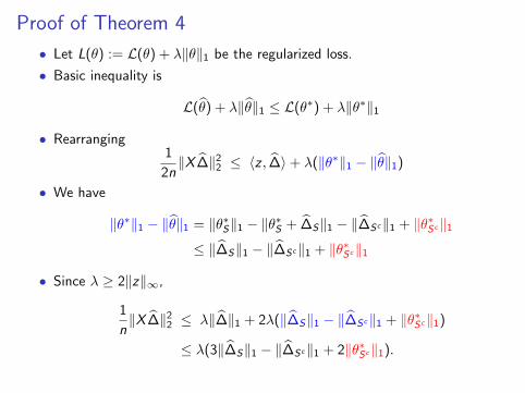
Proof of Theorem 4

• Let L(θ) := L(θ) + λ‖θ‖1 be the regularized loss.

• Basic inequality is

L(θ) + λ‖θ‖1 ≤ L(θ∗) + λ‖θ∗‖1

• Rearranging1

2n‖X ∆‖2

2 ≤ 〈z , ∆〉+ λ(‖θ∗‖1 − ‖θ‖1)

• We have

‖θ∗‖1 − ‖θ‖1 = ‖θ∗S‖1 − ‖θ∗S + ∆S‖1 − ‖∆Sc‖1 + ‖θ∗Sc‖1

≤ ‖∆S‖1 − ‖∆Sc‖1 + ‖θ∗Sc‖1

• Since λ ≥ 2‖z‖∞,

1

n‖X ∆‖2

2 ≤ λ‖∆‖1 + 2λ(‖∆S‖1 − ‖∆Sc‖1 + ‖θ∗Sc‖1)

≤ λ(3‖∆S‖1 − ‖∆Sc‖1 + 2‖θ∗Sc‖1).

36 / 57

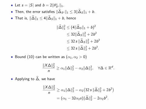
• Let s = |S | and b = 2‖θ∗Sc‖1.

• Then, the error satisfies ‖∆Sc‖1 ≤ 3‖∆S‖1 + b.

• That is, ‖∆‖1 ≤ 4‖∆S‖1 + b, hence

‖∆‖21 ≤ (4‖∆S‖1 + b)2

≤ 32‖∆S‖21 + 2b2

≤ 32 s ‖∆S‖22 + 2b2

≤ 32 s ‖∆‖22 + 2b2.

• Bound (10) can be written as (α1, α2 > 0)

‖X∆‖22

n≥ α1‖∆‖2

2 − α2‖∆‖21, ∀∆ ∈ Rd .

• Applying to ∆, we have

‖X∆‖22

n≥ α1‖∆‖2

2 − α2

(32 s ‖∆‖2

2 + 2b2)

= (α1 − 32α2s)‖∆‖22 − 2α2b

2.

37 / 57

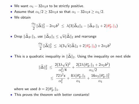
• We want α1 − 32α2s to be strictly positive.

• Assume that α1/2 ≥ 32α2s so that α1 − 32α2s ≥ α1/2.

• We obtain

α1

2‖∆‖2

2 − 2α2b2 ≤ λ(3‖∆S‖1 − ‖∆Sc‖1 + 2‖θ∗Sc‖1)

• Drop ‖∆Sc‖1, use ‖∆S‖1 ≤√s‖∆‖2 and rearrange

α1

2‖∆‖2

2 ≤ λ(3√s‖∆‖2 + 2‖θ∗Sc‖1) + 2α2b

2

• This is a quadratic inequality in ‖∆‖2. Using the inequality on next slide

‖∆‖22 ≤

2(3λ√s)2

α21/4

+2(2λ‖θ∗Sc‖1 + 2α2b

2)

α1/2

≤ 72λ2s

α21

+8λ‖θ∗Sc‖1

α1+

16α2‖θ∗Sc‖21

α1

where we used b = 2‖θ∗Sc‖1.

• This proves the theorem with better constants!

38 / 57

• In general, ax2 ≤ bx + c and x ≥ 0 imply

x ≤ b

a+

√c

a

• which itself implies

x2 ≤ 2b2

a2+

2c

a.

39 / 57

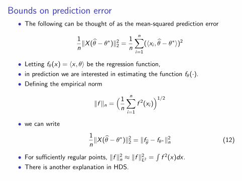
Bounds on prediction error

• The following can be thought of as the mean-squared prediction error

1

n‖X (θ − θ∗)‖2

2 =1

n

n∑i=1

(〈xi , θ − θ∗〉)2

• Letting fθ(x) = 〈x , θ〉 be the regression function,

• in prediction we are interested in estimating the function fθ(·).

• Defining the empirical norm

‖f ‖n =(1

n

n∑i=1

f 2(xi ))1/2

• we can write

1

n‖X (θ − θ∗)‖2

2 = ‖fθ − fθ∗‖2n (12)

• For sufficiently regular points, ‖f ‖2n ≈ ‖f ‖2

L2 =∫f 2(x)dx .

• There is another explanation in HDS.

40 / 57

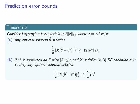
Prediction error bounds

Theorem 5

Consider Lagrangian lasso with λ ≥ 2‖z‖∞ where z = XTw/n:

(a) Any optimal solution θ satisfies

1

n‖X (θ − θ∗)‖2

2 ≤ 12‖θ∗‖1λ

(b) If θ∗ is supported on S with |S | ≤ s and X satisfies (κ, 3)-RE condition overS , they any optimal solution satisfies

1

n‖X (θ − θ∗)‖2

2 ≤9

κsλ2

41 / 57

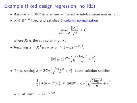
Example (fixed design regression, no RE)

• Assume y = Xθ∗ + w where w has iid σ-sub-Gaussian entries, and

• X ∈ Rn×d fixed and satisfies C -column normalization

maxj=1,...,d

‖Xj‖√n≤ C .

where Xj is the jth column of X .

• Recalling z = XTw/n, w.p. ≥ 1− 2e−nδ2/2,

‖z‖∞ ≤ Cσ(√2 log d

n+ δ)

• Thus, setting λ = 2Cσ(√

2 log dn + δ

), Lasso solution satisfies

1

n‖X (θ − θ∗)‖2

2 ≤ 24‖θ∗‖1Cσ(√2 log d

n+ δ)

w.p. at least 1− 2e−nδ2/2.

42 / 57

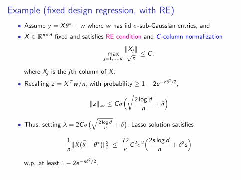
Example (fixed design regression, with RE)

• Assume y = Xθ∗ + w where w has iid σ-sub-Gaussian entries, and

• X ∈ Rn×d fixed and satisfies RE condition and C -column normalization

maxj=1,...,d

‖Xj‖√n≤ C .

where Xj is the jth column of X .

• Recalling z = XTw/n, with probability ≥ 1− 2e−nδ2/2,

‖z‖∞ ≤ Cσ(√2 log d

n+ δ)

• Thus, setting λ = 2Cσ(√

2 log dn + δ

), Lasso solution satisfies

1

n‖X (θ − θ∗)‖2

2 ≤72

κC 2σ2

(2s log d

n+ δ2s

)w.p. at least 1− 2e−nδ

2/2.

43 / 57

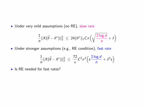
• Under very mild assumptions (no RE), slow rate

1

n‖X (θ − θ∗)‖2

2 ≤ 24‖θ∗‖1Cσ(√2 log d

n+ δ)

• Under stronger assumptions (e.g., RE condition), fast rate

1

n‖X (θ − θ∗)‖2

2 ≤72

κC 2σ2

(s

2 log d

n+ δ2s

)• Is RE needed for fast rates?

44 / 57

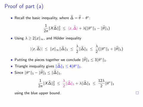
Proof of part (a)

• Recall the basic inequality, where ∆ = θ − θ∗:

1

2n‖X ∆‖2

2 ≤ 〈z , ∆〉+ λ(‖θ∗‖1 − ‖θ‖1)

• Using λ ≥ 2‖z‖∞, and Holder inequality

|〈z , ∆〉| ≤ ‖z‖∞‖∆‖1 ≤λ

2‖∆‖1 ≤

λ

2(‖θ∗‖1 + ‖θ‖1)

• Putting the pieces together we conclude ‖θ‖1 ≤ 3‖θ∗‖1.

• Triangle inequality gives ‖∆‖1 ≤ 4‖θ∗‖1.

• Since ‖θ∗‖1 − ‖θ‖1 ≤ ‖∆‖1,

1

2n‖X ∆‖2

2 ≤λ

2‖∆‖1 + λ‖∆‖1 ≤

12λ

2‖θ∗‖1

using the blue upper bound.

45 / 57

Proof of part (b)

• As before, we obtain1

n‖X ∆‖2

2 ≤ 3λ√s‖∆‖2

and that ∆ ∈ C3(S).

• We now apply RE condition to the other side

‖X ∆‖22

n≤ 3λ

√s ‖∆‖2 ≤ 3λ

√s

1√κ

‖X ∆‖2

n

• which gives the desired result.

46 / 57

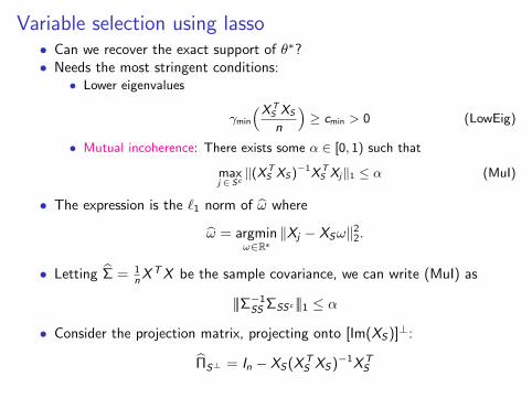
Variable selection using lasso• Can we recover the exact support of θ∗?• Needs the most stringent conditions:

• Lower eigenvalues

γmin

(XTS XS

n

)≥ cmin > 0 (LowEig)

• Mutual incoherence: There exists some α ∈ [0, 1) such that

maxj ∈ Sc

‖(XTS XS)−1XT

S Xj‖1 ≤ α (MuI)

• The expression is the `1 norm of ω where

ω = argminω∈Rs

‖Xj − XSω‖22.

• Letting Σ = 1nX

TX be the sample covariance, we can write (MuI) as

|||Σ−1SS ΣSSc |||1 ≤ α

• Consider the projection matrix, projecting onto [Im(XS)]⊥:

ΠS⊥ = In − XS(XTS XS)−1XT

S

47 / 57

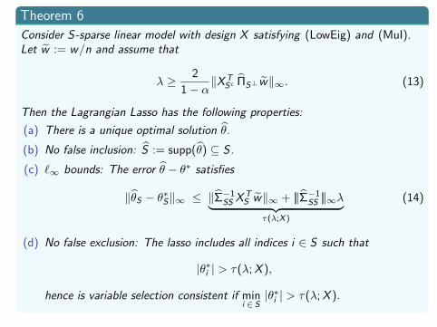
Theorem 6

Consider S-sparse linear model with design X satisfying (LowEig) and (MuI).Let w := w/n and assume that

λ ≥ 2

1− α‖XTSc ΠS⊥w‖∞. (13)

Then the Lagrangian Lasso has the following properties:

(a) There is a unique optimal solution θ.

(b) No false inclusion: S := supp(θ) ⊆ S .

(c) `∞ bounds: The error θ − θ∗ satisfies

‖θS − θ∗S‖∞ ≤ ‖Σ−1SS X

TS w‖∞ + |||Σ−1

SS |||∞λ︸ ︷︷ ︸τ(λ;X )

(14)

(d) No false exclusion: The lasso includes all indices i ∈ S such that

|θ∗i | > τ(λ;X ),

hence is variable selection consistent if mini ∈ S|θ∗i | > τ(λ;X ).

48 / 57

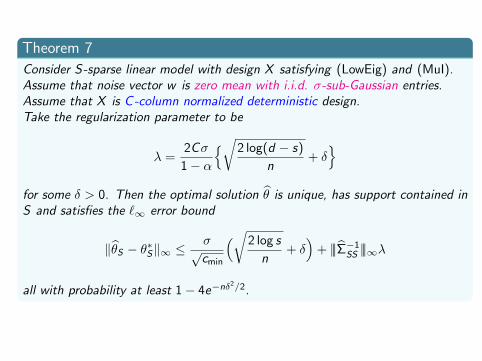
Theorem 7

Consider S-sparse linear model with design X satisfying (LowEig) and (MuI).Assume that noise vector w is zero mean with i.i.d. σ-sub-Gaussian entries.Assume that X is C -column normalized deterministic design.Take the regularization parameter to be

λ =2Cσ

1− α{√2 log(d − s)

n+ δ}

for some δ > 0. Then the optimal solution θ is unique, has support contained inS and satisfies the `∞ error bound

‖θS − θ∗S‖∞ ≤σ√cmin

(√2 log s

n+ δ)

+ |||Σ−1SS |||∞λ

all with probability at least 1− 4e−nδ2/2.

49 / 57

• Need to verify (14): Enough to control

Zj := XTj ΠS⊥w , for j ∈ Sc

• We have ‖ΠS⊥Xj‖2 ≤ ‖Xj‖2 ≤ C√n. (Projections are nonexpansive.)

• Hence, Zj is a sub-Gaussian with squared-parameter ≤ C 2σ2/n. (Exercise.)

• It follows that

P[

maxj∈Sc|Zj | ≥ t

]≤ 2(d − s)e−n t2/(2C 2σ2)

• Choice of λ satisfies (14) with high probability.

• Define ZS = Σ−1S XT

S w . Each Zi = eTi Σ−1S XT

S w is sub-Gaussian withparameter at most

σ2

n|||Σ−1

SS |||op ≤σ2

cminn

• It follows that

P[

maxi=1,...,s

|Zi |︸ ︷︷ ︸‖ZS‖∞

>σ√cmin

(√2 log s

n+ δ)]≤ 2e−nδ

2/2

50 / 57

Exercise

• Assume that w ∈ Rd has independent sub-Gaussian entries,

• with sub-Gaussian squared-parameters ≤ σ2.

• Let x ∈ Rd be a deterministic vector.

• Then, xTw is sub-Gaussian with squared-parameter ≤ σ2‖x‖22.

51 / 57

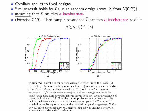
• Corollary applies to fixed designs.• Similar result holds for Gaussian random design (rows iid from N(0,Σ)),• assuming that Σ satisfies α-incoherence.

• (Exercise 7.19): Then sample covariance Σ satisfies α-incoherence holds if

n & s log(d − s)

52 / 57

Detour: subgradients

• Consider a convex function f : Rd → R.

• z ∈ Rd is a sub-gradient of f at θ, denoted z ∈ ∂f (θ) if

f (θ + ∆) ≥ f (θ) + 〈z ,∆〉, ∀∆ ∈ Rd .

• For a convex function θ minimizes f is equivalent to 0 ∈ ∂f (θ).

• For `1 norm, i.e. f (θ) = ‖θ‖1,

z ∈ ∂‖θ‖1 ⇐⇒ zj = sign(θj)

where sign(·) is the generalized sign, i.e. sign(0) = [−1, 1].

• For Lasso, (θ, z) is primal-dual optimal if θ is a minimizer and z ∈ ∂‖θ‖1.

• Equivalently, primal-dual optimality conditions can be written as

1

nXT (X θ − y) + λz = 0, (15)

z ∈ ∂‖θ‖1 (16)

where (15) is the zero subgradient condition.

53 / 57

Proof of Theorem• Primal-dual witness (PDW) construction:

1. Set θSc = 0.

2. Determine (θS , zS) ∈ Rs × Rs by solving oracle subproblem

θS ∈ argminθS∈Rs

1

2n‖y − XSθS‖2

2 + λ‖θS‖1

and choosing zS ∈ ∂‖θS‖1 s.t. ∇f (θS)θS=θS+ λzS = 0.

3. Solve for zSc ∈ Rd−s via zero subgradient equaltion and check for strict dualfeasibility ‖zSc‖∞ < 1.

Lemma 1

Under condition (LowEig) the success of the PDW construction implies that

(θS , 0) is the unique optimal solution of the Lasso.

• Proof: Only need to show uniqueness, which follows from this: Under strongduality, the set of saddle-points of the Lagrangian form a Cartesian product.I.e., we can mix and match primal and dual parts of two primal-dual pair toalso get primal-dual pairs.

54 / 57

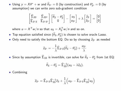
• Using y = Xθ∗ + w and θSc = 0 (by construction) and θ∗Sc = 0 (byassumption) we can write zero sub-gradient condition[

ΣSS ΣSSc

ΣScS ΣScSc

] [θS − θ∗S

0

]−[uSuSc

]+ λ

[zSzSc

]=

[00

]where u = XTw/n so that uS = XT

S w/n and so on.

• Top equation satisfied since (θS , θ∗S) is chosen to solve oracle Lasso.

• Only need to satisfy the bottom EQ. Do so by choosing zSc as needed

zSc = − 1

λΣScS(θS − θ∗S) +

uSc

λ

• Since by assumption ΣSS is invertible, can solve for θS − θ∗S from 1st EQ:

θS − θ∗S = Σ−1SS (uS − λzS).

• Combining

zSc = ΣScS Σ−1SS zS +

1

λ

(uSc − ΣScS Σ−1

SS uS)

55 / 57

• We had

zSc = ΣScS Σ−1SS zS +

1

λ

(uSc − ΣScS Σ−1

SS uS)

• Note that (w = w/n)

uSc − ΣScS Σ−1SS uS = XT

Sc w − ΣScS Σ−1SS X

TS w

= XTSc [I − XS(XT

S XS)−1XTS ]w

= XTSc ΠS⊥w

• Thus, we have

zSc = ΣScS Σ−1SS zS︸ ︷︷ ︸

µ

+XTSc ΠS⊥

( wnλ

)︸ ︷︷ ︸

v

• By (MuI) we have ‖µ‖∞ ≤ α. and by our choice of λ, ‖v‖∞ < 1− α.

• This verifies strict dual feasibility ‖zSc‖∞ < 1, hence the constructed pair isprimal-dual feasible and the primal solution is unique.

56 / 57

• It remains to show the `∞ bound which follows from a applying triangleinequality to

θS − θ∗S = Σ−1SS (uS − λzS).

• leading to

‖θS − θ∗S‖∞ ≤ ‖Σ−1SS uS‖∞ + λ‖Σ−1

SS ‖∞

using sub-multiplicative property of operator norms and ‖z‖∞ ≤ 1.

57 / 57