
PhD Thesis C.R. Huddlestone-Holmes
63
PhD Thesis C.R. Huddlestone-Holmes 92 Chapter 4. Foliation Intersection Axes in porphyroblasts: Understanding your FIA
Transcript of PhD Thesis C.R. Huddlestone-Holmes
PhD Thesis C.R. Huddlestone-Holmes
92
Chapter 4. Foliation Intersection Axes in porphyroblasts: Understanding your FIA
PhD Thesis C.R. Huddlestone-Holmes
93
Abstract A technique that allows the confidence intervals to be assigned to the orientations of
foliation intersection/inflection axes in porphyroblasts (FIA) measured by the asymmetry
method is presented. Parameters, μ (FIA orientation) and β (shape parameter) for a cyclic
logistic regression are calculated using maximum likelihood estimation (MLE). The
bootstrapping of MLE of parameters provides confidence intervals and allow the model fit to be
assessed, and this is demonstrated using several examples.
Analysis of the sensitivity of the bootstrapped MLE approach to the number of
observations per thin section orientation shows that a minimum of 10 are required to produce
accurate results. Detailed studies, which compare the orientation of FIA quantitatively, should
use this technique so that the inferences can be made with confidence. For regional studies, if
the number of samples is sufficient, the distribution of FIA sets (a temporally related grouping
of FIA) can be determined without using the bootstrapped MLE approach as the precision of
individual measurements is less important. This is because the large sample size reduces the
effect of measurement errors. Relative timing criteria and FIA orientations are the best criteria
for grouping data into sets. Using microstructural textures as a criterion is totally unreliable
because deformation partitioning can result in highly variable distributions of strain from grain
to orogen scale.
The distribution of FIAs is similar at both intra-sample and inter-sample scales and is
unimodal, symmetrical and have a peak at their mean with probabilities decaying monotonically
to either side of it, similar to a normal distribution. The maximum range of FIA orientations in a
single set will generally be in the order of 40° to 80°. Consistently grouped FIA distributions
suggest that any rotation of porphyroblasts relative to a fixed geographic reference frame is
unlikely. The distribution of FIAs actually represents the distribution of the foliations that form
them.
1 Introduction FIA (foliation intersection/inflection axes in porphyroblasts) are the axes of curvature
(or intersection) of foliations preserved as inclusion trails in porphyroblasts; they are interpreted
as being equivalent to the intersection lineation between the foliations produced by two
deformation events. This paper examines the significance of FIA data and how it can be applied
to solving geological problems.
FIAs provide a potentially powerful tool for investigating the deformation history of
orogenic belts. Such studies are difficult because the effects of the youngest deformation events
obliterate or reorient structures formed earlier during orogenesis. A window into these older
events is provided by inclusion trails in porphyroblastic minerals. These trails preserve the
PhD Thesis C.R. Huddlestone-Holmes
94
fabrics that were in the rock at their time of formation. Hayward (1990) and Bell et al. (1995)
introduced a method for measuring FIA as a means of quantifying these microstructures.
The quantitative application of FIAs requires consideration of their statistical
significance to ensure that the data are properly understood and that they are not being over
interpreted. Johnson (1999b) suggested that several aspects regarding the measurement and
significance of individual FIA needed clarification. Once individual FIA measurements have
been obtained, their correlation and grouping in a geological region needs to be determined; this
has typically been done by examining the relative timing and orientation of FIAs (e.g. Bell et al.
1998, Yeh & Bell 2004). Stallard et al. (2003) raised concerns about this approach and about the
significance that could be given to a FIA orientation.
This chapter reviews the current literature, defines FIAs, examines the sources of
variation in their orientations on the hand sample and regional scale, describes how to measure
FIAs, and outlines the statistical methods that have been applied to FIA analysis to date. A
technique for quantifying the error in FIA measurements is introduced, and the reliability of
individual FIA measurements is examined. The significance of FIA data at the regional scale is
also considered. Several case studies of the application of FIA data are presented.
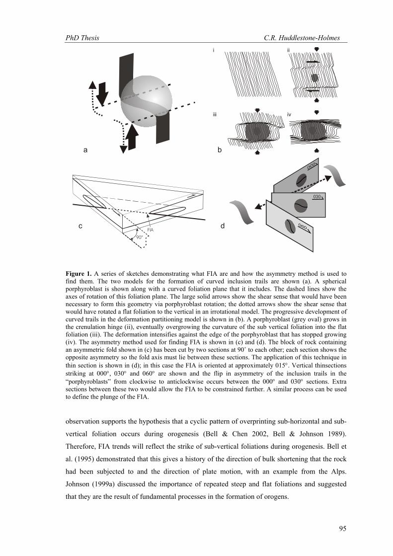
1.1 What is a FIA? The generic description of FIAs states that they are the axis of curvature of curved
inclusion trails within porphyroblasts. While the method for determining the orientation of a
FIA is independent of the processes that formed the curved inclusion trails, their interpretation
is not. According to Hayward (1990) and Bell et al. (1995), a foliation inflection or intersection
axis in a porphyroblast (FIA) is the intersection of successive foliations, or the curvature of one
into the next, which has been overgrown by a porphyroblast (Fig. 1). FIA can be equated with
the intersection lineation between these two foliations or the fold axis of the second event.
Alternatively, they represent the axis of rotation of the porphyroblast while it was growing (e.g.
Rosenfeld 1970). However, there is a growing weight of evidence that firmly suggests
porphyroblast generally do not rotate relative to a fixed geographic reference frame during
ductile deformation (e.g. Aerden 2004, Aerden 1995, Bell & Chen 2002, Bell & Hickey 1999,
Evins 2005, Fyson 1980, Hayward 1992, Johnson 1990, Jung et al. 1999, Steinhardt 1989). This
is an important observation because it means that FIAs preserve the orientations of a range of
fabrics through subsequent deformation events, even though they may be obliterated in the
matrix.
The majority of published FIA data involves trends only. Where plunges have been
measured they are generally sub-horizontal (e.g. Chapter 2`; Bell et al. 1998, Bell & Wang
1999, Hayward 1990, Stallard et al. 2003, Timms 2003). Hayward (1990) argued that this
PhD Thesis C.R. Huddlestone-Holmes
95
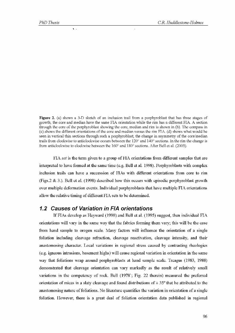
Figure 1. A series of sketches demonstrating what FIA are and how the asymmetry method is used to find them. The two models for the formation of curved inclusion trails are shown (a). A spherical porphyroblast is shown along with a curved foliation plane that it includes. The dashed lines show the axes of rotation of this foliation plane. The large solid arrows show the shear sense that would have been necessary to form this geometry via porphyroblast rotation; the dotted arrows show the shear sense that would have rotated a flat foliation to the vertical in an irrotational model. The progressive development of curved trails in the deformation partitioning model is shown in (b). A porphyroblast (grey oval) grows in the crenulation hinge (ii), eventually overgrowing the curvature of the sub vertical foliation into the flat foliation (iii). The deformation intensifies against the edge of the porphyroblast that has stopped growing (iv). The asymmetry method used for finding FIA is shown in (c) and (d). The block of rock containing an asymmetric fold shown in (c) has been cut by two sections at 90˚ to each other; each section shows the opposite asymmetry so the fold axis must lie between these sections. The application of this technique in thin section is shown in (d); in this case the FIA is oriented at approximately 015°. Vertical thinsections striking at 000°, 030° and 060° are shown and the flip in asymmetry of the inclusion trails in the “porphyroblasts” from clockwise to anticlockwise occurs between the 000° and 030° sections. Extra sections between these two would allow the FIA to be constrained further. A similar process can be used to define the plunge of the FIA.
observation supports the hypothesis that a cyclic pattern of overprinting sub-horizontal and sub-
vertical foliation occurs during orogenesis (Bell & Chen 2002, Bell & Johnson 1989).
Therefore, FIA trends will reflect the strike of sub-vertical foliations during orogenesis. Bell et
al. (1995) demonstrated that this gives a history of the direction of bulk shortening that the rock
had been subjected to and the direction of plate motion, with an example from the Alps.
Johnson (1999a) discussed the importance of repeated steep and flat foliations and suggested
that they are the result of fundamental processes in the formation of orogens.
i ii
iii iv
ba
FIAc
90°
030
d
jc151654
Text Box
THIS IMAGE HAS BEEN REMOVED DUE TO COPYRIGHT RESTRICTIONS
PhD Thesis C.R. Huddlestone-Holmes
97
studies. In general, where the effects of later deformations can be ruled out, the data have
clustered distributions,.
FIA may be curved or offset because the foliations that form them wrap around pre-
existing porphyroblasts. Hayward (1990`; fig 6.) suggested that this may result in as much as
45º of angular deviation of the foliation. This variation would happen on the scale of a
porphyroblast with the orientation of the foliation affected by the different crystal faces. All of
these sources of variation in FIA orientations are most likely normally distributed. An exception
is where a crenulation cleavage preserves a relict foliation in its hinges. In this case the FIA may
have a bimodal distribution or be skewed.
If FIAs form by rotation of porphyroblasts as they grow then the distribution of FIAs
formed in a single foliation-forming event would also show a normal distribution, assuming the
porphyroblasts were not rotated by subsequent events. If the porphyroblasts are affected by
subsequent deformation events it is highly probable that the amount an individual porphyroblast
rotates will vary because of the heterogeneity of strain and the interference of other grains
(Beirmeier & Stuwe 2003). This variation in rotation would lead to a girdle like distribution
after a single overprinting event and subsequent events would lead to a random distribution
(Ham & Bell 2004). The growing body of FIA data with non-random data distributions (e.g.
Bell et al. 2004, Bell et al. 1998, Stallard et al. 2003, Yeh & Bell 2004) strongly suggests that
rotation is an unlikely mechanism for their formation.
If FIAs do form as a result of overprinting foliations then deformation partitioning may
complicate matters further. Bell and Hayward (1991) describe how deformation partitioning can
be used to explain how simple and complex inclusion trails can coexist in the same outcrop.
They argue that porphyroblast growth only occurs in zones actively undergoing deformation;
that simple inclusion trails form in zones microfolded by one episode of foliation development
and porphyroblast growth and complex trails form where these episodes are repeated. It is
therefore conceivable that a rock that has undergone multiple foliation forming events will have
FIAs equivalent to .....,,,,, 34
24
14
23
13
12 LLLLLL and so on (terminology from Bell & Duncan
1978). Accepting that a cyclic pattern of overprinting sub-horizontal and sub-vertical foliations
can develop, this deformation partitioning argument should be able to generate FIAs with a sub-
vertical plunge. FIA at this orientation would only occur if two vertical foliations form it that
are at a high angle to each other. This case would be readily identified because vertical thin
sections would contain coaxial geometries regardless of their orientation while horizontal
sections would contain asymmetrical geometries. When the two overprinting foliations are at a
low angle to each other, the second is likely to reactivate the first and porphyroblast growth is
unlikely (Bell 1986, Bell et al. 2004).
PhD Thesis C.R. Huddlestone-Holmes
98
1.3 Statistics of FIAs – Exisiting Work Despite the growing body of literature using FIA data, there is little written on the
statistical significance of FIA. Bell and Hickey (1997) briefly discussed the accuracy of FIA
determinations due to measurement errors. They determined that the total accumulated
analytical error in collecting an oriented sample, reorienting it and preparing the thin sections
was ± 8º. This error is expected to have a normal distribution. Bell et al. (1998) discussed some
of the aspects of analysis of regional FIA datasets. They employ Watson’s U2 test modified for
grouped data to confirm whether the FIA data come from a random population and a chi-
squared test to confirming whether FIA sets differ significantly from each other. Yeh (2003) and
Yeh and Bell (2004) applied these tests and also implemented a moving average method to
discern peaks in FIA data from a region. None of these tests address the distribution of FIAs
within a sample, or on a regional scale, except to show that they do not represent a random
distribution and that FIA sets can be differentiated from each other. Yeh and Bell (2004) also
commented that the variation of FIA orientations in a FIA set ranges from 30º to 50º based on a
review of published data. They argue that this distribution is a result of the anastomosing nature
of foliations.
The asymmetry method for measuring FIAs determines them for a sample rather than
for individual porphyroblasts. Consequently, meaningful estimates of the distribution of FIAs in
a sample have not been possible using that approach. Typically FIA measurements have been
reported as the mid-point of the range over which the dominant asymmetry flips with no
indication of the spread within a sample. Stallard et al. (2003) demonstrated a technique for
quantifying the reliability of FIA measurements using data for samples collected from Georgia,
USA. They used a method developed by Upton et al. (2003) for the analysis of cyclic logistic
data using a maximum likelihood technique to fit a regression model to the asymmetry data.
They argued that the range over which FIAs occur in a single sample is in the order of 50º.
Chapter 3 demonstrates several flaws in the assumptions in Upton et al.’s (2003) approach and
presents a more robust technique using bootstrapping. This technique is summarised in the
methods section. Upton et al. (2003) express some concern on the reliability of the technique for
samples in which only a small number of observations have been made and this issue is
examined in more detail below.
2 Methods
2.1 How are FIAs Determined? The asymmetry method most commonly used for determining FIA orientations was first
described Hayward (1990) and then expanded to include plunges by Bell et al. (1995). The
method relies on the fact that a simple asymmetrically folded surface with a sub-horizontal axis
PhD Thesis C.R. Huddlestone-Holmes
99
will appear to have opposite asymmetries when cut by two vertical planes that strike either side
of the fold axis (Fig. 1c`; Bell et al. 1998). The fold asymmetry appears anticlockwise in one
(“Z”, left side of Fig. 1c) and clockwise in the other (“S”, right side of Fig. 1c). Note that both
these planes are viewed in the same direction – for example clockwise about a vertical axis.
Curved inclusion trails preserved in porphyroblasts are analogous to such a fold. Figure 1d
shows how this concept is applied in thin-sections. The trend of the FIA is constrained to lie
between two vertical thin sections with a close angular spacing which have the opposite
observed dominant asymmetries. Sections are typically cut at a 10˚ angular spacing and the FIA
trend is recorded as being midway point of this interval. In some cases a thin section may have
both asymmetries in equal proportions, with sections either side having opposite asymmetries
dominating. When this occurs, the FIA is interpreted to be parallel to the thin section. Once the
trend of a FIA in a sample has been determined, the plunge can be found using a similar
approach. A series of sections perpendicular to the vertical plane containing the FIA trend with
different dips are cut; the FIA plunge is determined as being between the two sections across
which the inclusion trail asymmetry changes.
Powell and Treagus (1967) were the first to publish a method of determining what are
now called FIAs in garnet using thick sections and a universal stage. Busa and Graham (1992)
used a similar technique looking at staurolite grains. These techniques are inaccurate as they
only measure a short segment of the axis and make assumptions about the relationship between
the elongation of included grains and the orientation of the FIA. Rosenfeld (1970) described
several techniques for finding FIAs. These methods were in part based on the assumption that
curved trails are the result of porphyroblast rotation. His techniques included one for finding the
FIA in a single large porphyroblast (tens of millimetres in diameter) that is not practical for the
majority of rocks that have smaller porphyroblast sizes, or those with multiple FIAs. For these
rocks he used a method based on the same asymmetry principle as used later by Hayward
(1990). However, he used the main schistosity in the rock as the reference plane (i.e. all sections
cut perpendicular to the main schistosity in the rock) instead of the horizontal. This was based
on the flawed assumption that the matrix foliation was the one that formed the curved inclusion
trails. If the actual FIA orientation lies at a high angle to this schistosity it would be difficult to
constrain it with this approach. There is no way of determining whether this schistosity was the
dominant one at the time of porphyroblast growth. The asymmetry method allows the trend of a
FIA to be determined in all cases except those rare cases with a vertical or near-vertical plunge.
Determining a FIA orientation is complicated when more than one FIA are preserved in
a sample. Figure 2a shows an inclusion trail that has two distinct FIAs lying at an angle to each
other. Depending on the orientation of the thin section, either a staircase or spiral geometry will
be observed (Fig. 2d). Such samples provide valuable relative timing criteria for FIAs as those
in the core of the garnets must form before those in their outer parts. See Fig.3 for an example.
PhD Thesis C.R. Huddlestone-Holmes
100
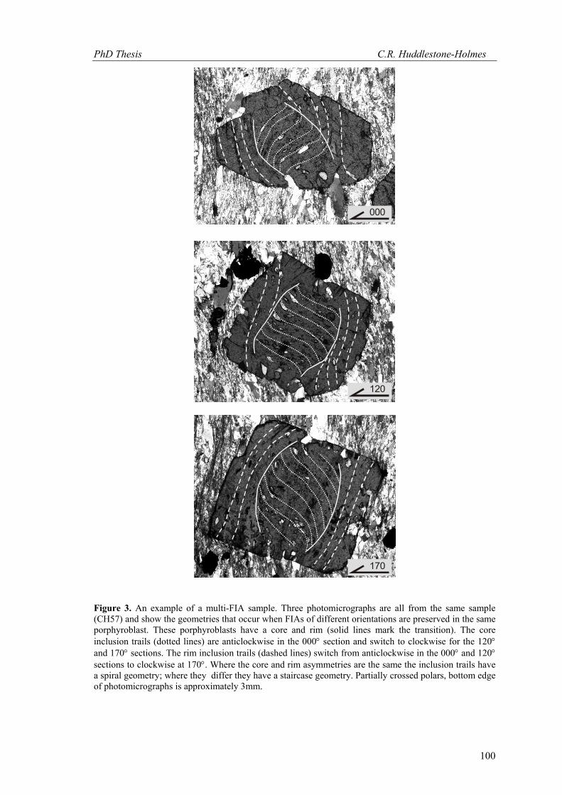
Figure 3. An example of a multi-FIA sample. Three photomicrographs are all from the same sample (CH57) and show the geometries that occur when FIAs of different orientations are preserved in the same porphyroblast. These porphyroblasts have a core and rim (solid lines mark the transition). The core inclusion trails (dotted lines) are anticlockwise in the 000° section and switch to clockwise for the 120° and 170° sections. The rim inclusion trails (dashed lines) switch from anticlockwise in the 000° and 120° sections to clockwise at 170°. Where the core and rim asymmetries are the same the inclusion trails have a spiral geometry; where they differ they have a staircase geometry. Partially crossed polars, bottom edge of photomicrographs is approximately 3mm.
000
120
170
PhD Thesis C.R. Huddlestone-Holmes
101
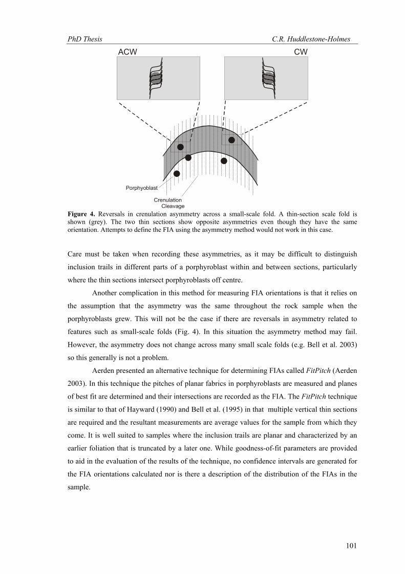
Figure 4. Reversals in crenulation asymmetry across a small-scale fold. A thin-section scale fold is shown (grey). The two thin sections show opposite asymmetries even though they have the same orientation. Attempts to define the FIA using the asymmetry method would not work in this case.
Care must be taken when recording these asymmetries, as it may be difficult to distinguish
inclusion trails in different parts of a porphyroblast within and between sections, particularly
where the thin sections intersect porphyroblasts off centre.
Another complication in this method for measuring FIA orientations is that it relies on
the assumption that the asymmetry was the same throughout the rock sample when the
porphyroblasts grew. This will not be the case if there are reversals in asymmetry related to
features such as small-scale folds (Fig. 4). In this situation the asymmetry method may fail.
However, the asymmetry does not change across many small scale folds (e.g. Bell et al. 2003)
so this generally is not a problem.
Aerden presented an alternative technique for determining FIAs called FitPitch (Aerden
2003). In this technique the pitches of planar fabrics in porphyroblasts are measured and planes
of best fit are determined and their intersections are recorded as the FIA. The FitPitch technique
is similar to that of Hayward (1990) and Bell et al. (1995) in that multiple vertical thin sections
are required and the resultant measurements are average values for the sample from which they
come. It is well suited to samples where the inclusion trails are planar and characterized by an
earlier foliation that is truncated by a later one. While goodness-of-fit parameters are provided
to aid in the evaluation of the results of the technique, no confidence intervals are generated for
the FIA orientations calculated nor is there a description of the distribution of the FIAs in the
sample.
ACW CW
Porphyoblast
Crenulation Cleavage
PhD Thesis C.R. Huddlestone-Holmes
102
2.2 Maximum Likelihood Estimation of FIA Parameters In order to provide a test of the statistical significance of a FIA measurement
determined using the asymmetry method, a parametric model is fitted to the data. The
parametric model used is the logistic model that was suggested by Upton et al. (2003). It relates
the probability p of observing a particular asymmetry (clockwise or anticlockwise) in a thin
section with orientation θ to the trend of the FIA (μ) and a shape parameter (β). The probability
density function for the logistic model is
( ) )sin(
)sin(
1,, μθβ
μθβ
μβθ −
−
+=
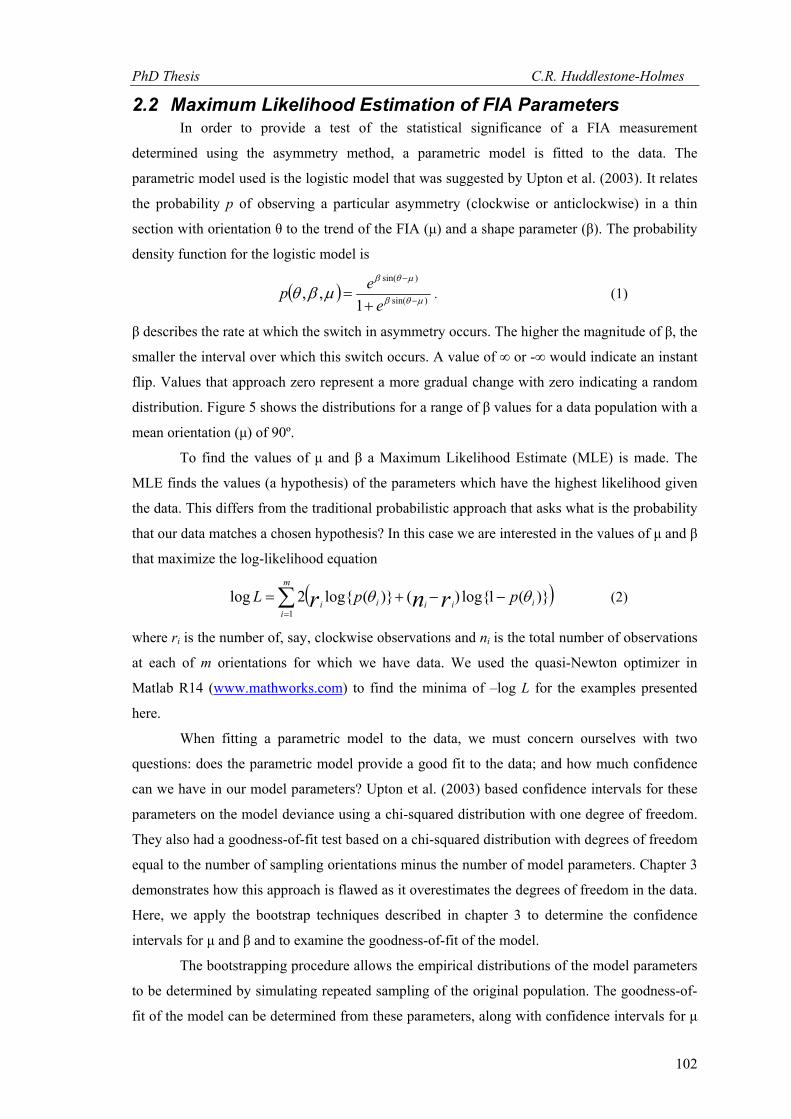
eep . (1)
β describes the rate at which the switch in asymmetry occurs. The higher the magnitude of β, the
smaller the interval over which this switch occurs. A value of ∞ or -∞ would indicate an instant
flip. Values that approach zero represent a more gradual change with zero indicating a random
distribution. Figure 5 shows the distributions for a range of β values for a data population with a
mean orientation (μ) of 90º.
To find the values of μ and β a Maximum Likelihood Estimate (MLE) is made. The
MLE finds the values (a hypothesis) of the parameters which have the highest likelihood given
the data. This differs from the traditional probabilistic approach that asks what is the probability
that our data matches a chosen hypothesis? In this case we are interested in the values of μ and β
that maximize the log-likelihood equation
( )∑=
−−+=m
iiiiii ppL rnr
1)}(1log{)()}(log{2log θθ
(2)
where ri is the number of, say, clockwise observations and ni is the total number of observations
at each of m orientations for which we have data. We used the quasi-Newton optimizer in
Matlab R14 (www.mathworks.com) to find the minima of –log L for the examples presented
here.
When fitting a parametric model to the data, we must concern ourselves with two
questions: does the parametric model provide a good fit to the data; and how much confidence
can we have in our model parameters? Upton et al. (2003) based confidence intervals for these
parameters on the model deviance using a chi-squared distribution with one degree of freedom.
They also had a goodness-of-fit test based on a chi-squared distribution with degrees of freedom
equal to the number of sampling orientations minus the number of model parameters. Chapter 3
demonstrates how this approach is flawed as it overestimates the degrees of freedom in the data.
Here, we apply the bootstrap techniques described in chapter 3 to determine the confidence
intervals for μ and β and to examine the goodness-of-fit of the model.
The bootstrapping procedure allows the empirical distributions of the model parameters
to be determined by simulating repeated sampling of the original population. The goodness-of-
fit of the model can be determined from these parameters, along with confidence intervals for μ
PhD Thesis C.R. Huddlestone-Holmes
103
Section Orientation
0 10 20 30 40 50 60 70 80 90 100
110
120
130
140
150
160
170
180
prob
abili
ty
0.0
0.2
0.4
0.6
0.8
1.0
0=β
1=β
2=β
3=β
5−=β
5=β
10=β
8=β
5.0=β
50=β20=β
Figure 5. Graph showing the probability of a success at a given section orientation for different values of β according to the cyclic logistic model; a success is arbitrarily defined as observing a particular asymmetry (e.g. clockwise). Higher values of β show a more rapid change in asymmetry. μ = 90º in all cases. The dashed line shows that the sign of β determines whether the switch is from “successes” to “failures” or vice versa.
and β. Goodness-of-fit is determined informally by inspecting the distributions of μ and β,
which should be normal or log normal, plus the deviance which should have some form of chi-
squared distribution whose degrees of freedom will be less than or equal to m-2. Confidence
intervals for the model parameters μ and β are determined from the bootstrapped data by the
percentile method adjusted for bias and acceleration (BCa) as discussed in Chapter 3. Two
bootstrapping methods can be applied. One resamples within section orientations (method A)
and the other across section orientations (method B; see chapter 3). Which of these methods
produces a better model fit will depend on the nature of the sample population. Method B is
preferred, except where the total number of observations is small.
PhD Thesis C.R. Huddlestone-Holmes
104
2.2.1 Implementation of MLE The MLE technique described above and in chapter 3 attempts to find the parameters μ
and β of a cyclic logistic model that fits the data. Before we can interpret the geological
meaning of these values, we have to be sure that the cyclic logistic model is a good fit. If it is
not, these parameters may be meaningless. Graphical procedures are used to assess the
goodness-of-fit of the model to the data. To demonstrate the MLE technique, asymmetry data
was generated for sample V209, based on the measurements obtained using HRXCT in chapter
2 (Appendix 1.1). This was done by determining what asymmetries would be observed if all 58
garnets measured were intersected by thin sections cut at 10º increments from 0º to 170º. The
resulting asymmetry data is a perfect representation of the sampled data, free from observation
errors or sampling bias. There is a large number of observations (N = 58) and the sample is
unimodal and symmetrical about its mean.
Figure 6 shows the results of the bootstrap MLE analysis of this data. The distributions
of μ and β are normal and lognormal respectively indicating that they are well represented by
the logistic model. The deviance plot shows a chi-squared distribution with approximately five
degrees of freedom. While this distribution, combined with those for μ and β, may be enough to
satisfy us that the model is a good fit for the data, we can gain further confidence by examining
a boxplot of the deviance (Fig. 6e). The boxplot shows that for a number of section orientations
(60º through 160º) there is very little variation in probability of a given observation. This lack of
variance means that only seven orientations contribute to the freedom of the data to vary. The
number of degrees of freedom for the deviance should be five because the values of two
parameters (μ and β) are fixed. A chi-squared distribution with five degrees of freedom matches
the distribution observed, so we can be very confident that the data is well represented by the
logistic model with the values for μ and β calculated.
Given that the proposed model has a good fit for the data, we can now determine the
confidence intervals for the parameters μ and β. Because the data is so well behaved the
percentile method can be used. For a 95% confidence interval the parameter values at 2.5% and
97.5% of the bootstrap distributions are taken. Unlike a normal distribution for linear data these
values cannot be directly related to the shape of the distribution; they simply represent the
confidence that can be placed in the mean values calculated for μ and β. The parameter β
describes the spread of the data and is analogous to the concentration parameter kappa of a von
Mises distribution.
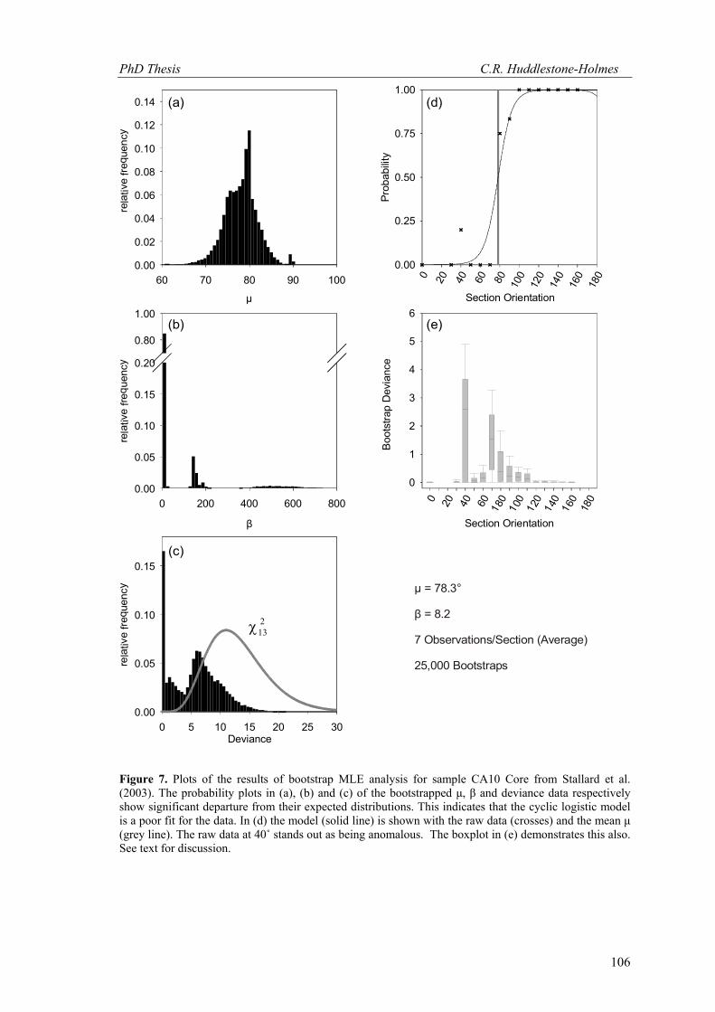
For comparison, Figure 7 shows the results of using the bootstrap MLE approach for the
sample CA10 Core from Stallard et al. (2003, see also Appendix 1.2). In this case, the cyclic
logistic model is a poor fit for the data. This is demonstrated by the departure from normal of
the μ and β distributions and the multiple peaks in the deviance distribution. The hypothesis that
the cyclic logistic model can be used to describe this data must be rejected and confidence

PhD Thesis C.R. Huddlestone-Holmes
105
Figure 6. Plots of the results of bootstrap MLE analysis for the HRXCT data from sample V209. (a), (b)
and (c) are probability plots of the bootstrapped μ, β and deviance data respectively. The distributions of
μ and β are normal and log-normal respectively. The deviance has a distribution that is approximated by a
chi-squared distribution with 5 degrees of freedom. These distributions indicate that the cyclic logistic
model is a good fit for the data. In (d) the model (solid line) is shown with the raw data (crosses) and the
mean μ (grey line). The boxplot in (e) demonstrates that only some of the sections contribute to the
variability of the data. 95% confidence intervals for μ and β in brackets.
0 5 10 15 20 25 300.00
0.05
0.10
6 8 10 12 140.00
0.02
0.04
0.06
0.08
0.10
25χ
216χ
Section Orientation
- - - 1
Prob
abili
ty
60 40 20 0 20 40 60 80 00
0.00
0.25
0.50
0.75
1.00(d)
(c)
(b)
rela
tive
frequ
ency
16 18 20 22 240.00
0.02
0.04
0.06
0.08(a)
μ
β
Deviance
μ = 20.4° (18.3°, 20.4°)
β = 9.4 (7.7, 11.0)
58 Observations/Section
25,000 Bootstraps
rela
tive
frequ
ency
Section Orientation
-60
-40
-20 0 20 40 60 80 100
0
1
2
3
4(e)
Boo
tstra
p D
evia
nce
r ela
tive
frequ
ency
PhD Thesis C.R. Huddlestone-Holmes
106
Figure 7. Plots of the results of bootstrap MLE analysis for sample CA10 Core from Stallard et al. (2003). The probability plots in (a), (b) and (c) of the bootstrapped μ, β and deviance data respectively show significant departure from their expected distributions. This indicates that the cyclic logistic model is a poor fit for the data. In (d) the model (solid line) is shown with the raw data (crosses) and the mean μ (grey line). The raw data at 40˚ stands out as being anomalous. The boxplot in (e) demonstrates this also. See text for discussion.
µ60 70 80 90 100
0.00
0.02
0.04
0.06
0.08
0.10
0.12
0.14
Deviance0 5 10 15 20 25 30
rela
t ive
freq u
ency
0.00
0.05
0.10
0.15
β
0 200 400 600 800
rela
t ive
freq u
ency
0.00
0.05
0.10
0.15
0.20
0.80
1.00
rela
t ive
freq u
ency
213χ
Section Orientation
0 20 40 60 80 100
120
140
160
180
Prob
abili
ty
0.00
0.25
0.50
0.75
1.00
Section Orientation
0 20 40 60 801 001 201 401 60 180
0
1
2
3
4
5
6(e)
(d)
(c)
(b)
(a)
1
Boo
tstra
p D
evia
nce
μ = 78.3°
β = 8.2
7 Observations/Section (Average)
25,000 Bootstraps
PhD Thesis C.R. Huddlestone-Holmes
107
intervals for μ and β cannot be determined using the bootstrap technique. There are several
explanations for the poor fit of the model. First is sampling error, whereby asymmetry
observations have been misinterpreted. Examples of this are confusing trails in the median with
those in the core of a garnet, or simply getting the asymmetry wrong. Second, the underlying
FIA population may not have a distribution that can be described using the cyclic logistic
model. This could result from mixed populations being sampled, or the underlying population
has a girdle rather than clustered distribution. Third is that the sample is not representative of
the true population. If the number of observations is small, particular in the region of the FIA,
random chance may result in a biased sample. This may be the case for the CA10 Core data. For
example, in the 40º section there are only five observations. The true probability of a clockwise
observation may be lower than 0.2 but there are insufficient observations to demonstrate this.
The locations of the thin sections may also introduce bias into the sample if the population
distribution varies through the specimen.
Even though our chosen model cannot describe the CA10 core data, it would be
possible to conclude that the true orientation of μ must be between 60º and 90º from studying
the bootstraped μ distribution; therefore, the calculated mean of 78.3 is reasonable. Caution
must be exercised here in case the cause of the poor fit of the model is a result of some
geological process rather than sampling irregularities.
2.2.2 Sensitivity to Sample Size As for all statistical tests, the MLE cyclic logistic regression technique described above
is sensitive to the number of observations that make up the sample. Applying bootstrap methods
addresses this issue by creating many samples of the original data population based on the
original sample; however, bootstrapping cannot improve on a sample that was unrepresentative
of the sampled population in the first place. There will be some minimum amount of data that
will be required to adequately describe the underlying distribution. This issue has been
examined to attempt to provide guidance on the minimum number of observations that should
be obtained to provide a representative sample for measuring FIAs.
A modified bootstrapping technique was used to test the sensitivity of the MLE of the
model parameters to the number of observations. Strictly speaking, the bootstrap method
involves resampling of the original sample, 0θ , with each resample jθ containing the same
number of observations as the original data. In this case, we are interested to see what the effect
of the number of observations has on the values we obtain for μ, β and their confidence
intervals. To do this we take a sub-sample, Niθ , with N observations of the original data and
then perform the bootstrap technique described in chapter 3, substituting Niθ for 0θ ; the
bootstrap is performed B times and for each bootstrapped sample, BjjNi ...1, =θ , we calculate

PhD Thesis C.R. Huddlestone-Holmes
108
4 6 8 10 12 14 16 18 20 25 30 35 40
β
-200
-100
0
100
200
300
400
500
600
N
4 6 8 10 12 14 16 18 20 25 30 35 40
μ
10
15
20
25
30
35
4 6 8 10 12 14 16 18 20 25 30 35 40
Sta
ndar
d D
evia
tion
in β
-100
0
100
200
300
400
N
4 6 8 10 12 14 16 18 20 25 30 35 40
Sta
ndar
d D
evia
tion
in μ
0
1
2
3
4
5
6
7
Figure 8. Plots of sample size sensitivity analysis for the HRXCT data from sample V209. Mean values for μ and β are shown in (a) and (b) and standard deviations in (c) and (d). Error bars show 95% confidence intervals. See text for further discussion.
MLE for jNiβ and j
Niμ . This process is repeated i times for each N allowing the distributions of
jNβ and j
Nμ to be determined. For these tests B = 2000, i = 100 and N varies from 3 to 40.
The results of these tests are plotted in Figure 8 for the data from the HRXCT study of
sample V209. This data was has 58 observations in each section orientation and is well
described by a cyclic logistic regression. The plots of the mean values of μ and β (Fig.8a and b)
display asymptotically decreasing confidence intervals with increasing N as expected. The point
at which the amount of variability decreases to some limit is at around N = 15 in this sample.
The standard deviation plots (Fig.8c and d) show a similar trend; this indicates that the data is
approaching a point that represents the natural variability in the sample. As N increases the
standard deviation for β stabilizes while that for μ continues to decrease.
This technique has been applied to twelve other datasets from eight different samples.
These datasets were selected because the number of observations was high and the bootstrap
MLE analysis showed that the cyclic logistic model fits the data well. The results are shown in
Appendix 2. In general, these data demonstrate that the minimum number of observations
PhD Thesis C.R. Huddlestone-Holmes
109
required to represent the sampled population is between eight and fifteen. They all show the
same pattern of the standard deviation for β stabilizing while that for μ continues to decrease.
The increase in confidence in the mean of μ, by increasing the number of observations much
above ten, is less than a few degrees.
In some cases, N was allowed to exceed the number of observations in the original
sample. This resulted in an over sampling of the data causing spurious results with variability
increasing at higher N (e.g. CH2, CH22, CH49). While these results are included in Appendix 2,
the over sampled parts on the plots were not considered for this interpretation.
3 Examples The bootstrap MLE approach gives a method in which the distribution of FIAs in a
single sample can be measured. It allows confidence intervals to be assigned to these
measurements. None of the published literature containing FIA data include such statistical
analysis, with the exception of Stallard et al. (2003). Some examples of the application of the
technique are explored to investigate the importance of such an analysis where FIA data are
used are given in the following section.
3.1 Stallard et al. Data Stallard et al. (2003) presented the first application of a MLE technique to the analysis
of FIA data collected by the asymmetry method. They examine data collected from 25 samples
from the Canton Schist in the Southern Blue Ridge, Georgia. 61 FIAs were determined with 14
samples containing core, media and rim FIAs that allowed the relative timing to be determined.
The MLE technique used was that detailed by Upton et al. (2003). As discussed above and in
chapter 3 this technique is flawed, particularly in regard to the goodness-of-fit test. Stallard et
al. (2003) state that in all cases the goodness-of-fit was acceptable; however, using the bootstrap
techniques outlined in chapter 3, very few if any of their data can be modelled using the cyclic
logistic model (Fig. 7; Figs. 3 and 4 of Chapter 3). This poor fit appears to be due to the small
sample sizes used in their study in which there are only two or three observations per section
orientation. Stallard et al. (2003) note they have samples with wide 95% confidence limits. This
is most likely the result of sparse sampling where chance results in an apparently anomalous
observation whose influence would be reduced if the number of observations were increased.
As a result the 95% confidence intervals they present are unreliable. However, they observe that
the true intra sample FIA spread is likely to be in the range of 30˚-50˚; this is not unreasonable
compared to the results of the HRXCT study in Chapter 2.
In the second part of their paper, Stallard et al. (2003) investigate approaches to
correlating FIAs between samples. They suggest three possible approaches; using relative
timing and textural criteria; using orientation, relative timing and patterns of changing FIA
jc151654
Text Box
THIS IMAGE HAS BEEN REMOVED DUE TO COPYRIGHT RESTRICTIONS
PhD Thesis C.R. Huddlestone-Holmes
111
Looking at the data of Stallard et al. (2003) in more detail, only 14 of the 25 samples
analysed had sufficient rim growth to be analysed, as the other 11 did not preserve what was
interpreted as being a pervasive deformation event. The distribution of sample localities consists
of a cluster of 19 samples in the immediate vicinity of Canton (Fig. 9), with two samples (CA9
and CA10) well to the south west, three (CA19, CA20 and CA23) over 10km to the north east,
and one sample (CA37) over 20km to the north east. It is interesting to note that none of the
samples located outside the cluster near Canton have data reported for rim FIAs given that the
core-rim transition is used as a temporal marker for all samples (Fig. 9). This demonstrates the
problems of trying to use inclusion trail textures as temporal markers between samples.
Deformation partitioning can result in highly variable distributions of strain from grain to
orogen scale (e.g. Bell et al. 2004) making features such as the intensity of a foliation preserved
in porphyroblasts totally unreliable for such correlations.
A significant consequence of Stallard et al. (2003) using textural criteria for the
interpretation of FIA data was that supposedly temporally related FIAs have a spread of
orientations of greater than 140˚. This then raises the question of what FIAs are. If they do
represent the intersection/inflection axis between foliations then Stallard et al. (2003) are
suggesting that a foliation may vary by up to 140˚ as it forms. They list the possible sources of
variation in foliation orientation as: heterogeneous rheology (i.e., refraction); rotation of the
kinematic reference frame; anastomosing of foliations around inhomogeneities such as granites;
and rotation of porphyroblasts relative to each other. No literature documents the range of
orientations a single foliation can have; however, a 140˚ spread appears as implausible as
suggesting that the cores of all garnets in a field area grew at the same time. A rotation
argument is difficult to reconcile with the clustered nature of the data in Stallard et al. (2003)
and the consistently shallow plunges they have reported. Bell et al. (2004) give an example of
how deformation partitioning provides a mechanism for variation in FIA orientations preserved
in the cores of porphyroblasts and throughout their growth. Another important issue is that a
FIA set represents FIAs with similar orientations and need not represent a single foliation-
forming event. Studies demonstrating that spiral inclusion trails form as the result of
porphyroblasts overgrowing many foliation events with similar strikes are an example of this
(Bell et al. 1992, Johnson 1993). Such sequences of foliations result from the direction of bulk
shortening remaining constant for a period. FIAs that form over such a long period may show
some variation in orientation due to slight variations in the bulk shortening direction that are too
small to distinguish.
Using the orientations of FIAs along with relative timing removes the subjectivity
involved in attempting to correlate textures. Figure 10 shows a reinterpretation of the FIA data
in Stallard et al. (2003) using this method; this is the same approach as their method 3. In this
case four distinct FIA sets have been differentiated based on analysis of the non-parametric
PhD Thesis C.R. Huddlestone-Holmes
113
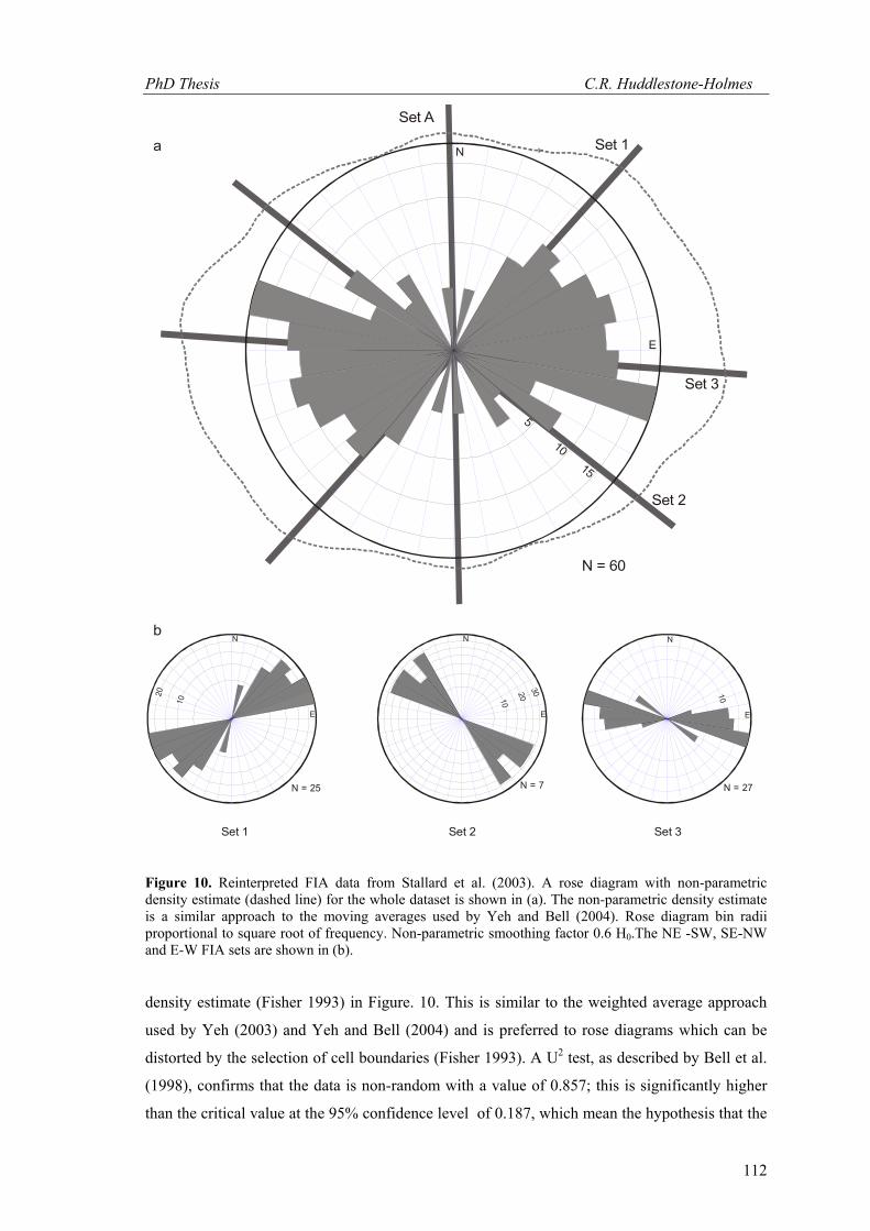
data is from a random distribution can be rejected.. A north-south FIA set is attributed to CA19a
and CA20 and the relative timing of this set cannot be determined as this orientation was only
reported for single FIA samples. Relative timing criteria for the other three sets suggest a
progression from, NE-SW to SE-NW to E-W sets. Each set has a spread of less than 70˚. These
spreads are comparable to those in the other studies cited above. This is despite the fact that the
FIA measurements in Stallard et al. (2003) are based on a small number of observations in each
sample that would be prone to sampling error.
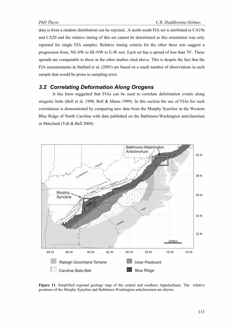
3.2 Correlating Deformation Along Orogens It has been suggested that FIAs can be used to correlate deformation events along
orogenic belts (Bell et al. 1998, Bell & Mares 1999). In this section the use of FIAs for such
correlations is demonstrated by comparing new data from the Murphy Syncline in the Western
Blue Ridge of North Carolina with data published on the Baltimore-Washington anticlinorium
in Maryland (Yeh & Bell 2004).
Figure 11. Simplified regional geology map of the central and southern Appalachians. The relative positions of the Murphy Syncline and Baltimore-Washington anticlinorium are shown.
Coastal
Plain
88 W 86 W 84 W 82 W 80 W 78 W 76 W 74 W
32 N
34 N
36 N
38 N
40 N
Raleigh Goochland Terrane
Carolina Slate Belt
Inner Piedmont
Blue Ridge
MurphySyncline
Baltimore-WashingtonAnticlinorium
Valley and
Ridge
Cumberland
Plateau
200km
PhD Thesis C.R. Huddlestone-Holmes
114
3.2.1 Geological Setting – Murphy Syncline The Murphy Syncline extends from south-west North Carolina into northern Georgia
and nearby Tennessee (Fig. 11). It forms part of the western Blue Ridge of the Appalachian
Orogeny (Hatcher 1987) and is bounded to the east by the Hayesville Fault and to the west by
the Great Smoky and Greenbrier Faults. The rocks in the study area are meta-sediments from
the late Pre-Cambrian to early Cambrian Murphy Belt and Great Smoky Groups (Hatcher 1987,
Mohr 1973, Wiener & Merschat 1992). The Murphy Syncline is isoclinal with a moderately
southeast dipping axial plane. Mohr (1973) suggests that the Murphy Syncline is a D1 structure,
which formed either prior to or during the peak of regional metamorphism. Metamorphic grade
ranges from green schist to amphibolite facies, with the lowest grades in the core of the
syncline. The metamorphic peak in the western Blue Ridge was thought to have been reached
during the Taconic orogeny at approximately 450 Ma, with little if any effect from either the
Acadian or Alleghanian orogenies (e.g. Glover et al. 1983, Hatcher 1987, Rodgers 1987).
However, Unrug and Unrug (1990) and Tull et al. (1993) have argued that the peak of
metamorphism was in a single Acadian event based on fossil assemblages, as do recent electron
probe micro-analyser (EPMA) age dates obtained from monazite (Kohn & Malloy 2004).
Connelly and Dallmeyer (1993) argue for a polymetamorphic history involving both Taconic
and Acadian events.
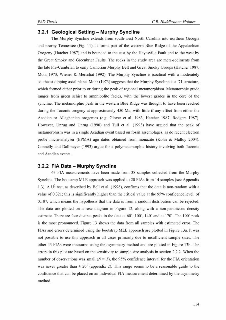
3.2.2 FIA Data – Murphy Syncline 63 FIA measurements have been made from 38 samples collected from the Murphy
Syncline. The bootstrap MLE approach was applied to 20 FIAs from 14 samples (see Appendix
1.3). A U2 test, as described by Bell et al. (1998), confirms that the data is non-random with a
value of 0.321; this is significantly higher than the critical value at the 95% confidence level of
0.187, which means the hypothesis that the data is from a random distribution can be rejected.
The data are plotted on a rose diagram in Figure 12, along with a non-parametric density
estimate. There are four distinct peaks in the data at 60˚, 100˚, 140˚ and at 170˚. The 100˚ peak
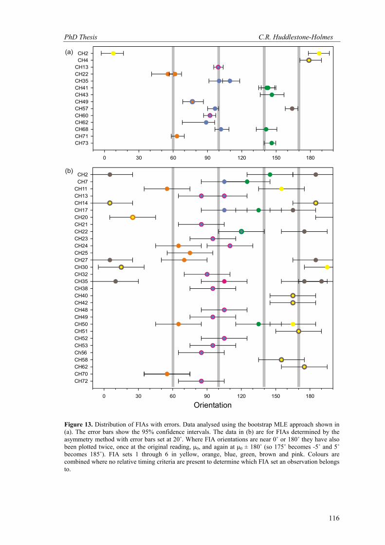
is the most pronounced. Figure 13 shows the data from all samples with estimated error. The
FIAs and errors determined using the bootstrap MLE approach are plotted in Figure 13a. It was
not possible to use this approach in all cases primarily due to insufficient sample sizes. The
other 43 FIAs were measured using the asymmetry method and are plotted in Figure 13b. The
errors in this plot are based on the sensitivity to sample size analysis in section 2.2.2. When the
number of observations was small (N = 3), the 95% confidence interval for the FIA orientation
was never greater than ± 20˚ (appendix 2). This range seems to be a reasonable guide to the
confidence that can be placed on an individual FIA measurement determined by the asymmetry
method.
PhD Thesis C.R. Huddlestone-Holmes
115
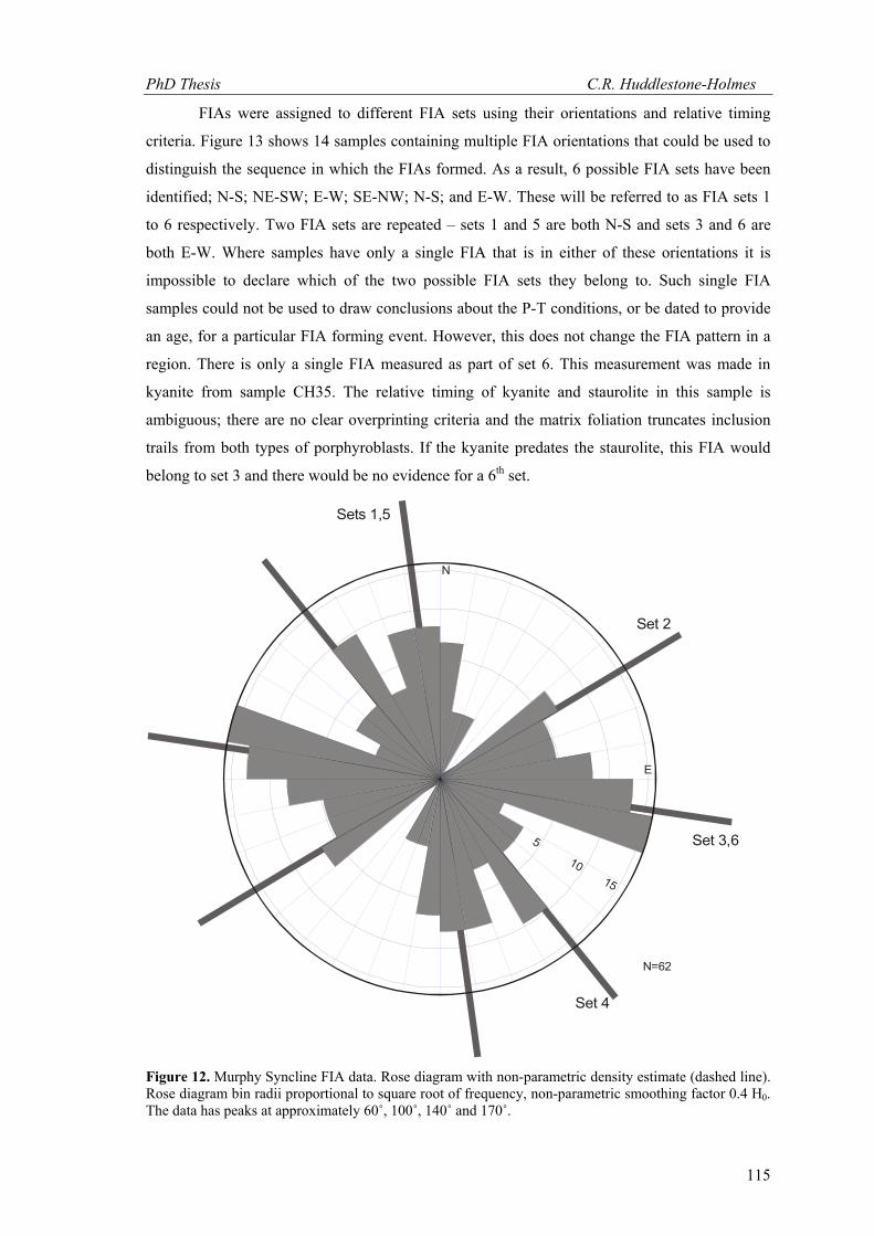
FIAs were assigned to different FIA sets using their orientations and relative timing
criteria. Figure 13 shows 14 samples containing multiple FIA orientations that could be used to
distinguish the sequence in which the FIAs formed. As a result, 6 possible FIA sets have been
identified; N-S; NE-SW; E-W; SE-NW; N-S; and E-W. These will be referred to as FIA sets 1
to 6 respectively. Two FIA sets are repeated – sets 1 and 5 are both N-S and sets 3 and 6 are
both E-W. Where samples have only a single FIA that is in either of these orientations it is
impossible to declare which of the two possible FIA sets they belong to. Such single FIA
samples could not be used to draw conclusions about the P-T conditions, or be dated to provide
an age, for a particular FIA forming event. However, this does not change the FIA pattern in a
region. There is only a single FIA measured as part of set 6. This measurement was made in
kyanite from sample CH35. The relative timing of kyanite and staurolite in this sample is
ambiguous; there are no clear overprinting criteria and the matrix foliation truncates inclusion
trails from both types of porphyroblasts. If the kyanite predates the staurolite, this FIA would
belong to set 3 and there would be no evidence for a 6th set.
Figure 12. Murphy Syncline FIA data. Rose diagram with non-parametric density estimate (dashed line). Rose diagram bin radii proportional to square root of frequency, non-parametric smoothing factor 0.4 H0. The data has peaks at approximately 60˚, 100˚, 140˚ and 170˚.
N
5
1015
E
N=62
Sets 1,5
Set 2
Set 3,6
Set 4
PhD Thesis C.R. Huddlestone-Holmes
116
Figure 13. Distribution of FIAs with errors. Data analysed using the bootstrap MLE approach shown in (a). The error bars show the 95% confidence intervals. The data in (b) are for FIAs determined by the asymmetry method with error bars set at 20˚. Where FIA orientations are near 0˚ or 180˚ they have also been plotted twice, once at the original reading, μ0, and again at μ0 ± 180˚ (so 175˚ becomes -5˚ and 5˚ becomes 185˚). FIA sets 1 through 6 in yellow, orange, blue, green, brown and pink. Colours are combined where no relative timing criteria are present to determine which FIA set an observation belongs to.
0 30 60 90 120 150 180
CH2CH4
CH13CH22CH35CH41CH43CH49CH57CH60CH62CH68CH71CH73
Orientation0 30 60 90 120 150 180
CH2CH7
CH11CH13CH14CH17CH20CH21CH22CH23CH24CH25CH27CH30CH32CH35CH38CH40CH42CH48CH49CH50CH51CH52CH53Ch56CH58CH62CH70CH72
(b)
(a)
PhD Thesis C.R. Huddlestone-Holmes
117
3.2.3 Comparison with Maryland Data Yeh and Bell (2004) measured 221 FIAs in 140 oriented samples collected from the
Baltimore-Washington anticlinorium within the Baltimore terrane of the eastern Maryland
piedmont. They derived a sequence of 8 FIA sets using a similar approach to that applied to the
Murphy Syncline data above. Deformation and metamorphism in the Baltimore terrane
extended from the late Taconic (510 to 460 Ma) through to the early Acadian (408 to 360 Ma`;
Yeh & Bell 2004 and references therein). This is a similar time period to that suggested by
Connelly and Dallmeyer (1993) for metamorphism in the Murphy Syncline. If the assumption
that FIAs represent the direction of bulk shortening within an orogenic belt at a given point in
time is correct, then if the Baltimore and Murphy regions were undergoing deformation and
metamorphism contemporaneously, their FIA progressions should be the same.
The progression of FIA sets derived from the Murphy region data is strikingly similar to
that from the Baltimore region. The exception is that FIA set 1 from the Baltimore region is not
represented in the Murphy data. Set 1 from the Murphy region correlates with sets 2 and 3 from
the Baltimore region although they are recorded in too few samples to be separated. Sets 2, 3, 4
and 5 from the Murphy region correlate with sets 4,5, 6 and 7 from the Baltimore region
respectively. These FIA sets are the most strongly represented in the Murphy region data and
the correlation between the two regions is remarkable. As mentioned above, there may or may
not be a 6th FIA set in the Murphy region data. If this FIA set does exist, it correlates with set 8
from the Baltimore region.
The correlation of FIA sets between the Murphy Syncline and the Baltimore-
Washington anticlinorium provides strong evidence that these two regions underwent similar
deformation histories. Recent EPMA age dating of monazite from the Murphy Syncline yield
ages at both 450 Ma and 400 Ma (pers comm. Lisowiec 2005`; Kohn & Malloy 2004). This also
supports the hypothesis that FIAs represent the direction of relative motion of tectonic plates;
these regions are over 750 km apart and it is hard to imagine circumstances where identical FIA
progressions could be developed by anything other than plate scale processes.
3.3 Detailed Studies – FIAs Across a Fold Another possible application of FIA data is in detailed studies where their orientations
are compared to constrain age dates or deformation processes such as folding, or the rotational
behaviour of porphyroblasts. An example of this was presented by Timms (2003) who did a
study of matrix foliations and inclusion trails in garnet porphyroblasts preserved in a hand-
sample-scale fold. The study included a comparison of the FIAs in each limb of the fold to
make some inferences about fold forming processes and the porphyroblast rotation problem.
The only measure of confidence he gives for the FIA measurements is the range over which
both asymmetries are observed. The bootstrap MLE approach was applied to some of the data in
PhD Thesis C.R. Huddlestone-Holmes
118
Timms (2003) to demonstrate how such a study can benefit from a technique that allows
confidence intervals to be given to FIA measurements.
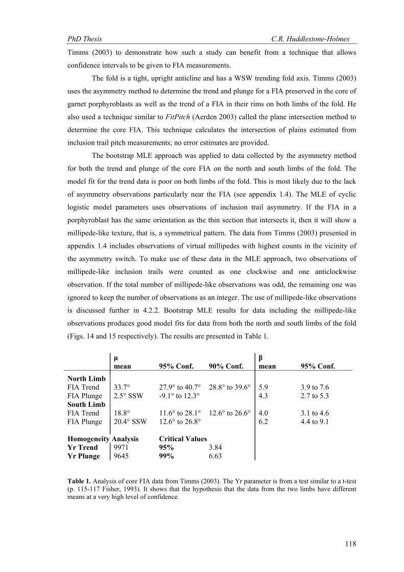
The fold is a tight, upright anticline and has a WSW trending fold axis. Timms (2003)
uses the asymmetry method to determine the trend and plunge for a FIA preserved in the core of
garnet porphyroblasts as well as the trend of a FIA in their rims on both limbs of the fold. He
also used a technique similar to FitPitch (Aerden 2003) called the plane intersection method to
determine the core FIA. This technique calculates the intersection of plains estimated from
inclusion trail pitch measurements; no error estimates are provided.
The bootstrap MLE approach was applied to data collected by the asymmetry method
for both the trend and plunge of the core FIA on the north and south limbs of the fold. The
model fit for the trend data is poor on both limbs of the fold. This is most likely due to the lack
of asymmetry observations particularly near the FIA (see appendix 1.4). The MLE of cyclic
logistic model parameters uses observations of inclusion trail asymmetry. If the FIA in a
porphyroblast has the same orientation as the thin section that intersects it, then it will show a
millipede-like texture, that is, a symmetrical pattern. The data from Timms (2003) presented in
appendix 1.4 includes observations of virtual millipedes with highest counts in the vicinity of
the asymmetry switch. To make use of these data in the MLE approach, two observations of
millipede-like inclusion trails were counted as one clockwise and one anticlockwise
observation. If the total number of millipede-like observations was odd, the remaining one was
ignored to keep the number of observations as an integer. The use of millipede-like observations
is discussed further in 4.2.2. Bootstrap MLE results for data including the millipede-like
observations produces good model fits for data from both the north and south limbs of the fold
(Figs. 14 and 15 respectively). The results are presented in Table 1.
μ β mean 95% Conf. 90% Conf. mean 95% Conf.
North Limb FIA Trend 33.7° 27.9° to 40.7° 28.8° to 39.6° 5.9 3.9 to 7.6 FIA Plunge 2.5° SSW -9.1° to 12.3° 4.3 2.7 to 5.3 South Limb FIA Trend 18.8° 11.6° to 28.1° 12.6° to 26.6° 4.0 3.1 to 4.6 FIA Plunge 20.4° SSW 12.6° to 26.8° 6.2 4.4 to 9.1 Homogeneity Analysis Critical Values Yr Trend 9971 95% 3.84 Yr Plunge 9645 99% 6.63
Table 1. Analysis of core FIA data from Timms (2003). The Yr parameter is from a test similar to a t-test (p. 115-117 Fisher, 1993). It shows that the hypothesis that the data from the two limbs have different means at a very high level of confidence.

PhD Thesis C.R. Huddlestone-Holmes
119
Figure 14. Bootstrap MLE applied to North limb FIA from Timms (2003). The trend is in (a) and the plunge is in (b). Plunges are to the SSW (negative plunges are to the NNE). Millipede-like data included.
10 20 30 40 500.00
0.02
0.04
0.06
0.08
0.10
Deviance
0 5 10 15 200.00
0.02
0.04
0.06
0.08
0.10
0 5 10 15 200.00
0.05
0.10
0.15
0.20re
lativ
efre
quen
cy
Section Orientation
0 30 60 90 120
150
180
Pro
babi
lity
0.00
0.25
0.50
0.75
1.00
Section Orientation
0 30 60 90 120
150
180
0.0
0.5
1.0
1.5
2.0
2.5
3.0
(a)
-200 -150 -100 -50 0 500.0
0.1
0.2
0.3
0.4
Deviance
0 10 20 30 400.00
0.05
0.10
-5 0 5 100.00
0.05
0.10
0.15
0.20
rela
tive
frequ
ency
Section Orientation
-90
-60
-30 0 30 60 90
Prob
abili
ty
0.00
0.25
0.50
0.75
1.00
Section Orientation
-90
-60
-30 0 30 60 90
0.0
0.5
1.0
1.5
2.0
2.5
3.0
(b)
PhD Thesis C.R. Huddlestone-Holmes
112
Figure 10. Reinterpreted FIA data from Stallard et al. (2003). A rose diagram with non-parametric density estimate (dashed line) for the whole dataset is shown in (a). The non-parametric density estimate is a similar approach to the moving averages used by Yeh and Bell (2004). Rose diagram bin radii proportional to square root of frequency. Non-parametric smoothing factor 0.6 H0.The NE -SW, SE-NW and E-W FIA sets are shown in (b).
density estimate (Fisher 1993) in Figure. 10. This is similar to the weighted average approach
used by Yeh (2003) and Yeh and Bell (2004) and is preferred to rose diagrams which can be
distorted by the selection of cell boundaries (Fisher 1993). A U2 test, as described by Bell et al.
(1998), confirms that the data is non-random with a value of 0.857; this is significantly higher
than the critical value at the 95% confidence level of 0.187, which mean the hypothesis that the
Set A
Set 1
Set 3
Set 2
N = 60
N
5
1015
E
N = 25
N
E
10
20
Set 2Set 1 Set 3
a
b
N = 7
N
E
10
2030
N = 27
N
E
10
PhD Thesis C.R. Huddlestone-Holmes
120
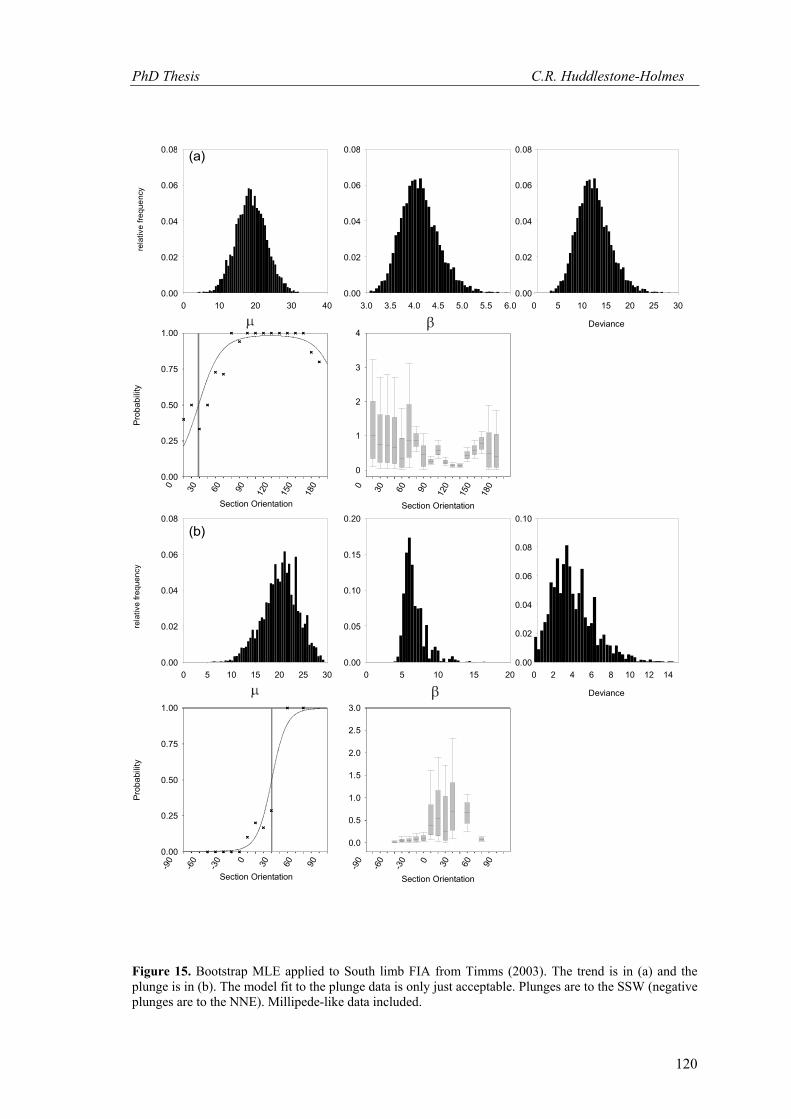
Figure 15. Bootstrap MLE applied to South limb FIA from Timms (2003). The trend is in (a) and the plunge is in (b). The model fit to the plunge data is only just acceptable. Plunges are to the SSW (negative plunges are to the NNE). Millipede-like data included.
0 10 20 30 400.00
0.02
0.04
0.06
0.08
Deviance
0 5 10 15 20 25 300.00
0.02
0.04
0.06
0.08
3.0 3.5 4.0 4.5 5.0 5.5 6.00.00
0.02
0.04
0.06
0.08re
lativ
efre
quen
cy
Section Orientation
0 30 60 90 120
150
180
Pro
babi
lity
0.00
0.25
0.50
0.75
1.00
Section Orientation
0 30 60 90 120
150
180
0
1
2
3
4
(a)
0 5 10 15 20 25 300.00
0.02
0.04
0.06
0.08
Deviance
0 2 4 6 8 10 12 140.00
0.02
0.04
0.06
0.08
0.10
0 5 10 15 200.00
0.05
0.10
0.15
0.20
rela
tive
frequ
ency
Section Orientation
-90
-60
-30 0 30 60 90
Prob
abili
ty
0.00
0.25
0.50
0.75
1.00
Section Orientation
-90
-60
-30 0 30 60 90
0.0
0.5
1.0
1.5
2.0
2.5
3.0
(b)
PhD Thesis C.R. Huddlestone-Holmes
121
The confidence intervals derived for the trends of the FIAs on the two limbs of the fold
overlap slightly at the 95% confidence level. The plunges do not overlap at this confidence
level. A test for homogeneity, called the Yr test (Fisher 1993), which is similar to a t-test used
for linear data, shows that the mean orientations of both the trends and plunges on each side of
the fold differ from each other at even the 99% confidence level (Table. 1). These results
confirm that the FIA orientations differ across the limbs of the fold to a high level of certainty.
Timms (2003) does not provide error estimates for the FIAs calculated using the plane
intersection method. Considering that the standard deviations given for the best fit poles to the
estimated planes are in the order of 15°, the 95% confidence interval in the intersection of the
planes (i.e. the FIA) will be correspondingly large. It is important in drawing conclusions from
such data that the level of confidence that can be placed in the conclusions is considered. The
MLE approach described here makes it possible to test hypotheses about the relationship
between FIA orientations with some statistical certainty.
4 Discussion and Conclusions
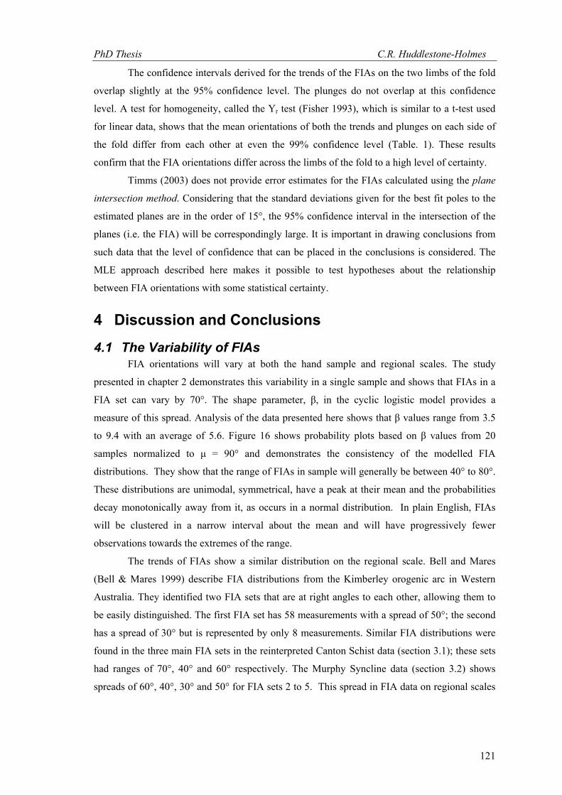
4.1 The Variability of FIAs FIA orientations will vary at both the hand sample and regional scales. The study
presented in chapter 2 demonstrates this variability in a single sample and shows that FIAs in a
FIA set can vary by 70°. The shape parameter, β, in the cyclic logistic model provides a
measure of this spread. Analysis of the data presented here shows that β values range from 3.5
to 9.4 with an average of 5.6. Figure 16 shows probability plots based on β values from 20
samples normalized to μ = 90° and demonstrates the consistency of the modelled FIA
distributions. They show that the range of FIAs in sample will generally be between 40° to 80°.
These distributions are unimodal, symmetrical, have a peak at their mean and the probabilities
decay monotonically away from it, as occurs in a normal distribution. In plain English, FIAs
will be clustered in a narrow interval about the mean and will have progressively fewer
observations towards the extremes of the range.
The trends of FIAs show a similar distribution on the regional scale. Bell and Mares
(Bell & Mares 1999) describe FIA distributions from the Kimberley orogenic arc in Western
Australia. They identified two FIA sets that are at right angles to each other, allowing them to
be easily distinguished. The first FIA set has 58 measurements with a spread of 50°; the second
has a spread of 30° but is represented by only 8 measurements. Similar FIA distributions were
found in the three main FIA sets in the reinterpreted Canton Schist data (section 3.1); these sets
had ranges of 70°, 40° and 60° respectively. The Murphy Syncline data (section 3.2) shows
spreads of 60°, 40°, 30° and 50° for FIA sets 2 to 5. This spread in FIA data on regional scales
PhD Thesis C.R. Huddlestone-Holmes
122
Figure 16. FIA distributions from real samples. This plot shows the FIA distributions from 20 samples analysed from Vermont, New Hampshire and North Carolina, normalized to a FIA orientation of 90˚.
is typical of all results in the literature published to date (e.g. Bell et al. 1998, Cihan & Parsons
2005, Sayab 2005, Yeh & Bell 2004). It could be argued that these distributions are an artefact
because most studies of FIA data use orientation to group the data. However, distributions of
this size are also found where FIA sets lie at high angles to each other (e.g. Bell & Mares 1999,
Sayab 2005) and when relative timing criteria allow them to be clearly differentiated (e.g. Bell
et al. 1998, Yeh & Bell 2004). The shapes of regional FIA distributions are generally the same
as those within a sample, approximating a normal distribution.
The distribution of FIAs at hand sample scale is very similar to that observed at regional
scales. If porphyroblast rotation were a common process, it would be difficult to imagine the
circumstances where such consistent FIA groupings would form, especially in multi-FIA
samples. These distributions suggest that the variation in FIA orientations is related to variations
in the foliations that form them and is consistent with a non-rotational model. The literature
does not provide an adequate discussion of the variability of foliations at any scale. While the
processes that may cause the orientation of a foliation to vary (described in section 1.2) have
been addressed in the literature, no study has linked these processes to hand sample and regional
Section
0 30 60 90 120 150 180
Pro
babi
lity
0.0
0.1
0.2
0.3
0.4
0.5
0.6
0.7
0.8
0.9
1.0
PhD Thesis C.R. Huddlestone-Holmes
123
scale variations. This gap in knowledge is begging to be filled. The distribution of FIAs may
actually provide us with a hypothesis to test – that is, that foliations formed in a single event
vary in orientation by up to 70° on all scales.
The conclusions of Stallard et al. (2003) that FIA orientations can vary by up to 140°
was based on the flawed approach of correlating FIAs between samples using microstructural
textures. Unfortunately their conclusions have been used by at least one author to question the
significance of FIA measurements (Vernon 2004). The consistent results obtained here and in
other FIA studies demonstrate that large variations in FIA orientations within a set do not occur.
4.2 The Collection and Use of FIA Data FIA studies to date contain no indication of any kind of minimum standard for the
measurement and presentation of data. This lack of standards is the case for most structural
data; for example, there is no standard for presenting fold axes measured in an area. This raises
the following questions: should a shape analysis based on eigenvalues be used (Woodcock
1977); or is a stereonet enough, and, if so, should equal angle or equal area be used? It seems
that the geological community is not critical of how such data is presented. FIAs, on the other
hand, are not measured directly and the concept that they remain consistently oriented in spite
of the overprinting effects of younger deformations is difficult for many to accept. The
following section explores the best practice for determining and reporting FIA data.
4.2.1 Comparison of FIA Measurement Techniques The two basic techniques for measuring FIAs are the asymmetry and the FitPitch
methods. The most commonly used asymmetry method uses the asymmetry of curved inclusion
trails to define the trend of a FIA. The FitPitch method measures FIAs by first finding the
orientations of planar foliations that result in straight inclusion trails in thin section and by then
calculating their intersection. The plane intersection method used by Timms (2003) is similar to
the FitPitch except that it relies on the user determining which pitches should be grouped
together to define a particular foliation. FitPitch determines fits of one, two or three model
planes to the pitch data and provides parameters that help to assess which model planes best fit
the data. Comparison studies of the FitPitch and asymmetry methods produce comparable
results (Timms 2003`; unpublished data, Bruce, 2005).
To use the asymmetry method, inclusion trails must exhibit some curvature. If the
inclusion trails are straight, the FitPitch and plane intersection methods can be used. The
advantage of the asymmetry method is that a confidence interval can be assigned to FIA
measurements using the bootstrapped MLE approach. FitPitch does not provide a measure of
error for its FIA estimates and neither does the plane intersection method as applied by Timms
(2003). Because the plane intersection method is based on the intersection of two planes fitted
PhD Thesis C.R. Huddlestone-Holmes
124
to pitch data, error estimates for the orientation of these planes could be propagated to
determine the error of a FIA measured this way.
Both of these approaches for finding FIAs require a minimum amount of data to get
meaningful results. For the asymmetry method, samples where the number of observations in
each thin section is less than ten should be treated with caution, particularly within a 60°
interval centred on the point at which the asymmetries flip. It is likely that a similar number of
observations would be required for the FitPitch approach.
4.2.2 Using “Millipedes” with the Bootstrapped MLE Appraoch The asymmetry method relies on the fact that the intersection of a curved inclusion trail
in thin section will either be clockwise or anticlockwise. The FIA lies at the point at which the
probability of observing a particular geometry (e.g. clockwise), is half. A third possible
geometry that may be observed in thin sections that are parallel to the FIA are millipede-like
inclusion trail geometries. The term millipede was first used by Rubenach and Bell (1980) to
describe inclusion trails that form as the result of coaxial deformation. True millipede trails
display no asymmetry regardless of the orientation they are intersected at. Millipede-like refers
to the case when inclusion trails that appear to be millipedes are observed as the result of a cut
effect (Bell and Bruce, pers. comm., 2005). These features will be observed when curved
inclusion trails are intersected by a thin section cut parallel to their axis of curvature (e.g fig
4.d,f in Stallard et al. 2002).
The occurrence of millipede-like geometries is used in the asymmetry method as an
indication that the thin section containing them lies close to the orientation of the FIA. These
observations can be important in examples where the number of porphyroblasts with clear
asymmetries is low in sections oriented near the FIA. The data from Timms (2003) examined in
section 3.3 is a good example of this (appendix 1.4). The bootstrapped MLE approach is based
on a logistic model which looks at the probability of a success (clockwise observation) or a
failure (anticlockwise observation). To include millipede-like observations they need to be
reclassified as one of these two options. The recommended approach is to count each two
millipede-like observations as one clockwise and one anticlockwise observation. If there were
an odd number of observations the last is ignored to keep the number of observations as an
integer. Millipede-like data push the observed probability of a success towards 0.5 when used in
this way. The effect of counting a millipede-like observation as both one clockwise and one
anticlockwise observation is to weight them as two observations, which would bias the results.
Before using millipede-like inclusion trails in the asymmetry method, it is imperative
that the user is certain that they are not true millipedes. If millipede textures are observed in all
section orientations in a sample then they most likely are true millipedes and should not be used.
Collecting sufficient asymmetry observations so that millipede-like observations do not have to
PhD Thesis C.R. Huddlestone-Holmes
125
be used would avoid this issue altogether. Other types of inclusion trail geometries, such as
straight or shotgun patterns cannot be interpreted as having a geometry related to the FIA
orientation and are of no value in determining FIAs using the asymmetry method.
4.2.3 Detailed Studies FIAs provide a potential marker that can be used as a reference frame both within and
between samples. When used in this way, it is important that potential errors in the orientation
of FIA measurements are given. The analysis of the core FIA data from Timms (2003) in
section 3.3 demonstrates how inferences made based on FIA data can be strengthened when the
confidence in a FIA measurement is provided. The bootstrapped MLE approach provides a
technique whereby confidence intervals of a FIA measurement can be readily determined. It
also helps the recognition of samples where FIAs may be from a mixed or randomly distributed
population, and where the number of observations is insufficient to have confidence in a FIA
measurement.
Another example of where the bootstrapped MLE approach would have been of benefit
appears in a paper on dating of FIAs by Bell and Welch (2002). They used EPMA age dating of
monazite to constrain the timing of FIA formation in several samples from Vermont. This
involved correlating FIAs between sample and within a regional data set. The strength of such
correlations may be called into question unless the confidence intervals for the orientations of
the FIAs in each sample are given, as they are for the age dates.
As well as reporting the orientations for FIAs, shape parameters (β) and their
confidence intervals, the raw asymmetry counts, the number of bootstraps, the bootstrap
technique used, and plots of the distributions of μ, β and the sample deviance should also be
included when reporting the results of detailed studies. Any relative timing criteria should also
be described. Providing the information allows the reader to confirm the goodness-of-fit of the
proposed model parameters and to re-evaluate the data as they see fit. Techniques such as
FitPitch or the plane intersection method should only be used for detailed studies if errors for
the determined FIA orientations are calculated.
4.2.4 Regional Studies Regional FIA studies are concerned with the distribution and relative timing of FIA sets
for the region as a whole rather than within individual samples. Any error in individual
measurements will be accommodated within the distribution of FIAs in a set if a sufficiently
large number of measurements have been made. The number of FIA measurements required
would depend on the number and distribution of FIA sets in the region, so the minimum sample
size will vary. Descriptive statistical techniques for circular data, such as those outlined in
Fisher (1993) or Mardia and Jupp (2000), can be applied. These methods would allow the
inferences based on the distributions of FIA sets to be made with proper statistical rigour.
PhD Thesis C.R. Huddlestone-Holmes
126
A key component of the analysis of regional datasets is the determination of FIA sets.
There are three components to this: defining the trends of FIA sets; deciding which
measurements belong in each set; and determining the relative timing of FIA sets. Graphical
techniques such as the weighted average approach used by Yeh and Bell (2004) or the non-
parametric density estimate used here provide a means of identifying peaks in the whole data
set. The non-parametric density estimate, which was recommended by Fisher (1993), provides a
way of exploratory analysis of circular data. It is comparable to a weighted average and allows
data to be examined without the bias that may be present in a rose diagram due to the location of
bin boundaries. A parametric density estimate is similar to the moving average used by Yeh and
Bell (2004) and has the advantage of avoiding the issues that arise in presenting circular data on
a linear plot. Once these peaks are identified the individual FIA measurements can be assigned
to FIA sets based on their orientation. It is important to emphasize the point that using inclusion
trail textures is a totally unreliable approach due to the effects of deformation partitioning.
The order in which the FIA sets formed can be determined using relative timing criteria
once the orientations of FIA sets have are identified. Relative timing criteria can only be applied
within samples. Applying these criteria between samples makes too great an assumption on the
pervasiveness of deformation and metamorphism. The are only two reliable relative timing
criteria; where two or more FIAs with different orientations are found in individual
porphyroblasts; and where different FIAs are preserved in different porphyroblastic phases with
clear overprinting relationships. Absolute timing using in situ age dating could also be used,
although this would be impractical for large datasets. In some cases relative timing criteria may
reveal FIA sets that overlap or are repeated, such as in the Murphy Syncline data described in
section 3.2.2. It is not possible to assign a FIA measurement to one of these sets for single FIA
samples when overlap or repitition occurs.
The bootstrapped MLE approach would provide little additional information for large
regional datasets. There may be some value in analysing a group of representative samples from
the region to characterize the typical intra sample FIA distributions. This scrutiny may prove
critical when trying to assign a FIA measurement to a given FIA set. It is also recommended
that the bootstrap MLE approach be applied when a sample is being used to determine a FIA
set’s age or the P-T conditions it formed under. This approach provides some certainty that the
data from that sample does have an orientation that matches the FIA set in question.
4.3 The Significance of FIAs FIAs preserve the fabrics formed by the deformation events that were active at the time
the porphyroblasts grew. Importantly, they preserve the orientation of these fabrics through
subsequent deformation events that reorient or destroy the equivalent fabrics in the matrix. FIAs
are analogous to the intersection lineation between subsequent foliations. Their significance is
PhD Thesis C.R. Huddlestone-Holmes
127
similar to that of intersection lineations with the distinction that they will not have been
reoriented by subsequent deformation events. The consistent distribution of FIAs within
samples together with the fact that they can easily be grouped as FIA sets suggest that any
reorientation of FIAs by rotation of porphyroblasts relative to each other is insignificant.
Because foliations typically form in sub-horizontal and sub-vertical orientations (Bell &
Johnson 1989, Bell & Newman 2006), FIA trends will reflect the orientation of the sub-vertical
foliations that formed them. If foliations form perpendicular to the direction of bulk shortening,
so will FIAs. A FIA set can represent a number of foliation forming events, so it is
representative of a time period when the direction of horizontal bulk shortening was relatively
constant. FIA sets can be correlated between samples or between regions providing a more
detailed history of the deformation than is possible by using macro-scale structures or matrix
microstructures. This history provides a reference frame in which age dates and P-T paths can
be placed.
FIA data have been applied to many geological problems: investigating tectono-
metamorphic histories and correlating multiple phases of metamorphism on local and orogenic
scales (e.g. Bell et al. 2005, Bell et al. 1998, Bell & Mares 1999, Cihan & Parsons 2005, Lee et
al. 2000, Sayab 2005, Yeh & Bell 2004); investigating foliation development and folding
mechanisms (Bell & Hickey 1997, Timms 2003); arguing for the lack of porphyroblast rotation
(Bell et al. 1997, Ham & Bell 2004, Hickey & Bell 1999); studying porphyroblast nucleation
and growth relative to deformation (Bell et al. 2003, Bell et al. 2004); reconstructing plate
motions (Bell et al. 1995); constraining age dates (Bell & Welch 2002); defining complex
deformation partitioning patterns (Bell et al. 2004); and investigating pluton emplacement
mechanisms and timing (Davis 1993). The analytical techniques recommended here will
enhance future applications of FIA data by ensuring that the interpretations are statistically
valid.
References Aerden, D. 2003. Preferred orientation of planar microstructures determined via statistical best-
fit of measured intersection-lines: the 'FitPitch' computer program. Journal of Structural Geology 25(6), 923-934.
Aerden, D. 2004. Correlating deformation in Variscan NW-Iberia using porphyroblasts; implications for the Ibero-Armorican Arc. Journal of Structural Geology 26(1), 177-196.
Aerden, D. G. A. M. 1995. Porphyroblast non-rotation during crustal extension in the Variscan Lys-Caillaouas Massif, Pyrenees. Journal of Structural Geology 17, 709-725.
Beirmeier, C. & Stuwe, K. 2003. Strain rates from snowball garnet. Journal of Metamorphic Geology 21, 253-268.
Bell, T. H. 1978. The development of slaty cleavage across the Nackara Arc of the Adelaide Geosyncline. Tectonophysics 51(3-4), 171-174.
Bell, T. H. 1986. Foliation development and reactivation in metamorphic rocks: the reactivation of earlier foliations and decrenulation due to shifting patterns of deformation partitioning. Journal of Metamorphic Geology 4, 421-444.
PhD Thesis C.R. Huddlestone-Holmes
128
Bell, T. H. & Chen, A. 2002. The development of spiral-shaped inclusion trails during multiple metamorphism and folding. Journal of Metamorphic Geology 20(4), 397 -412.
Bell, T. H. & Duncan, A. C. 1978. A rationalized and unified shorthand terminology for lineations and fold axes in tectonites. Tectonophysics 47(1-2), T1-T5.
Bell, T. H., Forde, A. & Hayward, N. 1992. Do smoothly-curving spiral shaped inclusion trails signify porphyroblast rotation? Geology 20, 59-62.
Bell, T. H., Forde, A. & Wang, J. 1995. A new indicator of movement direction during orogenesis: measurement technique and application to the Alps. Terra Nova V. 7, 500-508.
Bell, T. H., Ham, A. P., Hayward, N. & Hickey, K. A. 2005. On the development of gneiss domes. Australian Journal of Earth Sciences 42(2), in press.
Bell, T. H., Ham, A. P. & Hickey, K. A. 2003. Early formed regional antiforms and synforms that fold younger matrix schistosities: their effect on sites of mineral growth. Tectonophysics 367(3-4), 253 -278.
Bell, T. H., Ham, A. P. & Kim, H. S. 2004. Partitioning of deformation along an orogen and its effects on porphyroblast growth during orogenesis. Journal of Structural Geology 26(5), 825 -845.
Bell, T. H. & Hayward, N. 1991. Episodic metamorphic reactions during orogenesis; the control of deformation partitioning on reaction sites and reaction duration. Journal of Metamorphic Geology 9(5), 619-640.
Bell, T. H. & Hickey, K. A. 1997. Distribution of pre-folding linear indicators of movement direction around the Spring Hill Synform, Vermont; significance for mechanism of folding in this portion of the Appalachians. Tectonophysics 274(4), 275-294.
Bell, T. H. & Hickey, K. A. 1999. Complex microstructures preserved in rocks with a simple matrix; significance for deformation and metamorphic processes. Journal of Metamorphic Geology 17(5), 521-535.
Bell, T. H., Hickey, K. A. & Upton, G. J. G. 1998. Distinguishing and correlating multiple phases of metamorphism across a multiply deformed region using the axes of spiral, staircase and sigmoidal inclusion trails in garnet. Journal of Metamorphic Geology 16(6), 767-794.
Bell, T. H., Hickey, K. A. & Wang, J. 1997. Spiral and staircase inclusion trail axes within garnet and staurolite porphyroblasts from schists of the Bolton Syncline, Connecticut; timing of porphyroblast growth and the effects of fold development. Journal of Metamorphic Geology 15(4), 467-478.
Bell, T. H. & Johnson, S. E. 1989. Porphyroblast inclusion trails: the key to orogenesis. Journal of Metamorphic Geology 7, 279-310.
Bell, T. H. & Mares, V. M. 1999. Correlating deformation and metamorphism around orogenic arcs. American Mineralogist 84(11-12), 1727 -1740.
Bell, T. H. & Newman, R. 2006. Appalachian orogenesis: the role of repeated gravitational collapse. In: Styles of Continental Compression. Geological Society of America Speacial Paper xxx. (edited by Mazzoli, S. & Butler, R.) In Press. Geological Society of America, Bolder, Colarado.
Bell, T. H. & Rubenach, M. J. 1980. Crenulation cleavage development--evidence for progressive bulk inhomogeneous shortening from "millipede" microstructures in the robertson river metamorphics. Tectonophysics 68(1-2), T9-T15.
Bell, T. H. & Wang, J. 1999. Linear indicators of movement direction (mineral elongation lineations, stretching lineations and slickensides) versus Foliation Intersection Axes in porphyroblasts (FIAs) and their relationships to directions of relative plate motion. Earth Science Frontiers 6, 31-47.
Bell, T. H. & Welch, P. W. 2002. Prolonged Acadian orogenesis: Revelations from foliation intersection axis (FIA) controlled monazite dating of foliations in porphyroblasts and matrix. American Journal of Science 302(7), 549 -581.
Cihan, M. & Parsons, A. 2005. The use of porphyroblasts to resolve the history of macro-scale structures: an example from the Robertson River Metamorphics, North-Eastern Australia. Journal of Structural Geology 27(6), 1027-1045.
PhD Thesis C.R. Huddlestone-Holmes
129
Connelly, J. B. & Dallmeyer, R. D. 1993. Polymetamorphic Evolution of the Western Blue Ridge - Evidence from Ar-40/Ar-39 Whole-Rock Slate/Phyllite and Muscovite Ages. American Journal of Science 293(4), 322-359.
Davis, B. K. 1993. Mechanism of emplacement of the Cannibal Creek Granite with special reference to timing and deformation history of the aureole. Tectonophysics 224, 337-362.
Evins, P. M. 2005. A 3D study of aligned porphyroblast inclusion trails across shear zones and folds. Journal of Structural Geology In Press, Corrected Proof, 1300-1314.
Fisher, N. I. 1993. Statistical analysis of circular data. Cambridge University Press, Cambridge, [England].
Fyson, W. K. 1980. Fold fabrics and emplacement of an Archean granitoid pluton, Cleft Lake, Northwest Territories. Canadian Journal of Earth Science V.17, 325 - 332.
Glover, L., Speer, J. A., Russell, G. S. & Farrar, S. S. 1983. Ages of Regional Metamorphism and Ductile Deformation in the Central and Southern Appalachians. Lithos 16(3), 223-245.
Ham, A. P. & Bell, T. H. 2004. Recycling of foliations during folding. Journal of Structural Geology 26(11), 1989-2009.
Hatcher, R. D. 1987. Tectonics of the Southern and Central Appalachian Internides. Annual Review of Earth and Planetary Sciences 15, 337-362.
Hayward, N. 1990. Determination of early fold axis orientations in multiply deformed rocks using porphyroblast inclusion trails. Tectonophysics V. 179, 353-369.
Hayward, N. 1992. Microstructural analysis of the classical spiral garnet porphyroblasts of South-east Vermont; evidence for non-rotation. Journal of Metamorphic Geology 10(4), 567-587.
Hickey, K. A. & Bell, T. H. 1999. Behaviour of rigid objects during deformation and metamorphism; a test using schists from the Bolton Syncline, Connecticut, USA. Journal of Metamorphic Geology 17(2), 211-228.
Johnson, S. E. 1990. Lack of porphyroblast rotation in the Otago schists, New Zealand: implications for crenulation cleavage development, folding and deformation partitioning. Journal of Metamorphic Geology 8, 13-30.
Johnson, S. E. 1993. Unravelling the spirals: a serial thin-section study and three dimensional computer-aided reconstruction of spiral-shaped inclusion trails in garnet porphyroblasts. Journal of Metamorphic Geology 11, 621-634.
Johnson, S. E. 1999a. Near-orthogonal foliation development in orogens: meaningless complexity, or reflection of fundamental dynamic processes. Journal of Structural Geology 21, 1183-1187.
Johnson, S. E. 1999b. Porphyroblast microstructures: A review of current and future trends. American Mineralogist V.84, 1711-1726.
Jung, W. S., Ree, J. H. & Park, Y. 1999. Non-rotation of garnet porphyroblasts and 3-D inclusion trail data: an example from the Imjingang belt, South Korea. Tectonophysics 307(3-4), 381-395.
Kohn, M. J. & Malloy, M. A. 2004. Formation of monazite via prograde metamorphic reactions among common silicates: implications for age determinations. Geochimica et Cosmochimica Acta 68(1), 101-113.
Lee, H., Lee, B.-J. & Otoh, S. 2000. Significance of systematic changes in crenulation asymmetries within meta-sediments across the Ogcheon Supergroup in the Goesan area, southern Korea. Hanrimwon Publishing Company for the Geological Society of Korea, Seoul, South Korea, 115-134.
Mardia, K. V. & Jupp, P. E. 2000. Directional Statistics. J. Wiley, Chichester, England. Mohr, D. W. 1973. Stratigraphy and Structure of Part of Great Smoky and Murphy Belt Groups,
Western North-Carolina. American Journal of Science A273, 41-71. Powell, D. & Treagus, J. E. 1967. On the geometry of S-shaped inclusion trails in garnet
porphyroblasts. Mineralogical Magazine 36, 453-456. Rodgers, J. 1987. The Appalachian-Ouachita Orogenic Belt. Episodes 10(4), 259-266.

PhD Thesis C.R. Huddlestone-Holmes
130
Rosenfeld, J. L. 1970. Rotated Garnets in Metamorphic Rocks. Geological Society of America Special Paper, 129. Geological Society of America, Boulder, Colarado.
Sayab, M. 2005. Microstructural evidence for N-S shortening in the Mount Isa Inlier (NW Queensland, Australia): the preservation of early W-E-trending foliations in porphyroblasts revealed by independent 3D measurement techniques. Journal of Structural Geology 27(8), 1445-1468.
Stallard, A., Hickey, K. A. & Upton, G. J. G. 2003. Measurement and correlation of microstructures: the case of foliation intersection axes. Journal of Metamorphic Geology 21, 241-252.
Stallard, A., Ikei, H. & Masuda, T. 2002. Numerical simulations of spiral-shaped inclusion trails: can 3D geometry distinguish between end-member models of spiral formation? Journal of Metamorphic Geology 20, 801-812.
Steinhardt, C. 1989. Lack of porphyroblast rotation in noncoaxially deformed schists from Petrel Cove, South Australia, and its implications. Tectonophysics 158, 127-140.
Timms, N. E. 2003. Garnet porphyroblast timing and behaviour during fold evolution: implications from a 3-D geometric analysis of a hand-sample scale fold in a schist. Journal of Metamorphic Geology 21(9), 853-873.
Treagus, S. H. 1983. A new theory of finite strain variation through contrasting layers, and its bearing on cleavage refraction. Journal of Structural Geology 5, 351-358.
Treagus, S. H. 1988. Strain refraction in layered systems. Journal of Structural Geology 10(5), 517-527.
Tull, J. F., Ausich, W. I., Groszos, M. S. & Thompson, T. W. 1993. Appalachian Blue Ridge Cover Sequence Ranges at Least into the Ordovician. Geology 21(3), 215-218.
Unrug, R. & Unrug, S. 1990. Paleontological Evidence of Paleozoic Age for the Walden-Creek Group, Ocoee Supergroup, Tennessee. Geology 18(11), 1041-1045.
Upton, G. J. G., Hickey, K. A. & Stallard, A. 2003. Regression models for cyclic data. Royal Statistical Society Journal. Series C: Applied Statistics. 52(Part 2), 227-235.
Vernon, R. H. 2004. A practical guide to rock microstructure. Cambridge, Cambridge University Press, United Kingdom.
Wiener, L. S. & Merschat, C. E. 1992. Geological map of south-western North Carolina including adjoining south-eastern Tennesseeand Northern Georgia. Division of Land Resources, North Carolina Department of Environment, Health, and Natural Resources.
Woodcock, N. H. 1977. Specification of fabric shapes using an eigenvalue method. Geological Society of America Bulletin 88, 1231-1236.
Yeh, M.-W. 2003. The significance and application of foliation intersection/inflection axes (FIA) within porphyroblasts; a review. Diqiu Kexue Jikan = TAO, Terrestrial, Atmospheric and Oceanic Sciences 14(4), 401-419.
Yeh, M.-W. & Bell, T. H. 2004. Significance of dextral reactivation of an E-W transfer fault in the formation of the Pennsylvania orocline, central Appalachians. Tectonics 23, TC5009, doi:10.1029/2003TC001593.
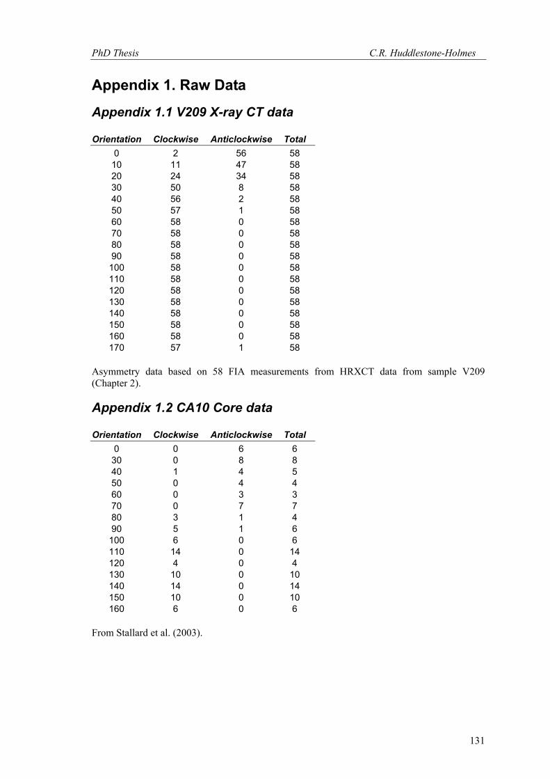
PhD Thesis C.R. Huddlestone-Holmes
131
Appendix 1. Raw Data
Appendix 1.1 V209 X-ray CT data Orientation Clockwise Anticlockwise Total
0 2 56 58 10 11 47 58 20 24 34 58 30 50 8 58 40 56 2 58 50 57 1 58 60 58 0 58 70 58 0 58 80 58 0 58 90 58 0 58 100 58 0 58 110 58 0 58 120 58 0 58 130 58 0 58 140 58 0 58 150 58 0 58 160 58 0 58 170 57 1 58
Asymmetry data based on 58 FIA measurements from HRXCT data from sample V209 (Chapter 2).
Appendix 1.2 CA10 Core data Orientation Clockwise Anticlockwise Total
0 0 6 6 30 0 8 8 40 1 4 5 50 0 4 4 60 0 3 3 70 0 7 7 80 3 1 4 90 5 1 6 100 6 0 6 110 14 0 14 120 4 0 4 130 10 0 10 140 14 0 14 150 10 0 10 160 6 0 6
From Stallard et al. (2003).
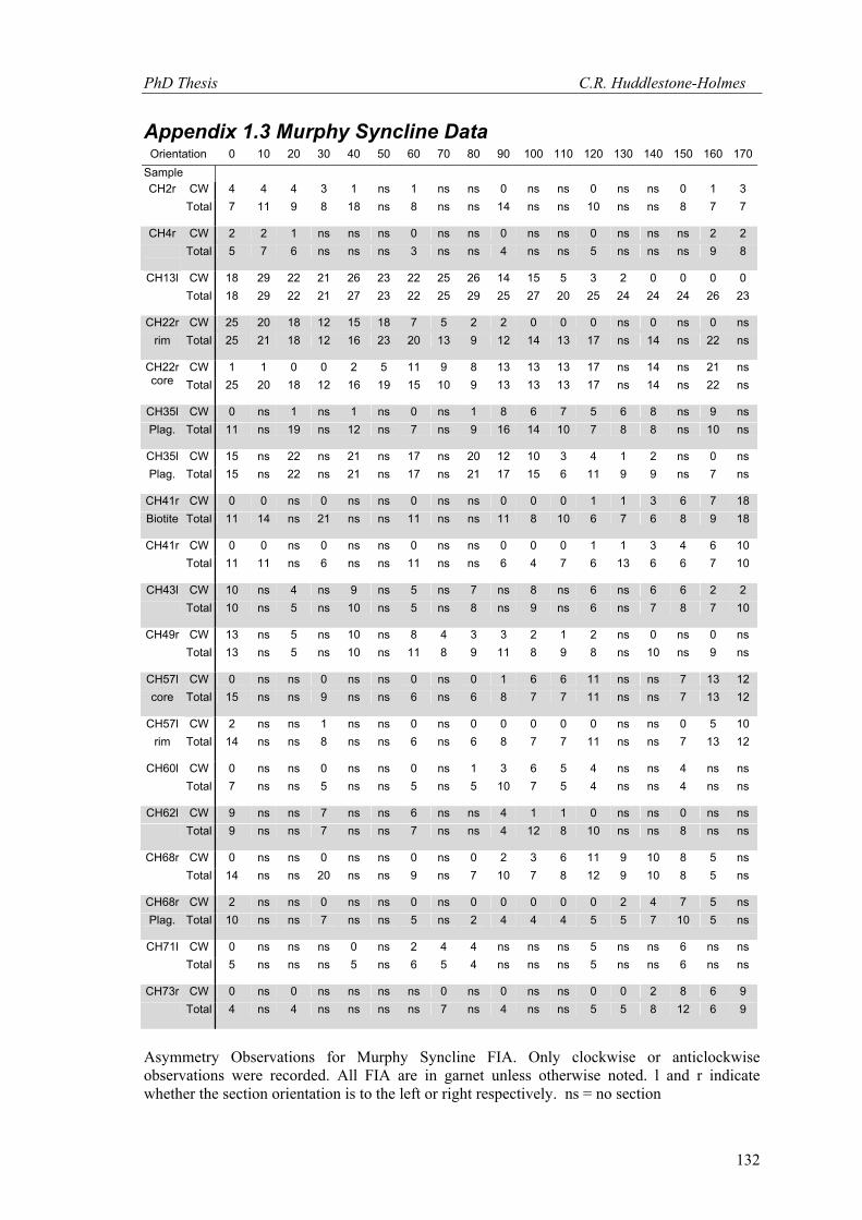
PhD Thesis C.R. Huddlestone-Holmes
132
Appendix 1.3 Murphy Syncline Data Orientation 0 10 20 30 40 50 60 70 80 90 100 110 120 130 140 150 160 170
Sample CH2r CW 4 4 4 3 1 ns 1 ns ns 0 ns ns 0 ns ns 0 1 3
Total 7 11 9 8 18 ns 8 ns ns 14 ns ns 10 ns ns 8 7 7
CH4r CW 2 2 1 ns ns ns 0 ns ns 0 ns ns 0 ns ns ns 2 2
Total 5 7 6 ns ns ns 3 ns ns 4 ns ns 5 ns ns ns 9 8
CH13l CW 18 29 22 21 26 23 22 25 26 14 15 5 3 2 0 0 0 0
Total
18 29 22 21 27 23 22 25 29 25 27 20 25 24 24 24 26 23
CH22r CW 25 20 18 12 15 18 7 5 2 2 0 0 0 ns 0 ns 0 ns rim Total
25 21 18 12 16 23 20 13 9 12 14 13 17 ns 14 ns 22 ns
CW 1 1 0 0 2 5 11 9 8 13 13 13 17 ns 14 ns 21 ns CH22r core
Total
25 20 18 12 16 19 15 10 9 13 13 13 17 ns 14 ns 22 ns
CH35l CW 0 ns 1 ns 1 ns 0 ns 1 8 6 7 5 6 8 ns 9 ns Plag. Total
11 ns 19 ns 12 ns 7 ns 9 16 14 10 7 8 8 ns 10 ns
CH35l CW 15 ns 22 ns 21 ns 17 ns 20 12 10 3 4 1 2 ns 0 ns Plag. Total
15 ns 22 ns 21 ns 17 ns 21 17 15 6 11 9 9 ns 7 ns
CH41r CW 0 0 ns 0 ns ns 0 ns ns 0 0 0 1 1 3 6 7 18 Biotite Total
11 14 ns 21 ns ns 11 ns ns 11 8 10 6 7 6 8 9 18
CH41r CW 0 0 ns 0 ns ns 0 ns ns 0 0 0 1 1 3 4 6 10 Total
11 11 ns 6 ns ns 11 ns ns 6 4 7 6 13 6 6 7 10
CH43l CW 10 ns 4 ns 9 ns 5 ns 7 ns 8 ns 6 ns 6 6 2 2 Total
10 ns 5 ns 10 ns 5 ns 8 ns 9 ns 6 ns 7 8 7 10
CH49r CW 13 ns 5 ns 10 ns 8 4 3 3 2 1 2 ns 0 ns 0 ns Total
13 ns 5 ns 10 ns 11 8 9 11 8 9 8 ns 10 ns 9 ns
CH57l CW 0 ns ns 0 ns ns 0 ns 0 1 6 6 11 ns ns 7 13 12 core Total
15 ns ns 9 ns ns 6 ns 6 8 7 7 11 ns ns 7 13 12
CH57l CW 2 ns ns 1 ns ns 0 ns 0 0 0 0 0 ns ns 0 5 10 rim Total
14 ns ns 8 ns ns 6 ns 6 8 7 7 11 ns ns 7 13 12
CH60l CW 0 ns ns 0 ns ns 0 ns 1 3 6 5 4 ns ns 4 ns ns Total
7 ns ns 5 ns ns 5 ns 5 10 7 5 4 ns ns 4 ns ns
CH62l CW 9 ns ns 7 ns ns 6 ns ns 4 1 1 0 ns ns 0 ns ns Total
9 ns ns 7 ns ns 7 ns ns 4 12 8 10 ns ns 8 ns ns
CW 0 ns ns 0 ns ns 0 ns 0 2 3 6 11 9 10 8 5 ns CH68r Total
14 ns ns 20 ns ns 9 ns 7 10 7 8 12 9 10 8 5 ns
CH68r CW 2 ns ns 0 ns ns 0 ns 0 0 0 0 0 2 4 7 5 ns Plag. Total
10 ns ns 7 ns ns 5 ns 2 4 4 4 5 5 7 10 5 ns
CH71l CW 0 ns ns ns 0 ns 2 4 4 ns ns ns 5 ns ns 6 ns ns Total
5 ns ns ns 5 ns 6 5 4 ns ns ns 5 ns ns 6 ns ns
CH73r CW 0 ns 0 ns ns ns ns 0 ns 0 ns ns 0 0 2 8 6 9 Total
4 ns 4 ns ns ns ns 7 ns 4 ns ns 5 5 8 12 6 9
Asymmetry Observations for Murphy Syncline FIA. Only clockwise or anticlockwise observations were recorded. All FIA are in garnet unless otherwise noted. l and r indicate whether the section orientation is to the left or right respectively. ns = no section
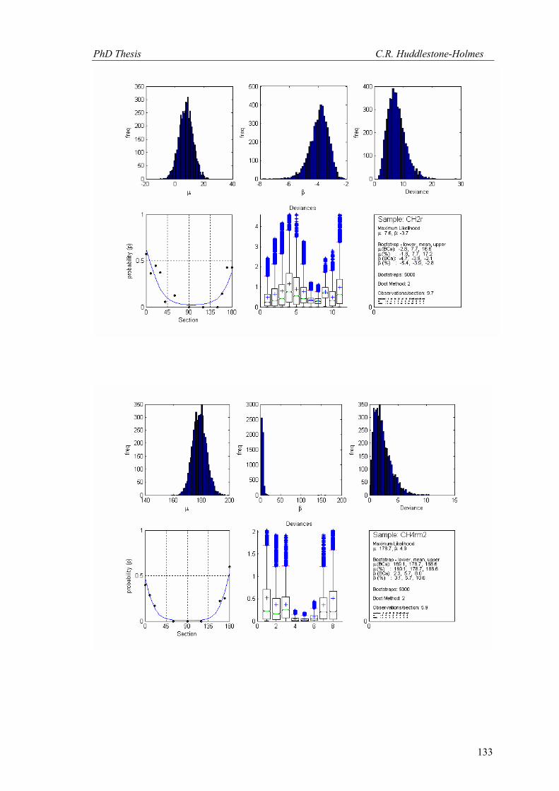
PhD Thesis C.R. Huddlestone-Holmes
133
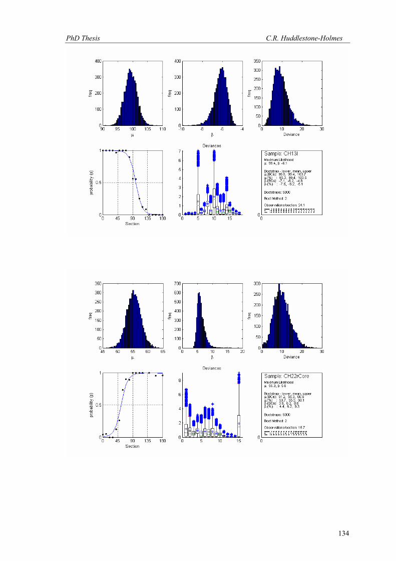
PhD Thesis C.R. Huddlestone-Holmes
134
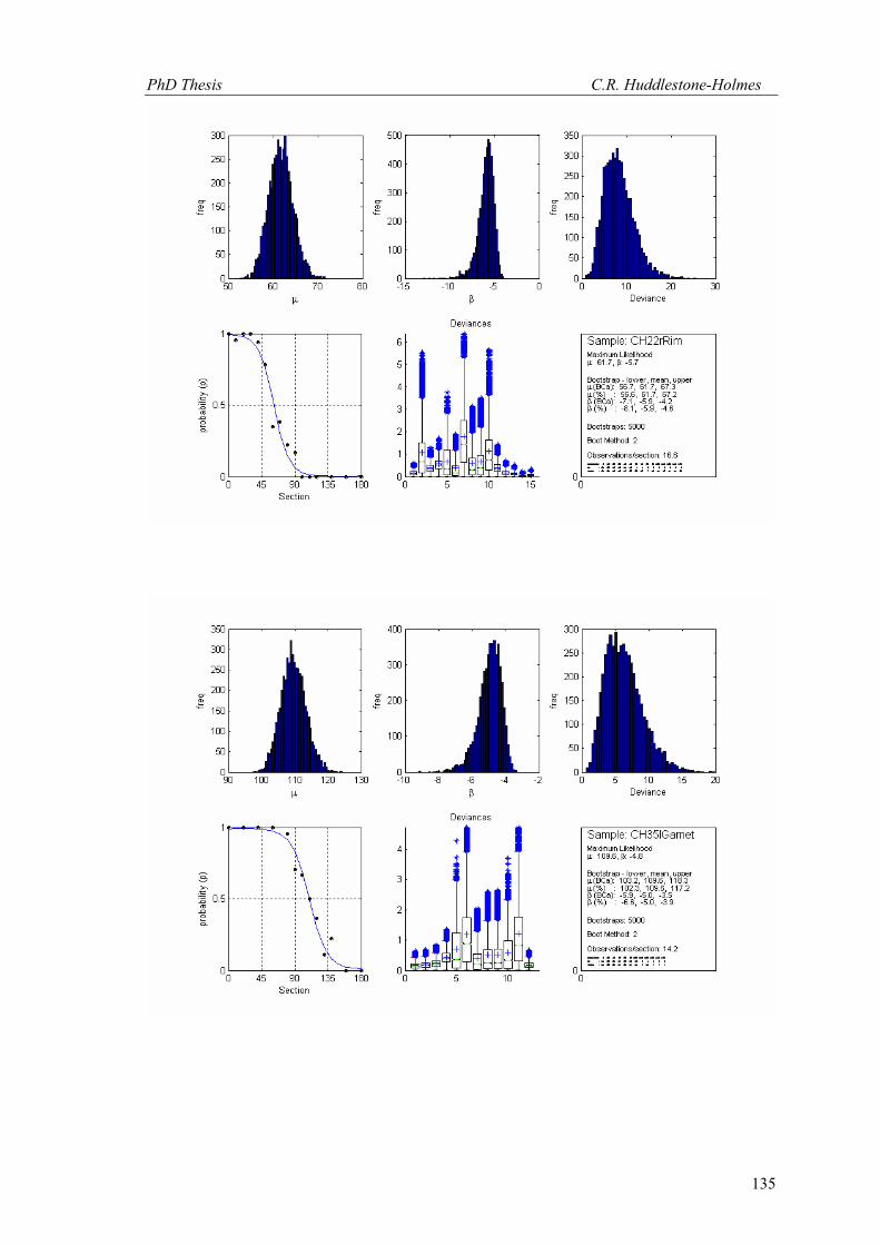
PhD Thesis C.R. Huddlestone-Holmes
135
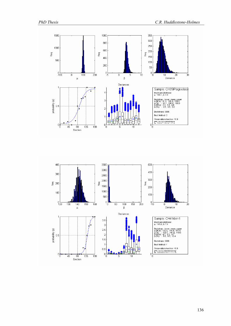
PhD Thesis C.R. Huddlestone-Holmes
136
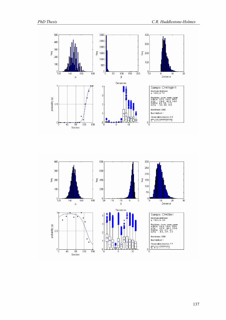
PhD Thesis C.R. Huddlestone-Holmes
137
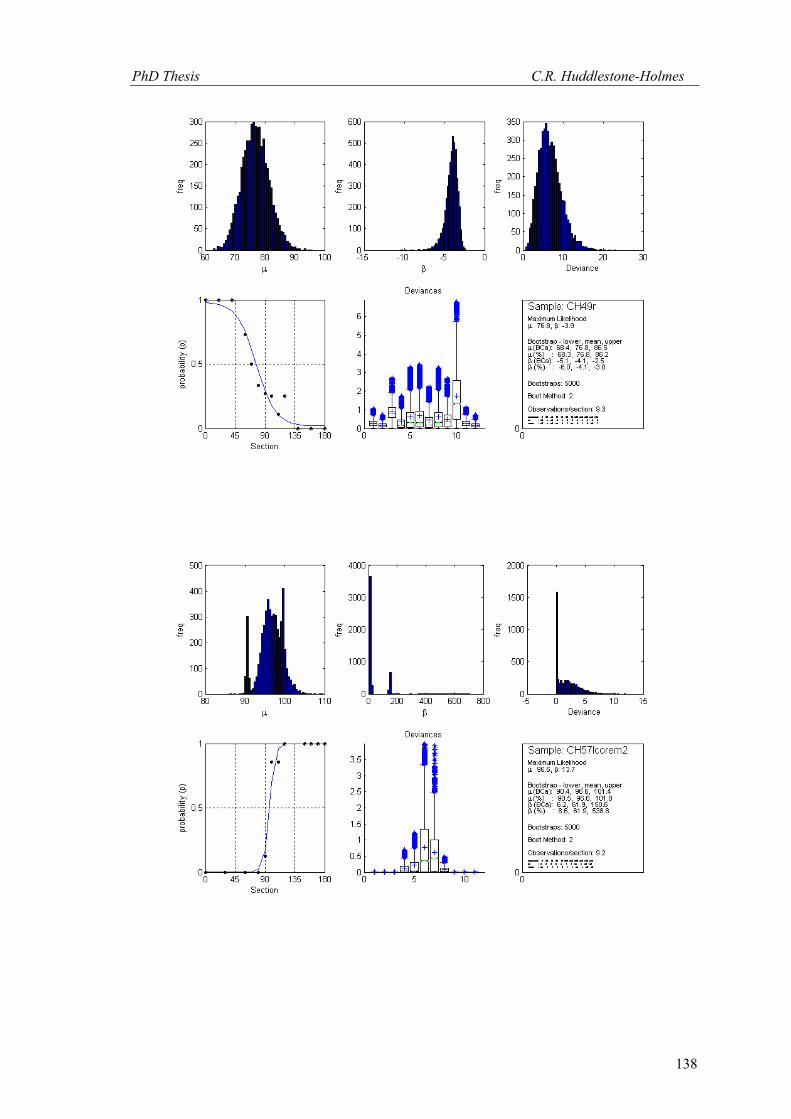
PhD Thesis C.R. Huddlestone-Holmes
138
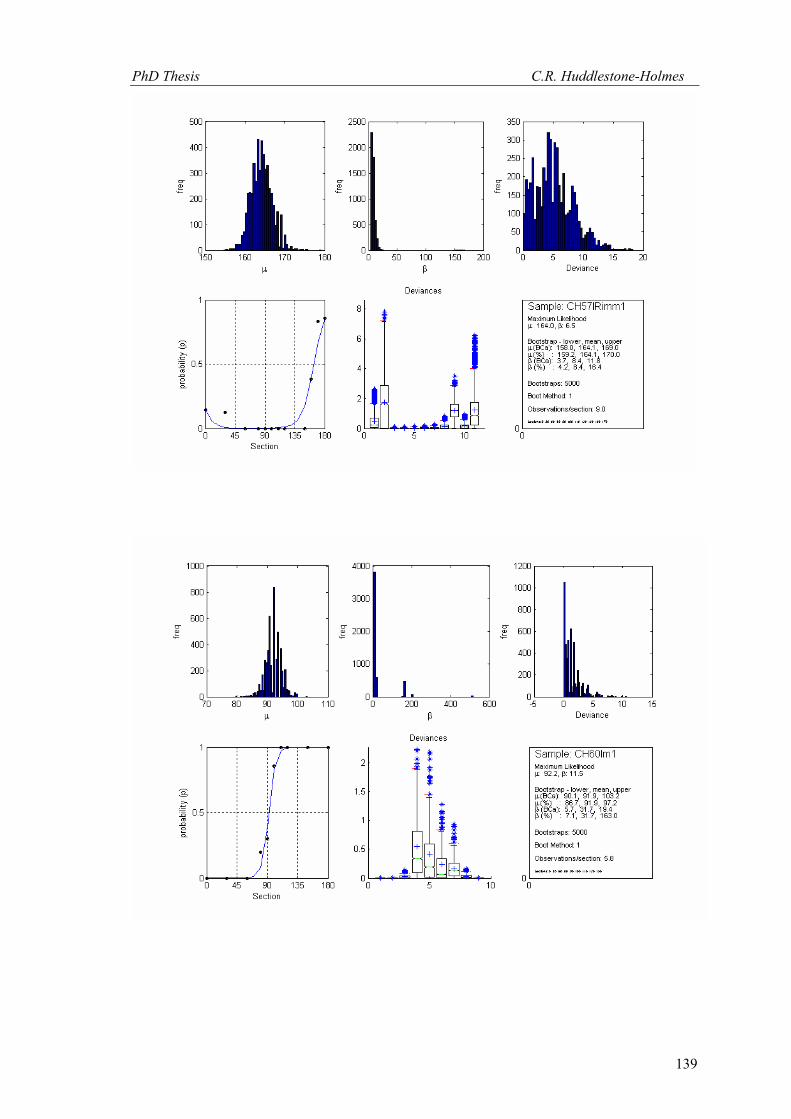
PhD Thesis C.R. Huddlestone-Holmes
139
PhD Thesis C.R. Huddlestone-Holmes
140
PhD Thesis C.R. Huddlestone-Holmes
141
PhD Thesis C.R. Huddlestone-Holmes
142
PhD Thesis C.R. Huddlestone-Holmes
143
Appendix 1.4 NT191 Data Asymmetry observations derived from fig. 15 of Timms (2003). orient = section orientation, cw = clockwise, acw = anticlockwise, st = straight, milli = virtual millipede, sg = shotgun * these values, modified to include millipede data # positive plunge is to the SSW & plunge values normalized so that 90° dip to the NNW is 0°, 0° dip is 90° and 90° to the SSW is 180° for the bootstrap MLE approach data in shaded columns were used for the bootstrap MLE approach North Limb Trend South Limb Trend orient cw acw st milli sg total cw* total* cw acw st milli sg total cw* total*
0 0 8 3 0 0 11 0 8 1 3 3 6 0 13 4 10 10 1 8 1 2 0 12 2 11 0 0 2 14 0 16 7 14 20 0 1 4 4 0 9 2 5 0 3 0 7 0 10 3 9 30 1 7 5 10 0 23 6 18 0 0 6 8 0 14 4 8 40 2 0 2 10 0 14 7 12 5 0 4 7 0 16 8 11 50 1 0 4 0 0 5 1 1 4 1 11 2 0 18 5 7 60 1 0 9 0 0 10 1 1 13 0 6 0 0 19 13 13 70 10 0 11 0 0 21 10 10 16 1 2 0 0 19 16 17 80 5 0 10 0 0 15 5 5 9 0 11 0 0 20 9 9 90 6 0 0 0 0 6 6 6 27 0 11 0 0 38 27 27
100 5 0 10 0 0 15 5 5 13 0 3 0 0 16 13 13 110 11 0 9 0 0 20 11 11 8 0 3 0 0 11 8 8 120 4 0 8 0 0 12 4 4 7 0 3 0 0 10 7 7 130 14 0 2 0 0 16 14 14 19 0 4 0 0 23 19 19 140 4 0 0 0 0 4 4 4 19 0 11 0 0 30 19 19 150 5 0 4 0 0 9 5 5 17 0 7 0 0 24 17 17 160 2 0 8 0 0 10 2 2 11 0 7 4 0 22 13 15 170 2 0 3 0 0 5 2 2 6 0 8 4 0 18 8 10
North Limb Plunge South Limb Plunge
orient# norm& cw acw st milli sg total cw* total* cw acw ST milli SG Total
-60 30 0 10 5 0 0 15 0 10 0 8 3 0 0 11 -50 ns ns ns ns ns ns 0 17 4 0 0 21 -40 50 0 25 15 0 0 40 0 25 0 12 0 0 0 12 -30 60 1 8 3 0 1 13 1 9 0 10 0 0 0 10 -20 70 0 6 3 0 4 13 0 6 0 6 3 0 4 13 -10 80 6 1 7 6 0 20 9 13 1 9 2 0 0 12 0 90 3 4 4 1 0 12 3 7 2 8 9 0 0 19
10 100 3 6 3 4 0 16 5 13 1 5 6 1 0 13 20 110 3 1 6 0 7 17 3 4 2 5 8 0 0 15 30 ns ns ns ns ns ns ns ns ns ns ns ns 40 130 2 0 4 0 0 6 2 2 6 0 1 0 0 7 50 ns ns ns ns ns ns ns ns ns ns ns ns 60 150 6 0 1 0 4 11 6 6 4 0 2 0 0 6
ns = no section
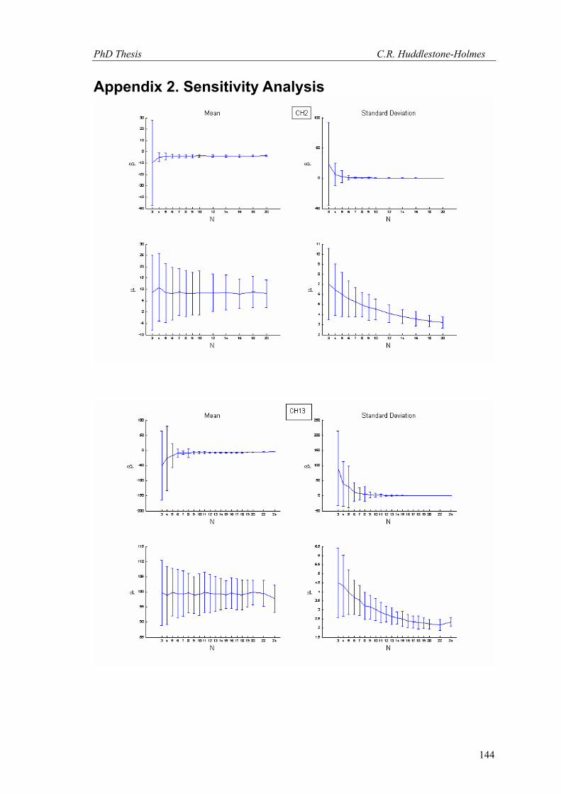
PhD Thesis C.R. Huddlestone-Holmes
144
Appendix 2. Sensitivity Analysis
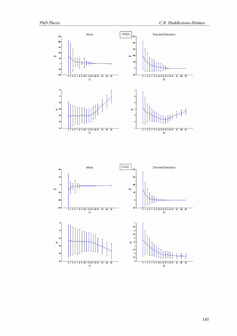
PhD Thesis C.R. Huddlestone-Holmes
145
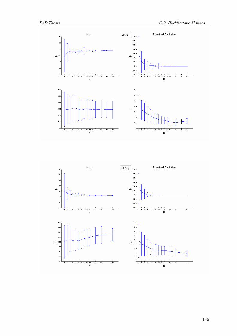
PhD Thesis C.R. Huddlestone-Holmes
146
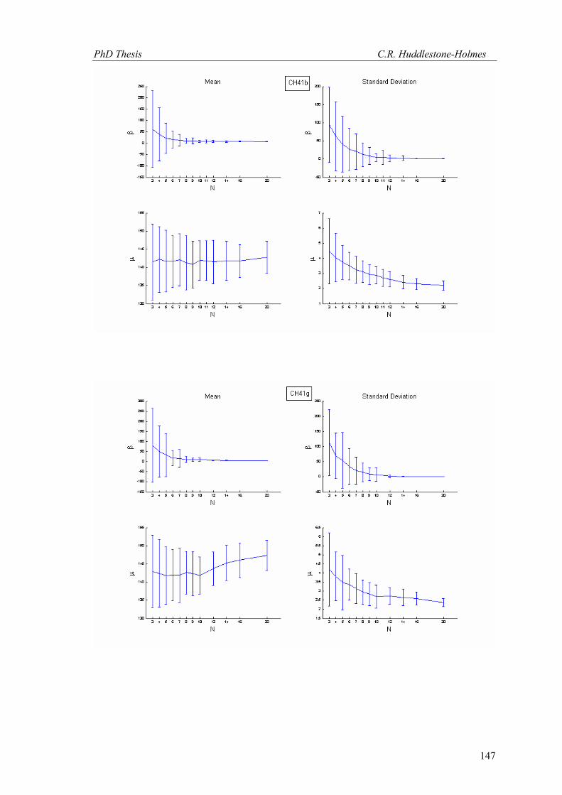
PhD Thesis C.R. Huddlestone-Holmes
147
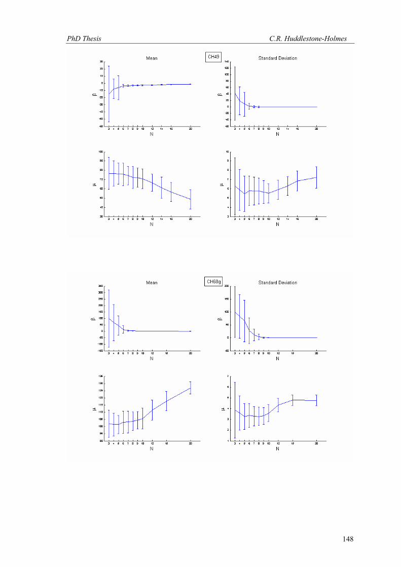
PhD Thesis C.R. Huddlestone-Holmes
148
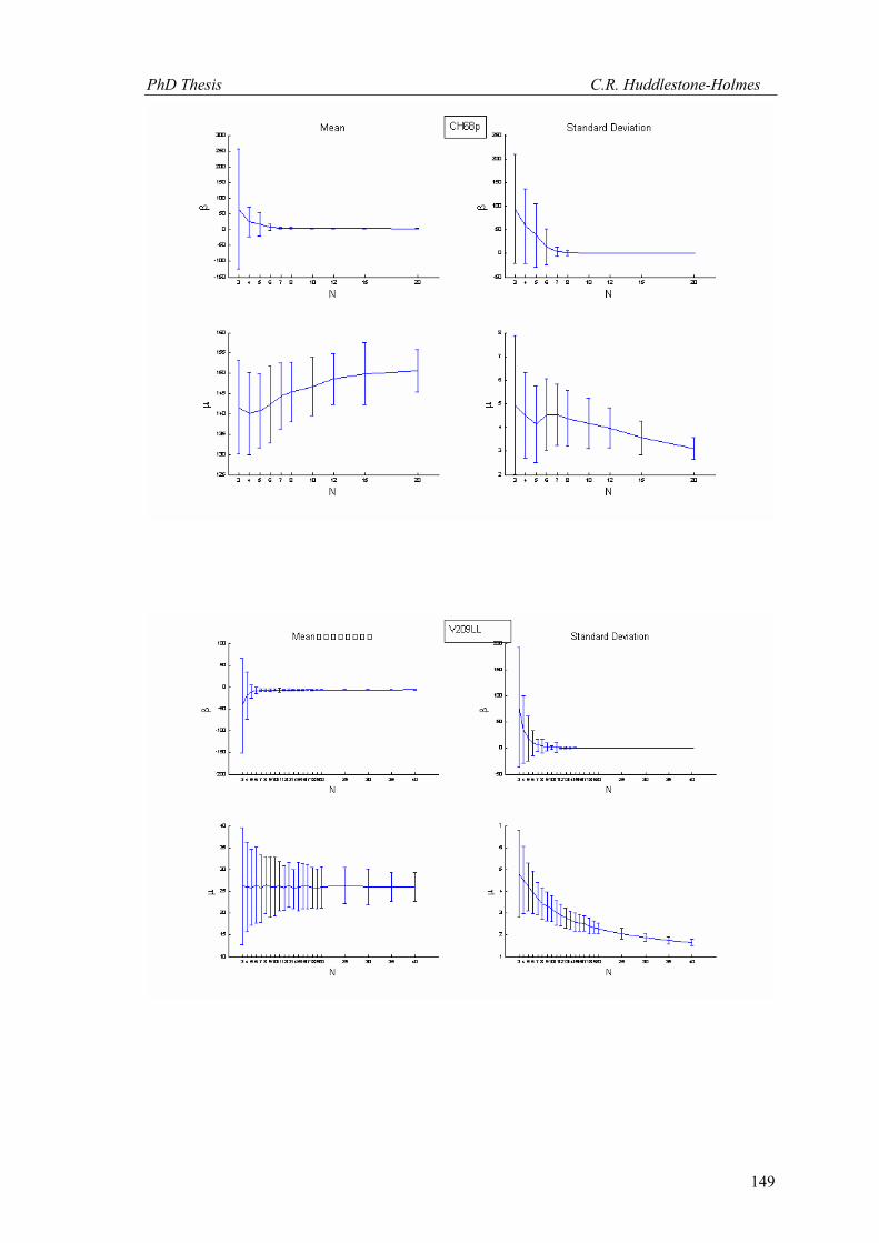
PhD Thesis C.R. Huddlestone-Holmes
149
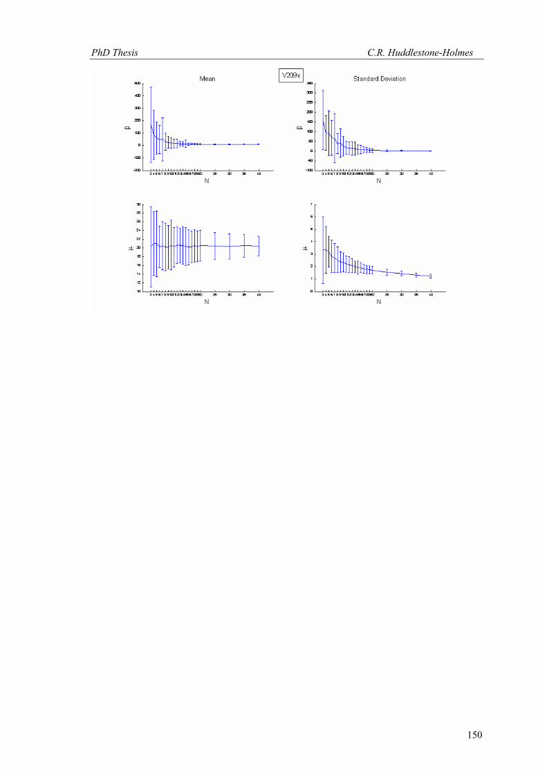
PhD Thesis C.R. Huddlestone-Holmes
150

PhD Thesis C.R. Huddlestone-Holmes
151
Conclusions
PhD Thesis C.R. Huddlestone-Holmes
152
This thesis has addressed several of the key concerns regarding FIA data, as well as
developing new techniques for studying FIAs. Chapter 1 demonstrated how HRXCT could be
used to analyse the three-dimension geometries of inclusion trails in garnet porphyroblasts.
Guidelines for sample selection for such studies are as follows. Firstly, 5 to 10 mm diameter
garnets that could be scanned individually, or in cores drilled from a sample, provide a voxel
size of 5 to 10 microns, which is the optimal resolution. Scanning a larger sample at low
resolution would allow the garnets within it to be located so that they can be extracted. Inclusion
trails composed of minerals with significantly different attenuation coefficients to garnet are
necessary to provide high contrast. Quartz and iron/titanium oxides, which are common
inclusions in garnet, are ideal. Given the voxel size described above, an inclusion size ranging
from fifty microns to 0.2 mm in maximum dimension is ideal. This size allows the shape of
individual inclusions to be clearly imaged. An appropriate range for the inclusion density is
from ten to thirty percent. If the density is too high, images are confusing; if it is too low, the
trails are not adequately defined.
The second chapter uses data generated by the HRXCT technique described in chapter 1
to determine the range of FIA orientations in single sample. A FIA was measured in the core of
58 porphyroblasts. The FIAs have a moderate to tightly clustered distribution that is difficult to
reconcile with a rotational hypothesis for the formation of curved inclusion trail, particular in
light of the subsequent deformation events that affected this sample. One of the latter events
formed a FIA in the median of the porphyroblasts that has a trend at approximately 90° to that
in the core. The most likely source of variation in FIA orientations, which formed during a
particular stage of porphyroblast growth in a single sample, is in the variation of the foliations
that form them.
The third chapter presents the background for a technique that can be used to quantify
the accuracy of FIAs measured using the asymmetry method. It also provides a measure of the
distribution of FIAs in a sample. The technique uses maximum likelihood estimation (MLE) to
fit a cyclic logistic regression to asymmetry data. By applying bootstrapping to this approach,
flaws in the assumptions regarding the goodness-of-fit test for the original technique were
highlighted. As a result, graphical procedures for determining the fit of the model to the data
were suggested, based on examining the distributions of the bootstrapped parameters and the
model deviance. The fact that the technique is sensitive to sample size was also highlighted.
As part of a demonstration of the application of the bootstrapped MLE approach
(chapter 4), an analysis of its sensitivity to the number of observations in each section
orientation was made. The results of this suggest that a minimum of 10 observations per section
orientation are needed in the vicinity of the FIA to produce repeatable results. The FIA
distributions described in chapter 4 agree with the results of chapter 2, and show that their range
in a sample will generally be in the order of 40° to 80°. These distributions are unimodal,
PhD Thesis C.R. Huddlestone-Holmes
153
symmetrical and have a peak at their mean, and the probabilities decay monotonically away
from it, as occurs in a normal distribution.
A FIA set is the term given to a group of FIA orientations from different samples that
are interpreted to have formed at the same time. The correlation of FIAs between samples
should be done based on orientation and relative timing criteria. Using inclusion trail textures
assumes that metamorphic and strain conditions were similar in the samples being compared.
This is precarious because deformation partitioning can result in highly variable distributions of
strain. Therefore, the intensity of a foliation preserved in porphyroblasts is totally unreliable for
such correlations. With large datasets, determining the error in individual FIA measurements is
not important, because the errors will tend to average out. Placing a particular FIA measurement
in one FIA set or the other that have similar orientations requires appropriate relative timing
criteria. The distribution of FIAs in a FIA set is similar to that for a FIA in a sample.
Providing estimates of the error in the measured FIA orientation are essential if FIA
orientations are used as timing markers for P-T calculations and age determinations, or for
detailed analysis of structural processes at outcrop scale,. Inferences made based on FIA data
are strengthened when this is done.
FIAs have been demonstrated to have consistent regional patterns that can be correlated
along orogens. It is difficult to conceive how such distributions can develop if rotation of
porphyroblasts relative to each other is a common phenomenon. This suggests that they do
reflect plate scale processes and that their orientations relate to the relative direction of plate
motion.
This thesis has addressed many of the questions regarding the distribution of FIAs and
their significance. It has examined their distribution in a single sample, provided a method for
determining the error in FIA measurements made using the asymmetry method, and discussed
the application and significance of FIA data in detailed and regional studies. This framework
will enhance future applications of FIA data by ensuring that their interpretations are
statistically valid.
Directions for Future Research The following are avenues for future research that follow on from the work described
herein.
The application of the HRXCT technique in this thesis was focussed on the specific
problem of the distribution of FIA in a single sample. This technique could also be applied to
detailed studies of the three-dimensional geometry of curved inclusion trails in garnet. This may
help address the ongoing controversy of the mode of formation of these features. It could also
be conducted in conjunction with electron microprobe analysis to investigate the relationships
between compositional zoning and microstructures. This would provide insight into the links
between metamorphic and microstructural processes.
PhD Thesis C.R. Huddlestone-Holmes
154
The FIA distribution was measured for a single sample in chapter 2. It would be useful
to apply this technique to a number of samples to determine if the intra sample distribution of
FIAs varies between samples. Samples with a range of inclusion trail geometries could be
studied, including those with true spirals.
The goodness-of-fit test for the cyclic logistic model described in chapter 3 uses a
graphical approach. A formal approach that can be used in conjunction with this is highly
desirable. Such a test requires the issue of dependant chi-squared distributions with fractional
degrees of freedom to be addressed. This is a problem that has received very little attention in
the literature.
A result of the growing body of FIA data are questions regarding the processes that
form foliations. The variation in FIA orientations appears to represent the variation in the
orientation of the foliations that form them. It is typically accepted that foliations form
perpendicular to the direction of bulk shortening. A difficulty with this interpretation is that
shear should not occur on surfaces that are perpendicular to the axis of principal stress. The fact
that porphyroblast rotation is highly unlikely also suggests that strain models that include
pervasive spin and vorticity are also problematic. The progressive, bulk inhomogeneous
shortening (PBIS) model addresses these issues by partitioning deformation into zones of
shortening and anastomosing zones of shearing. Clearly more work needs to be done to
investigate how foliations form in order to address the issues of lack of porphyroblast rotation,
and the relationship between stress and strain as cleavages form.