
INSTITUTE OF NATURAL AND APPLIED SCIENCES UNIVERSITY … · institute of natural and applied...
88
INSTITUTE OF NATURAL AND APPLIED SCIENCES UNIVERSITY OF CUKUROVA PhD THESIS Banu ¨ OZEL STUDY OF THE 112,120 Sn (γ, γ ′ ) REACTION AND SYSTEMATICS OF THE PYGMY DIPOLE RESONANCE AT THE Z=50 SHELL CLOSURE DEPARTMENT OF PHYSICS ADANA, 2008
Transcript of INSTITUTE OF NATURAL AND APPLIED SCIENCES UNIVERSITY … · institute of natural and applied...
INSTITUTE OF NATURAL AND APPLIED SCIENCES
UNIVERSITY OF CUKUROVA
PhD THESIS
Banu OZEL
STUDY OF THE 112,120Sn (γ,γ′) REACTION AND SYSTEMATICS OF THEPYGMY DIPOLE RESONANCE AT THE Z=50 SHELL CLOSURE
DEPARTMENT OF PHYSICS
ADANA, 2008
CUKUROVA UNIVERSITESI
FEN BIL IMLER I ENSTIT USU
112,120Sn(γ,γ′) REAKSIYONU VE Z=50 KAPALI KABUKLARINDA PYGMY
DIPOL REZONANSI S ISTEMAT IGIN IN INCELENMES I
Banu OZEL
DOKTORA TEZ I
FIZ IK ANAB IL IM DALI
Bu tez ......................... tarihinde asagıdaki juri uyeleri tarafından oybirligi/oycoklugu ilekabul edilmistir.
Imza.............................Prof.Dr. Suleyman GUNGOR1. DANISMAN
Imza.............................Prof.Dr. Peter von NEUMANN-COSEL2. DANISMAN
Imza.............................Prof.Dr. MetinOZDEMIRUYE
Imza.............................Prof.Dr. Sefa ERTURKUYE
Imza.............................Prof.Dr. GulsenONENGUTUYE
Bu tez Enstitumuz Fizik Anabilim Dalında hazırlanmıstır.Kod No:
Prof.Dr. Aziz ERTUNCEnstitu MuduruImza ve Muhur
Bu Calısma DFG-SFB634, Erasmus-Sokrates Student Exchange Program ve DAADTarafından Desteklenmistir.
Not: Bu tezde kullanılanozgun ve baska kaynaktan yapılan bildirislerin, cizelge, sekil ve fotog-rafların kaynak gosterilmeden kullanımı, 5846 sayılı Fikir ve Sanat Eserleri Kanunundaki hukum-lere tabidir.
OZ
DOKTORA TEZ I
112,120Sn(γ,γ′) REAKSIYONU VE Z=50 KAPALI KABUKLARINDA PYGMY
DIPOL REZONANSI S ISTEMAT IGIN IN INCELENMES I
Banu OZEL
CUKUROVA UNIVERSITESI
FEN BIL IMLER I ENSTIT USU
FIZ IK ANAB IL IM DALI
Danısman: Prof.Dr. Suleyman GUNGOR2. Danısman: Prof.Dr. Peter von NEUMANN-COSEL
Yıl: 2008, Sayfa: 75
Juri: Prof.Dr. Suleyman GUNGOR
Prof.Dr. Peter von NEUMANN-COSELProf.Dr. MetinOZDEMIRProf.Dr. Sefa ERTURKProf.Dr. GulsenONENGUT
Bu tezde S-DALINAC super iletken elektron lineer hızlandırıcısında gerceklestirilen112,120Sn(γ,γ′) reaksiyonları Bremsstrahlung spektrumunun farklı son nokta enerjileri icinnotron ayrısma enerjisinin altındaki bolgelerde calısılmıstır.112Sn cekirdegi icin 9.5MeV‘ye, 120Sn cekirdegi icin 7.5 ve 9.1 MeV‘ye kadar dipol gecis siddetleri dagılımıolusturulmustur. Elde edilen sonuclar hali hazırda varolan116,124Sn (Govaert, ve ark.,1998) verileri ile birlikte notron fazlalıgı olan cekirdeklerde bulunan pygmy dipol rezo-nansı olarak adlandırılan yapı hakkında bilgi edinmemizi saglamıstır. Buna ek olarakparcalanma analizi denilen bir analiz metodu foton sacılması ile elde edilmis olan spek-trumlara, parcalanmadan kaynaklanan ve fonda bulunan cozulmemis gecis siddetlerininmiktarlarını tahmin edebilmek amacıyla uygulanmıstır.
Sonuclar quasiparticle phonon modeli ve relativistik quasiparticle RPA ilekarsılastırılmıstır.
Anahtar Kelimeler: Pygmy Dipol Rezonansı, E1 gecis siddeti, nukleer rezonans fluo-resans metodu, parcalanma analizi
I
ABSTRACT
PhD THESIS
STUDY OF THE 112,120Sn (γ,γ′) REACTION AND SYSTEMATICS OF THE
PYGMY DIPOLE RESONANCE AT THE Z=50 SHELL CLOSURE
Banu OZEL
DEPARTMENT OF PHYSICS
INSTITUTE OF NATURAL AND APPLIED SCIENCES
UNIVERSITY OF CUKUROVA
Supervisor: Prof.Dr. Suleyman GUNGOR2. Supervisor: Prof.Dr. Peter von NEUMANN-COSEL
Year: 2008, Pages: 75
Jury: Prof.Dr. Suleyman GUNGOR
Prof.Dr. Peter von NEUMANN-COSELProf.Dr. MetinOZDEMIRProf.Dr. Sefa ERTURKProf.Dr. GulsenONENGUT
In this thesis the112,120Sn(γ,γ′) reactions are studied at different endpoint energies ofthe incident bremsstrahlung spectrum below the neutron separation energies at the super-conducting Darmstadt electron linear accelerator S-DALINAC. Dipole transition strengthdistributions are extracted for112Sn up to 9.5 MeV and for120Sn up to 9.1 MeV. A concen-tration of dipole excitations is observed between 5 and 8 MeV. Furthermore a fluctuationanalysis is applied to the photon scattering spectra to estimate the amount of the unre-solved strength hidden in background due to fragmentation of the strength. Together withexisting data for116,124Sn (Govaert, et al., 1998) this provides a set of information on thestructure of the so-called pygmy dipole resonance (PDR) in the stable neutron-rich tinnuclei.
The results are compared to microscopic quasiparticle-phonon model and relativisticquasiparticle RPA calculations.
Key Words: Pygmy Dipole Resonance, E1 transition strength, Nuclear Resonance Fluo-rescence, fluctuation analysis
II
ACKNOLEDGEMENTS
This work would not have been imaginable without help and support of many people
who also I have been not mentioned directly their name at this place.
I would like to express my deep and sincere gratitude to Prof. Dr. Peter von Neumann-
Cosel for the supervision of my work. His very broad knowledge, help and suggestions
were highly important for me and absolutely crucial in bringing this thesis to completion.
I would like to thank Prof. Dr. h. c. mult. Achim Richter who kindly accepted me in
his group in Institut fur Kernphysik (IKP) at Technische Universitat Darmstadt.
Further on I would like to thank my second supervisor Prof. Dr. Suleyman Gungor for
his continuous support and care during my stay in Cukurova University and in Germany.
I would like to acknowledge Prof. Dr. Sefa Erturk who introduced me to the field of
experimental nuclear physics and supported me during all stage of my scientific work.
I am also indebted to Prof. Dr. Joachim Enders, Dr. Yaroslav Kalmykov for numerous
discussion during my work.
I owe my sincere gratitude to my colleges at IKP: Dr. Stephan Volz, Dr. Deniz
Savran, Dr. Kai Lindenberg, Linda Schnorrenberger, Jens Hasper, Michael Elvers, Iryna
Poltoratska who helped me during my experiments and performing the analysis.
I am very grateful to Dr. Nadia Tsoneva, Dr. V.Yu. Ponomarev, Dr. Nils Paar for pro-
viding theoretical calculations and their fruitful suggestions in theoretical interpretation
of the experimental results.
I address my heartfelt gratitude to Dr. Harald Genz and Sabine Genz for their help,
care, support and valuable friendship. I will never forget you.
I wish to thank head of our department, Prof Dr. Yuksel Ufuktepe and Prof. Dr. Metin
Ozdemir from Cukurova University for their understanding, help and support.
I wish to express my warm thanks to Dilek KoyuncuOzen, CemOzen, Numan
Bakırcı, Ayse Seyhan, Yi ˘git Yıldız, Sarla Rathi, Barbara Sulignano, Haris Djapo. I am
very happy to meet with you.
Finally I would like to thank to my parents and my brother Tayfun for support, under-
standing and being always together with me. Particularly I would like to express my most
important thanks to my fiance, Dr. Stanislav Tashenov for his love, encouragement and
patience during my work.
III
TABLE OF CONTENTS PAGE
OZ . . . . . . . . . . . . . . . . . . . . . . . . . . . . . . . . . . . . . . . . . . I
ABSTRACT . . . . . . . . . . . . . . . . . . . . . . . . . . . . . . . . . . . . . II
ACKNOLEDGEMENTS . . . . . . . . . . . . . . . . . . . . . . . . . . . . . . . III
TABLE OF CONTENTS . . . . . . . . . . . . . . . . . . . . . . . . . . . . . . . IV
LIST OF TABLES . . . . . . . . . . . . . . . . . . . . . . . . . . . . . . . . . . VI
LIST OF FIGURES . . . . . . . . . . . . . . . . . . . . . . . . . . . . . . . . . VII
LIST OF SYMBOLS AND ABBREVIATIONS . . . . . . . . . . . . . . . . . . . IX
1 INTRODUCTION . . . . . . . . . . . . . . . . . . . . . . . . . . . . . . . . 1
2 PREVIOUS WORKS . . . . . . . . . . . . . . . . . . . . . . . . . . . . . . . 3
3 MATERIAL and METHOD . . . . . . . . . . . . . . . . . . . . . . . . . . . 5
3.1 Collective Excitations in Nuclei . . . . . . . . . . . . . . . . . . . . . . 5
3.1.1 Giant Resonances . . . . . . . . . . . . . . . . . . . . . . . . . . 5
3.1.1.1 Classification of Giant Resonances . . . . . . . . . . . 5
3.1.2 Electric Dipole Excitations in Nuclei . . . . . . . . . . . . . . . 8
3.1.2.1 Giant Dipole Resonance . . . . . . . . . . . . . . . . . 9
3.1.2.2 Pygmy Dipole Resonance . . . . . . . . . . . . . . . . 10
3.2 Nuclear Resonance Fluorescence (NRF) Method . . . . . . . . . . . . . 13
3.2.1 Integrated Cross Section . . . . . . . . . . . . . . . . . . . . . . 15
3.2.2 Transition Width and Transition Strength . . . . . . . . . . . . . 17
3.2.3 Angular Distribution . . . . . . . . . . . . . . . . . . . . . . . . 18
3.3 Photon Scattering Experiments at the S-DALINAC . . . . . . . . . . . . 21
3.3.1 The S-DALINAC . . . . . . . . . . . . . . . . . . . . . . . . . . 21
3.3.2 NRF Setup . . . . . . . . . . . . . . . . . . . . . . . . . . . . . 23
3.3.3 Detectors . . . . . . . . . . . . . . . . . . . . . . . . . . . . . . 24
IV
3.3.4 BGO Suppression . . . . . . . . . . . . . . . . . . . . . . . . . 27
4 ANALYSIS and RESULTS . . . . . . . . . . . . . . . . . . . . . . . . . . . . 30
4.1 Analysis of Resolved Transitions . . . . . . . . . . . . . . . . . . . . . . 30
4.1.1 Experimental Details . . . . . . . . . . . . . . . . . . . . . . . . 30
4.1.2 Detector Efficiency . . . . . . . . . . . . . . . . . . . . . . . . . 33
4.1.3 Spin Determination . . . . . . . . . . . . . . . . . . . . . . . . . 33
4.1.4 Photon Flux and Integrated Cross Section . . . . . . . . . . . . . 35
4.1.5 Estimation of the Feeding Effect . . . . . . . . . . . . . . . . . . 38
4.1.6 Reduced Transition Strengths . . . . . . . . . . . . . . . . . . . 40
4.1.7 Systematics of the E1 Strength in Stable Tin Isotopes . . . . . . . 46
4.2 Fluctuation Analysis . . . . . . . . . . . . . . . . . . . . . . . . . . . . 48
4.2.1 Theoretical Models . . . . . . . . . . . . . . . . . . . . . . . . . 48
4.2.1.1 Back-Shifted Fermi Gas Model . . . . . . . . . . . . . 49
4.2.1.2 Hartree-Fock-BCS Model . . . . . . . . . . . . . . . . 51
4.2.2 Fluctuation Analysis Method . . . . . . . . . . . . . . . . . . . . 52
4.2.3 Application to Photon Scattering Spectra . . . . . . . . . . . . . 56
5 DISCUSSION and CONCLUSION . . . . . . . . . . . . . . . . . . . . . . . 63
5.1 Comparison with Theoretical Models . . . . . . . . . . . . . . . . . . . 63
5.1.1 Quasiparticle Phonon Model (QPM) . . . . . . . . . . . . . . . . 63
5.1.2 Relativistic Quasiparticle Random Phase Approximation (R QRPA) 66
5.1.3 Discussion . . . . . . . . . . . . . . . . . . . . . . . . . . . . . 67
5.2 Conclusion and Outlook . . . . . . . . . . . . . . . . . . . . . . . . . . 69
REFERENCES . . . . . . . . . . . . . . . . . . . . . . . . . . . . . . . . . . . . 71
CURRICULUM VITAE . . . . . . . . . . . . . . . . . . . . . . . . . . . . . . . 75
V
LIST OF TABLES PAGE
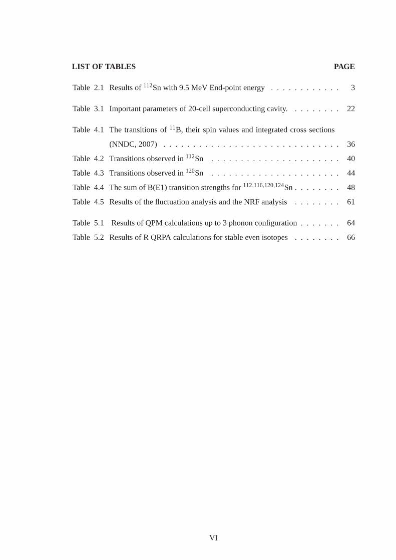
Table 2.1 Results of112Sn with 9.5 MeV End-point energy . . . . . . . . . . . . 3
Table 3.1 Important parameters of 20-cell superconducting cavity. . . . . . . . . 22
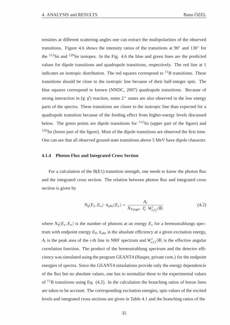
Table 4.1 The transitions of11B, their spin values and integrated cross sections
(NNDC, 2007) . . . . . . . . . . . . . . . . . . . . . . . . . . . . . . 36
Table 4.2 Transitions observed in112Sn . . . . . . . . . . . . . . . . . . . . . . 40
Table 4.3 Transitions observed in120Sn . . . . . . . . . . . . . . . . . . . . . . 44
Table 4.4 The sum of B(E1) transition strengths for112,116,120,124Sn . . . . . . . . 48
Table 4.5 Results of the fluctuation analysis and the NRF analysis . . . . . . . . 61
Table 5.1 Results of QPM calculations up to 3 phonon configuration . . . . . . . 64
Table 5.2 Results of R QRPA calculations for stable even isotopes . . . . . . . . 66
VI
LIST OF FIGURES PAGE
Figure 1.1 Measured even-even isotopes in the tin isotopic chain . . . . . . . . . 2
Figure 3.1 Classification of giant resonances based on a macroscopic picture . . . 6
Figure 3.2 Schematic picture of E1 and E2(E0) single-particle transition . . . . . 7
Figure 3.3 Electric dipole excitations in nuclei . . . . . . . . . . . . . . . . . . . 8
Figure 3.4 Possible configurations in macroscopic picture of PDR . . . . . . . . . 11
Figure 3.5 The simplified picture of NRF process . . . . . . . . . . . . . . . . . 14
Figure 3.6 The excitation-deexcitation scheme in NRF experiments . . . . . . . . 15
Figure 3.7 Angular distribution patterns for dipole and quadrupole cascades . . . 20
Figure 3.8 Schematic layout of the S-DALINAC . . . . . . . . . . . . . . . . . . 21
Figure 3.9 20-cell 3 GHz superconducting cavity. . . . . . . . . . . . . . . . . . 22
Figure 3.10Experimental facilities at the S-DALINAC. . . . . . . . . . . . . . . . 23
Figure 3.11Schematic layout of the NRF setup at the S-DALINAC . . . . . . . . . 24
Figure 3.12Scheme of a n-type coaxial HPGe detector . . . . . . . . . . . . . . . 25
Figure 3.13Principle of SE and DE . . . . . . . . . . . . . . . . . . . . . . . . . 27
Figure 3.14Typical construction of HPGe detector with BGO shield . . . . . . . . 28
Figure 3.15Spectra of the112Sn(γ,γ′) spectra atE0=9.5 with BGO and without BGO 28
Figure 4.1 Measured spectra for112Sn up to 9.5 MeV at 90◦ and 130◦ . . . . . . 30
Figure 4.2 One example of a tin target together with two11B targets) . . . . . . . 31
Figure 4.3 Measured spectra for120Sn up to 7.5 MeV at 90◦ and 130◦ . . . . . . 32
Figure 4.4 Measured spectra for120Sn up to 9.1 MeV at 90◦ and 130◦ . . . . . . 32
Figure 4.5 Absolute efficiency at 90◦ and at 130◦ for 112Sn . . . . . . . . . . . . 33
Figure 4.6 Intensity ratio of transitions in112Sn and120Sn . . . . . . . . . . . . . 34
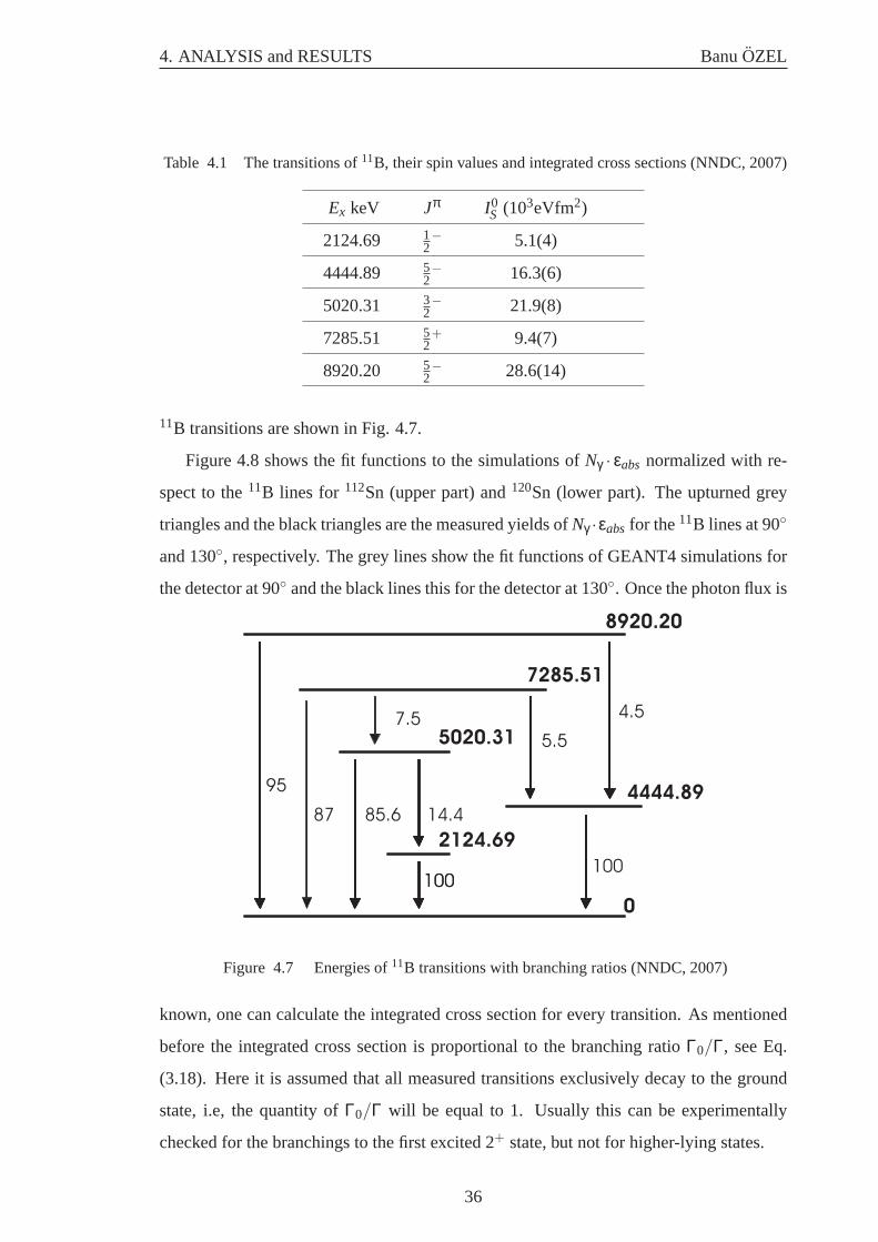
Figure 4.7 Energies of11B transitions with branching ratios . . . . . . . . . . . . 36
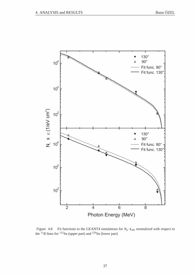
Figure 4.8 The simulation of photon flux at 130◦ for 112Sn and120Sn . . . . . . . 37
Figure 4.9 Ratio of the B(E1) transition strengths for112Sn . . . . . . . . . . . . 39
Figure 4.10Ratio of the B(E1) transition strengths for120Sn . . . . . . . . . . . . 39
Figure 4.11Comparison of the B(E1) strength in112,116,120,124Sn . . . . . . . . . 47
Figure 4.12The steps of the fluctuation analysis . . . . . . . . . . . . . . . . . . . 54
Figure 4.13Calculated level spacing,<D> for 112Sn from models . . . . . . . . . 57
VII
Figure 4.14Calculated level spacing,<D> for 120Sn from models . . . . . . . . . 57
Figure 4.15112Sn spectrum at 90◦ and calculated backgrounds . . . . . . . . . . . 59
Figure 4.16112Sn spectrum at 130◦ and calculated backgrounds . . . . . . . . . . 59
Figure 4.17120Sn spectrum at 90◦ and calculated backgrounds . . . . . . . . . . . 60
Figure 4.18120Sn spectrum at 130◦ and calculated backgrounds . . . . . . . . . . 60
Figure 4.19GEANT4 simulation of the ratio of SE to photopeak . . . . . . . . . . 61
Figure 5.1 Results of QPM calculations up to 3 phonon configuration for120Sn . . 64
Figure 5.2 The comparison with QPM:E1 strength distribution of112Sn . . . . . . 65
Figure 5.3 The comparison with QPM:E1 strength distribution of120Sn . . . . . . 65
Figure 5.4 Comparison with theory:∑B(E1) strengths and centroid energies . . . 68
VIII
LIST OF SYMBOLS AND ABBREVIATIONS
A Mass number
Z Proton number
N Neutron number
J Spin
γ Gamma radiation
β Beta radiation
GDR Giant Dipole Resonance
PDR Pygmy Dipole Resonance
GMR Giant Monopole Resonance
GQR Giant Quadrupole Resonance
S−DALINAC Superconducting Darmstadt electron linear accelerator
QCLAM Quadrupole-clamshell magnetic spectrometer
GSI Geselschaft fur Schwerionenforschung mbH
NRF Nuclear Resonance Fluorescence
GEANT4 Simulation program
E1 Electric dipole transition
EWSR Energy-weighted sum rule
TRK Thomas-Reiche-Kuhn
RPA Random phase approximation
QRPA Quasiparticle random phase approximation
QPM Quasiparticle phonon model
DFT Density fluctuation theory
DD−ME Density dependent meson exchange
ETFFS Extended theory of finite fermion systems
HPGe High purity germanium detector
BGO Bi4Ge3O2
ESS Escape suppresed spectrometer
SE Single escape
DE Double escape
λ multipolarity
IX

B(E1) Reduced transition probability of an electric dipole transition
B(M1) Reduced transition probability of a magnetic dipole transition
B(E2) Reduced transition probability of an electric quadrupole transition
Γ Width
Ex Excitation energy
Eγ Photon energy
σ Cross section
I Integrated cross section
g statistical g factor
Nγ Photon flux
εabs Absolute efficiency
M Mass of nucleus
ν Velocity of nuclei
θ Theta, angle
∆ Doppler width
e Electron charge
~ Planck constant/2π
π Pi number
µA Microampere
c Speed of light
k Boltzmann constant
f m Femtometer
meV Millielectronvolt
keV Kiloelectronvolt
MeV Megaelectronvolt
K Kelvin
T Temperature
Pλ(Θ) Legendre polynomial function
W(θ) Angular correlation function
X

NLD Nuclear level density
σ Spin cut-off parameter
a Level density parameter
MLD Microscopic liquid-drop mass
BSFG Back shifted fermi gas model
HF −BCS Hartree Fock BCS model
< D > Mean level spacing
< Γ > Mean level width
β One of BSFG free parameters
γ One of BSFG free parameters
α One of BSFG free parameters
∆E Energy resolution
C(ε) Autocorrelation function
ε shift parameter
XI
1. INTRODUCTION BanuOZEL
1. INTRODUCTION
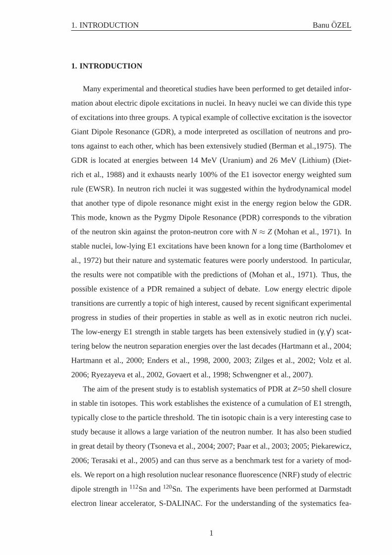
Many experimental and theoretical studies have been performed to get detailed infor-
mation about electric dipole excitations in nuclei. In heavy nuclei we can divide this type
of excitations into three groups. A typical example of collective excitation is the isovector
Giant Dipole Resonance (GDR), a mode interpreted as oscillation of neutrons and pro-
tons against to each other, which has been extensively studied (Berman et al.,1975). The
GDR is located at energies between 14 MeV (Uranium) and 26 MeV (Lithium) (Diet-
rich et al., 1988) and it exhausts nearly 100% of the E1 isovector energy weighted sum
rule (EWSR). In neutron rich nuclei it was suggested within the hydrodynamical model
that another type of dipole resonance might exist in the energy region below the GDR.
This mode, known as the Pygmy Dipole Resonance (PDR) corresponds to the vibration
of the neutron skin against the proton-neutron core withN ≈ Z (Mohan et al., 1971). In
stable nuclei, low-lying E1 excitations have been known for a long time (Bartholomev et
al., 1972) but their nature and systematic features were poorly understood. In particular,
the results were not compatible with the predictions of (Mohan et al., 1971). Thus, the
possible existence of a PDR remained a subject of debate. Low energy electric dipole
transitions are currently a topic of high interest, caused by recent significant experimental
progress in studies of their properties in stable as well as in exotic neutron rich nuclei.
The low-energy E1 strength in stable targets has been extensively studied in (γ,γ′) scat-
tering below the neutron separation energies over the last decades (Hartmann et al., 2004;
Hartmann et al., 2000; Enders et al., 1998, 2000, 2003; Zilges et al., 2002; Volz et al.
2006; Ryezayeva et al., 2002, Govaert et al., 1998; Schwengner et al., 2007).
The aim of the present study is to establish systematics of PDR atZ=50 shell closure
in stable tin isotopes. This work establishes the existence of a cumulation of E1 strength,
typically close to the particle threshold. The tin isotopic chain is a very interesting case to
study because it allows a large variation of the neutron number. It has also been studied
in great detail by theory (Tsoneva et al., 2004; 2007; Paar et al., 2003; 2005; Piekarewicz,
2006; Terasaki et al., 2005) and can thus serve as a benchmark test for a variety of mod-
els. We report on a high resolution nuclear resonance fluorescence (NRF) study of electric
dipole strength in112Sn and120Sn. The experiments have been performed at Darmstadt
electron linear accelerator, S-DALINAC. For the understanding of the systematics fea-
1
1. INTRODUCTION BanuOZEL
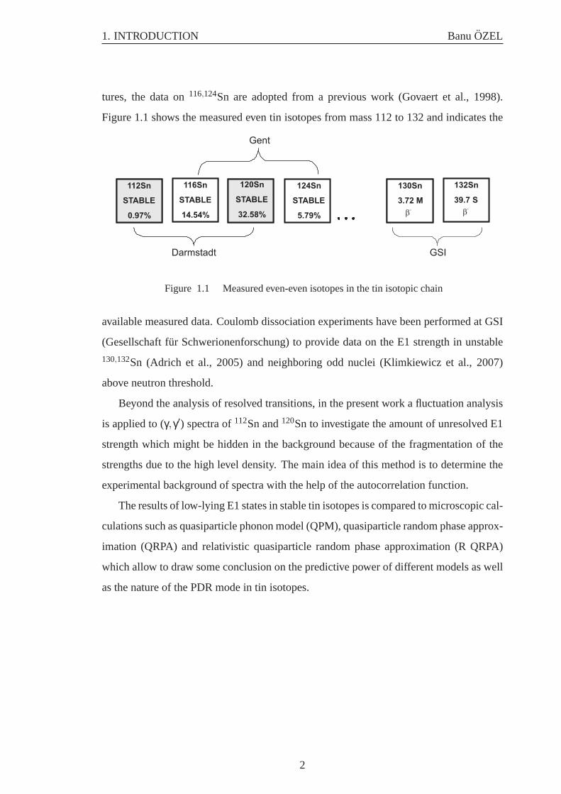
tures, the data on116,124Sn are adopted from a previous work (Govaert et al., 1998).
Figure 1.1 shows the measured even tin isotopes from mass 112 to 132 and indicates the
112SnSTABLE
0.97%
120Sn
STABLE
32.58%
116Sn
STABLE
14.54%
124Sn
STABLE
5.79%
112Sn
STABLE
0.97%
120Sn
STABLE
32.58%
116Sn
STABLE
14.54%
124Sn
STABLE
5.79%
Darmstadt
Gent
112SnSTABLE
0.97%
116Sn
STABLE
14.54%
130Sn
3.72 M
b-
132Sn
39.7 S
b-
GSI
Figure 1.1 Measured even-even isotopes in the tin isotopic chain
available measured data. Coulomb dissociation experiments have been performed at GSI
(Gesellschaft fur Schwerionenforschung) to provide data on the E1 strength in unstable
130,132Sn (Adrich et al., 2005) and neighboring odd nuclei (Klimkiewicz et al., 2007)
above neutron threshold.
Beyond the analysis of resolved transitions, in the present work a fluctuation analysis
is applied to (γ,γ′) spectra of112Sn and120Sn to investigate the amount of unresolved E1
strength which might be hidden in the background because of the fragmentation of the
strengths due to the high level density. The main idea of this method is to determine the
experimental background of spectra with the help of the autocorrelation function.
The results of low-lying E1 states in stable tin isotopes is compared to microscopic cal-
culations such as quasiparticle phonon model (QPM), quasiparticle random phase approx-
imation (QRPA) and relativistic quasiparticle random phase approximation (R QRPA)
which allow to draw some conclusion on the predictive power of different models as well
as the nature of the PDR mode in tin isotopes.
2
2. PREVIOUS WORKS BanuOZEL
2. PREVIOUS WORKS
The study of the photoresponse with (γ,γ′) experiments has been extended in recent
years to many other nuclei beyond theZ=50 region. In particular, the PDR has been
observed in44,48Ca (Hartmann et al., 2004; Hartmann et al., 2000),52Cr (Enders et al.,
1998),56Fe and58Ni (Bauwens et al., 2000),88Sr (Schwengner et al., 2007; Kubler et al.,
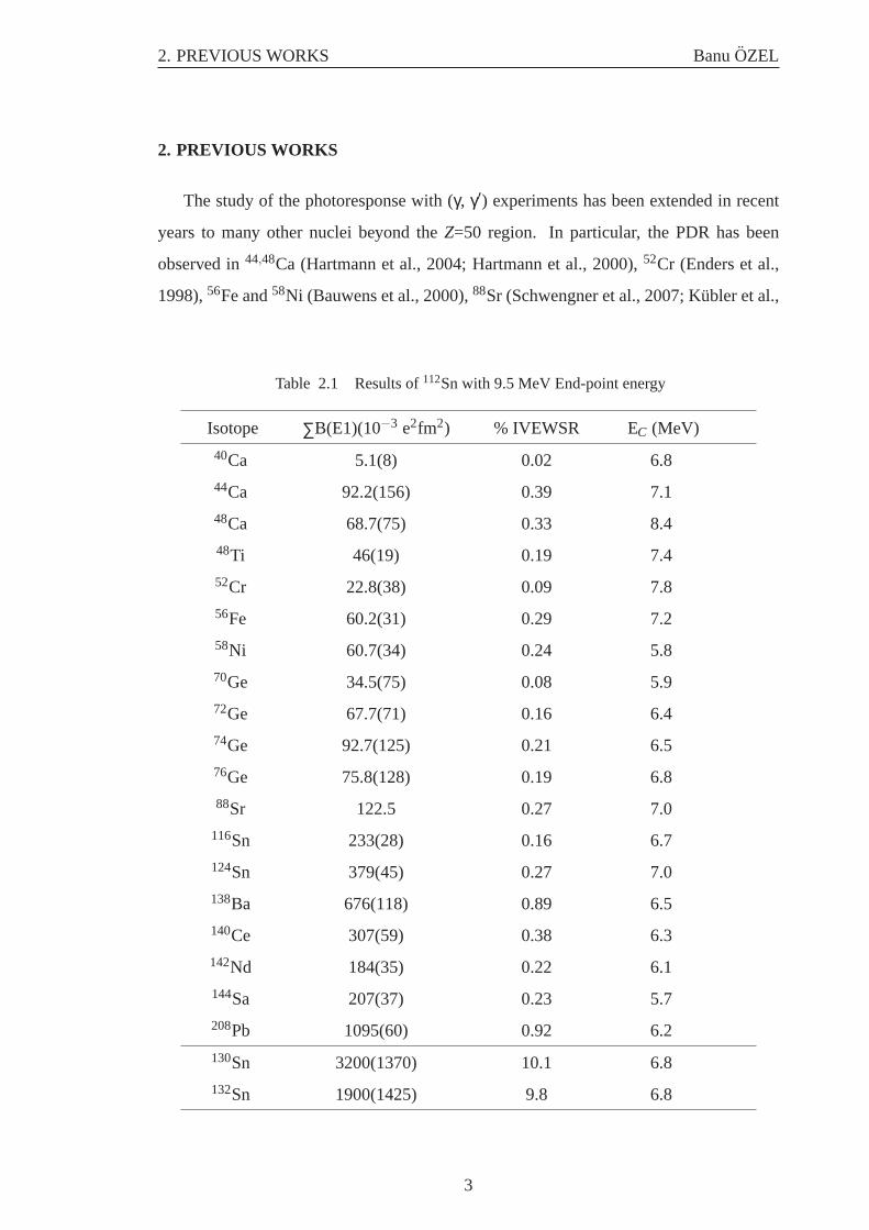
Table 2.1 Results of112Sn with 9.5 MeV End-point energy
Isotope ∑B(E1)(10−3 e2fm2) % IVEWSR EC (MeV)
40Ca 5.1(8) 0.02 6.8
44Ca 92.2(156) 0.39 7.1
48Ca 68.7(75) 0.33 8.4
48Ti 46(19) 0.19 7.4
52Cr 22.8(38) 0.09 7.8
56Fe 60.2(31) 0.29 7.2
58Ni 60.7(34) 0.24 5.8
70Ge 34.5(75) 0.08 5.9
72Ge 67.7(71) 0.16 6.4
74Ge 92.7(125) 0.21 6.5
76Ge 75.8(128) 0.19 6.8
88Sr 122.5 0.27 7.0
116Sn 233(28) 0.16 6.7
124Sn 379(45) 0.27 7.0
138Ba 676(118) 0.89 6.5
140Ce 307(59) 0.38 6.3
142Nd 184(35) 0.22 6.1
144Sa 207(37) 0.23 5.7
208Pb 1095(60) 0.92 6.2
130Sn 3200(1370) 10.1 6.8
132Sn 1900(1425) 9.8 6.8
3
2. PREVIOUS WORKS BanuOZEL
2004; Wienhard et al., 1981; Isoyama et al., 1980),92,98,100Mo (Schwengner et al., 2007),
116,124Sn (Govaert et al., 1998),N=82 isotones (Herzberg et al., 1997; Herzberg et al.,
1999; Zilges et al., 2002; Volz et al. 2006) and204,206,207,208Pb (Ryezayeva et al., 2002;
Chapuran et al., 1980; Enders et al., 2000; Enders et al., 2003). In all cases, a concentra-
tion of electric dipole strength exhausting up to 1 % of the EWSR was observed below
the neutron threshold. These results are summarized in Table 2.1. The NRF method is
restricted to stable nuclei and excitation energies roughly up to neutron separation energy.
In addition, the advent of beams of radioactive exotic nuclei allows the study of Coulomb
dissociation of neutron-rich nuclei in inverse kinematics (Aumann, 2006) for example at
the LAND setup at GSI. This method has been used already to measure dipole strength
in the exotic semi-magic130Sn, the double magic132Sn (Adrich et al., 2005) and their
neighboring odd-mass isotopes (Klimkiewicz et al., 2007). The extraction of E1 strength
was possible only above the neutron separation energies. The results for130,132Sn, which
are listed in the lower part of Table 2.1, are 5-8 times higher than the results for the most
neutron-rich stable124Sn isotope.
4
3. MATERIAL and METHOD BanuOZEL
3. MATERIAL and METHOD
3.1 Collective Excitations in Nuclei
3.1.1 Giant Resonances
Giant resonance is a term generally used to describe collective vibrations of nuclei,
which shows up as broad resonances at energies tens of MeV above the ground state.
The reason that these excitations are called ”giant” resonances comes from the fact that
both their total strength and their widths are much larger than typical resonances built on
single-particle (non-collective) excitations (Wong, 1990).
3.1.1.1 Classification of Giant Resonances
Giant resonances correspond to a collective motion involving many particles in the
nucleus. The occurrence of such a collective motion is a common feature of many-body
quantum systems. The term ”collective” here means that the majority of the nucleons
participate in the excitation. In quantum mechanical terms the resonance corresponds to
a transition between ground state and a collective state and the strength of the transition
will depend on the basic properties of the response and the size of the system. This
implies that the total transition strength should be limited by a sum rule which depends
only on ground state properties (Bohr and Mottelson, 1975). If the transition strength of
an observed resonance exhausts a major part, say greater than 50% of the corresponding
sum rule we call it a giant resonance. Within the liquid-drop model giant resonances ban
be classified according to their angular momentum,L, isospin,T, and spin,S, as illustrated
in Fig. 3.1.
• The Giant Monopole Resonance (GMR),L = 0, the so-called breathing mode.
• The Giant Dipole Resonance (GDR),L = 1 is a density/shape oscillation for the
isovector case
• The Giant Quadrupole Resonance (GQR) is a surface oscillation with angular mo-
mentumL = 2.
5
3. MATERIAL and METHOD BanuOZEL
p, n n
n
n
p
p
p n
p np n
p n
p n
p n
p
n
p
n
p
n
p
n
p
np
np, n
p
p, n
monopole
dipole
quadrupole
T = 0
S = 0
T = 1
S = 0
T = 0
S = 1
T = 1
S = 1
p, n n
n
n
p
p
p n
p np np np n
p np n
p np n
p np n
p
n
p
n
p
n
p
n
p
n
p
np
n
p
np, n
p
p, n
monopole
dipole
quadrupole
T = 0
S = 0
T = 1
S = 0
T = 0
S = 1
T = 1
S = 1
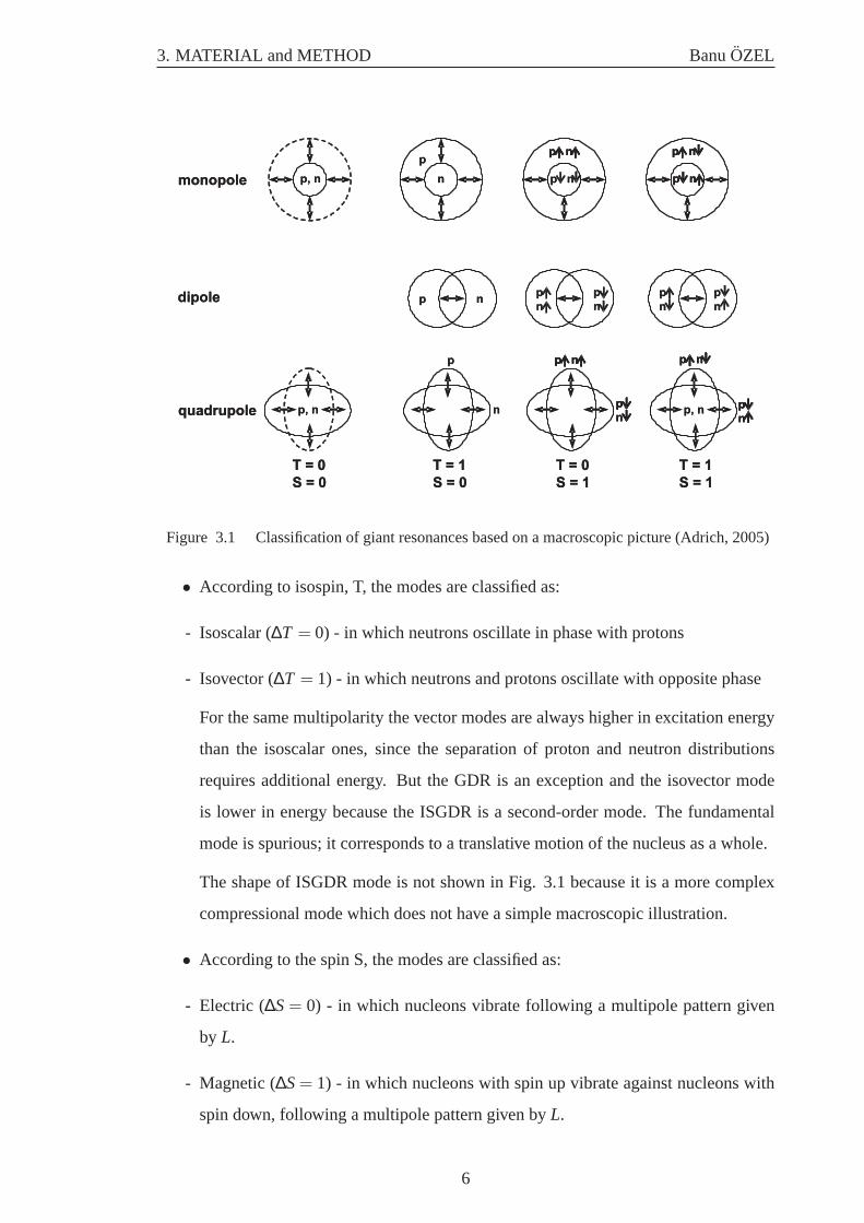
Figure 3.1 Classification of giant resonances based on a macroscopic picture (Adrich, 2005)
• According to isospin, T, the modes are classified as:
- Isoscalar (∆T= 0) - in which neutrons oscillate in phase with protons
- Isovector (∆T= 1) - in which neutrons and protons oscillate with opposite phase
For the same multipolarity the vector modes are always higher in excitation energy
than the isoscalar ones, since the separation of proton and neutron distributions
requires additional energy. But the GDR is an exception and the isovector mode
is lower in energy because the ISGDR is a second-order mode. The fundamental
mode is spurious; it corresponds to a translative motion of the nucleus as a whole.
The shape of ISGDR mode is not shown in Fig. 3.1 because it is a more complex
compressional mode which does not have a simple macroscopic illustration.
• According to the spin S, the modes are classified as:
- Electric (∆S= 0) - in which nucleons vibrate following a multipole pattern given
by L.
- Magnetic (∆S= 1) - in which nucleons with spin up vibrate against nucleons with
spin down, following a multipole pattern given byL.
6
3. MATERIAL and METHOD BanuOZEL
DN=1 DN=0 DN=2
~1hw
~1hw
E1 E2(E0)
N+1
N
N+2
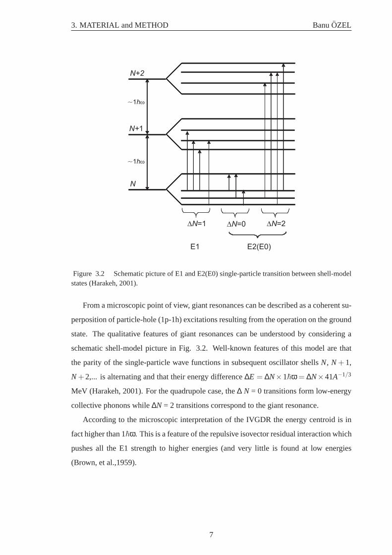
Figure 3.2 Schematic picture of E1 and E2(E0) single-particle transition between shell-modelstates (Harakeh, 2001).
From a microscopic point of view, giant resonances can be described as a coherent su-
perposition of particle-hole (1p-1h) excitations resulting from the operation on the ground
state. The qualitative features of giant resonances can be understood by considering a
schematic shell-model picture in Fig. 3.2. Well-known features of this model are that
the parity of the single-particle wave functions in subsequent oscillator shellsN, N + 1,
N+2,... is alternating and that their energy difference∆E = ∆N×1~ω = ∆N×41A−1/3
MeV (Harakeh, 2001). For the quadrupole case, the∆ N = 0 transitions form low-energy
collective phonons while∆N = 2 transitions correspond to the giant resonance.
According to the microscopic interpretation of the IVGDR the energy centroid is in
fact higher than 1~ω. This is a feature of the repulsive isovector residual interaction which
pushes all the E1 strength to higher energies (and very little is found at low energies
(Brown, et al.,1959).
7
3. MATERIAL and METHOD BanuOZEL
3.1.2 Electric Dipole Excitations in Nuclei
Throughout the last decade numerous experiments using electromagnetic probes have
provided a vast amount of data on low-lying electric dipole excitations in heavy nuclei.
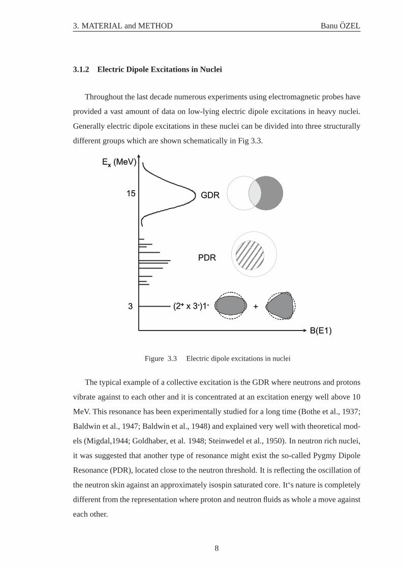
Generally electric dipole excitations in these nuclei can be divided into three structurally
different groups which are shown schematically in Fig 3.3.
3
15
PDR
GDR
(2+ x 3-)1- +
Ex (MeV)
B(E1)
3
15
PDR
GDR
(2+ x 3-)1- +
Ex (MeV)
B(E1)
Figure 3.3 Electric dipole excitations in nuclei
The typical example of a collective excitation is the GDR where neutrons and protons
vibrate against to each other and it is concentrated at an excitation energy well above 10
MeV. This resonance has been experimentally studied for a long time (Bothe et al., 1937;
Baldwin et al., 1947; Baldwin et al., 1948) and explained very well with theoretical mod-
els (Migdal,1944; Goldhaber, et al. 1948; Steinwedel et al., 1950). In neutron rich nuclei,
it was suggested that another type of resonance might exist the so-called Pygmy Dipole
Resonance (PDR), located close to the neutron threshold. It is reflecting the oscillation of
the neutron skin against an approximately isospin saturated core. It‘s nature is completely
different from the representation where proton and neutron fluids as whole a move against
each other.
8
3. MATERIAL and METHOD BanuOZEL
In addition one can observe a single strong transition at low energies in spherical
nuclei close to the magic proton or neutron shells. This is a two-phonon state which
originates from the coupling of quadrupole and octupole phonons. A coupling of these
two single phonon excitations leads to a two-phonon quintuplet (Lipas, 1966; Vogel et al.,
1971; Grinberg et al., 1994) with spinsJπ = 1−, ...,5−. A schematic representation of the
shape vibration and their assumed coupling is displayed in the lower part of the Fig. 3.3.
3.1.2.1 Giant Dipole Resonance
The GDR has been studied most extensively among all the giant resonances because
the mode is relatively easy to excite. In photonuclear reactions, i.e., in reactions in which a
nucleus is bombarded with energetic gamma rays, total cross sections for GDR excitation
are of the order of hundreds of millibarns.
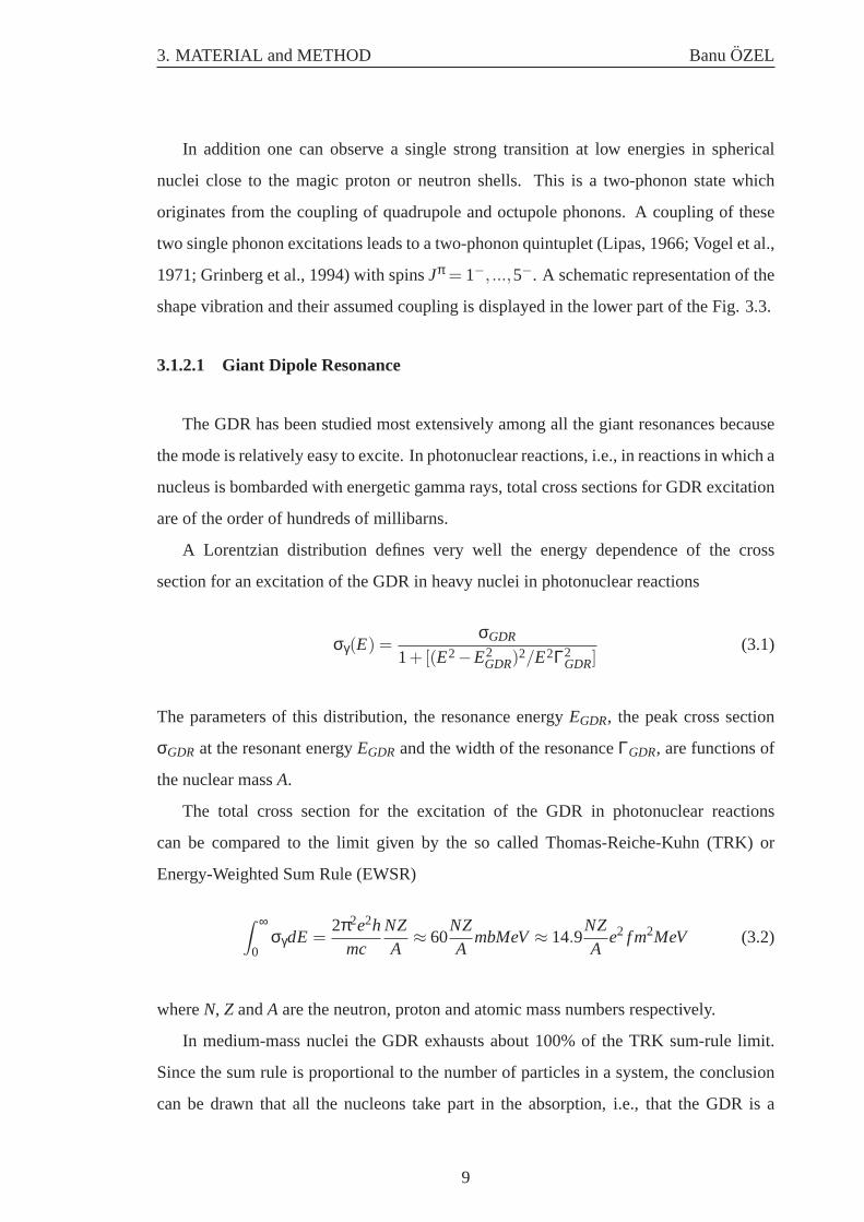
A Lorentzian distribution defines very well the energy dependence of the cross
section for an excitation of the GDR in heavy nuclei in photonuclear reactions
σγ(E) =σGDR
1+[(E2−E2GDR)
2/E2Γ2GDR]
(3.1)
The parameters of this distribution, the resonance energyEGDR, the peak cross section
σGDR at the resonant energyEGDR and the width of the resonanceΓGDR, are functions of
the nuclear massA.
The total cross section for the excitation of the GDR in photonuclear reactions
can be compared to the limit given by the so called Thomas-Reiche-Kuhn (TRK) or
Energy-Weighted Sum Rule (EWSR)
∫ ∞
0σγdE =
2π2e2hmc
NZA
≈ 60NZA
mbMeV≈ 14.9NZA
e2 f m2MeV (3.2)
whereN, Z andA are the neutron, proton and atomic mass numbers respectively.
In medium-mass nuclei the GDR exhausts about 100% of the TRK sum-rule limit.
Since the sum rule is proportional to the number of particles in a system, the conclusion
can be drawn that all the nucleons take part in the absorption, i.e., that the GDR is a
9
3. MATERIAL and METHOD BanuOZEL
collective vibration of the whole nucleus.
For heavy nuclei integrals of the experimental photonuclear section exceed the value
of the TRK sum rule, which results from exchange and velocity-dependent parts of the
nuclear potential omitted in the derivation of the TRK sum rule. In the literature those
contributions are usually included via a factorκ, introduced in the following way:
∫ ∞
0σγdE = (1+κ)60
NZA
mbMeV (3.3)
For A ≥ 90 nuclei the experimental value of(1+κ) varies from about 1 forA ≈ 100 to
1.3± 0.2 for heavy nuclei such as actinide with an average value of 1.2± 0.1 (Harakeh,
2001; Adrich, 2005).
3.1.2.2 Pygmy Dipole Resonance
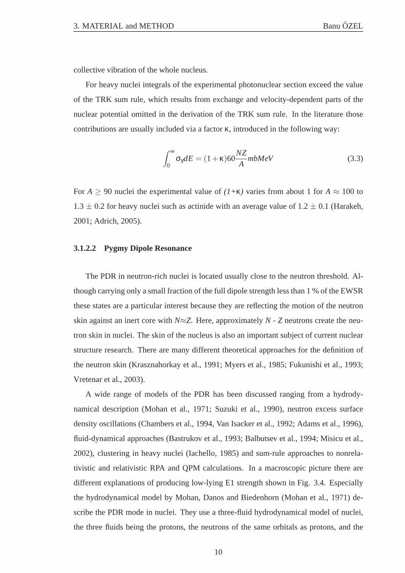
The PDR in neutron-rich nuclei is located usually close to the neutron threshold. Al-
though carrying only a small fraction of the full dipole strength less than 1 % of the EWSR
these states are a particular interest because they are reflecting the motion of the neutron
skin against an inert core withN≈Z. Here, approximatelyN - Z neutrons create the neu-
tron skin in nuclei. The skin of the nucleus is also an important subject of current nuclear
structure research. There are many different theoretical approaches for the definition of
the neutron skin (Krasznahorkay et al., 1991; Myers et al., 1985; Fukunishi et al., 1993;
Vretenar et al., 2003).
A wide range of models of the PDR has been discussed ranging from a hydrody-
namical description (Mohan et al., 1971; Suzuki et al., 1990), neutron excess surface
density oscillations (Chambers et al., 1994, Van Isacker et al., 1992; Adams et al., 1996),
fluid-dynamical approaches (Bastrukov et al., 1993; Balbutsev et al., 1994; Misicu et al.,
2002), clustering in heavy nuclei (Iachello, 1985) and sum-rule approaches to nonrela-
tivistic and relativistic RPA and QPM calculations. In a macroscopic picture there are
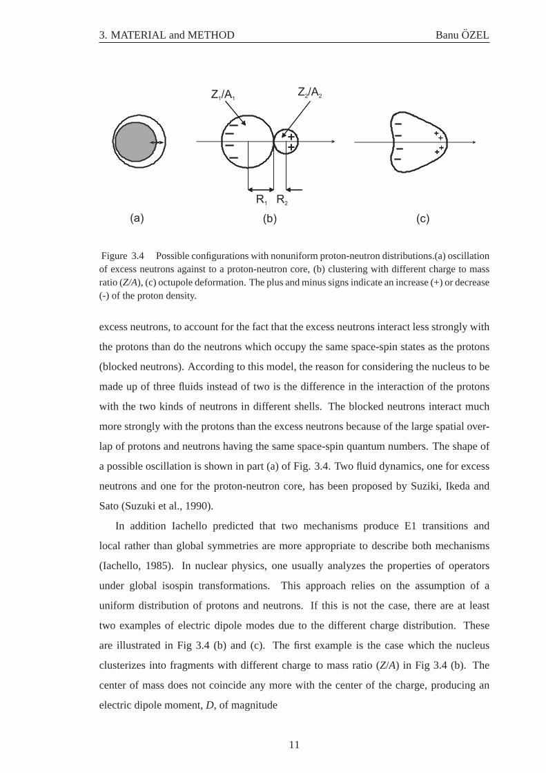
different explanations of producing low-lying E1 strength shown in Fig. 3.4. Especially
the hydrodynamical model by Mohan, Danos and Biedenhorn (Mohan et al., 1971) de-
scribe the PDR mode in nuclei. They use a three-fluid hydrodynamical model of nuclei,
the three fluids being the protons, the neutrons of the same orbitals as protons, and the
10
3. MATERIAL and METHOD BanuOZEL
++
++
+
+
++++
++
+
+
++
+
+
+
+
R1 R2
Z /A1 1Z /A2 2
(a) (b) (c)
Figure 3.4 Possible configurations with nonuniform proton-neutron distributions.(a) oscillationof excess neutrons against to a proton-neutron core, (b) clustering with different charge to massratio (Z/A), (c) octupole deformation. The plus and minus signs indicate an increase (+) or decrease(-) of the proton density.
excess neutrons, to account for the fact that the excess neutrons interact less strongly with
the protons than do the neutrons which occupy the same space-spin states as the protons
(blocked neutrons). According to this model, the reason for considering the nucleus to be
made up of three fluids instead of two is the difference in the interaction of the protons
with the two kinds of neutrons in different shells. The blocked neutrons interact much
more strongly with the protons than the excess neutrons because of the large spatial over-
lap of protons and neutrons having the same space-spin quantum numbers. The shape of
a possible oscillation is shown in part (a) of Fig. 3.4. Two fluid dynamics, one for excess
neutrons and one for the proton-neutron core, has been proposed by Suziki, Ikeda and
Sato (Suzuki et al., 1990).
In addition Iachello predicted that two mechanisms produce E1 transitions and
local rather than global symmetries are more appropriate to describe both mechanisms
(Iachello, 1985). In nuclear physics, one usually analyzes the properties of operators
under global isospin transformations. This approach relies on the assumption of a
uniform distribution of protons and neutrons. If this is not the case, there are at least
two examples of electric dipole modes due to the different charge distribution. These
are illustrated in Fig 3.4 (b) and (c). The first example is the case which the nucleus
clusterizes into fragments with different charge to mass ratio (Z/A) in Fig 3.4 (b). The
center of mass does not coincide any more with the center of the charge, producing an
electric dipole moment,D, of magnitude
11
3. MATERIAL and METHOD BanuOZEL
D = e2[(N−Z)/A]R0(A1/31 +41/3) (3.4)
for the example of alpha clustering. This dipole moment is not negligible and will
produce E1 transitions of considerable magnitude. The second mechanism is shown in
part (c) of Fig. 3.4. Consider the case in which the nucleus has a permanent octupole
deformation. This produces a dipole moment
D = 0.000687AZβ2β3(e f m), (3.5)
whereβ2 andβ3 are the quadrupole and octupole deformations.
For a final understanding we need microscopic models where the low-lying E1
strength occurs naturally. There are different approaches to predict a low-lying E1 reso-
nance in nuclei like microscopic density fluctuation theory (DFT) (Chambers et al., 1994)
or describing out-of-phase motion of neutrons against to protons including the effect
of neutron thickness (Van Isacker et al., 1992). These models usually overestimate the
B(E1) strength and always expect a rather simple direct correlation between the summed
strength and the neutron excess. In recent years a number of microscopic approaches
like QRPA (Oros et al., 1998; Col `o et al., 2000) and relativistic QRPA (Vretenar et al.,
2000; 2002; Paar et al., 2005) based on the relativistic Hartree-Bogoliubov model with
a density-dependent meson exchange (DD-ME) interaction, the QPM (Ryezayeva et al.,
2002) which goes beyond the RPA and includes the coupling to more complex configura-
tions. QPM calculations based on a Woods-Saxon ground state and a separable multipole
force for the residual interaction (Tsoneva et al., 2004) and the extended theory of finite
fermion systems (ETFFS) (Hartmann et al., 2004) have been used to calculate the PDR.
The predictions for the PDR differ substantially, in particular between nonrelativistic and
relativistic models.
12
3. MATERIAL and METHOD BanuOZEL
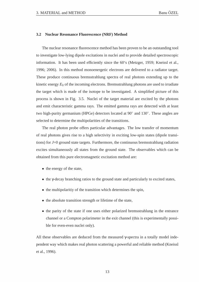
3.2 Nuclear Resonance Fluorescence (NRF) Method
The nuclear resonance fluorescence method has been proven to be an outstanding tool
to investigate low-lying dipole excitations in nuclei and to provide detailed spectroscopic
information. It has been used efficiently since the 60‘s (Metzger, 1959; Kneissl et al.,
1996; 2006). In this method monoenergetic electrons are delivered to a radiator target.
These produce continuous bremsstrahlung spectra of real photons extending up to the
kinetic energyE0 of the incoming electrons. Bremsstrahlung photons are used to irradiate
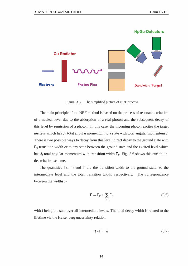
the target which is made of the isotope to be investigated. A simplified picture of this
process is shown in Fig. 3.5. Nuclei of the target material are excited by the photons
and emit characteristic gamma rays. The emitted gamma rays are detected with at least
two high-purity germanium (HPGe) detectors located at 90◦ and 130◦. These angles are
selected to determine the multipolarities of the transitions.
The real photon probe offers particular advantages. The low transfer of momentum
of real photons gives rise to a high selectivity in exciting low-spin states (dipole transi-
tions) forJ=0 ground state targets. Furthermore, the continuous bremsstrahlung radiation
excites simultaneously all states from the ground state. The observables which can be
obtained from this pure electromagnetic excitation method are:
• the energy of the state,
• theγ-decay branching ratios to the ground state and particularly to excited states,
• the multipolaritiy of the transition which determines the spin,
• the absolute transition strength or lifetime of the state,
• the parity of the state if one uses either polarized bremsstrahlung in the entrance
channel or a Compton polarimeter in the exit channel (this is experimentally possi-
ble for even-even nuclei only).
All these observables are deduced from the measuredγ-spectra in a totally model inde-
pendent way which makes real photon scattering a powerful and reliable method (Kneissl
et al., 1996).
13
3. MATERIAL and METHOD BanuOZEL
Photon FluxElectrons
HpGe-Detectors
Cu Radiator
Photon FluxElectrons
HpGe-Detectors
Cu Radiator
Sandwich Target
Figure 3.5 The simplified picture of NRF process
The main principle of the NRF method is based on the process of resonant excitation
of a nuclear level due to the absorption of a real photon and the subsequent decay of
this level by remission of a photon. In this case, the incoming photon excites the target
nucleus which hasJ0 total angular momentum to a state with total angular momentumJ.
There is two possible ways to decay from this level; direct decay to the ground state with
Γ0 transition width or to any state between the ground state and the excited level which
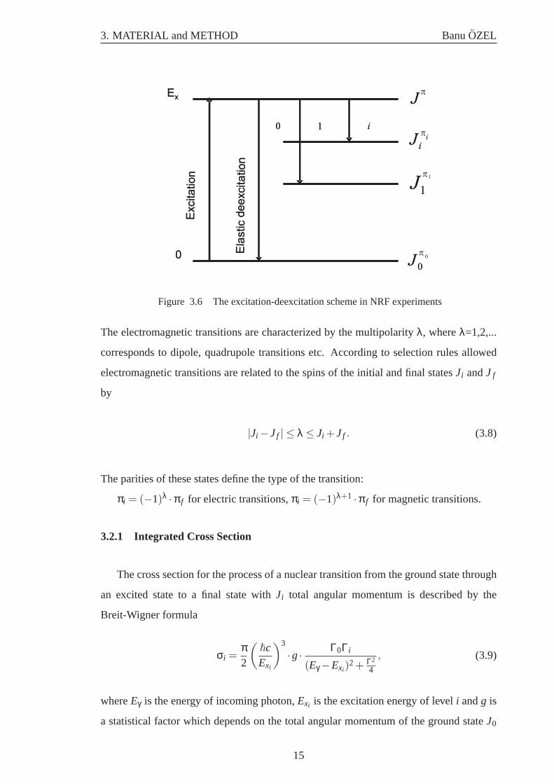
hasJi total angular momentum with transition widthΓi. Fig. 3.6 shows this excitation-
deexcitation scheme.
The quantitiesΓ0, Γi and Γ are the transition width to the ground state, to the
intermediate level and the total transition width, respectively. The correspondence
between the widths is
Γ = Γ0 + ∑i>0
Γi (3.6)
with i being the sum over all intermediate levels. The total decay width is related to the
lifetime via the Heisenberg uncertainty relation
τ∗Γ = ~ (3.7)
14
3. MATERIAL and METHOD BanuOZEL
Excita
tion
Ela
stic
dee
xcita
tion
0
Ex
iG
0G
1G
0
0J
1
1J
i
iJ
J
Excita
tion
Ela
stic
dee
xcita
tion
0
Ex
iG
0G
1G
0J
1J
i
iJ
Jp
p
p
p
Figure 3.6 The excitation-deexcitation scheme in NRF experiments
The electromagnetic transitions are characterized by the multipolarityλ, whereλ=1,2,...
corresponds to dipole, quadrupole transitions etc. According to selection rules allowed
electromagnetic transitions are related to the spins of the initial and final statesJi andJ f
by
|Ji −Jf | ≤ λ ≤ Ji +Jf . (3.8)
The parities of these states define the type of the transition:
πi = (−1)λ ·π f for electric transitions,πi = (−1)λ+1 ·π f for magnetic transitions.
3.2.1 Integrated Cross Section
The cross section for the process of a nuclear transition from the ground state through
an excited state to a final state withJi total angular momentum is described by the
Breit-Wigner formula
σi =π2
(
~cExi
)3
·g· Γ0Γi
(Eγ −Exi)2 + Γ2
4
, (3.9)
whereEγ is the energy of incoming photon,Exi is the excitation energy of leveli andg is
a statistical factor which depends on the total angular momentum of the ground stateJ0
15
3. MATERIAL and METHOD BanuOZEL
and the angular momentum of the excited levelJ
g =2J+12J0 +1
. (3.10)
The total cross section is given by the sum of partial cross sections of the decays all
possible final states.
σtotalabs = ∑
iσi
abs(Eγ) = ∑i
π2
(
~cExi
)3
·g· Γ0Γi
(Eγ −Exi)2 + Γ2
4
. (3.11)
When a nucleus which is initially at rest and in a ground state absorbs a primaryγ
quantum with the energyEγ, a part of the energy∆Erec is transferred to the nucleus as a
recoil because of the finite mass of the nucleus. The relation between the recoil energy
andEγ is Eγ = Ex +∆Erec, with
∆Erec =E2
γ
2Mc2 , (3.12)
whereM is the rest mass of the nucleus. The excited nucleus is not at rest any more, but
it is moving in the direction of primary photon beam. If during the short decay time to
the ground state a secondary photon is emitted, its energy will experience a Doppler shift
in addition to the recoil correction. Thus, the emitted photon will have a different energy
dependence on the emission angleθ with respect to the incomingγ-quantum, which
excites the nucleus
Eγ = Ex−E2
γ
2Mc2 [1−2cosθ]. (3.13)
If this energy is large compared to the width of the level, as is generally the case, then the
cross section for resonance absorption of the emitted photon by some another neighboring
nucleus becomes extremely small. This is a precondition to make the detection of emitted
photons with the NRF method possible at all.
Another important factor for NRF experiments which should be taken into account in
this formula is the thermal motion of atoms in the target. This motion causes a Doppler
16
3. MATERIAL and METHOD BanuOZEL
broadening of the absorption line width. If we assume that thethermal velocities of
nucleiν can be given as a Maxwell distribution (Bethe et al., 1937)
f (v) =
(
M2πkT
)1/2
exp
(
−Mv2
2kT
)
, (3.14)
whereM is the nuclear mass,k is the Boltzmann constant, andT the absolute temperature,
then the Doppler-broadened Breit-Wigner distribution
σiDBW(Eγ,T) = 2π
(
~cEx
)2
·g· Γ0
Γ· Γi
√π
2∆exp
(
−Eγ −Ex
∆
)2
, (3.15)
replaces Eq. (3.9). Here,∆ is the Doppler width
∆ =
(
Eγ
c
)
·(
2kTM
)1/2
. (3.16)
We can use this Doppler-broadened distribution to extract the partial cross sectionI i for
the population of level by integration of Eq. (3.15). over the complete solid angle
Ii =∫
σiDBW(Eγ,T)dEγ = π2 ·
(
~cEx
)
·g· Γ0Γi
Γ. (3.17)
In case of the elastic transitionΓ0 will be equal toΓi and Eq. (3.17) replace to
I0 = π2 ·(
~cEx
)
·g· Γ20
Γ. (3.18)
3.2.2 Transition Width and Transition Strength
The ground state decay width is proportional to the reduced transition probability
B(Πλ,Eγ)
Γ0 = 8π∞
∑Πλ=1
λ+1λ[(2λ+1)!!]2
·(
Eγ
~c
)2λ+1
· 2J0 +12J+1
B(Πλ,Eγ) ↑, (3.19)
17
3. MATERIAL and METHOD BanuOZEL
whereΠ = E for electric transitions andΠ=M for magnetic transitions. The NRF tech-
nique is selective on dipole transitions and to a lesser extent on quadrupole transitions
because of the small momentum transfer of the photons. The relations between reduced
transition strengths and ground state decay width are given for even-even nuclei in the
following
B(E1) ↑[e2 f m2]
= 9.554·10−4 ·g· Γ0
[meV]·(
MeVEx
)3
, (3.20)
B(M1) ↑[µ2
N]= 8.641·10−2 ·g· Γ0
[meV]·(
MeVEx
)3
, (3.21)
B(E2) ↑[e2 f m4]
= 1.245·103 ·g· Γ0
[meV]·(
MeVEx
)5
. (3.22)
The reduced transition probabilities for the decayB(Πλ;J → J0) = B(Πλ) ↓ and
B(Πλ;J0 → J) = B(Πλ) ↑differ by the statistical factor introduced in Eq. (3.10)
B(Πλ) ↑= 2J+12J0 +1
·B(Πλ) ↓ . (3.23)
It is useful to compare the reduced transition strength to the so-called Weisskopf
units, which represent a measure of the single-particle strength. It is given for electric
transitions by
B(Eλ)W.u. = B(Eλ) ↓= 14π
[
3λ+3
]2
(1.2A1/3)2λe2 f m2λ. (3.24)
3.2.3 Angular Distribution
The spins of the excited levels can be determined by measuring the angular distribu-
tions of the scattered photons with respect to the incoming photon beam. The general
18
3. MATERIAL and METHOD BanuOZEL
formula for the angular correlation functionW(θ) of the scattered photon can be given as
a sum of even Legendre polynomialsPλ(Θ):
W(θ) = ∑λ=0,2,4,...
Ai→ jλ ·A j→k
λ ·Pλ(cosθ), (3.25)
whereθ is the scattering angle between the direction of incident photon and the scattered
photon andPλ(cosθ)are Legendre polynomials of orderλ. The coefficientAi→ jλ describes
the photon in the entrance channel, and similarlyA j→kλ takes into account the resonantly
scattered photon.
Even-even nuclei always have ground state angular momentum and the parityJπ0=0+.
As a consequence, only levels with 1 or 2 can be excited in (γ,γ′) experiments on
even-even targets. The angular distribution of photons scattered of even-even nucleus
with ground state spin 0, representing the most favorable case, through a pure dipole
transition (spin sequence 0-1-0) is given by
W(θ)dipole =34· (1+cos2θ) (3.26)
and through a pure quadrupole transition (spin sequence 0-2-0) is given by
W(θ)quadrupole=54· (1−3cos2θ+4cos4θ) (3.27)
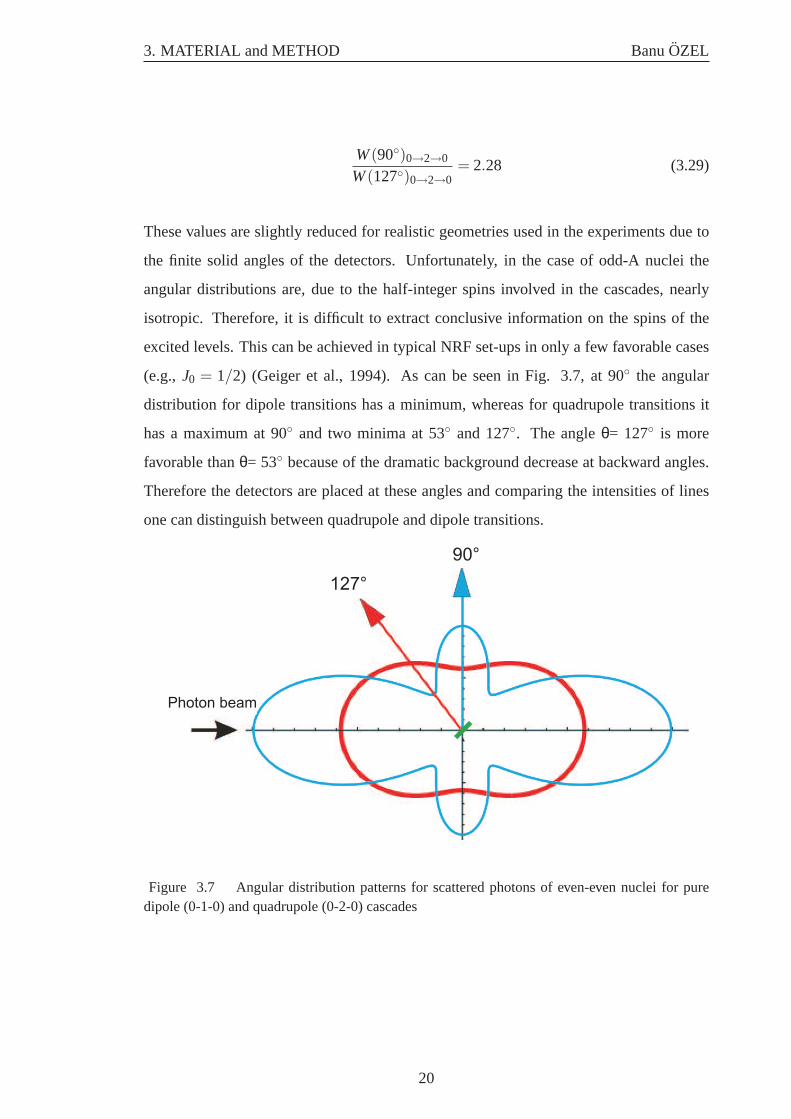
These angular distributions are depicted as polar diagrams in Fig. 3.7. It is evident
that for spin assignments in even even nuclei at least two different angles is need to be
measured. The most favorable configuration isθ = 90◦ and θ = 127◦. In the case of
even-even nuclei the predicted values for the ratio of measuredγ intensities at 90◦ and
127◦
W(90◦)0→1→0
W(127◦)0→1→0= 0.73 (3.28)
19
3. MATERIAL and METHOD BanuOZEL
W(90◦)0→2→0
W(127◦)0→2→0= 2.28 (3.29)
These values are slightly reduced for realistic geometries used in the experiments due to
the finite solid angles of the detectors. Unfortunately, in the case of odd-A nuclei the
angular distributions are, due to the half-integer spins involved in the cascades, nearly
isotropic. Therefore, it is difficult to extract conclusive information on the spins of the
excited levels. This can be achieved in typical NRF set-ups in only a few favorable cases
(e.g., J0 = 1/2) (Geiger et al., 1994). As can be seen in Fig. 3.7, at 90◦ the angular
distribution for dipole transitions has a minimum, whereas for quadrupole transitions it
has a maximum at 90◦ and two minima at 53◦ and 127◦. The angleθ= 127◦ is more
favorable thanθ= 53◦ because of the dramatic background decrease at backward angles.
Therefore the detectors are placed at these angles and comparing the intensities of lines
one can distinguish between quadrupole and dipole transitions.
Photon beam
90°
127°
Figure 3.7 Angular distribution patterns for scattered photons of even-even nuclei for puredipole (0-1-0) and quadrupole (0-2-0) cascades
20
3. MATERIAL and METHOD BanuOZEL
3.3 Photon Scattering Experiments at the S-DALINAC
3.3.1 The S-DALINAC
The present(γ,γ′) experiments ware performed at the superconducting Darmstadt
electron linear accelerator S-DALINAC (Richter, 1996). The S-DALINAC is historically
the third superconducting electron linac. It produced its first beam (Auerhammer et al.,
1992) in 1987 and went into full operation (Auerhammer et al. 1993; Aab et al., 1988) in
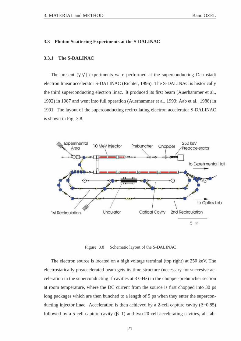
1991. The layout of the superconducting recirculating electron accelerator S-DALINAC
is shown in Fig. 3.8.
Figure 3.8 Schematic layout of the S-DALINAC
The electron source is located on a high voltage terminal (top right) at 250 keV. The
electrostatically preaccelerated beam gets its time structure (necessary for succesive ac-
celeration in the superconducting rf cavities at 3 GHz) in the chopper-prebuncher section
at room temperature, where the DC current from the source is first chopped into 30 ps
long packages which are then bunched to a length of 5 ps when they enter the supercon-
ducting injector linac. Acceleration is then achieved by a 2-cell capture cavity (β=0.85)
followed by a 5-cell capture cavity (β=1) and two 20-cell accelerating cavities, all fab-
21
3. MATERIAL and METHOD BanuOZEL
ricated from RRR=280 niobium and operated in liquid helium at 2 K.When leaving the
injector, the beam has an energy of up to 10 MeV and can either be used for low energy
experiments (the photon scattering) or it can be bent isochronously by 180◦ for injection
into the main linac. There, eight 20-cell cavities installed in four identical cryomodules
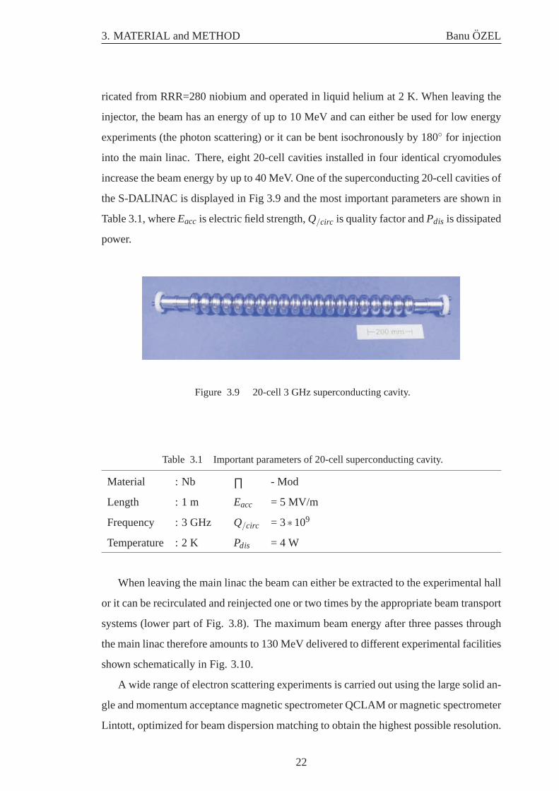
increase the beam energy by up to 40 MeV. One of the superconducting 20-cell cavities of
the S-DALINAC is displayed in Fig 3.9 and the most important parameters are shown in
Table 3.1, whereEacc is electric field strength,Q/circ is quality factor andPdis is dissipated
power.
Figure 3.9 20-cell 3 GHz superconducting cavity.
Table 3.1 Important parameters of 20-cell superconducting cavity.
Material : Nb ∏ - Mod
Length : 1 m Eacc = 5 MV/m
Frequency : 3 GHz Q/circ = 3∗109
Temperature : 2 K Pdis = 4 W
When leaving the main linac the beam can either be extracted to the experimental hall
or it can be recirculated and reinjected one or two times by the appropriate beam transport
systems (lower part of Fig. 3.8). The maximum beam energy after three passes through
the main linac therefore amounts to 130 MeV delivered to different experimental facilities
shown schematically in Fig. 3.10.
A wide range of electron scattering experiments is carried out using the large solid an-
gle and momentum acceptance magnetic spectrometer QCLAM or magnetic spectrometer
Lintott, optimized for beam dispersion matching to obtain the highest possible resolution.
22
3. MATERIAL and METHOD BanuOZEL
1
2
3
45
6
1 Real Photon
Free-Electron-Laser
High energie-beam physics
(e,e´x)-Experiment & 180°-Spectrometer
(e,e´)-Experiment
Compton scattering
of the nucleon
Laser-Experiment
7
11
22
33
4455
6
11 Real Photon
Free-Electron-Laser
High energie-beam physics
(e,e´x)-Experiment & 180°-Spectrometer
(e,e´)-Experiment
Compton scattering
of nucleon
Laser-Experiment
77
Accelerator Hall Experimental Hall
2
3
4
5
6
7
( , ´)g g
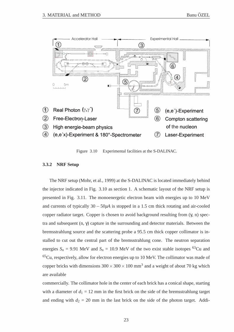
Figure 3.10 Experimental facilities at the S-DALINAC.
3.3.2 NRF Setup
The NRF setup (Mohr, et al., 1999) at the S-DALINAC is located immediately behind
the injector indicated in Fig. 3.10 as section 1. A schematic layout of the NRF setup is
presented in Fig. 3.11. The monoenergetic electron beam with energies up to 10 MeV
and currents of typically 30−50µAis stopped in a 1.5 cm thick rotating and air-cooled
copper radiator target. Copper is chosen to avoid background resulting from (γ, n) spec-
tra and subsequent (n,γ) capture in the surrounding and detector materials. Between the
bremsstrahlung source and the scattering probe a 95.5 cm thick copper collimator is in-
stalled to cut out the central part of the bremsstrahlung cone. The neutron separation
energiesSn = 9.91 MeV andSn = 10.9 MeV of the two exist stable isotopes63Cu and
65Cu, respectively, allow for electron energies up to 10 MeV. The collimator was made of
copper bricks with dimensions 300×300×100 mm3 and a weight of about 70 kg which
are available
commercially. The collimator hole in the center of each brick has a conical shape, starting
with a diameter ofd1 = 12 mm in the first brick on the side of the bremsstrahlung target
and ending withd2 = 20 mm in the last brick on the side of the photon target. Addi-
23
3. MATERIAL and METHOD BanuOZEL
HPGe detectors
+ BGO Shild
Collimator
e-
4th HPGe detector
3th HPGe detector
target
1 m
Radiator
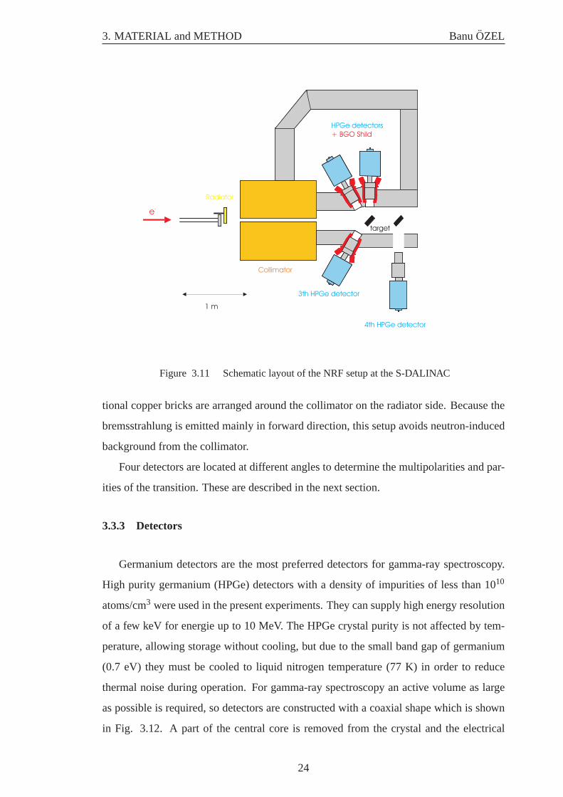
Figure 3.11 Schematic layout of the NRF setup at the S-DALINAC
tional copper bricks are arranged around the collimator on the radiator side. Because the
bremsstrahlung is emitted mainly in forward direction, this setup avoids neutron-induced
background from the collimator.
Four detectors are located at different angles to determine the multipolarities and par-
ities of the transition. These are described in the next section.
3.3.3 Detectors
Germanium detectors are the most preferred detectors for gamma-ray spectroscopy.
High purity germanium (HPGe) detectors with a density of impurities of less than 1010
atoms/cm3 were used in the present experiments. They can supply high energy resolution
of a few keV for energie up to 10 MeV. The HPGe crystal purity is not affected by tem-
perature, allowing storage without cooling, but due to the small band gap of germanium
(0.7 eV) they must be cooled to liquid nitrogen temperature (77 K) in order to reduce
thermal noise during operation. For gamma-ray spectroscopy an active volume as large
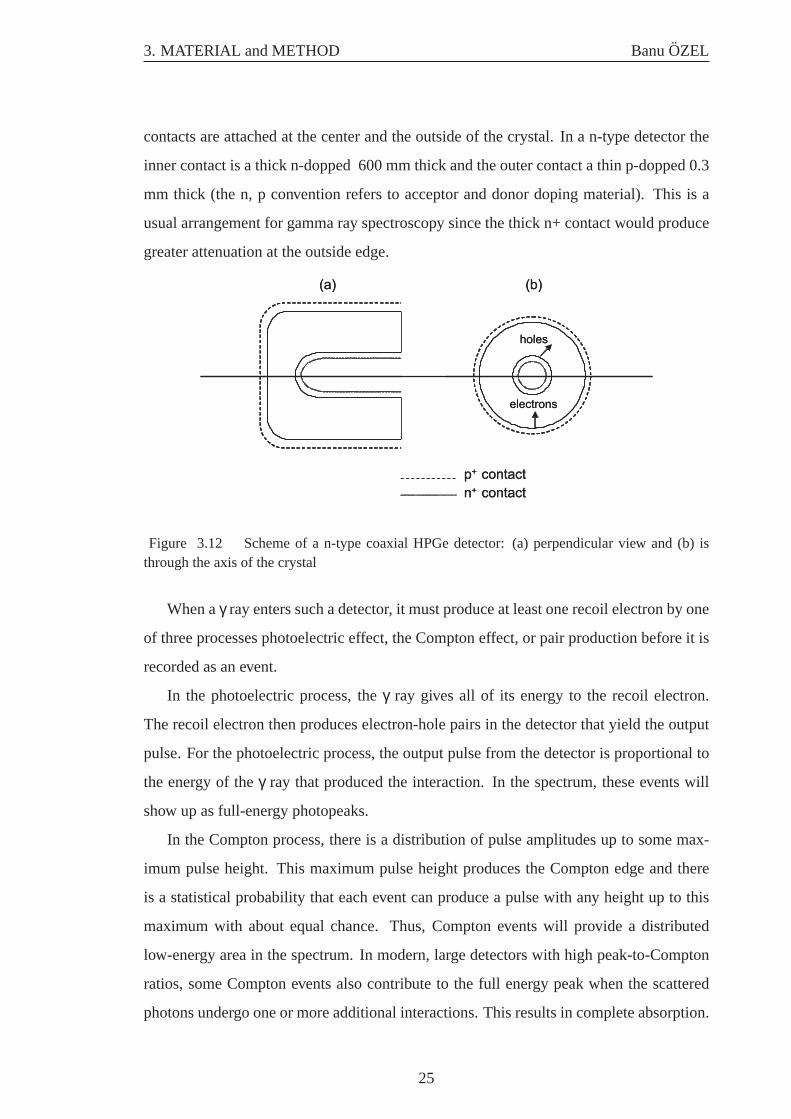
as possible is required, so detectors are constructed with a coaxial shape which is shown
in Fig. 3.12. A part of the central core is removed from the crystal and the electrical
24
3. MATERIAL and METHOD BanuOZEL
contacts are attached at the center and the outside of the crystal. In a n-type detector the
inner contact is a thick n-dopped 600 mm thick and the outer contact a thin p-dopped 0.3
mm thick (the n, p convention refers to acceptor and donor doping material). This is a
usual arrangement for gamma ray spectroscopy since the thick n+ contact would produce
greater attenuation at the outside edge.
p+ contact
n+ contact
electrons
holes
(a) (b)
p+ contact
n+ contact
electrons
holes
(a) (b)
Figure 3.12 Scheme of a n-type coaxial HPGe detector: (a) perpendicular view and (b) isthrough the axis of the crystal
When aγ ray enters such a detector, it must produce at least one recoil electron by one
of three processes photoelectric effect, the Compton effect, or pair production before it is
recorded as an event.
In the photoelectric process, theγ ray gives all of its energy to the recoil electron.
The recoil electron then produces electron-hole pairs in the detector that yield the output
pulse. For the photoelectric process, the output pulse from the detector is proportional to
the energy of theγ ray that produced the interaction. In the spectrum, these events will
show up as full-energy photopeaks.
In the Compton process, there is a distribution of pulse amplitudes up to some max-
imum pulse height. This maximum pulse height produces the Compton edge and there
is a statistical probability that each event can produce a pulse with any height up to this
maximum with about equal chance. Thus, Compton events will provide a distributed
low-energy area in the spectrum. In modern, large detectors with high peak-to-Compton
ratios, some Compton events also contribute to the full energy peak when the scattered
photons undergo one or more additional interactions. This results in complete absorption.
25
3. MATERIAL and METHOD BanuOZEL
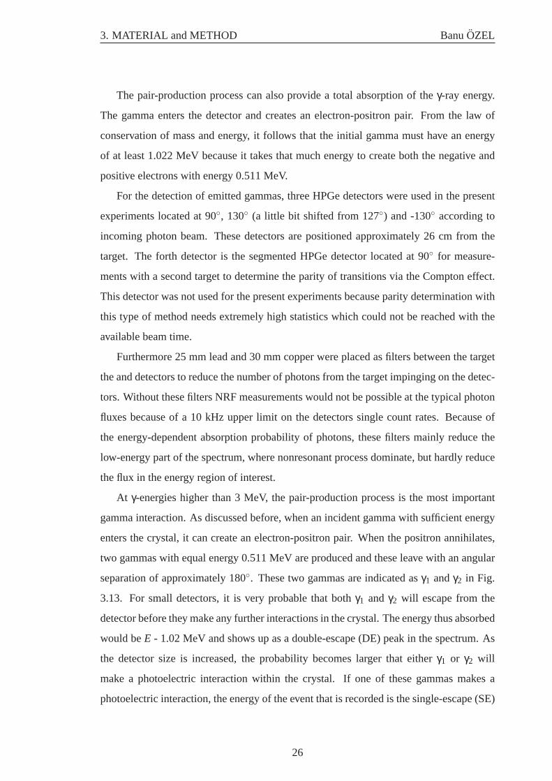
The pair-production process can also provide a total absorption of theγ-ray energy.
The gamma enters the detector and creates an electron-positron pair. From the law of
conservation of mass and energy, it follows that the initial gamma must have an energy
of at least 1.022 MeV because it takes that much energy to create both the negative and
positive electrons with energy 0.511 MeV.
For the detection of emitted gammas, three HPGe detectors were used in the present
experiments located at 90◦, 130◦ (a little bit shifted from 127◦) and -130◦ according to
incoming photon beam. These detectors are positioned approximately 26 cm from the
target. The forth detector is the segmented HPGe detector located at 90◦ for measure-
ments with a second target to determine the parity of transitions via the Compton effect.
This detector was not used for the present experiments because parity determination with
this type of method needs extremely high statistics which could not be reached with the
available beam time.
Furthermore 25 mm lead and 30 mm copper were placed as filters between the target
the and detectors to reduce the number of photons from the target impinging on the detec-
tors. Without these filters NRF measurements would not be possible at the typical photon
fluxes because of a 10 kHz upper limit on the detectors single count rates. Because of
the energy-dependent absorption probability of photons, these filters mainly reduce the
low-energy part of the spectrum, where nonresonant process dominate, but hardly reduce
the flux in the energy region of interest.
At γ-energies higher than 3 MeV, the pair-production process is the most important
gamma interaction. As discussed before, when an incident gamma with sufficient energy
enters the crystal, it can create an electron-positron pair. When the positron annihilates,
two gammas with equal energy 0.511 MeV are produced and these leave with an angular
separation of approximately 180◦. These two gammas are indicated asγ1 andγ2 in Fig.
3.13. For small detectors, it is very probable that bothγ1 and γ2 will escape from the
detector before they make any further interactions in the crystal. The energy thus absorbed
would beE - 1.02 MeV and shows up as a double-escape (DE) peak in the spectrum. As
the detector size is increased, the probability becomes larger that eitherγ1 or γ2 will
make a photoelectric interaction within the crystal. If one of these gammas makes a
photoelectric interaction, the energy of the event that is recorded is the single-escape (SE)
26
3. MATERIAL and METHOD BanuOZEL
Pair production
Annihilation
Ge Detector
Incident gamma
e-
e+
Pair production
Annihilation
Ge Detector
Incident gamma
e-
e+g
g1 g2
g1=g2= 511 keV
Figure 3.13 Principle of SE and DE.
peak. For even larger detectors, the probability of photoelectric interactions is further
increased and bothγ1 andγ2 could make photoelectric interactions within the crystal. If
bothγ1 andγ2 make photoelectric interactions, the total energy of the incident gamma is
absorbed within the crystal.
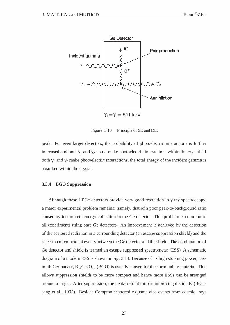
3.3.4 BGO Suppression
Although these HPGe detectors provide very good resolution inγ-ray spectroscopy,
a major experimental problem remains; namely, that of a poor peak-to-background ratio
caused by incomplete energy collection in the Ge detector. This problem is common to
all experiments using bare Ge detectors. An improvement is achieved by the detection
of the scattered radiation in a surrounding detector (an escape suppression shield) and the
rejection of coincident events between the Ge detector and the shield. The combination of
Ge detector and shield is termed an escape suppressed spectrometer (ESS). A schematic
diagram of a modern ESS is shown in Fig. 3.14. Because of its high stopping power, Bis-
muth Germanate, Bi4Ge3O12 (BGO) is usually chosen for the surrounding material. This
allows suppression shields to be more compact and hence more ESSs can be arranged
around a target. After suppression, the peak-to-total ratio is improving distinctly (Beau-
sang et al., 1995). Besides Compton-scatteredγ-quanta also events from cosmic rays
27
3. MATERIAL and METHOD BanuOZEL
Heavy metal collimator
Target
BGO Ge Crystal Liquid Nitrogen Dewar
Photomultiplier tubes Support frameHeavy metal collimator
Target
BGO Ge Crystal Liquid Nitrogen Dewar
Photomultiplier tubes Support frame
Figure 3.14 Typical construction of HPGe detector with BGO shield
4 5 60
4
8
Energy (MeV)
Counts
x 1
0-3
SE 11B
112Sn( , ´)g g
q = 130°
Figure 3.15 Measured spectra with BGO and without BGO
28

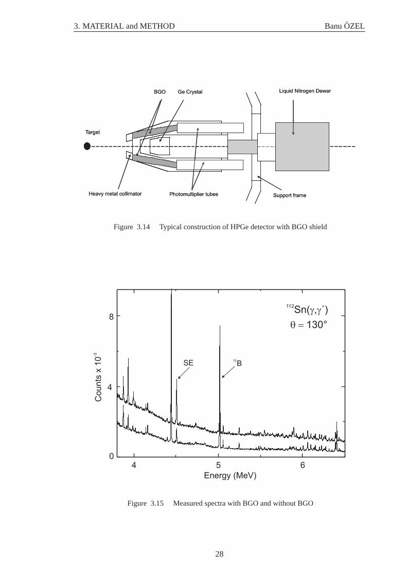
3. MATERIAL and METHOD BanuOZEL
contribute to the background in the spectrum. These events can also be suppressed by the
BGO shield. Moreover one can reduce significantly the SE and DE lines. The improve-
ment in the spectrum quality obtained by using of an ESS is demonstrated in Fig 3.15.
The figure shows the difference between the spectra which are taken with and without a
BGO shield. The background and the SE peak at 4.5 MeV from the strong line of11B at 5
MeV are distinctly reduced and the DE peak is completely suppressed by using the BGO
shield.
29
4. ANALYSIS and RESULTS BanuOZEL
4. ANALYSIS and RESULTS
4.1 Analysis of Resolved Transitions
4.1.1 Experimental Details
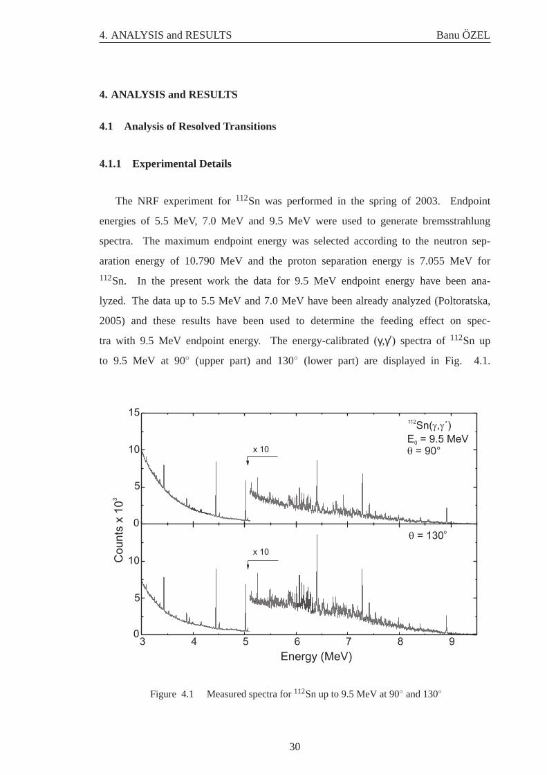
The NRF experiment for112Sn was performed in the spring of 2003. Endpoint
energies of 5.5 MeV, 7.0 MeV and 9.5 MeV were used to generate bremsstrahlung
spectra. The maximum endpoint energy was selected according to the neutron sep-
aration energy of 10.790 MeV and the proton separation energy is 7.055 MeV for
112Sn. In the present work the data for 9.5 MeV endpoint energy have been ana-
lyzed. The data up to 5.5 MeV and 7.0 MeV have been already analyzed (Poltoratska,
2005) and these results have been used to determine the feeding effect on spec-
tra with 9.5 MeV endpoint energy. The energy-calibrated (γ,γ′) spectra of112Sn up
to 9.5 MeV at 90◦ (upper part) and 130◦ (lower part) are displayed in Fig. 4.1.
3 4 5 6 7 8 90
10
0
5
10
15
Energy (MeV)
x 10
x 10
Counts
x 1
03
= 130qo
E = 9.5 MeV0
112Sn( , ´)g g
= 90°q
5
Figure 4.1 Measured spectra for112Sn up to 9.5 MeV at 90◦ and 130◦
30
4. ANALYSIS and RESULTS BanuOZEL
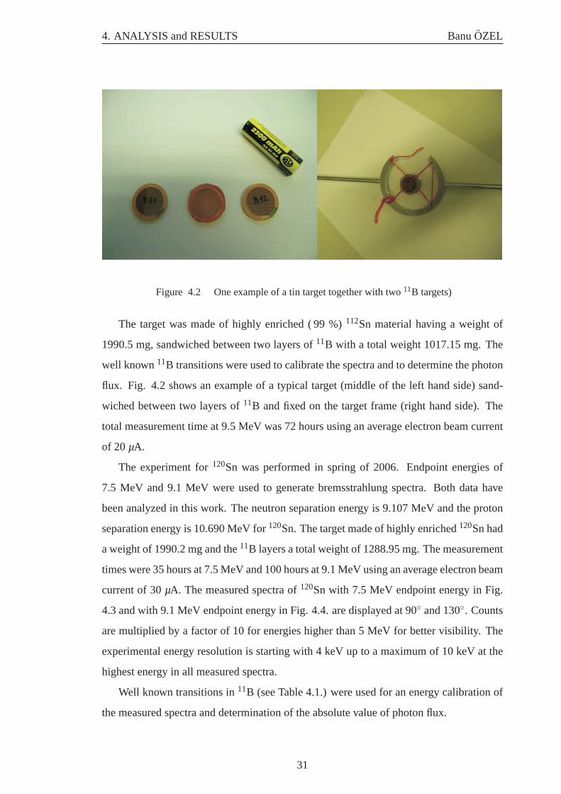
Figure 4.2 One example of a tin target together with two11B targets)
The target was made of highly enriched ( 99 %)112Sn material having a weight of
1990.5 mg, sandwiched between two layers of11B with a total weight 1017.15 mg. The
well known11B transitions were used to calibrate the spectra and to determine the photon
flux. Fig. 4.2 shows an example of a typical target (middle of the left hand side) sand-
wiched between two layers of11B and fixed on the target frame (right hand side). The
total measurement time at 9.5 MeV was 72 hours using an average electron beam current
of 20µA.
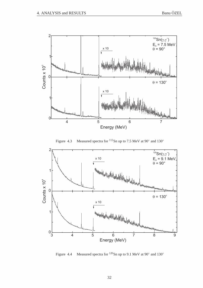
The experiment for120Sn was performed in spring of 2006. Endpoint energies of
7.5 MeV and 9.1 MeV were used to generate bremsstrahlung spectra. Both data have
been analyzed in this work. The neutron separation energy is 9.107 MeV and the proton
separation energy is 10.690 MeV for120Sn. The target made of highly enriched120Sn had
a weight of 1990.2 mg and the11B layers a total weight of 1288.95 mg. The measurement
times were 35 hours at 7.5 MeV and 100 hours at 9.1 MeV using an average electron beam
current of 30µA. The measured spectra of120Sn with 7.5 MeV endpoint energy in Fig.
4.3 and with 9.1 MeV endpoint energy in Fig. 4.4. are displayed at 90◦ and 130◦. Counts
are multiplied by a factor of 10 for energies higher than 5 MeV for better visibility. The
experimental energy resolution is starting with 4 keV up to a maximum of 10 keV at the
highest energy in all measured spectra.
Well known transitions in11B (see Table 4.1.) were used for an energy calibration of
the measured spectra and determination of the absolute value of photon flux.
31
4. ANALYSIS and RESULTS BanuOZEL
0
2
4 5 6 70
1
Energy (MeV)
1
Co
un
ts x
10
3
x 10
x 10E = 7.5 MeV0
120Sn( , ´)g g
= 90°q
= 130qo
Figure 4.3 Measured spectra for112Sn up to 7.5 MeV at 90◦ and 130◦
0
1
2
3 4 5 6 7 8 9
1
Energy (MeV)
Counts
x 1
04
E = 9.1 MeV0
120Sn( , ´)g g
= 90°q
= 130qo
0
x 10
x 10
Figure 4.4 Measured spectra for120Sn up to 9.1 MeV at 90◦ and 130◦
32
4. ANALYSIS and RESULTS BanuOZEL
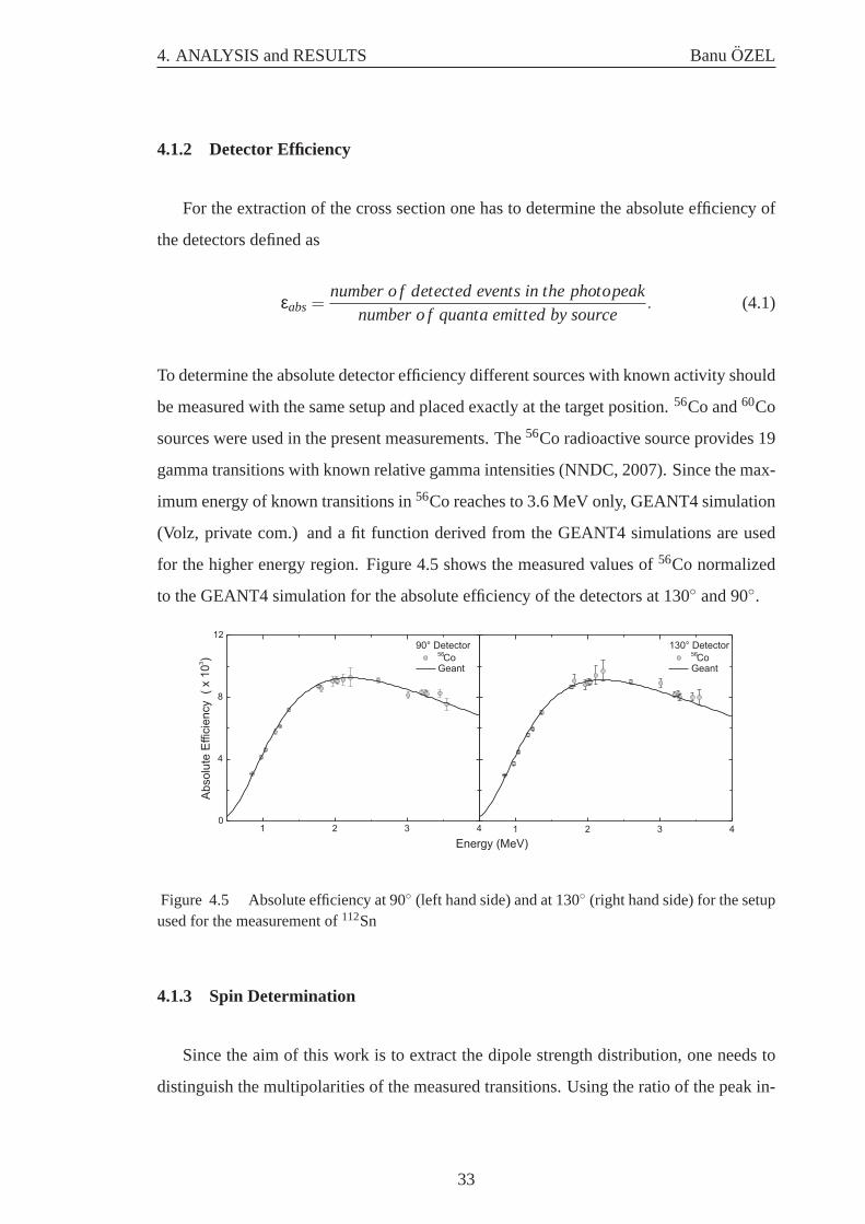
4.1.2 Detector Efficiency
For the extraction of the cross section one has to determine the absolute efficiency of
the detectors defined as
εabs=number o f detected events in the photopeak
number o f quanta emitted by source. (4.1)
To determine the absolute detector efficiency different sources with known activity should
be measured with the same setup and placed exactly at the target position.56Co and60Co
sources were used in the present measurements. The56Co radioactive source provides 19
gamma transitions with known relative gamma intensities (NNDC, 2007). Since the max-
imum energy of known transitions in56Co reaches to 3.6 MeV only, GEANT4 simulation
(Volz, private com.) and a fit function derived from the GEANT4 simulations are used
for the higher energy region. Figure 4.5 shows the measured values of56Co normalized
to the GEANT4 simulation for the absolute efficiency of the detectors at 130◦ and 90◦.
1 2 3 4
130° Detector56
CoGeant
1 2 3 40
4
8
12
Energy (MeV)
90° Detector56
CoGeant
Absolu
te E
ffic
iency (
x 1
0)
3
Figure 4.5 Absolute efficiency at 90◦ (left hand side) and at 130◦ (right hand side) for the setupused for the measurement of112Sn
4.1.3 Spin Determination
Since the aim of this work is to extract the dipole strength distribution, one needs to
distinguish the multipolarities of the measured transitions. Using the ratio of the peak in-
33
4. ANALYSIS and RESULTS BanuOZEL
0
1
2
2 4 6 80
1
2
Energy (MeV)
W(9
0°)
/ W
(130°)
112Sn = 1l
112Sn = 2l
120Sn = 1l
120Sn = 2l
11B
11B
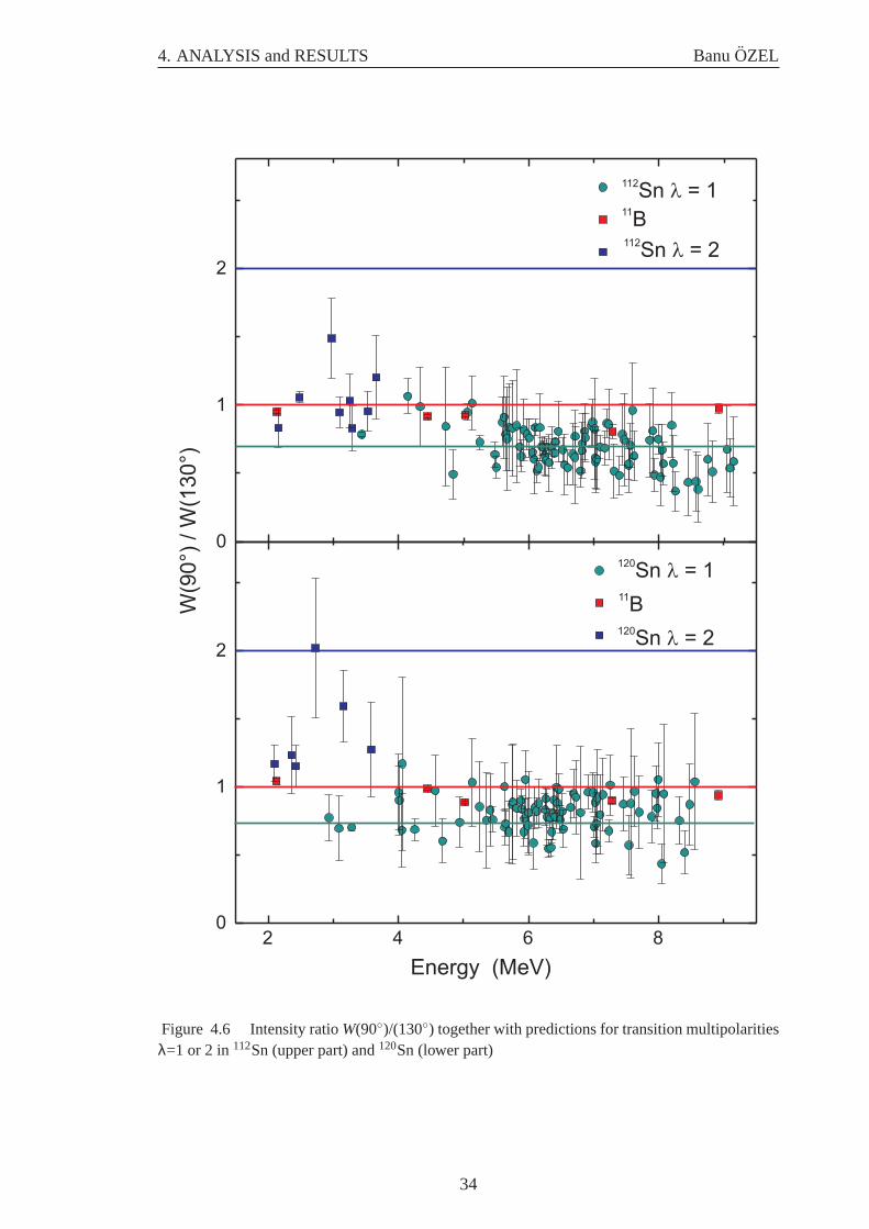
Figure 4.6 Intensity ratioW(90◦)/(130◦) together with predictions for transition multipolaritiesλ=1 or 2 in112Sn (upper part) and120Sn (lower part)
34
4. ANALYSIS and RESULTS BanuOZEL
tensities at different scattering angles one can extract themultipolarities of the observed
transitions. Figure 4.6 shows the intensity ratios of the transitions at 90◦ and 130◦ for
the 112Sn and120Sn isotopes. In the Fig. 4.6 the blue and green lines are the predicted
values for dipole transitions and quadrupole transitions, respectively. The red line at 1
indicates an isotropic distribution. The red squares correspond to11B transitions. These
transitions should be close to the isotropic line because of their half-integer spin. The
blue squares correspond to known (NNDC, 2007) quadrupole transitions. Because of
strong interaction in (γ,γ′) reaction, some 2+ states are also observed in the low energy
parts of the spectra. These transitions are closer to the isotropic line than expected for a
quadrupole transition because of the feeding effect from higher-energy levels discussed
below. The green points are dipole transitions for112Sn (upper part of the figure) and
120Sn (lower part of the figure). Most of the dipole transitions are observed the first time.
One can see that all observed ground state transitions above 5 MeV have dipole character.
4.1.4 Photon Flux and Integrated Cross Section
For a calculation of the B(E1) transition strength, one needs to know the photon flux
and the integrated cross section. The relation between photon flux and integrated cross
section is given by
Nγ(Ex,Eo) · εabs(Ex) =Ai
NTarget · I is ·Wi
e f f(θ)(4.2)
whereNγ(Ex,Eo) is the number of photons at an energyEx for a bremsstrahlungs spec-
trum with endpoint energyE0, εabs is the absolute efficiency at a given excitation energy,
Ai is the peak area of thei-th line in NRF spectrum andWie f f(θ) is the effective angular
correlation function. The product of the bremsstrahlung spectrum and the detector effi-
ciency was simulated using the program GEANT4 (Hasper, private com.) for the endpoint
energies of spectra. Since the GEANT4 simulations provide only the energy dependencie
of the flux but no absolute values, one has to normalize these to the experimental values
of 11B transitions using Eq. (4.2). In the calculation the branching ratios of boron lines
are taken to be account. The corresponding excitation energies, spin values of the excited
levels and integrated cross sections are given in Table 4.1 and the branching ratios of the
35
4. ANALYSIS and RESULTS BanuOZEL
Table 4.1 The transitions of11B, their spin values and integrated cross sections (NNDC, 2007)
Ex keV Jπ I0S (103eVfm2)
2124.69 12− 5.1(4)
4444.89 52− 16.3(6)
5020.31 32− 21.9(8)
7285.51 52+ 9.4(7)
8920.20 52− 28.6(14)
11B transitions are shown in Fig. 4.7.
Figure 4.8 shows the fit functions to the simulations ofNγ · εabs normalized with re-
spect to the11B lines for 112Sn (upper part) and120Sn (lower part). The upturned grey
triangles and the black triangles are the measured yields ofNγ ·εabs for the11B lines at 90◦
and 130◦, respectively. The grey lines show the fit functions of GEANT4 simulations for
the detector at 90◦ and the black lines this for the detector at 130◦. Once the photon flux is
8920.20
4444.89
7285.51
5020.31
2124.69
95
87 85.6 14.4
7.5
5.5
4.5
100100
100
0
Figure 4.7 Energies of11B transitions with branching ratios (NNDC, 2007)
known, one can calculate the integrated cross section for every transition. As mentioned
before the integrated cross section is proportional to the branching ratioΓ0/Γ, see Eq.
(3.18). Here it is assumed that all measured transitions exclusively decay to the ground
state, i.e, the quantity ofΓ0/Γ will be equal to 1. Usually this can be experimentally
checked for the branchings to the first excited 2+ state, but not for higher-lying states.
36
4. ANALYSIS and RESULTS BanuOZEL
Photon Energy (MeV)
2 4 6 8
102
103
104
102
103
104
130°
90°
Fit func. 90°
Fit func. 130°
130°
90°
Fit func. 90°
Fit func. 130°
Nx
(1/e
Vcm
)g
e2
Figure 4.8 Fit functions to the GEANT4 simulations forNγ · εabs normalized with respect tothe11B lines for112Sn (upper part) and120Sn (lower part)
37
4. ANALYSIS and RESULTS BanuOZEL
Furthermore a second assumption is that all excited states have Jπ=1−. This is justi-
fied because M1 transitions in spherical nuclei are of spin-flip nature and appear at higher
energies only (A. Richter, 1991). There is also an experimental test for the PDR in140Ce
where all the parities have been measured (N. Pietralla et al, 2002) and shown to be neg-
ative. Using the Eqs. (3.20)-(3.22), the B(E1), B(M1) and B(E2) transition probabilities
can be calculated.
4.1.5 Estimation of the Feeding Effect
The possibility of an indirect population of levels by feeding via inelastic transitions
from higher-lying states should be taken into account in the calculation of transition
strengths. A level can be populated directly by photoabsorption from the ground state
and also indirectly by decay from higher-lying states. This can cause an overestimation
on the real strength. As already mentioned in case of quadrupole transitions, strong feed-
ing can affect the spin assignment of transitions since the angular distributions of the
scattered photons become more isotropic. In this case one has to estimate the feeding
effect on the transition strengths. A possible way to investigate the amount of the feeding
is to compare the measured transition strengths at different endpoint energies.
The ratio of the measured transition strengths at 9.5 and 7 MeV endpoint energies for
112Sn is displayed in Fig. 4.9. Values larger than 1 indicate a feeding of the transitions.
This is the case for a number of transitions especially around 3 and 6.5 MeV. Therefore,
the transition strengths are corrected in the results of 9.5 MeV spectrum up to an energy
of 6.5 MeV. For ratios exceeding 1, the final values are taken from the measurement at
the lower endpoint energy. A spectrum for112Sn with 5.0 MeV endpoint energy is also
available. The comparison between the results of 7 MeV and 5 MeV was made in the
diploma thesis of Iryna Poltoratska (Poltoratska, 2005) and it was reported that there is
no feeding effect on 7 MeV spectrum.
The same calculations have also been performed for120Sn isotope. Fig. 4.10 shows
the ratio of the measured transition strengths at 9.1 and 7.5 MeV endpoint energies. As
seen from the figure obviously the case is different to the previous isotope. The feeding
is not observed on the measurement of120Sn up to 9.1 MeV. The differences between the
transition strengths for measurements up to 9.1 and 7.5 MeV are inside of error bars.
38
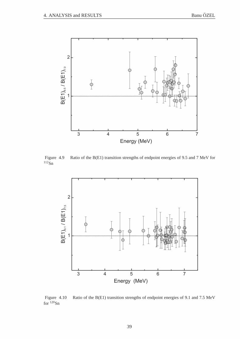
4. ANALYSIS and RESULTS BanuOZEL
3 4 5 6 7
1
2
Energy (MeV)
B(E
1)
/ B
(E1
)9.5
7.0
Figure 4.9 Ratio of the B(E1) transition strengths of endpoint energies of 9.5 and 7 MeV for112Sn
3 4 5 6 7
1
2
Energy (MeV)
B(E
1)
/ B
(E1)
9.1
7.5
Figure 4.10 Ratio of the B(E1) transition strengths of endpoint energies of 9.1 and 7.5 MeVfor 120Sn
39
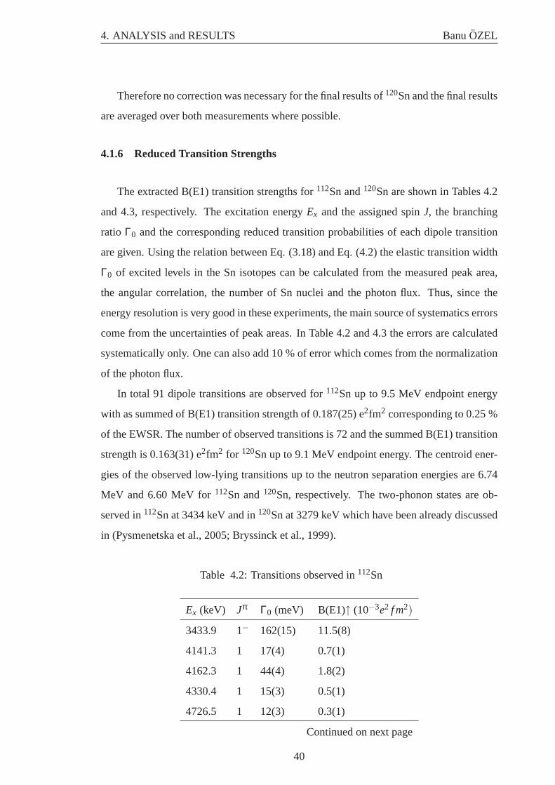
4. ANALYSIS and RESULTS BanuOZEL
Therefore no correction was necessary for the final results of120Sn and the final results
are averaged over both measurements where possible.
4.1.6 Reduced Transition Strengths
The extracted B(E1) transition strengths for112Sn and120Sn are shown in Tables 4.2
and 4.3, respectively. The excitation energyEx and the assigned spinJ, the branching
ratio Γ0 and the corresponding reduced transition probabilities of each dipole transition
are given. Using the relation between Eq. (3.18) and Eq. (4.2) the elastic transition width
Γ0 of excited levels in the Sn isotopes can be calculated from the measured peak area,
the angular correlation, the number of Sn nuclei and the photon flux. Thus, since the
energy resolution is very good in these experiments, the main source of systematics errors
come from the uncertainties of peak areas. In Table 4.2 and 4.3 the errors are calculated
systematically only. One can also add 10 % of error which comes from the normalization
of the photon flux.
In total 91 dipole transitions are observed for112Sn up to 9.5 MeV endpoint energy
with as summed of B(E1) transition strength of 0.187(25) e2fm2 corresponding to 0.25 %
of the EWSR. The number of observed transitions is 72 and the summed B(E1) transition
strength is 0.163(31) e2fm2 for 120Sn up to 9.1 MeV endpoint energy. The centroid ener-
gies of the observed low-lying transitions up to the neutron separation energies are 6.74
MeV and 6.60 MeV for112Sn and120Sn, respectively. The two-phonon states are ob-
served in112Sn at 3434 keV and in120Sn at 3279 keV which have been already discussed
in (Pysmenetska et al., 2005; Bryssinck et al., 1999).
Table 4.2: Transitions observed in112Sn
Ex (keV) Jπ Γ0 (meV) B(E1)↑(10−3e2 f m2)
3433.9 1− 162(15) 11.5(8)
4141.3 1 17(4) 0.7(1)
4162.3 1 44(4) 1.8(2)
4330.4 1 15(3) 0.5(1)
4726.5 1 12(3) 0.3(1)
Continued on next page
40
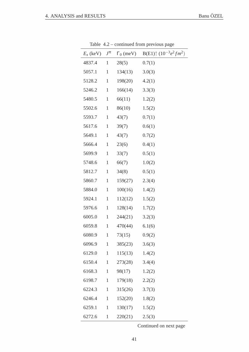
4. ANALYSIS and RESULTS BanuOZEL
Table 4.2 – continued from previous page
Ex (keV) Jπ Γ0 (meV) B(E1)↑(10−3e2 f m2)
4837.4 1 28(5) 0.7(1)
5057.1 1 134(13) 3.0(3)
5128.2 1 198(20) 4.2(1)
5246.2 1 166(14) 3.3(3)
5480.5 1 66(11) 1.2(2)
5502.6 1 86(10) 1.5(2)
5593.7 1 43(7) 0.7(1)
5617.6 1 39(7) 0.6(1)
5649.1 1 43(7) 0.7(2)
5666.4 1 23(6) 0.4(1)
5699.9 1 33(7) 0.5(1)
5748.6 1 66(7) 1.0(2)
5812.7 1 34(8) 0.5(1)
5860.7 1 159(27) 2.3(4)
5884.0 1 100(16) 1.4(2)
5924.1 1 112(12) 1.5(2)
5976.6 1 128(14) 1.7(2)
6005.0 1 244(21) 3.2(3)
6059.8 1 470(44) 6.1(6)
6080.9 1 73(15) 0.9(2)
6096.9 1 385(23) 3.6(3)
6129.0 1 115(13) 1.4(2)
6150.4 1 273(28) 3.4(4)
6168.3 1 98(17) 1.2(2)
6198.7 1 179(18) 2.2(2)
6224.3 1 315(26) 3.7(3)
6246.4 1 152(20) 1.8(2)
6259.1 1 130(17) 1.5(2)
6272.6 1 220(21) 2.5(3)
Continued on next page
41
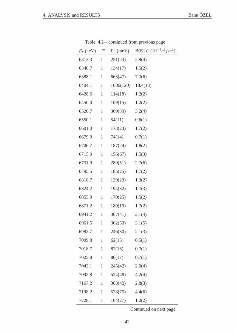
4. ANALYSIS and RESULTS BanuOZEL
Table 4.2 – continued from previous page
Ex (keV) Jπ Γ0 (meV) B(E1)↑(10−3e2 f m2)
6313.3 1 251(23) 2.9(4)
6348.7 1 134(17) 1.5(2)
6388.1 1 663(47) 7.3(6)
6404.1 1 1686(120) 18.4(13)
6428.6 1 114(18) 1.2(2)
6450.0 1 109(15) 1.2(2)
6520.7 1 309(33) 3.2(4)
6550.1 1 54(11) 0.6(1)
6601.0 1 173(23) 1.7(2)
6679.9 1 74(14) 0.7(1)
6706.7 1 187(24) 1.8(2)
6715.0 1 156(67) 1.5(3)
6731.9 1 289(51) 2.7(6)
6795.5 1 185(25) 1.7(2)
6818.7 1 139(23) 1.3(2)
6824.2 1 194(32) 1.7(3)
6855.9 1 170(25) 1.5(2)
6871.2 1 189(19) 1.7(2)
6941.2 1 367(41) 3.1(4)
6961.5 1 362(53) 3.1(5)
6982.7 1 246(30) 2.1(3)
7009.8 1 62(15) 0.5(1)
7018.7 1 82(16) 0.7(1)
7025.8 1 86(17) 0.7(1)
7043.1 1 245(42) 2.0(4)
7092.8 1 524(48) 4.2(4)
7167.2 1 363(42) 2.8(3)
7198.2 1 578(75) 4.4(6)
7228.1 1 164(27) 1.2(2)
Continued on next page
42
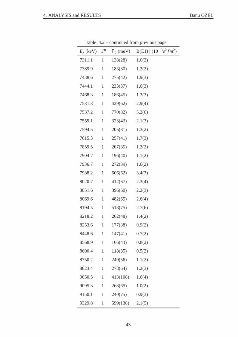
4. ANALYSIS and RESULTS BanuOZEL
Table 4.2 – continued from previous page
Ex (keV) Jπ Γ0 (meV) B(E1)↑(10−3e2 f m2)
7311.1 1 138(28) 1.0(2)
7389.9 1 183(30) 1.3(2)
7438.6 1 275(42) 1.9(3)
7444.1 1 233(37) 1.6(3)
7468.3 1 186(45) 1.3(3)
7531.3 1 429(62) 2.9(4)
7537.2 1 770(82) 5.2(6)
7559.1 1 323(43) 2.1(3)
7594.5 1 205(31) 1.3(2)
7615.3 1 257(41) 1.7(3)
7859.5 1 207(35) 1.2(2)
7904.7 1 196(40) 1.1(2)
7936.7 1 272(39) 1.6(2)
7988.2 1 606(62) 3.4(3)
8020.7 1 412(67) 2.3(4)
8051.6 1 396(60) 2.2(3)
8069.6 1 482(65) 2.6(4)
8194.5 1 518(75) 2.7(6)
8218.2 1 262(48) 1.4(2)
8253.6 1 177(38) 0.9(2)
8448.6 1 147(41) 0.7(2)
8568.9 1 166(43) 0.8(2)
8600.4 1 118(35) 0.5(2)
8750.2 1 249(56) 1.1(2)
8823.4 1 278(64) 1.2(3)
9050.5 1 413(108) 1.6(4)
9095.3 1 268(65) 1.0(2)
9150.1 1 240(75) 0.9(3)
9329.8 1 599(138) 2.1(5)
43
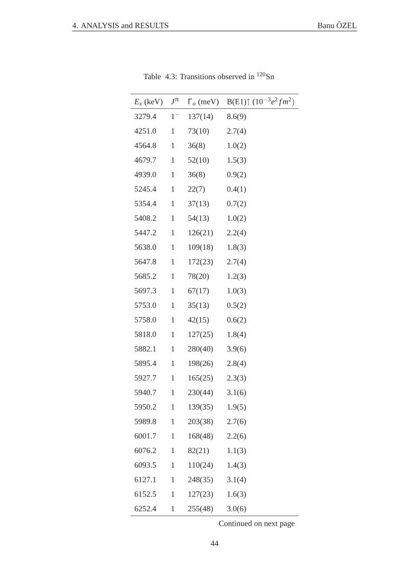
4. ANALYSIS and RESULTS BanuOZEL
Table 4.3: Transitions observed in120Sn
Ex (keV) Jπ Γo (meV) B(E1)↑(10−3e2 f m2)
3279.4 1− 137(14) 8.6(9)
4251.0 1 73(10) 2.7(4)
4564.8 1 36(8) 1.0(2)
4679.7 1 52(10) 1.5(3)
4939.0 1 36(8) 0.9(2)
5245.4 1 22(7) 0.4(1)
5354.4 1 37(13) 0.7(2)
5408.2 1 54(13) 1.0(2)
5447.2 1 126(21) 2.2(4)
5638.0 1 109(18) 1.8(3)
5647.8 1 172(23) 2.7(4)
5685.2 1 78(20) 1.2(3)
5697.3 1 67(17) 1.0(3)
5753.0 1 35(13) 0.5(2)
5758.0 1 42(15) 0.6(2)
5818.0 1 127(25) 1.8(4)
5882.1 1 280(40) 3.9(6)
5895.4 1 198(26) 2.8(4)
5927.7 1 165(25) 2.3(3)
5940.7 1 230(44) 3.1(6)
5950.2 1 139(35) 1.9(5)
5989.8 1 203(38) 2.7(6)
6001.7 1 168(48) 2.2(6)
6076.2 1 82(21) 1.1(3)
6093.5 1 110(24) 1.4(3)
6127.1 1 248(35) 3.1(4)
6152.5 1 127(23) 1.6(3)
6252.4 1 255(48) 3.0(6)
Continued on next page
44
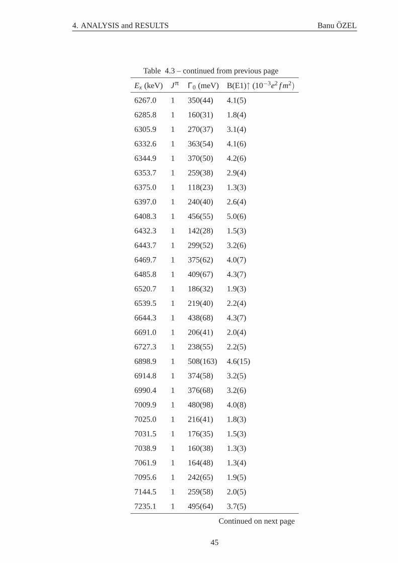
4. ANALYSIS and RESULTS BanuOZEL
Table 4.3 – continued from previous page
Ex (keV) Jπ Γ0 (meV) B(E1)↑(10−3e2 f m2)
6267.0 1 350(44) 4.1(5)
6285.8 1 160(31) 1.8(4)
6305.9 1 270(37) 3.1(4)
6332.6 1 363(54) 4.1(6)
6344.9 1 370(50) 4.2(6)
6353.7 1 259(38) 2.9(4)
6375.0 1 118(23) 1.3(3)
6397.0 1 240(40) 2.6(4)
6408.3 1 456(55) 5.0(6)
6432.3 1 142(28) 1.5(3)
6443.7 1 299(52) 3.2(6)
6469.7 1 375(62) 4.0(7)
6485.8 1 409(67) 4.3(7)
6520.7 1 186(32) 1.9(3)
6539.5 1 219(40) 2.2(4)
6644.3 1 438(68) 4.3(7)
6691.0 1 206(41) 2.0(4)
6727.3 1 238(55) 2.2(5)
6898.9 1 508(163) 4.6(15)
6914.8 1 374(58) 3.2(5)
6990.4 1 376(68) 3.2(6)
7009.9 1 480(98) 4.0(8)
7025.0 1 216(41) 1.8(3)
7031.5 1 176(35) 1.5(3)
7038.9 1 160(38) 1.3(3)
7061.9 1 164(48) 1.3(4)
7095.6 1 242(65) 1.9(5)
7144.5 1 259(58) 2.0(5)
7235.1 1 495(64) 3.7(5)
Continued on next page
45
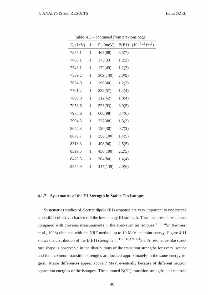
4. ANALYSIS and RESULTS BanuOZEL
Table 4.3 – continued from previous page
Ex (keV) Jπ Γ0 (meV) B(E1)↑(10−3e2 f m2)
7255.1 1 465(88) 3.5(7)
7460.1 1 175(33) 1.2(2)
7543.1 1 172(49) 1.1(3)
7569.2 1 309(140) 2.0(9)
7624.9 1 190(40) 1.2(3)
7701.2 1 229(57) 1.4(4)
7889.0 1 312(62) 1.8(4)
7958.6 1 523(93) 3.0(5)
7975.6 1 606(98) 3.4(6)
7994.5 1 237(48) 1.3(3)
8044.3 1 120(30) 0.7(2)
8079.7 1 258(100) 1.4(5)
8318.3 1 498(96) 2.5(5)
8399.5 1 450(100) 2.2(5)
8478.3 1 304(80) 1.4(4)
8554.9 1 447(139) 2.0(6)
4.1.7 Systematics of the E1 Strength in Stable Tin Isotopes
Systematics studies of electric dipole (E1) response are very important to understand
a possible collective character of the low-energy E1 strength. Thus, the present results are
compared with previous measurements in the even-even tin isotopes116,124Sn (Govaert
et al., 1998) obtained with the NRF method up to 10 MeV endpoint energy. Figure 4.11
shows the distribution of the B(E1) strengths in112,116,120,124Sn. A resonance-like struc-
ture shape is observable in the distributions of the transition strengths for every isotope
and the maximum transition strengths are located approximately in the same energy re-
gion. Major differences appear above 7 MeV, eventually because of different neutron
separation energies of the isotopes. The summed B(E1) transition strengths and centroid
46
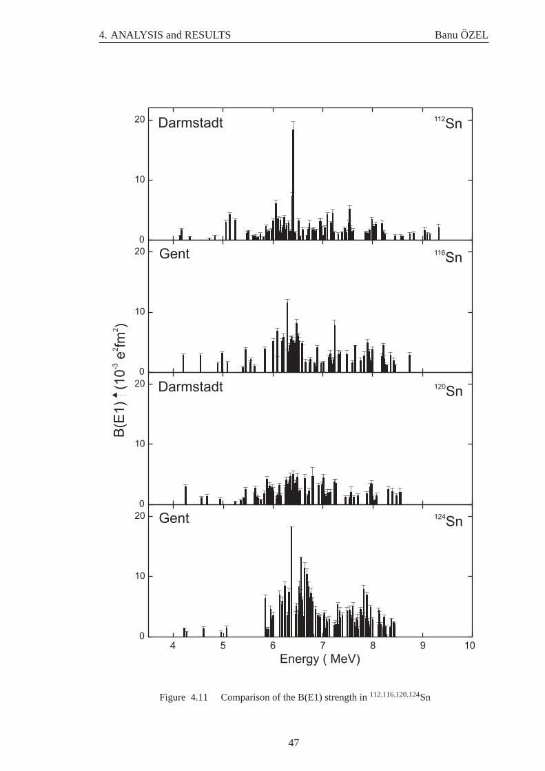
4. ANALYSIS and RESULTS BanuOZEL
0
10
20
0
10
20
0
10
20
0
10
20
B(E
1)
(1
0e
fm)
-32
2
4 5 6 7 8 9 10
Energy ( MeV)
Darmstadt
Darmstadt
Gent
Gent
116Sn
120Sn
124Sn
112Sn
Figure 4.11 Comparison of the B(E1) strength in112,116,120,124Sn
47
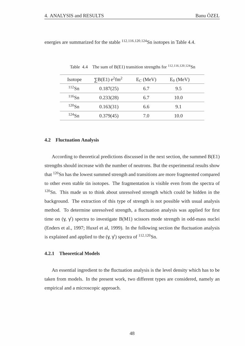
4. ANALYSIS and RESULTS BanuOZEL
energies are summarized for the stable112,116,120,124Sn isotopes in Table 4.4.
Table 4.4 The sum of B(E1) transition strengths for112,116,120,124Sn
Isotope ∑B(E1) e2fm2 EC (MeV) E0 (MeV)
112Sn 0.187(25) 6.7 9.5
116Sn 0.233(28) 6.7 10.0
120Sn 0.163(31) 6.6 9.1
124Sn 0.379(45) 7.0 10.0
4.2 Fluctuation Analysis
According to theoretical predictions discussed in the next section, the summed B(E1)
strengths should increase with the number of neutrons. But the experimental results show
that120Sn has the lowest summed strength and transitions are more fragmented compared
to other even stable tin isotopes. The fragmentation is visible even from the spectra of
120Sn. This made us to think about unresolved strength which could be hidden in the
background. The extraction of this type of strength is not possible with usual analysis
method. To determine unresolved strength, a fluctuation analysis was applied for first
time on (γ, γ′) spectra to investigate B(M1) scissors mode strength in odd-mass nuclei
(Enders et al., 1997; Huxel et al, 1999). In the following section the fluctuation analysis
is explained and applied to the (γ,γ′) spectra of112,120Sn.
4.2.1 Theoretical Models
An essential ingredient to the fluctuation analysis is the level density which has to be
taken from models. In the present work, two different types are considered, namely an
empirical and a microscopic approach.
48
4. ANALYSIS and RESULTS BanuOZEL
4.2.1.1 Back-Shifted Fermi Gas Model
Nuclear Level Densities (NLD) are important quantities in nuclear physics. For ex-
ample predicting the distribution of all the excited levels in nuclei helps to understand
this complicated quantum system. Besides, the NLD represent very important ingredients
in statistical model calculation of nuclear reactions cross sections which are needed for
many application in astrophysics and also fission or fusion reactor designs.In the present
work NLD are needed to determine the nonresonant background in (γ,γ′) spectra.
Most of the calculations of NLD are modifications and extensions of the Fermi gas
model including pairing and shell effects in a semi-empirical way (Gilbert, 1965), the
so-called back-shifted Fermi gas model (BSFG). The NLD dependence on energyEx and
spinJ is given in a separable form
ρ(Ex,J,π) =12
ρ(Ex) f (J) (4.3)
f (J) = exp[− J2
2σ2 ]−exp[−(J+1)2
2σ2 ]. (4.4)
The factor 1/2 in Eq. (4.3) results from the assumption of parity independence.
In the BSFG model (Gilbert, 1965) the energy part is given by
ρ(Ex) =exp[2
√
a(Ex−E1)]
12√
2σa1/4(Ex−E1)5/4. (4.5)
Hereσ is the spin cut-off parameter which depends on the rigid-body moment of inertia
of the nucleus. The formula is given by (Zhongfu, 1991)
σ2 = 0.0146A5/31+√
1+4a(Ex−E1)
2a(4.6)
whereE1 is the energy backshift anda is the NLD parameter in MeV−1. The quantity
a represents the shell effect taken to be independent of the energy. It means that the
shell effect plays a role at higher energies in the same way as at low energies. However,
49
4. ANALYSIS and RESULTS BanuOZEL
microscopic calculations of the NLD show that the shell effects are stronger at low
energies. Thus, an energy dependent description was needed to define fora parameter
which includes the quenching of the shell effect (Ignatyuk et al.,1975; 1979),
a(Ex,Z,N) = a[1+S(Z,N)−∆
Ex−E2 f (Ex−E2)]. (4.7)
Here,a is the asymptotic value of thea parameter
a = αA+βA2/3 (4.8)
The functionf has been proposed (Ignatyuk et al.,1975; Rauscher et al.,1997) to have the
following term
f (Ex−E2) = 1−exp[−γ(Ex−E2)]. (4.9)
In these calculationsα, γ, β are the free parameters which can be determined by fitting to
experimental data. In Eq.(4.7),S(Z, N)is given as a shell correction and is defined by
S(Z,N) = Mexp−MLD, (4.10)
whereMexp is the experimental mass andMLD is the mass calculated with a macroscopic
liquid-drop formula.
The following equation gives the total number of levels as a function of excitation
energyEx,
N0(Ex,J) =∫ Ex
0ρ(E,J)dE. (4.11)
Finally, the mean level spacing〈D〉=1/ρ in an energy interval [Eax , Ebx ] can be expressed
as (Kalmykov, 2004)
50
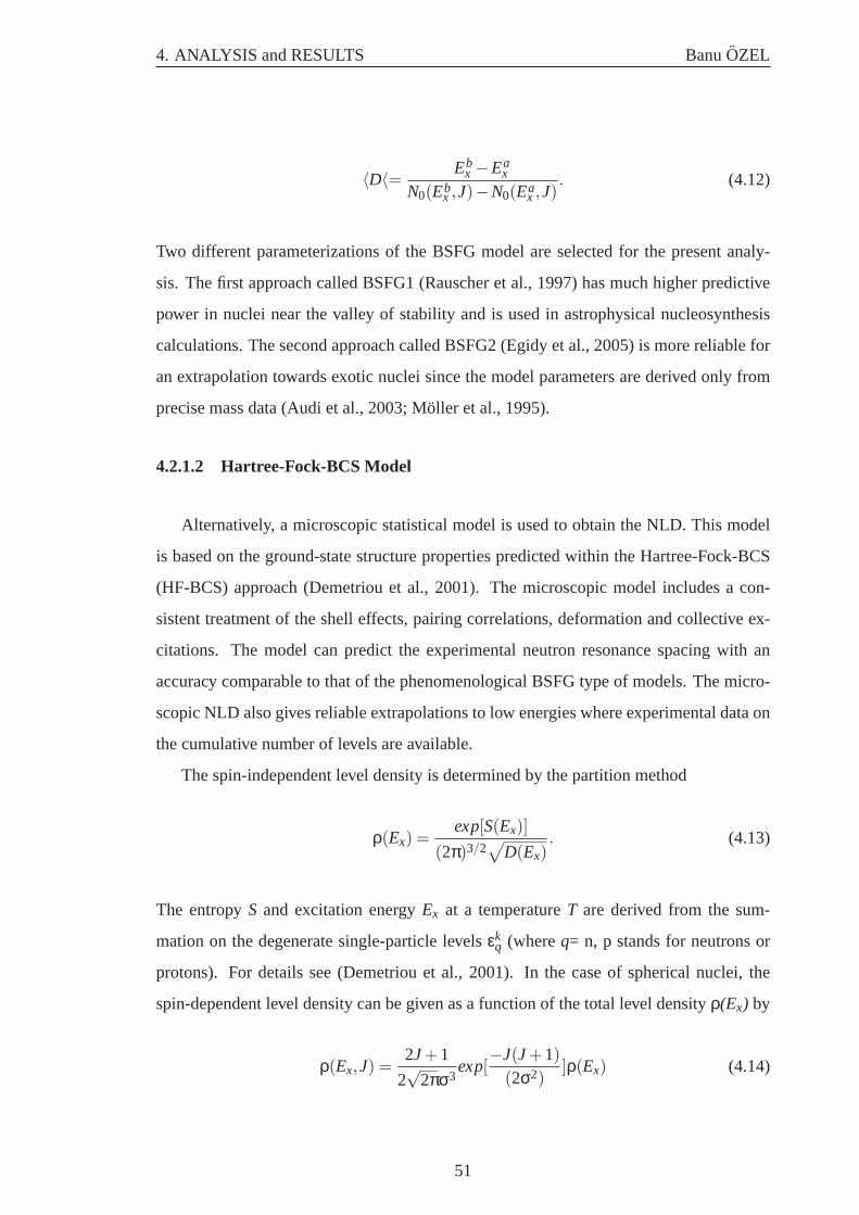
4. ANALYSIS and RESULTS BanuOZEL
〈D〈= Ebx −Ea
x
N0(Ebx ,J)−N0(Ea
x ,J). (4.12)
Two different parameterizations of the BSFG model are selected for the present analy-
sis. The first approach called BSFG1 (Rauscher et al., 1997) has much higher predictive
power in nuclei near the valley of stability and is used in astrophysical nucleosynthesis
calculations. The second approach called BSFG2 (Egidy et al., 2005) is more reliable for
an extrapolation towards exotic nuclei since the model parameters are derived only from
precise mass data (Audi et al., 2003; Moller et al., 1995).
4.2.1.2 Hartree-Fock-BCS Model
Alternatively, a microscopic statistical model is used to obtain the NLD. This model
is based on the ground-state structure properties predicted within the Hartree-Fock-BCS
(HF-BCS) approach (Demetriou et al., 2001). The microscopic model includes a con-
sistent treatment of the shell effects, pairing correlations, deformation and collective ex-
citations. The model can predict the experimental neutron resonance spacing with an
accuracy comparable to that of the phenomenological BSFG type of models. The micro-
scopic NLD also gives reliable extrapolations to low energies where experimental data on
the cumulative number of levels are available.
The spin-independent level density is determined by the partition method
ρ(Ex) =exp[S(Ex)]
(2π)3/2√
D(Ex). (4.13)
The entropyS and excitation energyEx at a temperatureT are derived from the sum-
mation on the degenerate single-particle levelsεkq (whereq= n, p stands for neutrons or
protons). For details see (Demetriou et al., 2001). In the case of spherical nuclei, the
spin-dependent level density can be given as a function of the total level densityρ(Ex) by
ρ(Ex,J) =2J+1
2√
2πσ3exp[
−J(J+1)
(2σ2)]ρ(Ex) (4.14)
51
4. ANALYSIS and RESULTS BanuOZEL
and spin cut-off parameter for the spherical nuclei is given by
σ2(T) =12 ∑
q=n,p∑k
mk2
q sech2(Ek
q
2T) (4.15)
which is obtained from the summation on the angular momentum projectionmkq. Here,
Ekq is the quasiparticle energy which depends on the single particle levels, the BCS gap
parameter and the chemical potential as a function of the pairing strength. The HF calcu-
lations are fit to the full set of measured masses (Tondeur et al., 2000; Goriely et al., 2001)
for the determination of the nucleon interaction. This should make the corresponding HF
predictions particularly reliable (Demetriou et al., 2001).
4.2.2 Fluctuation Analysis Method
The fluctuation analysis method was originally established forβ-delayed particle
emission spectra (Hansen, 1979), subsequently used for the giant resonant spectra from
electron scattering (Muller et al., 1982; Kilgus et al., 1987) and also applied success-
fully to γ-ray spectra to search for unresolved M1 strength in deformed odd-mass nuclei
(Enders et al., 1997; Huxel et al., 1999).
The method is applicable in the region where the mean level spacing〈D〉 is smaller
than the experimental energy resolution∆E and at the same time the mean level width
〈Γ〉 is smaller than〈D〉 and∆E, i.e.
〈Γ〉 ≤ 〈D〉 < ∆E (4.16)
The case of〈Γ〉 > 〈D〉 is called Ericson fluctuations (Ericson, 1960) which stem from the
coherent overlap of excitations whose line widths〈Γ〉 exceed the average level spacing.
Two assumptions are used for the calculation of experimental level densities. Because
of strong configuration mixing of levels with same spin and parity in a highly excited
nucleus, the probability for a certain spacing between neighboring states is assumed to
follow the Wigner distribution (Wigner, 1965)
52
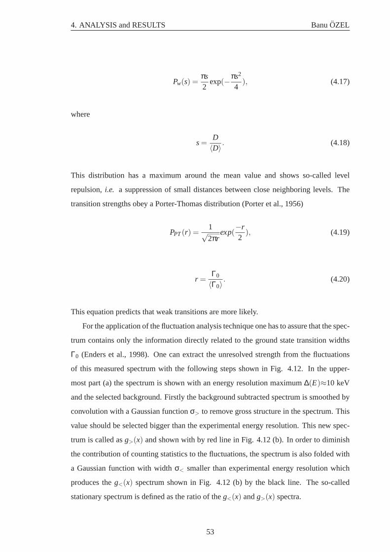
4. ANALYSIS and RESULTS BanuOZEL
Pw(s)=πs2
exp(−πs2
4), (4.17)
where
s=D〈D〉 . (4.18)
This distribution has a maximum around the mean value and shows so-called level
repulsion,i.e. a suppression of small distances between close neighboring levels. The
transition strengths obey a Porter-Thomas distribution (Porter et al., 1956)
PPT(r) =1√2πr
exp(−r2
), (4.19)
r =Γ0
〈Γ0〉. (4.20)
This equation predicts that weak transitions are more likely.
For the application of the fluctuation analysis technique one has to assure that the spec-
trum contains only the information directly related to the ground state transition widths
Γ0 (Enders et al., 1998). One can extract the unresolved strength from the fluctuations
of this measured spectrum with the following steps shown in Fig. 4.12. In the upper-
most part (a) the spectrum is shown with an energy resolution maximum∆(E)≈10 keV
and the selected background. Firstly the background subtracted spectrum is smoothed by
convolution with a Gaussian functionσ> to remove gross structure in the spectrum. This
value should be selected bigger than the experimental energy resolution. This new spec-
trum is called asg>(x) and shown with by red line in Fig. 4.12 (b). In order to diminish
the contribution of counting statistics to the fluctuations, the spectrum is also folded with
a Gaussian function with widthσ< smaller than experimental energy resolution which
produces theg<(x) spectrum shown in Fig. 4.12 (b) by the black line. The so-called
stationary spectrum is defined as the ratio of theg<(x) andg>(x) spectra.
53
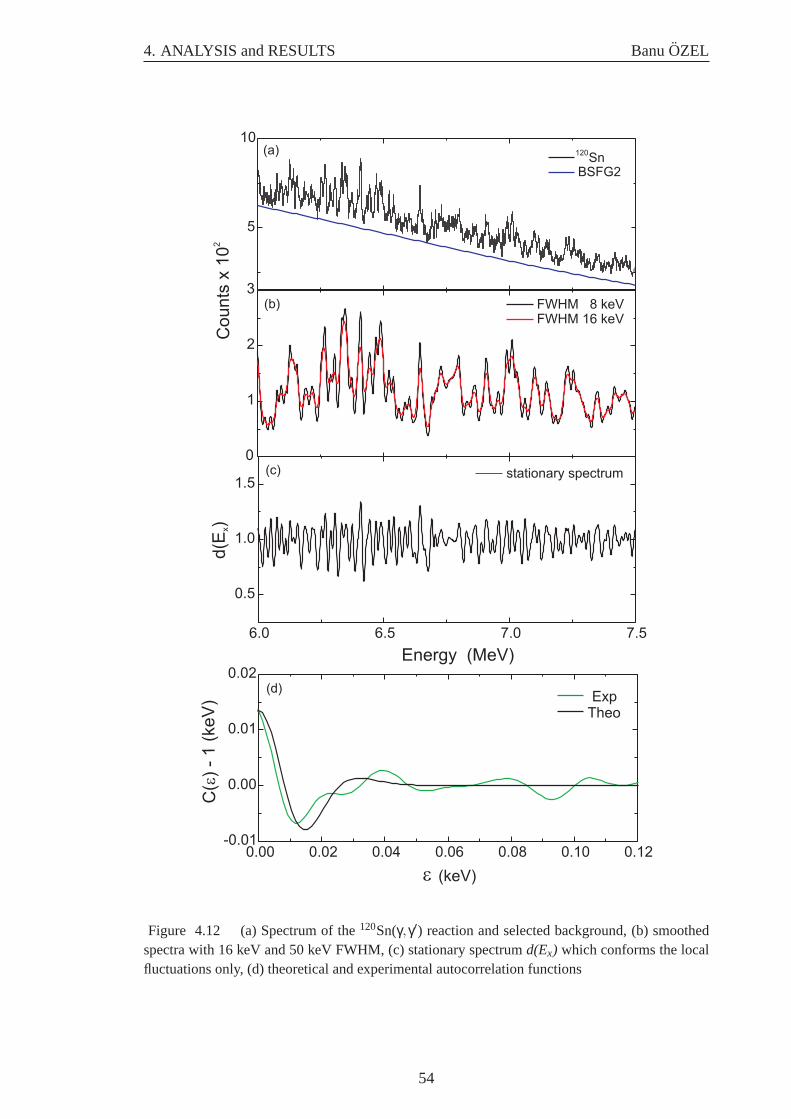
4. ANALYSIS and RESULTS BanuOZEL
5
10120
SnBSFG2
0
1
2
3FWHM 8 keVFWHM 16 keV
6.0 6.5 7.0 7.5
0.5
1.0
1.5stationary spectrum
Energy (MeV)
0.00 0.02 0.04 0.06 0.08 0.10 0.12-0.01
0.00
0.01
0.02
(keV)
C(
) -
1(k
eV
)e
e
Co
un
ts x
10
2
ExpTheo
(a)
(b)
(c)
(d)
d(E
)x
Figure 4.12 (a) Spectrum of the120Sn(γ,γ′) reaction and selected background, (b) smoothedspectra with 16 keV and 50 keV FWHM, (c) stationary spectrumd(Ex) which conforms the localfluctuations only, (d) theoretical and experimental autocorrelation functions
54
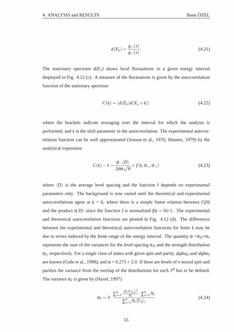
4. ANALYSIS and RESULTS BanuOZEL
d(Ex) =g<(x)g>(x)
. (4.21)
The stationary spectrumd(Ex) shows local fluctuations in a given energy interval
displayed in Fig. 4.12 (c). A measure of the fluctuations is given by the autocorrelation
function of the stationary spectrum
C(ε) = 〈d(Ex)d(Ex + ε)〉 (4.22)
where the brackets indicate averaging over the interval for which the analysis is
performed, andε is the shift parameter in the autocorrelation. The experimental autocor-
relation function can be well approximated (Jonson et al., 1976; Hansen, 1979) by the
analytical expression
C(ε)−1 =α · 〈D〉2σα
√π× f (ε,σ>,σ<) (4.23)
where 〈D〉 is the average level spacing and the function f depends on experimental
parameters only. The background is now varied until the theoretical and experimental
autocorrelations agree atε = 0, where there is a simple linear relation betweenC(0)
and the productα〈D〉 since the functionf is normalizedf(ε = 0)=1. The experimental
and theoretical autocorrelation functions are plotted in Fig. 4.12 (d). The differences
between the experimental and theoretical autocorrelation functions for finiteε may be
due to errors induced by the finite range of the energy interval. The quantityα =αD+αI
represents the sum of the variances for the level spacingαD and the strength distribution
αI , respectively. For a single class of states with given spin and parity, alphaD and alphaI
are known (Guhr et al., 1998), andα = 0.273 + 2.0. If there are levels ofn mixed spin and
parities the variance from the overlap of the distributions for eachJπ has to be defined.
The varianceαI is given by (Huxel, 1997)
αI = 3·∑n
i=1(Ni〈Γ0〉i)2
Ni·∑n
i=1 Ni
∑ni=1 Ni〈Γ0〉i
(4.24)
55
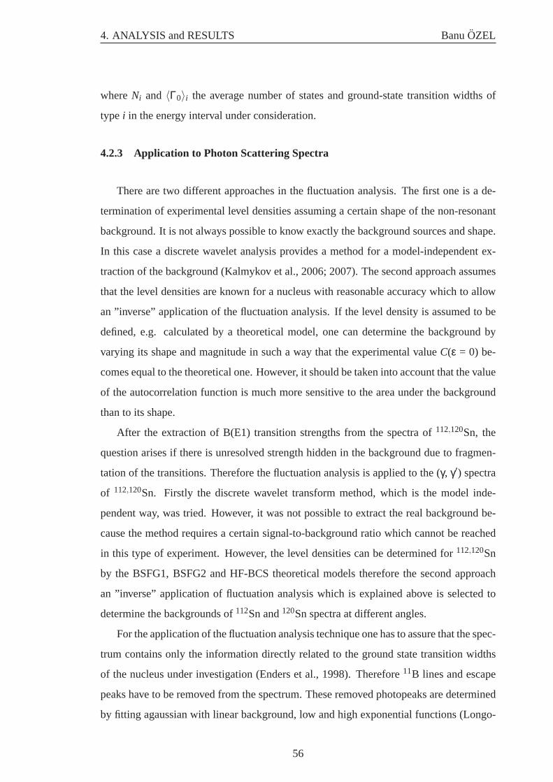
4. ANALYSIS and RESULTS BanuOZEL
whereNi and 〈Γ0〉i the average number of states and ground-state transition widths of
type i in the energy interval under consideration.
4.2.3 Application to Photon Scattering Spectra
There are two different approaches in the fluctuation analysis. The first one is a de-
termination of experimental level densities assuming a certain shape of the non-resonant
background. It is not always possible to know exactly the background sources and shape.
In this case a discrete wavelet analysis provides a method for a model-independent ex-
traction of the background (Kalmykov et al., 2006; 2007). The second approach assumes
that the level densities are known for a nucleus with reasonable accuracy which to allow
an ”inverse” application of the fluctuation analysis. If the level density is assumed to be
defined, e.g. calculated by a theoretical model, one can determine the background by
varying its shape and magnitude in such a way that the experimental valueC(ε = 0) be-
comes equal to the theoretical one. However, it should be taken into account that the value
of the autocorrelation function is much more sensitive to the area under the background
than to its shape.
After the extraction of B(E1) transition strengths from the spectra of112,120Sn, the
question arises if there is unresolved strength hidden in the background due to fragmen-
tation of the transitions. Therefore the fluctuation analysis is applied to the (γ,γ′) spectra
of 112,120Sn. Firstly the discrete wavelet transform method, which is the model inde-
pendent way, was tried. However, it was not possible to extract the real background be-
cause the method requires a certain signal-to-background ratio which cannot be reached
in this type of experiment. However, the level densities can be determined for112,120Sn
by the BSFG1, BSFG2 and HF-BCS theoretical models therefore the second approach
an ”inverse” application of fluctuation analysis which is explained above is selected to
determine the backgrounds of112Sn and120Sn spectra at different angles.
For the application of the fluctuation analysis technique one has to assure that the spec-
trum contains only the information directly related to the ground state transition widths
of the nucleus under investigation (Enders et al., 1998). Therefore11B lines and escape
peaks have to be removed from the spectrum. These removed photopeaks are determined
by fitting agaussian with linear background, low and high exponential functions (Longo-
56
4. ANALYSIS and RESULTS BanuOZEL
3 4 5 6 7 8 9 10
10-4
10-3
10-2
10-1
1
112Sn
BSFG1BSFG2HF-BCS
Energy (MeV)
<D
>(M
eV
)
Figure 4.13 Calculated level spacing,<D> for 112Sn from models of BSFG1, BSFG2 andHF-BCS. The dashed lines indicate the interval of application the fluctuation analysis.
3 4 5 6 7 8 9 10
120Sn
BSFG1BSFG2HF-BCS
Energy (MeV)
10-4
10-3
10-2
10-1
1
<D
>(M
eV
)
Figure 4.14 Calculated level spacing,<D> for 120Sn from models of BSFG1, BSFG2 andHF-BCS. The dashed lines indicate the interval of application the fluctuation analysis.
57
4. ANALYSIS and RESULTS BanuOZEL
ria, 1990) and are subtracted from spectra.
As pointed out before, the analysis is restricted to the energy region where the mean
level spacing is smaller than the experimental energy resolution. This necessary condition
is fulfilled for 112,120Sn spectra approximately above 5.5 MeV where also E1 transitions
start to increase in numbers. The level spacings are calculated from three different theo-
retical models BSFG1, BSFG2 and HF-BCS which can be seen in Fig. 4.13 for112Sn and
in Fig. 4.14 for120Sn.
Considering an inverse application of the fluctuation analysis, the region is divided in
200 keV intervals, where the background is assumed to be constant. These intervals are
individually fitted and then a smooth curve is drawn through the points defined by the
center of the intervals and the result curves are shown in Figs. 4.15 - 4.18. This process
is applied on the spectra at 90◦ and 130◦ for both isotope. The analysis is performed in
an energy region of 5.5 to 7.8 MeV. At higher energies the extraction of experimental
level densities are no longer reliable because of an overlapping in the widths and a lack
of statistics. The final backgrounds are plotted for112Sn in Fig. 4.15, Fig. 4.16 and for
120Sn in Fig. 4.17, Fig. 4.18 at 90◦ and 130◦ respectively. In these figures red lines, blue
lines and green lines correspond to the determined backgrounds assuming the NLD from
the BSFG1, BSFG2 and HF-BCS models, respectively. Although the three backgrounds
from the models are calculated independently, they show almost the same results. To
determine the strength from the spectrum, the area above the background is integrated
as B(E1) transition strength. In order to calculate the total strength for one NLD model,
an average is taken over results from 90◦ and 130◦. Extracted strengths from different
angles have similar amounts. The consistency of the results at 90◦ and 130◦ is also very
important proof to show the reliability of this analysis method. In this case three different
total strengths from the BSFG1, BSFG2 and HF-BCS have been extracted for one isotope.
For the final result an average is taken over these results.
In the integrated region SE peaks should be taken to be account. The contribution of
SE peaks is estimated by a GEANT4 simulation (Hasper, private com.) which calculates
the escapes from germanium detectors used in the present experiments. The results for
the ratio of SE to photopeak with BGO and a fit function are displayed in Fig. 4.19 in
58
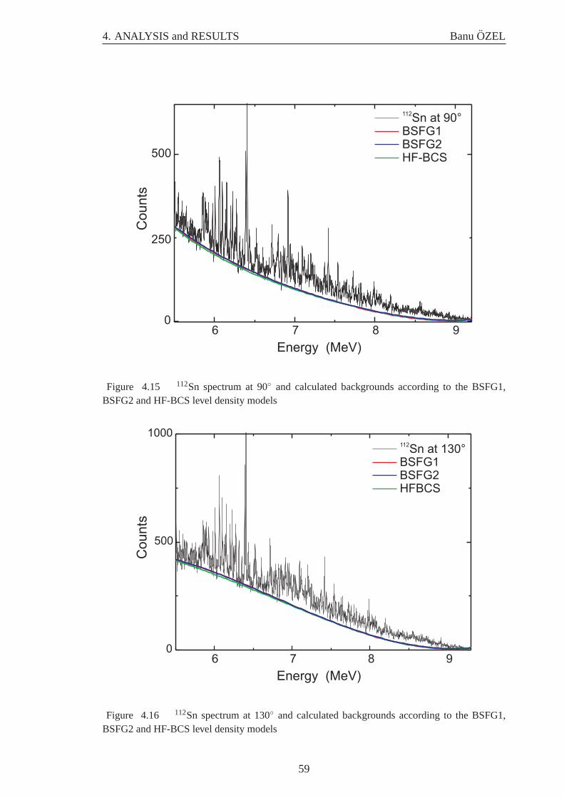
4. ANALYSIS and RESULTS BanuOZEL
6 7 8 90
500
Sn at 90°112
BSFG1BSFG2HF-BCS
Energy (MeV)
250
Co
un
ts
Figure 4.15 112Sn spectrum at 90◦ and calculated backgrounds according to the BSFG1,BSFG2 and HF-BCS level density models
0
500
1000
Sn at 130°112
BSFG1BSFG2HFBCS
6 7 8 9
Energy (MeV)
Counts
Figure 4.16 112Sn spectrum at 130◦ and calculated backgrounds according to the BSFG1,BSFG2 and HF-BCS level density models
59
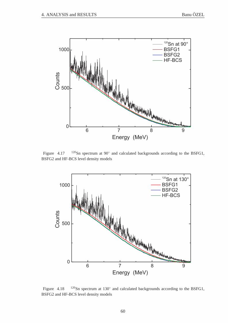
4. ANALYSIS and RESULTS BanuOZEL
0
500
1000Sn at 90°
120
BSFG1BSFG2HF-BCS
6 7 8 9
Energy (MeV)
Co
un
ts
Figure 4.17 120Sn spectrum at 90◦ and calculated backgrounds according to the BSFG1,BSFG2 and HF-BCS level density models
0
500
1000
Sn at 130°120
BSFG1BSFG2HF-BCS
6 7 8 9
Energy (MeV)
Co
un
ts
Figure 4.18 120Sn spectrum at 130◦ and calculated backgrounds according to the BSFG1,BSFG2 and HF-BCS level density models
60
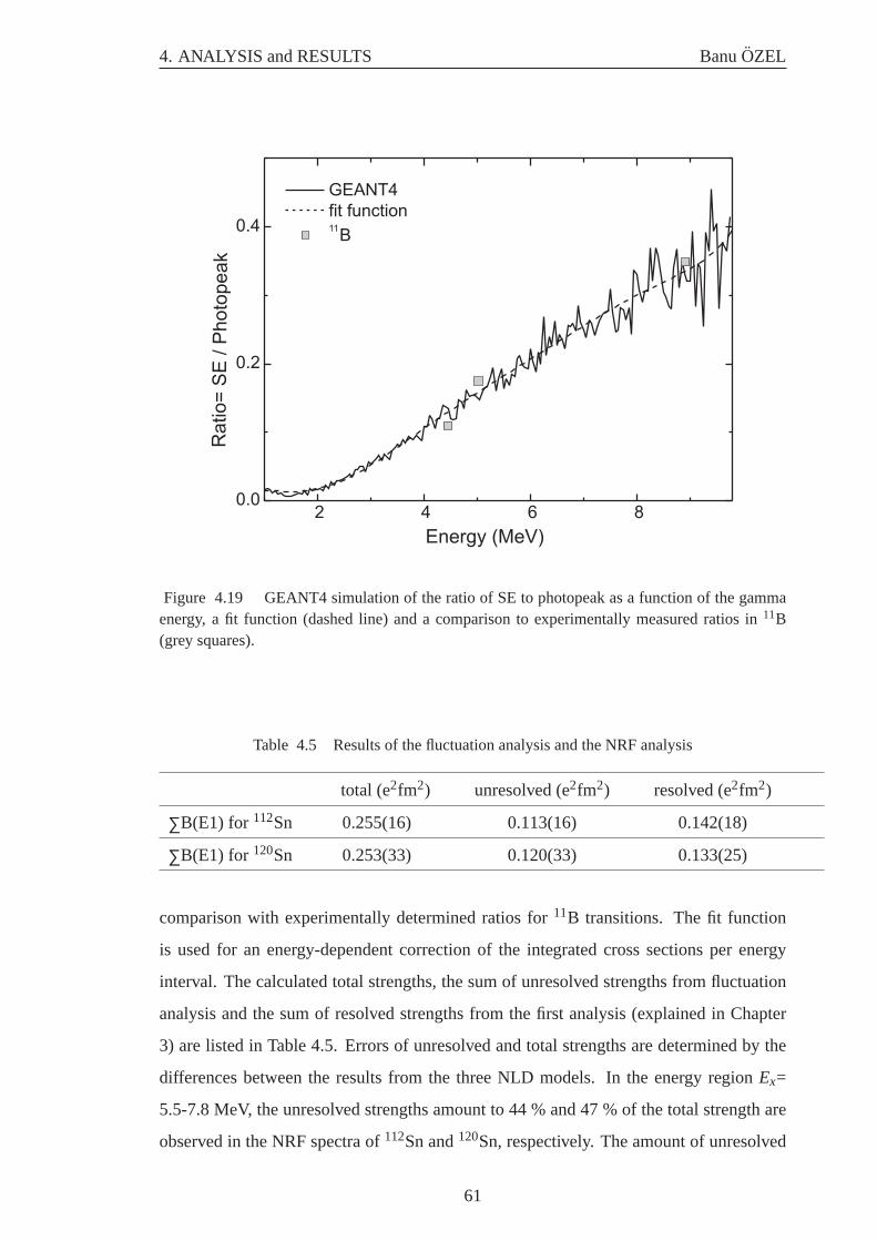
4. ANALYSIS and RESULTS BanuOZEL
0.0
0.2
0.4
GEANT4
fit function11
BR
atio=
SE
/ P
hoto
peak
2 4 6 8
Energy (MeV)
Figure 4.19 GEANT4 simulation of the ratio of SE to photopeak as a function of the gammaenergy, a fit function (dashed line) and a comparison to experimentally measured ratios in11B(grey squares).
Table 4.5 Results of the fluctuation analysis and the NRF analysis
total (e2fm2) unresolved (e2fm2) resolved (e2fm2)
∑B(E1) for 112Sn 0.255(16) 0.113(16) 0.142(18)
∑B(E1) for 120Sn 0.253(33) 0.120(33) 0.133(25)
comparison with experimentally determined ratios for11B transitions. The fit function
is used for an energy-dependent correction of the integrated cross sections per energy
interval. The calculated total strengths, the sum of unresolved strengths from fluctuation
analysis and the sum of resolved strengths from the first analysis (explained in Chapter
3) are listed in Table 4.5. Errors of unresolved and total strengths are determined by the
differences between the results from the three NLD models. In the energy regionEx=
5.5-7.8 MeV, the unresolved strengths amount to 44 % and 47 % of the total strength are
observed in the NRF spectra of112Sn and120Sn, respectively. The amount of unresolved
61

4. ANALYSIS and RESULTS BanuOZEL
strengths are very similar because, as seen from Fig. 4.13 andFig. 4.14 the level spacings
of 112Sn and120Sn show similar value with energy.
62
5. DISCUSSION and CONCLUSION BanuOZEL
5. DISCUSSION and CONCLUSION
5.1 Comparison with Theoretical Models
5.1.1 Quasiparticle Phonon Model (QPM)
The measured B(E1) transition strengths below the neutron threshold in stable tin iso-
topes are compared with theoretical models in this section. In particular, the QPM and R
QRPA are used for the comparison. The tin isotopic chain has been studied systematically
in both approaches.
The present QPM model approach is described in (Tsoneva et al., 2004a; 2004b;
2007). The model Hamiltonian is written as
H = HMF +H phM +H ph
SM+H ppM (5.1)
Here,HMF=Hsp+Hpair is the mean field part consisting of a single-particle (Hsp) and a
pairing (Hpair) part which has to be identified with the Hartree-Fock Bogoliubov (HFB)
Hamiltonian. The calculation uses single-particle energies, wave functions obtained self-
consistently and a reparameterization of the HFB mean field in terms of a Woods-Saxon
potential as described in (Tsoneva at al., 2004b).
The QPM calculations in110−132Sn contain a sequence of low-lying one-phonon 1-
states at excitation energies Ex = 6 - 7.5 MeV which shows almost pure neutron structure
with proton contributions of less than 1%. The main part of the PDR comes from one-,
two- and three quasiparticle states in this type of nonrelativistic calculations. The pre-
dicted excitation energies of these states also define the energy region of the PDR. The
results for120Sn are displayed in Fig 5.1. The quantityR is an amplitude which is entering
in the definition of the multi-phonon wave function. The square of it is a probability to
have a certain one-phonon contribution to the structure of an excited state. As seen from
the figure the PDR is concentrated in the energy region 6.5 - 7.5 MeV for this isotope.
Calculations for other even tin isotopes show almost the same energy region for the PDR
(Tsoneva, et al., private com.).
The results of a calculation with 240 one-, two- and three phonon configurations
63
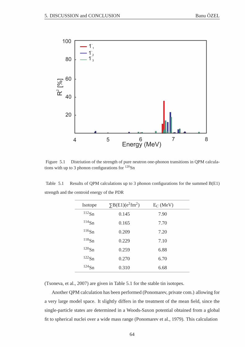
5. DISCUSSION and CONCLUSION BanuOZEL
5 7 84 6
1-
3
1-
1
1-
2
20
40
60
80R
[%]
2
Energy (MeV)
100
Figure 5.1 Distriution of the strength of pure neutron one-phonon transitions in QPM calcula-tions with up to 3 phonon configurations for120Sn
Table 5.1 Results of QPM calculations up to 3 phonon configurations for the summed B(E1)
strength and the centroid energy of the PDR
Isotope ∑B(E1)(e2fm2) EC (MeV)
112Sn 0.145 7.90
114Sn 0.165 7.70
116Sn 0.209 7.20
118Sn 0.229 7.10
120Sn 0.259 6.88
122Sn 0.270 6.70
124Sn 0.310 6.68
(Tsoneva, et al., 2007) are given in Table 5.1 for the stable tin isotopes.
Another QPM calculation has been performed (Ponomarev, private com.) allowing for
a very large model space. It slightly differs in the treatment of the mean field, since the
single-particle states are determined in a Woods-Saxon potential obtained from a global
fit to spherical nuclei over a wide mass range (Ponomarev et al., 1979). This calculation
64
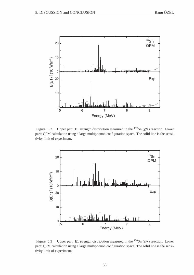
5. DISCUSSION and CONCLUSION BanuOZEL
0
10
20
0
10
20
112Sn
QPM
Exp
Energy (MeV)
5 6 7 8 9
B(E
1)
(1
0e
fm)
-32
2
Figure 5.2 Upper part: E1 strength distribution measured in the112Sn (γ,γ′) reaction. Lowerpart: QPM calculation using a large multiphonon configuration space. The solid line is the sensi-tivity limit of experiment.
5 6 7 8 9
0
10
20
0
10
20
120Sn
QPM
Energy (MeV)
B(E
1)
(1
0e
fm)
-32
2
Exp
Figure 5.3 Upper part: E1 strength distribution measured in the120Sn (γ,γ′) reaction. Lowerpart: QPM calculation using a large multiphonon configuration space. The solid line is the sensi-tivity limit of experiment.
65
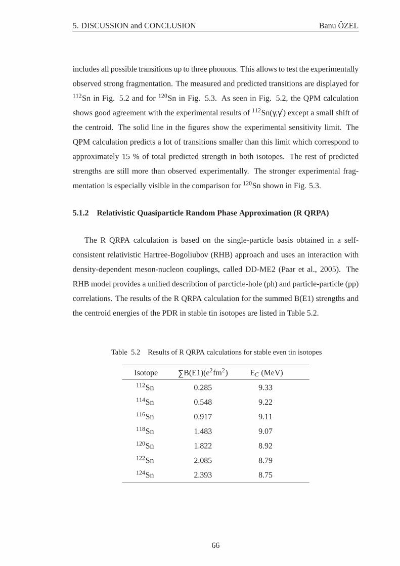
5. DISCUSSION and CONCLUSION BanuOZEL
includes all possible transitions up to three phonons. This allows to test the experimentally
observed strong fragmentation. The measured and predicted transitions are displayed for
112Sn in Fig. 5.2 and for120Sn in Fig. 5.3. As seen in Fig. 5.2, the QPM calculation
shows good agreement with the experimental results of112Sn(γ,γ′) except a small shift of
the centroid. The solid line in the figures show the experimental sensitivity limit. The
QPM calculation predicts a lot of transitions smaller than this limit which correspond to
approximately 15 % of total predicted strength in both isotopes. The rest of predicted
strengths are still more than observed experimentally. The stronger experimental frag-
mentation is especially visible in the comparison for120Sn shown in Fig. 5.3.
5.1.2 Relativistic Quasiparticle Random Phase Approximation (R QRPA)
The R QRPA calculation is based on the single-particle basis obtained in a self-
consistent relativistic Hartree-Bogoliubov (RHB) approach and uses an interaction with
density-dependent meson-nucleon couplings, called DD-ME2 (Paar et al., 2005). The
RHB model provides a unified describtion of parcticle-hole (ph) and particle-particle (pp)
correlations. The results of the R QRPA calculation for the summed B(E1) strengths and
the centroid energies of the PDR in stable tin isotopes are listed in Table 5.2.
Table 5.2 Results of R QRPA calculations for stable even tin isotopes
Isotope ∑B(E1)(e2fm2) EC (MeV)
112Sn 0.285 9.33
114Sn 0.548 9.22
116Sn 0.917 9.11
118Sn 1.483 9.07
120Sn 1.822 8.92
122Sn 2.085 8.79
124Sn 2.393 8.75
66
5. DISCUSSION and CONCLUSION BanuOZEL
5.1.3 Discussion
The experimental summed B(E1) strengths and centroid energies for112,116,120,124Sn
are compared to the theoretical QPM and R QRPA calculations (Tsoneva et al., 2007; Paar
et al., 2005) summed over an energy regionEx= 5.5-7.8 MeV in Fig 5.4. In this figure
the open triangles are R QRPA calculations, the upturned triangles are QPM calculations,
the full circles are the experimental results for112,120Sn from the analysis of discrete
transitions, the full squares are total strengths of112,120Sn which consists of measured
B(E1) strength and unresolved strength from the fluctuation analysis and the stars are the
sum of measured B(E1) strengths of116,124Sn (Govaert, et al., 1997).
The upper part of the Fig. 5.4 shows the comparison of centroid energies as a func-
tion of mass number. The results of the R QRPA calculation are much higher than the
experimental results and the QPM values. Both models predict that the centroid energies
decreases with the number of neutrons. Although the experimental results are closer to the
QPM calculation, they do not exhibit such a smooth dependence on the neutron number.
On the contrary, the experimental results show almost constant values in every isotope.
Including the unresolved strength has little effect on the centroid energies.
The lower part of Fig. 5.4 displays the sum of B(E1) transition strengths as a function
of mass number in two different scales because R QRPA predicts much higher strengths
compared to the results of experiments and QPM calculations. The R QRPA calculations
do not show agreement with experimental results except the corrected total strength of
112Sn. There is another R QRPA calculation is not shown in Fig. 5.4, but predicts almost
the same amount of E1 strength in tin isotopes (Piekarewicz, 2006) with that from Paar
(Paar et al., 2005). The much larger strength and higher centroid energy in these calcu-
lations indicate that the effective mass used in this model, which scale the single-particle
spectrum, are not correct.
Both theoretical calculations (QPM and R QRPA) predict that the sum of B(E1)
strengths should increase with the number of neutrons. The QPM calculations are
relatively close the experimental results. Without unresolved strength correction the
112,116,124Sn isotopes show good agreement with QPM predictions but120Sn would be
too small. After the correction, the sum of strengths of112Sn and120Sn are increasing by
almost 50 %. Now,120Sn is in good agreement but112Sn would be underpredicted by the
67
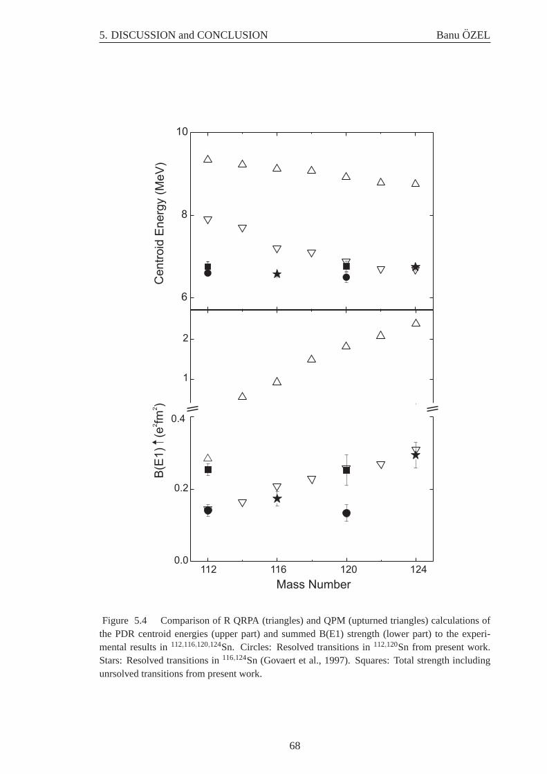
5. DISCUSSION and CONCLUSION BanuOZEL
112 116 120 124
Mass Number
6
8
10
1
2
0.0
0.2
0.4
B(E
1)
(e
fm)
22
Centr
oid
Energ
y (
MeV
)
Figure 5.4 Comparison of R QRPA (triangles) and QPM (upturned triangles) calculations ofthe PDR centroid energies (upper part) and summed B(E1) strength (lower part) to the experi-mental results in112,116,120,124Sn. Circles: Resolved transitions in112,120Sn from present work.Stars: Resolved transitions in116,124Sn (Govaert et al., 1997). Squares: Total strength includingunrsolved transitions from present work.
68
5. DISCUSSION and CONCLUSION BanuOZEL
QPM. For a realistic comparison one should also know the unresolved strength of
116,124Sn isotopes. As mentioned before in the fluctuation analysis method the selection
of background in (γ,γ′) spectrum depends on the mean level spacing of nucleus under
consideration. In this case the amount of unresolved strengths of116,124Sn isotopes can
be expected to be similar to that of112,120Sn. In such a case, the total strength of120Sn
would still be lower than other experimental corrected values. Thus, the present work
indicates that the PDR does not depend directly on the neutron excess.
However, there is an experimental problem since the present measurements are not
sensitive over the full energy region where the PDR is predicted, and omitted inelastic
branchings might become important at higher energies. On the other hand the QPM re-
sults support that the PDR is confirmed to the energy region, where strength is observed
in the (γ,γ′) For a final conclusion one needs a consistent set of data of the E1 response
from low to high energies as a real test of the models.
5.2 Conclusion and Outlook
In summary, the thesis presents high-resolution nuclear resonance fluorescence exper-
iments on112Sn and120Sn stable isotopes to investigate the E1 response below the neutron
threshold. The strongest transitions have been observed around the energy region of 6-7
MeV and the distributions of extracted B(E1) transitions have a resonance-like structure,
but in the case of120Sn the dipole strengths are more fragmented. The sum of B(E1)
strengths are 187 (24) e2fm2 and 164 (29) e2fm2 with centroid energies 6.7 MeV and 6.6
MeV for 112Sn and120Sn, respectively.
A fluctuation analysis was applied to the (γ,γ′) spectra to estimate the unresolved
strength which might be hidden in the background due to the finite energy resolution. This
analysis have been performed with the help of an autocorrelation function which provides
the information about the mean level spacing in the defined energy intervals. These can be
compared to model prediction of the NLD, which allows to adjust the background. Three
different theoretical models explained in Chapter 4 have been used: BSFG1, BSFG2
and HF-BSC (Egidy et al., 2005; Rauscher, et al., 1997; Demetriou et al., 2001). The
backgrounds determined from these models produce a very similar amount of unresolved
strength in the spectra and the differences between the models have been used to deter-
69
5. DISCUSSION and CONCLUSION BanuOZEL
mine the uncertainties of this procedure. The fluctuation analysis shows that the amount
of unresolved strength on (γ,γ′) spectra is obviously not negligible and should be applied
to other data which are taken with the NRF method, i.e. the spectra of116Sn and124Sn.
Together with the so determined unresolved part, the measured B(E1) strength distribu-
tions below the neutron threshold in112Sn and120Sn was compared to microscopic model
to understand their nature. QPM calculations with a very large multiphonon configura-
tion (Ponamarev, private com.) reasonably reproduce the fragmentation of the transition
strengths for112Sn and120Sn. The QPM and the R QRPA calculations predict a smooth
increase of the summed B(E1) strength and a decrease of the centroid energy with neutron
number in stable tin isotopes. However, the experimental results do not show a simple de-
pendence on neutron excess. This indicates that the low-energy E1 strength retains much
of its single-particle character rather than developing into a true collective mode. This is
in agreement with the picture deduced from the QPM results but contradicts the R QRPA
results.
For an improved understanding measurements of the complete E1 response below
and above the neutron threshold would be important. This is possible with high reso-
lution (p,p′) experiment at 0◦ at RCNP Osaka university (Tamii et al., 2007) and also
in near future in photon scattering experiments with new NEPTUN tagger facility at the
S-DALINAC (Lindenberg, 2007).
70
REFERENCES
AAB V. et al., Proc. 3rd Workshop on Rf Supercond., Ed. K.W.Shepard, ANL-Phy-88-1
(1988) 127.
ADAMS, J. P. et al., Phys. Rev. C 53 (1996) 1016
ADRICH, P. et al., Phys. Rev. Lett. 95 (2005) 1325
———————, Dissertation, Jagiellonian University, 2005
AUDI, G., WAPSTRA, A. H.and THIBAULT, C., Nucl. Phys. A 729, 337 (2003)
AUERHAMMER, J. et al., Nucl. Phys. A553 (1993) 841c
AUERHAMMER, J. et al., Proc. 5thWorkshop on Rf Supercond., Ed. D.Proch, DESY
M-92-01 (1992) 110
AUMANN, T., Eur. Phys. J. A 26 (2005) 441
BALBUTSEV, E. B. et al., Europhys. Lett. 26 (1994) 499
BALDWIN, G. C., KLEIBER, G. S., Phys. Rev. 71 (1947) 3
BARTHOLOMEV, G. A. et al., Adv. Nucl. Phys. 7 (1972) 229.
BASTRUKOV, S. I. et al., Nucl. Phys. A562 (1993) 191
BAUWENS, F. et al., Phys. Rev. C 62 (2000) 024302
BEAUSANG, C. W. and SIMPSON J., J. Phys. G: Nucl. Part. Phys. 22 (1996) 527
BERG U. E. P. et al., Phys. Lett. B 103 (1981) 301
BERMAN, B. L., FULTZ, S. C., Rev. Mod. Phys. 47 (1975) 713
BETHE, H. A. and PLACZEC, G., Phys. Rev 51 (1937) 450
BOHR, A. and MOTTELSON, B.R. Nuclear Structure, Vol.2, Nuclear Deformations,
W.A.Benjamin, Advanced Book Program, Massachusetts, (1975)
BOTHE, W., GENTNER, W., Z. Phys. 71 (1937) 236
BROWN, G.E. and BOLSTERLI, M., Phys. Rev. Lett. 3 (1959) 472
BRYSSINCK, J. et al., Phys. Rev. C 59 (1999) 1930
CHAMBERS, J. et al., Phys. Rev. C 50 (1994) R2671
CHAPURAN, T. , VODHANEL, R., BRUSSEL, M. K., Phys. Rev. C 22 (1980) 1420
COLO, G. et al., Phys. Lett. B 485 (2000) 362
DEMETRIOU, P. and GORIELY, S., Nucl. Phys. A 695 (2001) 95
DIETRICH, S. S., BERMAN., B. L., At. Data Nucl. Data Tables 38 (1988) 199
ENDERS, J. et al., Nucl. Phys. A 636 (1998) 139
———————–, Nucl. Phys. A 724 (2003) 243
———————–, Phys. Lett. B 486 (2000) 279
71
———————–, Phys. Rev. C 57 (1998) 996
———————–, Phys. Rev, Lett. 79 (1997) 2010
ERICSON, T., Adv. Phys. 9 (1960) 425
FUKUNISHI, N. , OTSUKA, T. , TANIHATA, I., Phys. Rev. C 48 (1993) 1648
GEIGER, W. et. al., Nucl. Phys. A 580 (1994) 263
GILBERT, A. and CAMERON, A. G., Can. J. Phys. 43 (1965) 1446
GOLDHABER, M., TELLER, E., Phys. Rev. 74 (1948) 1046
GORIELY, S., TONDEUR, F. and AERSON, J.M., At. Data Nucl. Data Tables 77 (2001)
311
GOVAERT, K. et al., Phys. Rev. C 57 (1997) 2229
GRINBERG, M. and STOYANOV, C., Nuclear Phys. A 573 (1994) 231
GUHR, T., MUELLER-GROELING and A., WEIDENMUELLER, H.A., Phys. Rep. 299
(1998)189
HANSEN, P. G., Annu. Rev. Nucl. Part. Sci. 29, 69 (1979)
HARAKEH, M. N. and van der WOUDE, A., Giant Resonances, Oxford Studies in Nu-
clear Physics, Vol. 24 (Oxford University Press, 2001)
HARTMANN, T. et al., Phys. Rev. Lett. 85 (2000) 274
HASPER, J., private communication (2007)
HERZBERG, R. D. et al., Phys. Rev. C 60 (1999) 051307(R)
HUXEL, N., et al., Nucl. Phys. A 645 (1999) 239
———————, dissertation TH Darmstadt (1997)
IACHELLO, F., Phys. Lett. 160B (1985) 1
IGNATYUK, A.V., ISREKOV, K. K. and SMIRKENKIN, Sov. J. Nucl. Phys. 29 (1979)
450
IGNATYUK, A.V., SMIRKENKIN, G.N. and TISHIN, A. S., Sov. J. Nucl. Phys. 21
(1975) 255
ILJINIV, A. S. et al., Nucl. Phys. A543 (1979) 450
HASPER, J., private communication
JONSON, B. et al., Proceedings of the 3rd International Conference on Nuclei far from
Stability, Cargese, 1976, CERN Report No. 76-13 (1976) p. 277.
KUBLER, L. et al., Phys. Rev. C 70 (2004) 064307
KALMYKOV, Y. et al., Phys. Rev. Lett. 96 (2006) 012502
—————————, Phys. Rev. Lett. 99 (2007) 202502
72
KILGUS, G. et al., Z. Phys. A 326 (1987) 41
KLIMKIEWICZ, A. et al., Phys. Rev. C 76 (2007) 051603(R)
KNEISSL, U., PITZ, H. H. and ZILGES, A., Prog. Part. Nucl. Phys. 37 (1996) 349
KNEISSL, U., PIETRALLA, N. and ZILGES, A., J. Phys. G: Nucl. Part. Phys. 32
(2006) R217
KRASZNAHORKOY, A. et al., Phys. Rev. Lett. 66 (1991) 1287
LINDENBERG, K., Dissertation, TU Darmstadt (2007)
LIPAS, P. O., Nucl. Phys. 82 (1966) 91
LONGORIA, L. C. et al., Nucl. Inst. Meth. Phys. Res. A 229 (1990) 308
METZGER, F. R., FRISCH, O. R., Progress in Nuclear Physics, London, Vol. 7, (1959)
MIGDAL, A., J. Phys. (USSR) 8 (1944) 331
MISICU, S. and S. I. BASTRUKOV, Eur. Phys. J. A 13 (2002) 399
MOHAN, R. et al., Phys. Rev. C 3 (1971) 1740
MOHR, P. et al., Nucl. Inst. Meth. Phys. Res. A 423 (1999) 480
MOLLER, P. et al., At. Data Nucl. Data Tables 59 (1995) 185
MULLER, S. et al., Phys. Lett. 113B (1982) 362
MYERS, W. D., SWIATECKI, W. J. and Wang, C. S., Nucl. Phys. A436 (1985) 185
NNDC, http://www.nndc.bnl.gov/ (2007)
OROS, A. M. et al., Phys. Rev. C 57 (1998) 990
PAAR, N. et al., Phys. Lett. B 606 (2005) 288
——————–, Phys. Rev. C 67 (2003) 034312
PIEKAREWICZ, J., Phys. Rev. C 73 (2006) 044325
PIETRALLA, N. et al., Phys. Rev. Lett. 88 (2002) 012502
PONOMAREV, V.Yu. et al., Nucl. Phys. A 323 (1979) 446
——————————, private communication
PORTER, C. E. and THOMAS, R. G., Phys. Rev. 104 (1956) 483
PYSMENETSKA, I. et al., Phys. Rev. C 73 (2006) 17302
RAUSCHER, T., THIELEMANN, F.-K. and KRATZ, K.,-L., Phys. Rav. C 56 (1997)
1613
RICHTER, A., Proceeding of the Fifth European Particle Accelerator Conference, ed. S.
Meyers et al., (IOP Publishing, Bristol, 1996) 110.
——————, Nucl. Phys. A 522 (1991) 139c.
RYEZAYEVA, N. et al., Phys. Rev. Lett. 89 (2002) 272502
73
STEINWEDEL, H. and JENSEN J. H. D., Phys. Rev. 74 (1950) 1019
SUZUKI, Y. et al., Prog. Theor. Phys. 83 (1990) 180
SCHWENGNER, R. et al., Phys. Rev. C 76 (2007) 034321
—————————, Nucl. Phys. A 788 (2007) 331c
TAMII, A. et al., Nucl.Phys. A 788, 53 (2007)
TERASAKI, J. et al., Phys. Rev. C 71 (2005) 034310
TONDEUR, F. et al., Phys. Rev. C 62 (2000) 024308
TSONEVA, N., LENSKE, H., STOYANOV, Ch., Nucl. Phys. A 731 (2004)a 273
——————, Nucl. Phys. A 586 (2004)b 213
TSONEVA, N. and LENSKE, H., arXiv:0706.4204v1 [nucl-th] 28 Jun 2007
Van ISACKER, P. et al., Phys. Rev. C 45 (1992) R13
VOGEL, P. and KOCHBACH, L., Nucl. Phys. A 176 (1971) 33
VOLZ, S. et al., Nucl. Phys. A 779 (2006) 1
——————, private communication
von EGIDY, T. and BUCURESCU, D., Phys. Rev. C 72, 044311(2005)
VRETENAR, D. et al., Phys. Rev. Lett. 91 (2003) 262502
—————————, Phys. Rev. C 65 (2002) 021301
—————————, Phys. Lett. B 487 (2000) 334
WIGNER, E. P., in: C. E. Porter (Ed.), Statistical Theories of Spectra: Fluctuations (Aca-
demic Press, New York, 1965) 200.
WONG, S. S. M., Introductory Nuclear Physics (Prentice-Hall International, Inc. 1990)
ZHONGFU, H. et al., Chin. J. Nucl. Phys. 13 (1941) 147
ZILGES, A. et al., Phys. Lett. B 542 (2002) 43
74
CURRICULUM VITAE
Name : BanuOzel
Date of Birth : 25.08.1976
Nationality : Turkish
EDUCATIONAL BACKGROUND
1994-1998 : B.Sc Ankara University
2000-2003 : M.Sc Cukurova University
2003-2008 : Ph.D Cukurova University
PROFFESSIONAL BACKGROUND
Mar. 1999 - Nov. 2000 : research assistant at Nigde University
Nov. 2000 - now : research assistant at Cukurova University
Oct.2004 - July 2005 : guest student in Institut fur Kernphysik
TU-Darmstadt, Germany with Erasmus Program
Aug. 2005 - Oct. 2007 : guest student in Institut fur Kernphysik
TU-Darmstadt, Germany with DAAD Scholarship
75