Jameson-Schmidt-Turkel (JST) scheme

Praveen. Cpraveen@math.tifrbng.res.in

Tata Institute of Fundamental ResearchCenter for Applicable Mathematics

Bangalore 560065http://math.tifrbng.res.in/~praveen

March 20, 2013

1 / 19

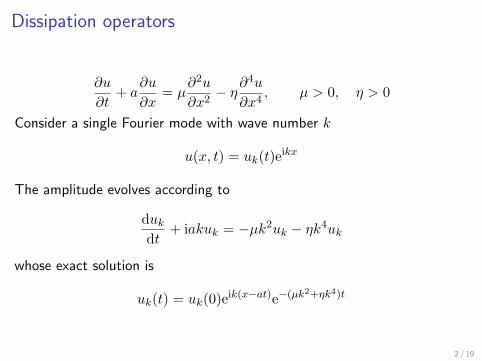
Dissipation operators

∂u

∂t+ a

∂u

∂x= µ

∂2u

∂x2− η∂

4u

∂x4, µ > 0, η > 0

Consider a single Fourier mode with wave number k

u(x, t) = uk(t)eikx

The amplitude evolves according to

dukdt

+ iakuk = −µk2uk − ηk4uk

whose exact solution is

uk(t) = uk(0)eik(x−at)e−(µk2+ηk4)t

2 / 19

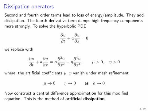
Dissipation operators

Second and fourth order terms lead to loss of energy/amplitude. They adddissipation. The fourth derivative term damps high frequency componentsmore strongly. To solve the hyperbolic PDE

∂u

∂t+ a

∂u

∂x= 0

we replace with

∂u

∂t+ a

∂u

∂x= µ

∂2u

∂x2− η∂

4u

∂x4, µ > 0, η > 0

where, the artificial coefficients µ, η vanish under mesh refinement

µ→ 0 η → 0 as h→ 0

Now construct a central difference approximation for this modifiedequation. This is the method of artificial dissipation.

3 / 19

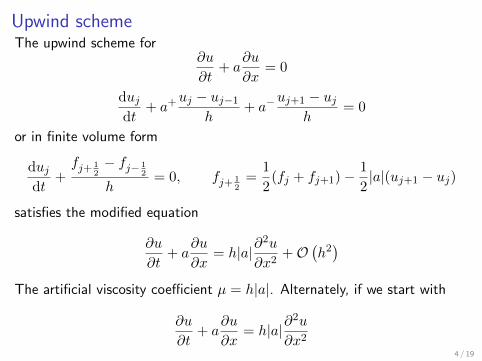
Upwind schemeThe upwind scheme for

∂u

∂t+ a

∂u

∂x= 0

dujdt

+ a+uj − uj−1

h+ a−

uj+1 − ujh

= 0

or in finite volume form

dujdt

+fj+ 1

2− fj− 1

2

h= 0, fj+ 1

2=

1

2(fj + fj+1)−

1

2|a|(uj+1 − uj)

satisfies the modified equation

∂u

∂t+ a

∂u

∂x= h|a|∂

2u

∂x2+O

(h2)

The artificial viscosity coefficient µ = h|a|. Alternately, if we start with

∂u

∂t+ a

∂u

∂x= h|a|∂

2u

∂x24 / 19

Upwind scheme

and discretize with central differences

dujdt

+ auj+1 − uj+1

2h= h|a|uj−1 − 2uj + uj+1

h2

then we obtain the upwind scheme.

5 / 19

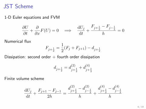
JST Scheme

1-D Euler equations and FVM

∂U

∂t+

∂

∂xF (U) = 0 =⇒ dUj

dt+Fj+ 1

2− Fj− 1

2

h= 0

Numerical flux

Fj+ 12

=1

2(Fj + Fj+1)− dj+ 1

2

Dissipation: second order + fourth order dissipation

dj+ 12

= d(2)

j+ 12

+ d(4)

j+ 12

Finite volume scheme

dUjdt

+Fj+1 − Fj−1

2h=d(2)

j+ 12

− d(2)j− 1

2

h+d(4)

j+ 12

− d(4)j− 1

2

h

6 / 19

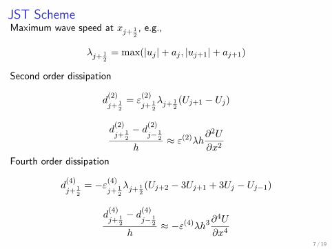
JST SchemeMaximum wave speed at xj+ 1

2, e.g.,

λj+ 12

= max(|uj |+ aj , |uj+1|+ aj+1)

Second order dissipation

d(2)

j+ 12

= ε(2)

j+ 12

λj+ 12(Uj+1 − Uj)

d(2)

j+ 12

− d(2)j− 1

2

h≈ ε(2)λh∂

2U

∂x2

Fourth order dissipation

d(4)

j+ 12

= −ε(4)j+ 1

2

λj+ 12(Uj+2 − 3Uj+1 + 3Uj − Uj−1)

d(4)

j+ 12

− d(4)j− 1

2

h≈ −ε(4)λh3∂

4U

∂x4

7 / 19

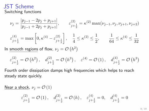
JST SchemeSwitching functions

νj =|pj−1 − 2pj + pj+1||pj−1 + 2pj + pj+1|

, ε(2)

j+ 12

= κ(2) max(νj−1, νj , νj+1, νj+2)

ε(4)

j+ 12

= max

[0, κ(4) − ε(2)

j+ 12

],

1

4≤ κ(2) ≤ 1

2,

1

64≤ κ(4) ≤ 1

32

In smooth regions of flow, νj = O(h2)

ε(2)

j+ 12

= O(h2), d

(2)

j+ 12

= O(h3), ε(4) = O (1) , d

(4)

j+ 12

= O(h3)

Fourth order dissipation damps high frequencies which helps to reachsteady state quickly.

Near a shock, νj = O (1)

ε(2)

j+ 12

= O (1) , d(2)

j+ 12

= O (h) , ε(4)

j+ 12

= 0, d(4)

j+ 12

= 0

8 / 19

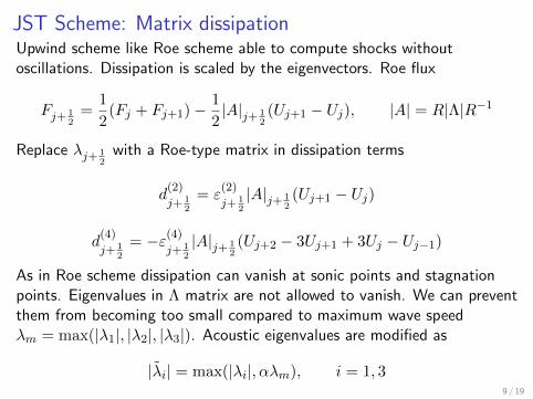
JST Scheme: Matrix dissipationUpwind scheme like Roe scheme able to compute shocks withoutoscillations. Dissipation is scaled by the eigenvectors. Roe flux

Fj+ 12

=1

2(Fj + Fj+1)−

1

2|A|j+ 1

2(Uj+1 − Uj), |A| = R|Λ|R−1

Replace λj+ 12

with a Roe-type matrix in dissipation terms

d(2)

j+ 12

= ε(2)

j+ 12

|A|j+ 12(Uj+1 − Uj)

d(4)

j+ 12

= −ε(4)j+ 1

2

|A|j+ 12(Uj+2 − 3Uj+1 + 3Uj − Uj−1)

As in Roe scheme dissipation can vanish at sonic points and stagnationpoints. Eigenvalues in Λ matrix are not allowed to vanish. We can preventthem from becoming too small compared to maximum wave speedλm = max(|λ1|, |λ2|, |λ3|). Acoustic eigenvalues are modified as

|λ̃i| = max(|λi|, αλm), i = 1, 39 / 19

JST Scheme: Matrix dissipation

and convective eigenvalue as

|λ̃2| = max(|λ2|, βλm)

Typical values

α ≈ 0.25, β ≈ 0.025

10 / 19

TVD property

The JST scheme with scalar dissipation may still produce oscillations atstrong shocks. For scalar problems, if the numerical flux is written as

Fj+ 12

=1

2(Fj + Fj+1)−

1

2Qj+ 1

2(Uj+1 − Uj)

then it is TVD provided

Qj+ 12≥ |A|j+ 1

2, A = F ′(U)

A modified switch proposed by Swanson and Turkel (1992) makes thescheme TVD for scalar problems

νj =|pj−1 − 2pj + pj+1|

|pj − pj−1|+ |pj+1 − pj |+ ε, κ(2) =

1

2

11 / 19

TVD property

This leads to too much dissipation of shocks and in practice a weaker formof the switching function is used

νj =|pj−1 − 2pj + pj+1|(1− ω)Pj + ωQj

, 0 ≤ ω ≤ 1

Pj = |pj − pj−1|+ |pj+1 − pj |, Qj = |pj−1 + 2pj + pj+1|

ω = 0 gives the TVD switch and ω = 1 gives the JST switch. Typically, avalue of ω = 1

2 can be used for problems with strong shocks.

12 / 19

SLIP scheme

JST scheme uses pressure based switch for all flow components. It forcesall variables to be treated equally though they may experience differentchanges through a discontinuity.

Jameson introduced SLIP (Symmetric limited posititive) scheme whichmakes use of limiters.

R(u, v) = 1−∣∣∣∣ u− v|u|+ |v|+ ε

∣∣∣∣q , q > 0

1 If u and v have opposite sign then R(u, v) ≈ 0.

2 If u, v are close to one another, then R(u, v) ≈ 1.

13 / 19

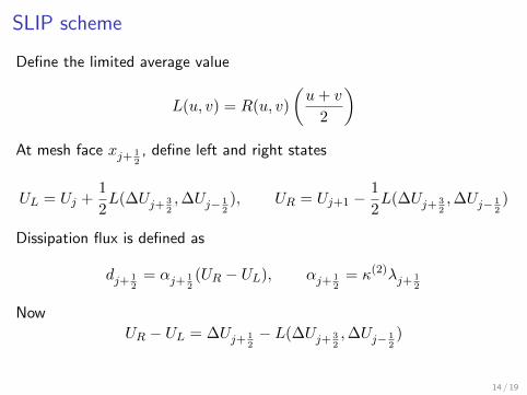
SLIP scheme

Define the limited average value

L(u, v) = R(u, v)

(u+ v

2

)At mesh face xj+ 1

2, define left and right states

UL = Uj +1

2L(∆Uj+ 3

2,∆Uj− 1

2), UR = Uj+1 −

1

2L(∆Uj+ 3

2,∆Uj− 1

2)

Dissipation flux is defined as

dj+ 12

= αj+ 12(UR − UL), αj+ 1

2= κ(2)λj+ 1

2

Now

UR − UL = ∆Uj+ 12− L(∆Uj+ 3

2,∆Uj− 1

2)

14 / 19

SLIP scheme

Near a shock, we get second order dissipation

UR − UL = ∆Uj+ 12, dj+ 1

2= αj+ 1

2(Uj+1 − Uj)

In smooth regions, we get fourth order dissipation

UR − UL ≈ ∆Uj+ 12− 1

2(∆Uj+ 3

2+ ∆Uj− 1

2)

= −1

2(Uj+2 − 3Uj+1 + 3Uj − Uj−1)

≈ −1

2h3∂3U

∂x3

15 / 19

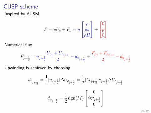
CUSP schemeInspired by AUSM

F = uUc + Fp = u

ρρuρH

+

0p0

Numerical flux

Fj+ 12

= uj+ 12

Ucj + Ucj+1

2− dc

j+12

+Fpj + Fpj+1

2− dp

j+12

Upwinding is achieved by choosing

dcj+1

2

=1

2|uj+ 1

2|∆Uc

j+12

=1

2|Mj+ 1

2|cj+ 1

2∆Uc

j+12

dpj+1

2

=1

2sign(M)

0∆pj+ 1

2

0

16 / 19

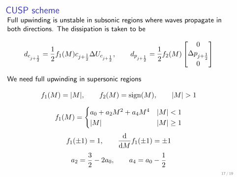
CUSP schemeFull upwinding is unstable in subsonic regions where waves propagate inboth directions. The dissipation is taken to be

dcj+1

2

=1

2f1(M)cj+ 1

2∆Uc

j+12

, dpj+1

2

=1

2f2(M)

0∆pj+ 1

2

0

We need full upwinding in supersonic regions

f1(M) = |M |, f2(M) = sign(M), |M | > 1

f1(M) =

{a0 + a2M

2 + a4M4 |M | < 1

|M | |M | ≥ 1

f1(±1) = 1,d

dMf1(±1) = ±1

a2 =3

2− 2a0, a4 = a0 −

1

217 / 19

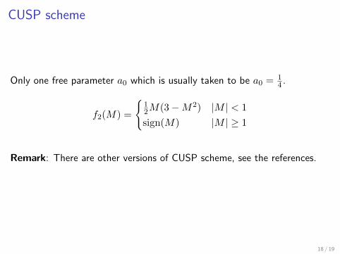
CUSP scheme

Only one free parameter a0 which is usually taken to be a0 = 14 .

f2(M) =

{12M(3−M2) |M | < 1

sign(M) |M | ≥ 1

Remark: There are other versions of CUSP scheme, see the references.

18 / 19

• A. Jameson, “Artificial diffusion, upwind biasing, limiters and theireffect on accuracy and multigrid convergence in transonic andhypersonic flows”, 11’th AIAA CFD Conference, Orlando, 1993.

• R. C. Swanson, R. Radespiel and E. Turkel, “Comparison of severaldissipation algorithms for central difference schemes”, ICASE ReportNo. 97-40, 1997.

• R. C. Swanson and E. Turkel, “On central difference and upwindschemes”, JCP, 101:292-306, 1992.

19 / 19