Finite volume method for boundary value...
38
Finite volume method for boundary value problem Discontinuous coefficients and high Peclet number Praveen. C [email protected] Tata Institute of Fundamental Research Center for Applicable Mathematics Bangalore 560065 http://math.tifrbng.res.in/ ~ praveen January 21, 2013 1 / 38
Transcript of Finite volume method for boundary value...
Finite volume method for boundary value problemDiscontinuous coefficients and high Peclet number
Praveen. [email protected]
Tata Institute of Fundamental ResearchCenter for Applicable Mathematics
Bangalore 560065http://math.tifrbng.res.in/~praveen
January 21, 2013
1 / 38
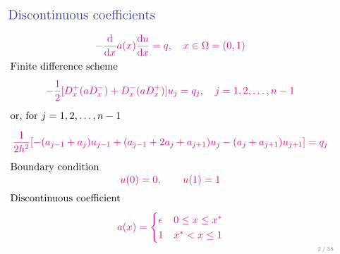
Discontinuous coefficients
− d
dxa(x)
du
dx= q, x ∈ Ω = (0, 1)
Finite difference scheme
−1
2[D+
x (aD−x ) +D−x (aD+x )]uj = qj , j = 1, 2, . . . , n− 1
or, for j = 1, 2, . . . , n− 1
1
2h2[−(aj−1 + aj)uj−1 + (aj−1 + 2aj + aj+1)uj − (aj + aj+1)uj+1] = qj
Boundary conditionu(0) = 0, u(1) = 1
Discontinuous coefficient
a(x) =
ε 0 ≤ x ≤ x∗1 x∗ < x ≤ 1
2 / 38
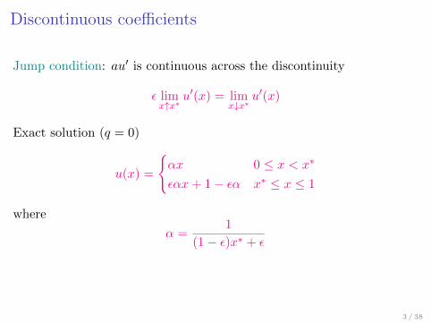
Discontinuous coefficients
Jump condition: au′ is continuous across the discontinuity
ε limx↑x∗
u′(x) = limx↓x∗
u′(x)
Exact solution (q = 0)
u(x) =
αx 0 ≤ x < x∗
εαx+ 1− εα x∗ ≤ x ≤ 1
where
α =1
(1− ε)x∗ + ε
3 / 38
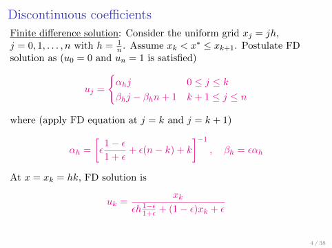
Discontinuous coefficients
Finite difference solution: Consider the uniform grid xj = jh,j = 0, 1, . . . , n with h = 1
n . Assume xk < x∗ ≤ xk+1. Postulate FDsolution as (u0 = 0 and un = 1 is satisfied)
uj =
αhj 0 ≤ j ≤ kβhj − βhn+ 1 k + 1 ≤ j ≤ n
where (apply FD equation at j = k and j = k + 1)
αh =
[ε1− ε1 + ε
+ ε(n− k) + k
]−1
, βh = εαh
At x = xk = hk, FD solution is
uk =xk
εh1−ε1+ε + (1− ε)xk + ε
4 / 38
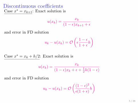
Discontinuous coefficientsCase x∗ = xk+1: Exact solution is
u(xk) =xk
(1− ε)xk+1 + ε
and error in FD solution
uk − u(xk) = O(ε1− ε1 + ε
h
)
Case x∗ = xk + h/2: Exact solution is
u(xk) =xk
(1− ε)xk + ε+ 12h(1− ε)
and error in FD solution
uk − u(xk) = O(
(1− ε)2
ε(1 + ε)h
)5 / 38
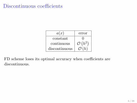
Discontinuous coefficients
a(x) error
constant 0continuous O
(h2)
discontinuous O (h)
FD scheme loses its optimal accuracy when coefficients arediscontinuous.
6 / 38
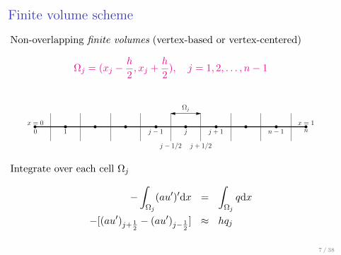
Finite volume scheme
Non-overlapping finite volumes (vertex-based or vertex-centered)
Ωj = (xj −h
2, xj +
h
2), j = 1, 2, . . . , n− 1
0 1 n− 1 njj − 1 j + 1
j − 1/2 j + 1/2
Ωj
x = 0 x = 1
Integrate over each cell Ωj
−∫
Ωj
(au′)′dx =
∫Ωj
qdx
−[(au′)j+ 12− (au′)j− 1
2] ≈ hqj
7 / 38
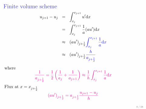
Finite volume scheme
uj+1 − uj =
∫ xj+1
xj
u′dx
=
∫ xj+1
xj
1
a(au′)dx
≈ (au′)j+ 12
∫ xj+1
xj
1
adx
≈ (au′)j+ 12
h
aj+ 12
where1
aj+ 12
=1
2
(1
aj+
1
aj+1
)≈ 1
h
∫ xj+1
xj
1
adx
Flux at x = xj+ 12
(au′)j+ 12
= aj+ 12
uj+1 − ujh
8 / 38
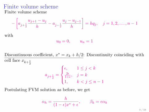
Finite volume schemeFinite volume scheme
−[aj+ 1
2
uj+1 − ujh
− aj− 12
uj − uj−1
h
]= hqj , j = 1, 2, . . . , n− 1
withu0 = 0, un = 1
Discontinuous coefficient, x∗ = xk + h/2: Discontinuity coinciding withcell face xk+ 1
2
aj+ 12
=
ε, 1 ≤ j < k2ε
1+ε , j = k
1, k < j ≤ n− 1
Postulating FVM solution as before, we get
αh =h
(1− ε)x∗ + ε, βh = εαh
9 / 38
Finite volume scheme
The FVM solution is exact !!! In general, the error of FV solution isO(h2).
Discontinuous coefficient, x∗ = xk: Discontinuity inside a cell
aj+ 12
is again given as in previous case and the error in uk is O(h2)
(show this).
When dealing with problems with discontinuous coefficients and/orsolutions, finite volume methods are more accurate than finitedifference methods. FVM has better mathematical basis since it isbased on weak formulation.
10 / 38
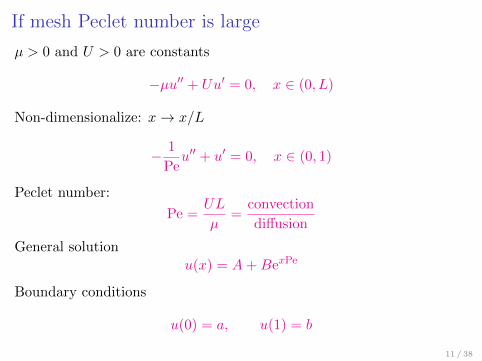
If mesh Peclet number is large
µ > 0 and U > 0 are constants
−µu′′ + Uu′ = 0, x ∈ (0, L)
Non-dimensionalize: x→ x/L
− 1
Peu′′ + u′ = 0, x ∈ (0, 1)
Peclet number:
Pe =UL
µ=
convection
diffusion
General solution
u(x) = A+BexPe
Boundary conditions
u(0) = a, u(1) = b
11 / 38
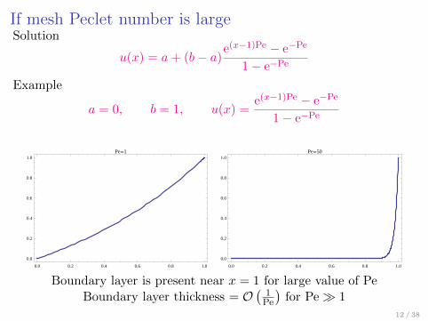
If mesh Peclet number is largeSolution
u(x) = a+ (b− a)e(x−1)Pe − e−Pe
1− e−Pe
Example
a = 0, b = 1, u(x) =e(x−1)Pe − e−Pe
1− e−Pe
0.0 0.2 0.4 0.6 0.8 1.0
0.0
0.2
0.4
0.6
0.8
1.0Pe=1
0.0 0.2 0.4 0.6 0.8 1.0
0.0
0.2
0.4
0.6
0.8
1.0Pe=50
Boundary layer is present near x = 1 for large value of PeBoundary layer thickness = O
(1
Pe
)for Pe 1
12 / 38
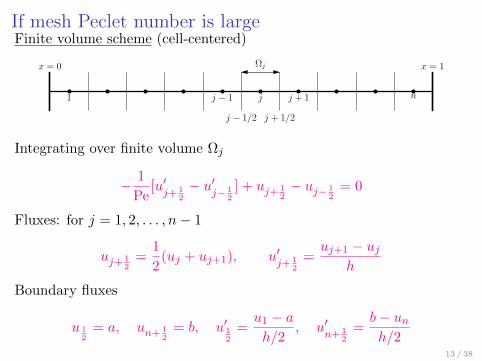
If mesh Peclet number is largeFinite volume scheme (cell-centered)
1 njj − 1 j + 1
j − 1/2 j + 1/2
Ωjx = 0 x = 1
Integrating over finite volume Ωj
− 1
Pe[u′j+ 1
2
− u′j− 1
2
] + uj+ 12− uj− 1
2= 0
Fluxes: for j = 1, 2, . . . , n− 1
uj+ 12
=1
2(uj + uj+1), u′
j+ 12
=uj+1 − uj
h
Boundary fluxes
u 12
= a, un+ 12
= b, u′12
=u1 − ah/2
, u′n+ 1
2
=b− unh/2
13 / 38
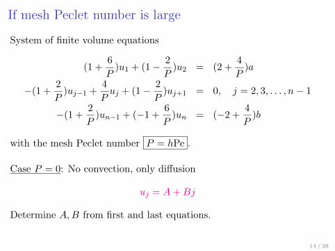
If mesh Peclet number is large
System of finite volume equations
(1 +6
P)u1 + (1− 2
P)u2 = (2 +
4
P)a
−(1 +2
P)uj−1 +
4
Puj + (1− 2
P)uj+1 = 0, j = 2, 3, . . . , n− 1
−(1 +2
P)un−1 + (−1 +
6
P)un = (−2 +
4
P)b
with the mesh Peclet number P = hPe .
Case P = 0: No convection, only diffusion
uj = A+Bj
Determine A,B from first and last equations.
14 / 38
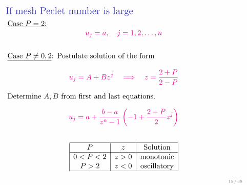
If mesh Peclet number is largeCase P = 2:
uj = a, j = 1, 2, . . . , n
Case P 6= 0, 2: Postulate solution of the form
uj = A+Bzj =⇒ z =2 + P
2− PDetermine A,B from first and last equations.
uj = a+b− azn − 1
(−1 +
2− P2
zj)
P z Solution
0 < P < 2 z > 0 monotonicP > 2 z < 0 oscillatory
15 / 38
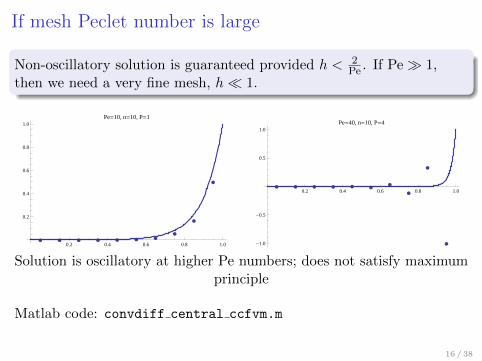
If mesh Peclet number is large
Non-oscillatory solution is guaranteed provided h < 2Pe . If Pe 1,
then we need a very fine mesh, h 1.
æ æ æ æ æ æ ææ
æ
æ
0.2 0.4 0.6 0.8 1.0
0.2
0.4
0.6
0.8
1.0Pe=10, n=10, P=1
æ æ æ æ æ ææ
æ
æ
æ
0.2 0.4 0.6 0.8 1.0
-1.0
-0.5
0.5
1.0Pe=40, n=10, P=4
Solution is oscillatory at higher Pe numbers; does not satisfy maximumprinciple
Matlab code: convdiff central ccfvm.m
16 / 38
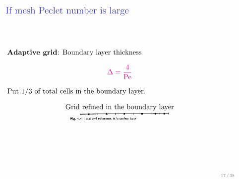
If mesh Peclet number is large
Adaptive grid: Boundary layer thickness
∆ =4
Pe
Put 1/3 of total cells in the boundary layer.
Grid refined in the boundary layer
17 / 38
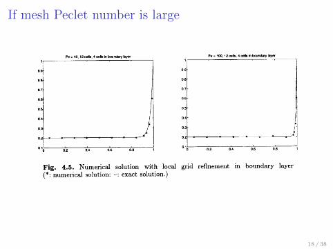
If mesh Peclet number is large
18 / 38
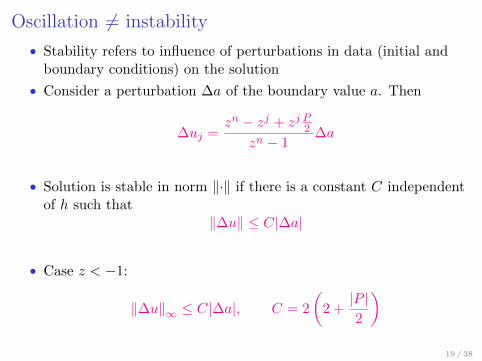
Oscillation 6= instability
• Stability refers to influence of perturbations in data (initial andboundary conditions) on the solution
• Consider a perturbation ∆a of the boundary value a. Then
∆uj =zn − zj + zj P2
zn − 1∆a
• Solution is stable in norm ‖·‖ if there is a constant C independentof h such that
‖∆u‖ ≤ C|∆a|
• Case z < −1:
‖∆u‖∞ ≤ C|∆a|, C = 2
(2 +|P |2
)19 / 38
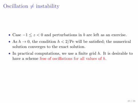
Oscillation 6= instability
• Case −1 ≤ z < 0 and perturbations in b are left as an exercise.
• As h→ 0, the condition h < 2/Pe will be satisfied; the numericalsolution converges to the exact solution.
• In practical computations, we use a finite grid h. It is desirable tohave a scheme free of oscillations for all values of h.
20 / 38
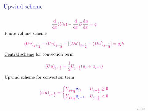
Upwind scheme
d
dx(Uu)− d
dxD
du
dx= q
Finite volume scheme
(Uu)j+ 12− (Uu)j− 1
2− [(Du′)j+ 1
2− (Du′)j− 1
2] = qjh
Central scheme for convection term
(Uu)j+ 12
=1
2Uj+ 1
2(uj + uj+1)
Upwind scheme for convection term
(Uu)j+ 12
=
Uj+ 1
2uj , Uj+ 1
2≥ 0
Uj+ 12uj+1, Uj+ 1
2< 0
21 / 38
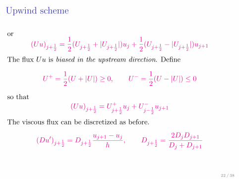
Upwind scheme
or
(Uu)j+ 12
=1
2(Uj+ 1
2+ |Uj+ 1
2|)uj +
1
2(Uj+ 1
2− |Uj+ 1
2|)uj+1
The flux Uu is biased in the upstream direction. Define
U+ =1
2(U + |U |) ≥ 0, U− =
1
2(U − |U |) ≤ 0
so that
(Uu)j+ 12
= U+j+ 1
2
uj + U−j− 1
2
uj+1
The viscous flux can be discretized as before.
(Du′)j+ 12
= Dj+ 12
uj+1 − ujh
, Dj+ 12
=2DjDj+1
Dj +Dj+1
22 / 38
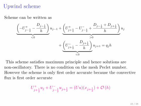
Upwind scheme
Scheme can be written as(−U+
j− 12
−Dj− 1
2
h
)︸ ︷︷ ︸
<0
uj−1 +
(U+j+ 1
2
− U−j− 1
2
+Dj− 1
2+Dj+ 1
2
h
)︸ ︷︷ ︸
>0
uj
+
(U−j+ 1
2
−Dj+ 1
2
h
)︸ ︷︷ ︸
<0
uj+1 = qjh
This scheme satisfies maximum principle and hence solutions arenon-oscillatory. There is no condition on the mesh Peclet number.However the scheme is only first order accurate because the convectiveflux is first order accurate
U+j+ 1
2
uj + U−j− 1
2
uj+ 12
= (Uu)(xj+ 12) +O (h)
23 / 38
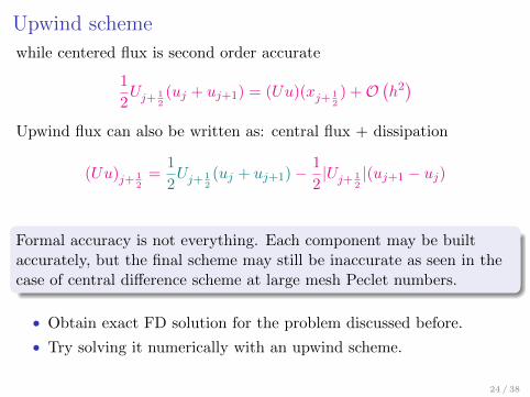
Upwind scheme
while centered flux is second order accurate
1
2Uj+ 1
2(uj + uj+1) = (Uu)(xj+ 1
2) +O
(h2)
Upwind flux can also be written as: central flux + dissipation
(Uu)j+ 12
=1
2Uj+ 1
2(uj + uj+1)− 1
2|Uj+ 1
2|(uj+1 − uj)
Formal accuracy is not everything. Each component may be builtaccurately, but the final scheme may still be inaccurate as seen in thecase of central difference scheme at large mesh Peclet numbers.
• Obtain exact FD solution for the problem discussed before.
• Try solving it numerically with an upwind scheme.
24 / 38
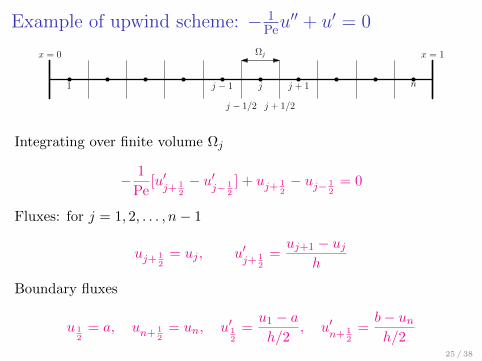
Example of upwind scheme: − 1Peu
′′ + u′ = 0
1 njj − 1 j + 1
j − 1/2 j + 1/2
Ωjx = 0 x = 1
Integrating over finite volume Ωj
− 1
Pe[u′j+ 1
2
− u′j− 1
2
] + uj+ 12− uj− 1
2= 0
Fluxes: for j = 1, 2, . . . , n− 1
uj+ 12
= uj , u′j+ 1
2
=uj+1 − uj
h
Boundary fluxes
u 12
= a, un+ 12
= un, u′12
=u1 − ah/2
, u′n+ 1
2
=b− unh/2
25 / 38
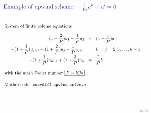
Example of upwind scheme: − 1Peu
′′ + u′ = 0
System of finite volume equations
(1 +2
P)u1 −
1
Pu2 = (1 +
1
P)a
−(1 +1
P)uj−1 + (1 +
2
P)uj −
1
Puj+1 = 0, j = 2, 3, . . . , n− 1
−(1 +1
P)un−1 + (1 +
3
P)un =
2
Pb
with the mesh Peclet number P = hPe .
Matlab code: convdiff upwind ccfvm.m
26 / 38
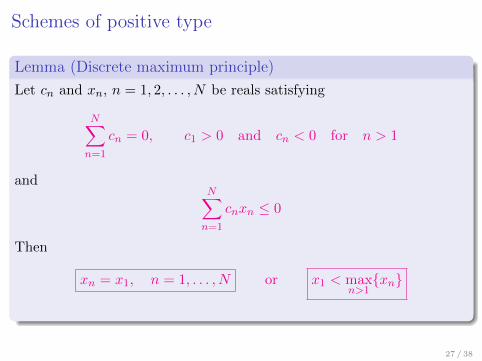
Schemes of positive type
Lemma (Discrete maximum principle)
Let cn and xn, n = 1, 2, . . . , N be reals satisfying
N∑n=1
cn = 0, c1 > 0 and cn < 0 for n > 1
andN∑n=1
cnxn ≤ 0
Then
xn = x1, n = 1, . . . , N or x1 < maxn>1xn
27 / 38
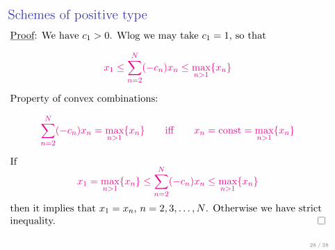
Schemes of positive type
Proof: We have c1 > 0. Wlog we may take c1 = 1, so that
x1 ≤N∑n=2
(−cn)xn ≤ maxn>1xn
Property of convex combinations:
N∑n=2
(−cn)xn = maxn>1xn iff xn = const = max
n>1xn
If
x1 = maxn>1xn ≤
N∑n=2
(−cn)xn ≤ maxn>1xn
then it implies that x1 = xn, n = 2, 3, . . . , N . Otherwise we have strictinequality.
28 / 38
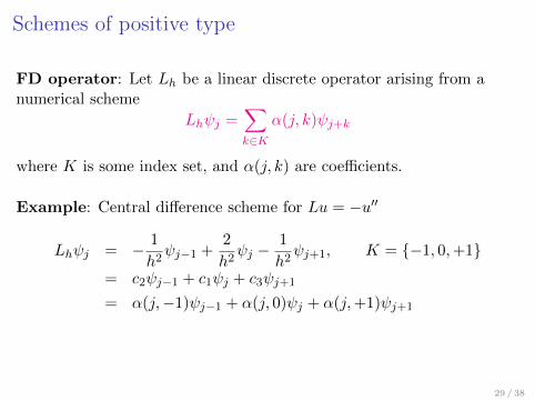
Schemes of positive type
FD operator: Let Lh be a linear discrete operator arising from anumerical scheme
Lhψj =∑k∈K
α(j, k)ψj+k
where K is some index set, and α(j, k) are coefficients.
Example: Central difference scheme for Lu = −u′′
Lhψj = − 1
h2ψj−1 +
2
h2ψj −
1
h2ψj+1, K = −1, 0,+1
= c2ψj−1 + c1ψj + c3ψj+1
= α(j,−1)ψj−1 + α(j, 0)ψj + α(j,+1)ψj+1
29 / 38
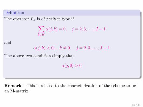
Definition
The operator Lh is of positive type if∑k∈K
α(j, k) = 0, j = 2, 3, . . . , J − 1
andα(j, k) < 0, k 6= 0, j = 2, 3, . . . , J − 1
The above two conditions imply that
α(j, 0) > 0
Remark: This is related to the characterization of the scheme to bean M-matrix.
30 / 38
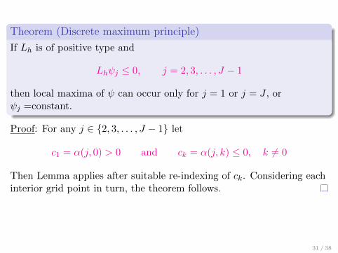
Theorem (Discrete maximum principle)
If Lh is of positive type and
Lhψj ≤ 0, j = 2, 3, . . . , J − 1
then local maxima of ψ can occur only for j = 1 or j = J , orψj =constant.
Proof: For any j ∈ 2, 3, . . . , J − 1 let
c1 = α(j, 0) > 0 and ck = α(j, k) ≤ 0, k 6= 0
Then Lemma applies after suitable re-indexing of ck. Considering eachinterior grid point in turn, the theorem follows.
31 / 38
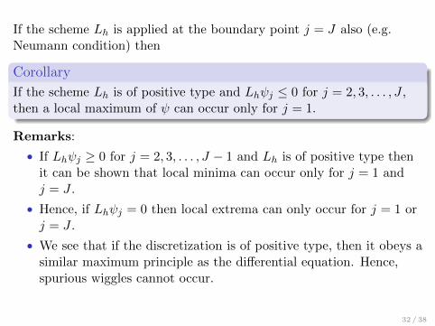
If the scheme Lh is applied at the boundary point j = J also (e.g.Neumann condition) then
Corollary
If the scheme Lh is of positive type and Lhψj ≤ 0 for j = 2, 3, . . . , J ,then a local maximum of ψ can occur only for j = 1.
Remarks:
• If Lhψj ≥ 0 for j = 2, 3, . . . , J − 1 and Lh is of positive type thenit can be shown that local minima can occur only for j = 1 andj = J .
• Hence, if Lhψj = 0 then local extrema can only occur for j = 1 orj = J .
• We see that if the discretization is of positive type, then it obeys asimilar maximum principle as the differential equation. Hence,spurious wiggles cannot occur.
32 / 38
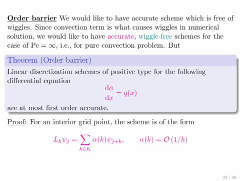
Order barrier We would like to have accurate scheme which is free ofwiggles. Since convection term is what causes wiggles in numericalsolution, we would like to have accurate, wiggle-free schemes for thecase of Pe =∞, i.e., for pure convection problem. But
Theorem (Order barrier)
Linear discretization schemes of positive type for the followingdifferential equation
dφ
dx= q(x)
are at most first order accurate.
Proof: For an interior grid point, the scheme is of the form
Lhψj =∑k∈K
α(k)ψj+k, α(k) = O (1/h)
33 / 38
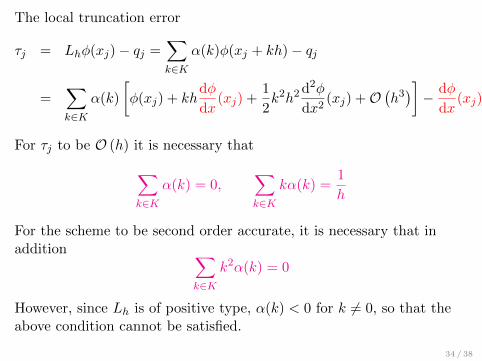
The local truncation error
τj = Lhφ(xj)− qj =∑k∈K
α(k)φ(xj + kh)− qj
=∑k∈K
α(k)
[φ(xj) + kh
dφ
dx(xj) +
1
2k2h2 d2φ
dx2(xj) +O
(h3)]− dφ
dx(xj)
For τj to be O (h) it is necessary that∑k∈K
α(k) = 0,∑k∈K
kα(k) =1
h
For the scheme to be second order accurate, it is necessary that inaddition ∑
k∈Kk2α(k) = 0
However, since Lh is of positive type, α(k) < 0 for k 6= 0, so that theabove condition cannot be satisfied.
34 / 38
Remark: A similar order barrier theorem holds for time-dependentcase. A way to get around this is to use nonlinear schemes even forlinear problems. In practice, it is preferable to use high order accurateschemes, atleast second order (τj = O
(h2)), in order to get reliable
results at small computational cost.
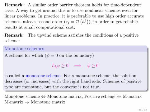
Remark: The upwind scheme satisfies the conditions of a positivescheme.
Monotone schemes
A scheme for which (ψ = 0 on the boundary)
Lhψ ≥ 0 =⇒ ψ ≥ 0
is called a monotone scheme. For a monotone scheme, the solutiondecreases (or increases) with the right hand side. Schemes of positivetype are monotone, but the converse is not true.
Monotone scheme ⇔ Monotone matrix, Positive scheme ⇔ M-matrixM-matrix ⇒ Monotone matrix
35 / 38
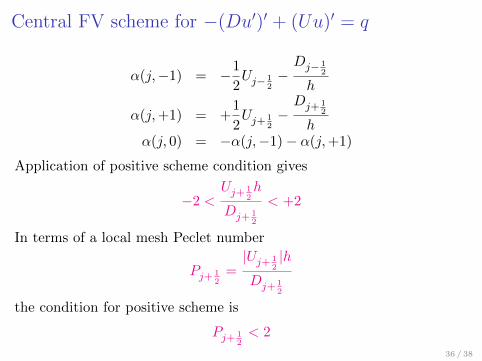
Central FV scheme for −(Du′)′ + (Uu)′ = q
α(j,−1) = −1
2Uj− 1
2−Dj− 1
2
h
α(j,+1) = +1
2Uj+ 1
2−Dj+ 1
2
hα(j, 0) = −α(j,−1)− α(j,+1)
Application of positive scheme condition gives
−2 <Uj+ 1
2h
Dj+ 12
< +2
In terms of a local mesh Peclet number
Pj+ 12
=|Uj+ 1
2|h
Dj+ 12
the condition for positive scheme is
Pj+ 12< 2
36 / 38
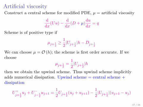
Artificial viscosityConstruct a central scheme for modified PDE, µ = artificial viscosity
d
dx(Uu)− d
dx(D + µ)
du
dx= q
Scheme is of positive type if
µj+ 12≥ 1
2|Uj+ 1
2|h−Dj+ 1
2
We can choose µ = O (h); the scheme is first order accurate. If wechoose
µj+ 12
=1
2|Uj+ 1
2|h
then we obtain the upwind scheme. Thus upwind scheme implicitlyadds numerical dissipation. Upwind scheme = central scheme +dissipation
U+j+ 1
2
uj + U−j− 1
2
uj+1 =1
2Uj+ 1
2(uj + uj+1)− 1
2|Uj+ 1
2|(uj+1 − uj)
37 / 38
Hybrid scheme
For convective flux F = Uu, use blending of upwind and centralscheme; switch locally based on local mesh Peclet number
F cj+ 1
2
=1
2Uj+ 1
2(uj + uj+1), F u
j+ 12
= U+j+ 1
2
uj + U−j− 1
2
uj+1
Switching function
s(P ) =
0, P < 2
1, P ≥ 2
Hybrid scheme
Fj+ 12
= s(Pj+ 12)F u
j+ 12
+ [1− s(Pj+ 12)]F c
j+ 12
Preferable to use a smooth switching function. Hybrid schemesintroduced by Spalding (1972) and Patankar (1980).
38 / 38


![A boundary value problem for conjugate conductivity equations · The GASPT theory has been investigated by many authors, among whom Weinstein [28{31], Vekua [27], Gilbert [12{15],](https://static.fdocument.org/doc/165x107/5f5a2f39930dab2c133bad38/a-boundary-value-problem-for-conjugate-conductivity-equations-the-gaspt-theory-has.jpg)