Numerical Solution of Partial Differential...
40
Numerical Solution of Partial Differential Equations Praveen. C [email protected] Tata Institute of Fundamental Research Center for Applicable Mathematics Bangalore 560065 http://math.tifrbng.res.in 31 January 2009 Praveen. C (TIFR-CAM) Numerical PDE Jan 31, 2009 1 / 40
Transcript of Numerical Solution of Partial Differential...
Numerical Solution of Partial Differential Equations
Praveen. [email protected]
Tata Institute of Fundamental ResearchCenter for Applicable Mathematics
Bangalore 560065http://math.tifrbng.res.in
31 January 2009
Praveen. C (TIFR-CAM) Numerical PDE Jan 31, 2009 1 / 40
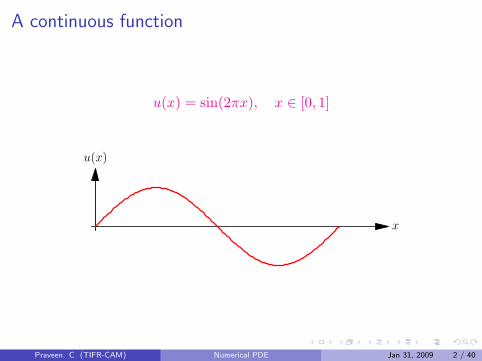
A continuous function
u(x) = sin(2πx), x ∈ [0, 1]
x
u(x)
Praveen. C (TIFR-CAM) Numerical PDE Jan 31, 2009 2 / 40
Space of continuous functions
• C([0, 1]) = Space of continuous functions
• C([0, 1]) has infinitely many elements in it=⇒ We say it is infinite dimensional
• Example:u(x) = sin(2πx) is an element of C([0, 1])
• A computer has finite memory=⇒ It cannot represent infinite dimensional objects
Hence we need to approximate an infinite dimensional object using a finitedimensional space
Praveen. C (TIFR-CAM) Numerical PDE Jan 31, 2009 3 / 40
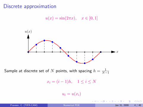
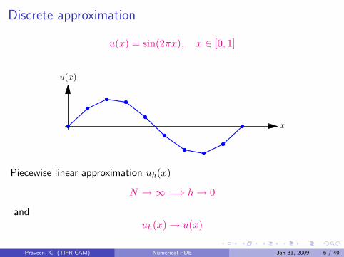
Discrete approximation
u(x) = sin(2πx), x ∈ [0, 1]
x
u(x)
Sample at discrete set of N points, with spacing h = 1N−1
xi = (i− 1)h, 1 ≤ i ≤ N
ui = u(xi)
Praveen. C (TIFR-CAM) Numerical PDE Jan 31, 2009 4 / 40
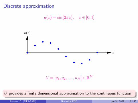
Discrete approximation
u(x) = sin(2πx), x ∈ [0, 1]
x
u(x)
U = [u1, u2, . . . , uN ] ∈ RN
U provides a finite dimensional approximation to the continuous function
Praveen. C (TIFR-CAM) Numerical PDE Jan 31, 2009 5 / 40
Discrete approximation
u(x) = sin(2πx), x ∈ [0, 1]
x
u(x)
Piecewise linear approximation uh(x)
N →∞ =⇒ h→ 0
anduh(x)→ u(x)
Praveen. C (TIFR-CAM) Numerical PDE Jan 31, 2009 6 / 40
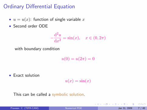
Ordinary Differential Equation
• u = u(x): function of single variable x
• Second order ODE
−d2u
dx2= sin(x), x ∈ (0, 2π)
with boundary condition
u(0) = u(2π) = 0
• Exact solutionu(x) = sin(x)
This can be called a symbolic solution.
Praveen. C (TIFR-CAM) Numerical PDE Jan 31, 2009 7 / 40
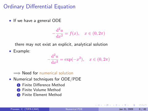
Ordinary Differential Equation
• If we have a general ODE
−d2u
dx2= f(x), x ∈ (0, 2π)
there may not exist an explicit, analytical solution
• Example:
−d2u
dx2= exp(−x2), x ∈ (0, 2π)
=⇒ Need for numerical solution
• Numerical techniques for ODE/PDE
1 Finite Difference Method2 Finite Volume Method3 Finite Element Method
Praveen. C (TIFR-CAM) Numerical PDE Jan 31, 2009 8 / 40
Finite Difference Method• Consider a general ODE
−d2u
dx2= f(x), x ∈ (a, b)
with boundary conditions
u(a) = ua, u(b) = ub
• Instead of finding a function that solves the ODE, find a discreteapproximation to the solution
• Divide computational domain (a, b) into N + 1 intervals each of size
h =b− aN + 1
• Computational grid
xi = ih, 0 ≤ i ≤ N + 1
Praveen. C (TIFR-CAM) Numerical PDE Jan 31, 2009 9 / 40
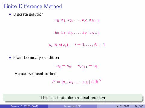
Finite Difference Method
• Discrete solutionx0, x1, x2, . . . , xN , xN+1
u0, u1, u2, . . . , uN , uN+1
ui ≈ u(xi), i = 0, . . . , N + 1
• From boundary condition
u0 = ua, uN+1 = ub
Hence, we need to find
U = [u1, u2, . . . , uN ] ∈ RN
This is a finite dimensional problem
Praveen. C (TIFR-CAM) Numerical PDE Jan 31, 2009 10 / 40
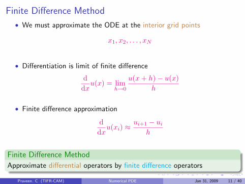
Finite Difference Method
• We must approximate the ODE at the interior grid points
x1, x2, . . . , xN
• Differentiation is limit of finite difference
ddxu(x) = lim
h→0
u(x+ h)− u(x)h
• Finite difference approximation
ddxu(xi) ≈
ui+1 − ui
h
Finite Difference Method
Approximate differential operators by finite difference operators
Praveen. C (TIFR-CAM) Numerical PDE Jan 31, 2009 11 / 40
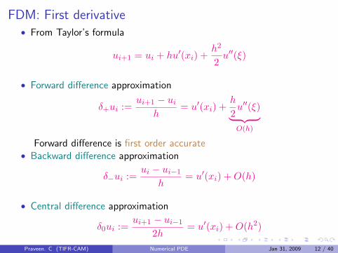
FDM: First derivative• From Taylor’s formula
ui+1 = ui + hu′(xi) +h2
2u′′(ξ)
• Forward difference approximation
δ+ui :=ui+1 − ui
h= u′(xi) +
h
2u′′(ξ)︸ ︷︷ ︸O(h)
Forward difference is first order accurate• Backward difference approximation
δ−ui :=ui − ui−1
h= u′(xi) +O(h)
• Central difference approximation
δ0ui :=ui+1 − ui−1
2h= u′(xi) +O(h2)
Praveen. C (TIFR-CAM) Numerical PDE Jan 31, 2009 12 / 40
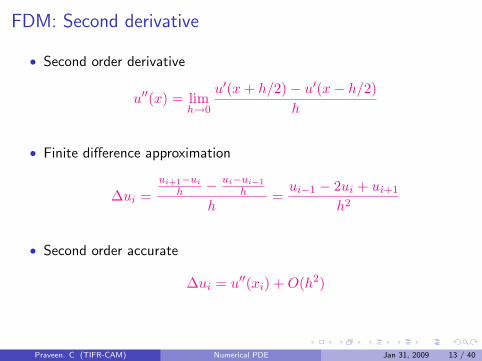
FDM: Second derivative
• Second order derivative
u′′(x) = limh→0
u′(x+ h/2)− u′(x− h/2)h
• Finite difference approximation
∆ui =ui+1−ui
h − ui−ui−1
h
h=ui−1 − 2ui + ui+1
h2
• Second order accurate
∆ui = u′′(xi) +O(h2)
Praveen. C (TIFR-CAM) Numerical PDE Jan 31, 2009 13 / 40
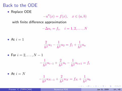
Back to the ODE• Replace ODE
−u′′(x) = f(x), x ∈ (a, b)
with finite difference approximation
−∆ui = fi, i = 1, 2, . . . , N
• At i = 12h2u1 −
1h2u2 = f1 +
1h2ua
• For i = 2, . . . , N − 1
− 1h2ui−1 +
2h2ui −
1h2ui+1 = fi
• At i = N
− 1h2uN−1 +
2h2uN = fN +
1h2ub
Praveen. C (TIFR-CAM) Numerical PDE Jan 31, 2009 14 / 40
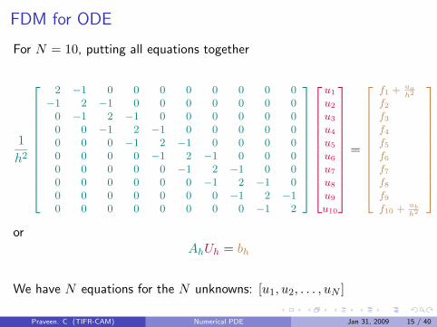
FDM for ODE
For N = 10, putting all equations together
1h2
2 −1 0 0 0 0 0 0 0 0−1 2 −1 0 0 0 0 0 0 0
0 −1 2 −1 0 0 0 0 0 00 0 −1 2 −1 0 0 0 0 00 0 0 −1 2 −1 0 0 0 00 0 0 0 −1 2 −1 0 0 00 0 0 0 0 −1 2 −1 0 00 0 0 0 0 0 −1 2 −1 00 0 0 0 0 0 0 −1 2 −10 0 0 0 0 0 0 0 −1 2
u1
u2
u3
u4
u5
u6
u7
u8
u9
u10
=
f1 + uah2
f2
f3
f4
f5
f6
f7
f8
f9
f10 + ubh2
or
AhUh = bh
We have N equations for the N unknowns: [u1, u2, . . . , uN ]
Praveen. C (TIFR-CAM) Numerical PDE Jan 31, 2009 15 / 40
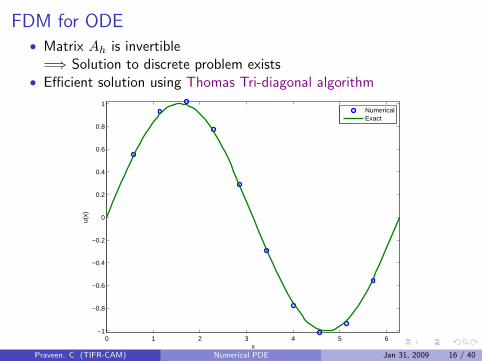
FDM for ODE• Matrix Ah is invertible
=⇒ Solution to discrete problem exists• Efficient solution using Thomas Tri-diagonal algorithm
0 1 2 3 4 5 6−1
−0.8
−0.6
−0.4
−0.2
0
0.2
0.4
0.6
0.8
1
x
u(x)
NumericalExact
Praveen. C (TIFR-CAM) Numerical PDE Jan 31, 2009 16 / 40
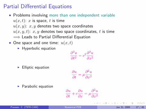
Partial Differential Equations
• Problems involving more than one independent variableu(x, t): x is space, t is timeu(x, y): x, y denotes two space coordinatesu(x, y, t): x, y denotes two space coordinates, t is time=⇒ Leads to Partial Differential Equation
• One space and one time: u(x, t)I Hyperbolic equation
∂2u
∂t2= c2
∂2u
∂x2
I Elliptic equation∂u
∂t= µ
∂2u
∂x2
I Parabolic equation∂u
∂t+ c
∂u
∂x= µ
∂2u
∂x2
Praveen. C (TIFR-CAM) Numerical PDE Jan 31, 2009 17 / 40
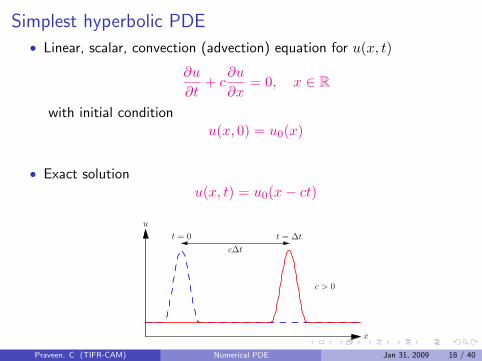
Simplest hyperbolic PDE
• Linear, scalar, convection (advection) equation for u(x, t)
∂u
∂t+ c
∂u
∂x= 0, x ∈ R
with initial conditionu(x, 0) = u0(x)
• Exact solutionu(x, t) = u0(x− ct)
x
u
t = 0 t = ∆t
c∆t
c > 0
Praveen. C (TIFR-CAM) Numerical PDE Jan 31, 2009 18 / 40
Hyperbolic PDE
Wave
A phenomenon in which some recognizable feature propagates with arecognizable speed
Hyperbolic PDE
A PDE which has wave-like solutions
• Waves propagate in specific directions:
• Linear, convection equation
I c > 0 =⇒ wave moves to the rightI c < 0 =⇒ wave moves to the leftI c is the speed at which waves propagateI Finite speed of propagationI Preserves shape of initial condition
Praveen. C (TIFR-CAM) Numerical PDE Jan 31, 2009 19 / 40

Hyperbolic PDE• Scalar, convection equation(
∂
∂t+ c
∂
∂x
)u = 0
contains one wave• Second order wave equation
∂2u
∂t2= c2
∂2u
∂x2
I can be factored (∂
∂t+ c
∂
∂x
)(∂
∂t− c ∂
∂x
)u = 0
I contains two waves, with speed +c and −cI In fact, general solution is
u(x, t) = f(x− ct) + g(x+ ct)
Praveen. C (TIFR-CAM) Numerical PDE Jan 31, 2009 20 / 40
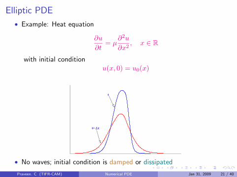
Elliptic PDE
• Example: Heat equation
∂u
∂t= µ
∂2u
∂x2, x ∈ R
with initial conditionu(x, 0) = u0(x)
∆ tt+
t
• No waves; initial condition is damped or dissipated
Praveen. C (TIFR-CAM) Numerical PDE Jan 31, 2009 21 / 40
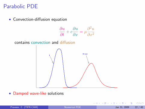
Parabolic PDE
• Convection-diffusion equation
∂u
∂t+ c
∂u
∂x= µ
∂2u
∂x2
contains convection and diffusion
∆ tt+t
• Damped wave-like solutions
Praveen. C (TIFR-CAM) Numerical PDE Jan 31, 2009 22 / 40
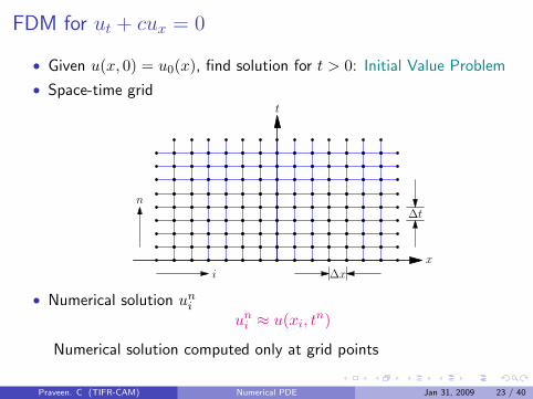
FDM for ut + cux = 0
• Given u(x, 0) = u0(x), find solution for t > 0: Initial Value Problem
• Space-time grid
x
t
i
n
∆x
∆t
• Numerical solution uni
uni ≈ u(xi, t
n)
Numerical solution computed only at grid points
Praveen. C (TIFR-CAM) Numerical PDE Jan 31, 2009 23 / 40
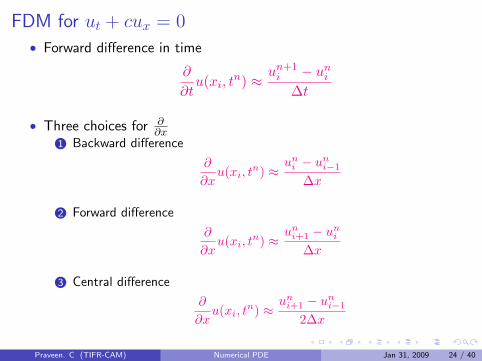
FDM for ut + cux = 0
• Forward difference in time
∂
∂tu(xi, t
n) ≈un+1
i − uni
∆t
• Three choices for ∂∂x
1 Backward difference
∂
∂xu(xi, t
n) ≈un
i − uni−1
∆x
2 Forward difference
∂
∂xu(xi, t
n) ≈un
i+1 − uni
∆x
3 Central difference
∂
∂xu(xi, t
n) ≈un
i+1 − uni−1
2∆x
Praveen. C (TIFR-CAM) Numerical PDE Jan 31, 2009 24 / 40
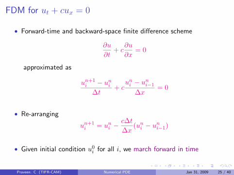
FDM for ut + cux = 0
• Forward-time and backward-space finite difference scheme
∂u
∂t+ c
∂u
∂x= 0
approximated as
un+1i − un
i
∆t+ c
uni − un
i−1
∆x= 0
• Re-arranging
un+1i = un
i −c∆t∆x
(uni − un
i−1)
• Given initial condition u0i for all i, we march forward in time
Praveen. C (TIFR-CAM) Numerical PDE Jan 31, 2009 25 / 40
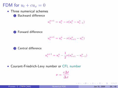
FDM for ut + cux = 0• Three numerical schemes
1 Backward difference
un+1i = un
i − ν(uni − un
i−1)
2 Forward difference
un+1i = un
i − ν(uni+1 − un
i )
3 Central difference
un+1i = un
i −12ν(un
i+1 − uni−1)
• Courant-Friedrich-Levy number or CFL number
ν =c∆t∆x
Praveen. C (TIFR-CAM) Numerical PDE Jan 31, 2009 26 / 40
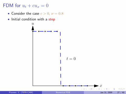
FDM for ut + cux = 0
• Consider the case c > 0, ν = 0.8• Initial condition with a step
x
u
t = 0
Praveen. C (TIFR-CAM) Numerical PDE Jan 31, 2009 27 / 40
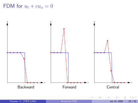
FDM for ut + cux = 0
x
u
x
u
x
u
Backward Forward Central
Praveen. C (TIFR-CAM) Numerical PDE Jan 31, 2009 28 / 40
FDM for ut + cux = 0
• For stable schemes: ‖un‖ remains bounded
• For unstable schemes: ‖un‖ → ∞ as n→∞• For c > 0
Backward =⇒ stableForward =⇒ unstableCentral =⇒ unstable
• For c < 0Backward =⇒ unstableForward =⇒ stableCentral =⇒ unstable
Hyperbolic problems
Finite difference scheme must be chosen based on the sign/direction ofwaves present in the problem
Praveen. C (TIFR-CAM) Numerical PDE Jan 31, 2009 29 / 40
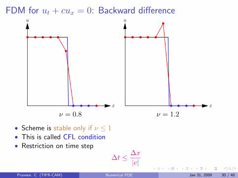
FDM for ut + cux = 0: Backward difference
x
u
x
u
ν = 0.8 ν = 1.2
• Scheme is stable only if ν ≤ 1• This is called CFL condition• Restriction on time step
∆t ≤ ∆x|c|
Praveen. C (TIFR-CAM) Numerical PDE Jan 31, 2009 30 / 40
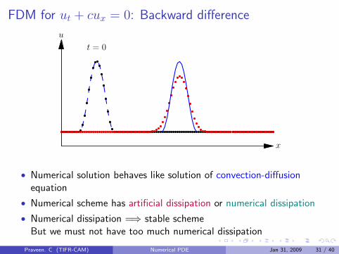
FDM for ut + cux = 0: Backward difference
x
u
t = 0
• Numerical solution behaves like solution of convection-diffusionequation
• Numerical scheme has artificial dissipation or numerical dissipation
• Numerical dissipation =⇒ stable schemeBut we must not have too much numerical dissipation
Praveen. C (TIFR-CAM) Numerical PDE Jan 31, 2009 31 / 40
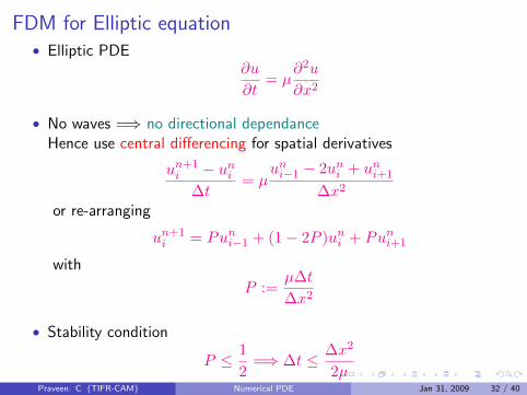
FDM for Elliptic equation• Elliptic PDE
∂u
∂t= µ
∂2u
∂x2
• No waves =⇒ no directional dependanceHence use central differencing for spatial derivatives
un+1i − un
i
∆t= µ
uni−1 − 2un
i + uni+1
∆x2
or re-arranging
un+1i = Pun
i−1 + (1− 2P )uni + Pun
i+1
with
P :=µ∆t∆x2
• Stability condition
P ≤ 12
=⇒ ∆t ≤ ∆x2
2µPraveen. C (TIFR-CAM) Numerical PDE Jan 31, 2009 32 / 40
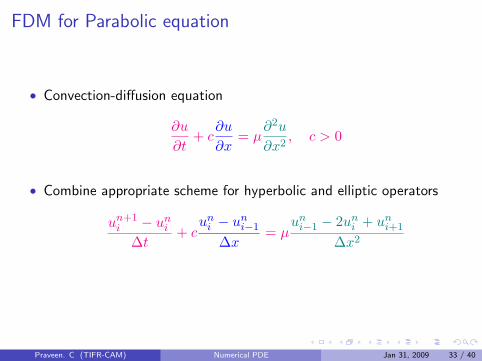
FDM for Parabolic equation
• Convection-diffusion equation
∂u
∂t+ c
∂u
∂x= µ
∂2u
∂x2, c > 0
• Combine appropriate scheme for hyperbolic and elliptic operators
un+1i − un
i
∆t+ c
uni − un
i−1
∆x= µ
uni−1 − 2un
i + uni+1
∆x2
Praveen. C (TIFR-CAM) Numerical PDE Jan 31, 2009 33 / 40
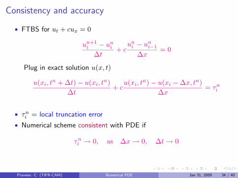
Consistency and accuracy
• FTBS for ut + cux = 0
un+1i − un
i
∆t+ c
uni − un
i−1
∆x= 0
Plug in exact solution u(x, t)
u(xi, tn + ∆t)− u(xi, t
n)∆t
+ cu(xi, t
n)− u(xi −∆x, tn)∆x
= τni
• τni = local truncation error
• Numerical scheme consistent with PDE if
τni → 0, as ∆x→ 0, ∆t→ 0
Praveen. C (TIFR-CAM) Numerical PDE Jan 31, 2009 34 / 40
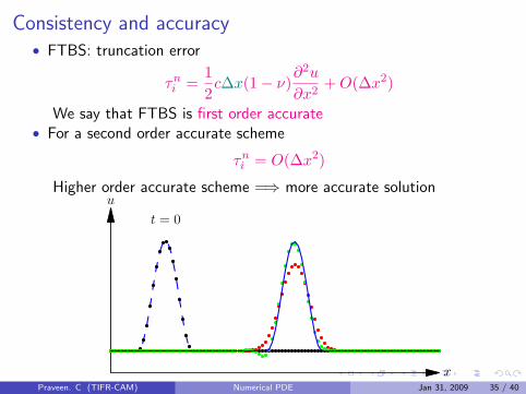
Consistency and accuracy• FTBS: truncation error
τni =
12c∆x(1− ν)
∂2u
∂x2+O(∆x2)
We say that FTBS is first order accurate• For a second order accurate scheme
τni = O(∆x2)
Higher order accurate scheme =⇒ more accurate solution
x
u
t = 0
Praveen. C (TIFR-CAM) Numerical PDE Jan 31, 2009 35 / 40
Convergence
Does the numerical solution converge to the exact solution as the grid isrefined ?
∆x→ 0, ∆t→ 0 =⇒ uni → u(xi, t
n)
Lax-Richtmyer Equivalence theorem
A consistent finite difference scheme for a PDE for which the initial valueproblem is well-posed is convergent if and only if it is stable
Praveen. C (TIFR-CAM) Numerical PDE Jan 31, 2009 36 / 40
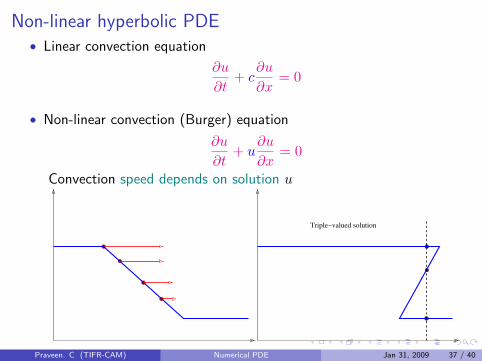
Non-linear hyperbolic PDE• Linear convection equation
∂u
∂t+ c
∂u
∂x= 0
• Non-linear convection (Burger) equation
∂u
∂t+ u
∂u
∂x= 0
Convection speed depends on solution u
Triple−valued solution
Praveen. C (TIFR-CAM) Numerical PDE Jan 31, 2009 37 / 40
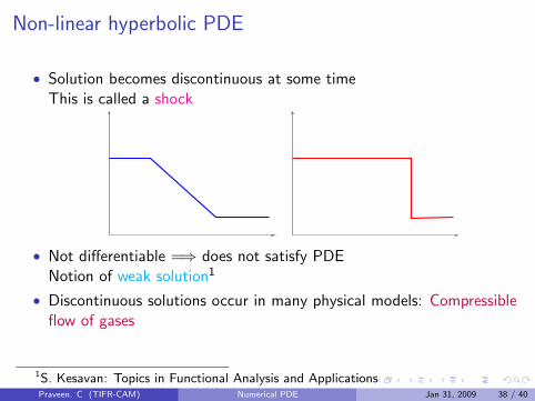
Non-linear hyperbolic PDE
• Solution becomes discontinuous at some timeThis is called a shock
• Not differentiable =⇒ does not satisfy PDENotion of weak solution1
• Discontinuous solutions occur in many physical models: Compressibleflow of gases
1S. Kesavan: Topics in Functional Analysis and ApplicationsPraveen. C (TIFR-CAM) Numerical PDE Jan 31, 2009 38 / 40
Summary of numerical method
Choice of numerical scheme based on physics in the problem:convection and/or diffusion
• Discretize PDE using finite differences
• Check consistency of numerical scheme
• Check stability of numerical scheme
• Check convergence of numerical solution to exact solution
• Validate numerical scheme against available exact solutions
Praveen. C (TIFR-CAM) Numerical PDE Jan 31, 2009 39 / 40
References
• F. StrikwerdaFinite difference schemes and partial differential equations
• A. IserlesA first course in the numerical analysis of differential equations
Praveen. C (TIFR-CAM) Numerical PDE Jan 31, 2009 40 / 40
![Dynamical Models of Dark Energy - WordPress.com · Universe is accelerating [1, 2]. The name given to this phenomenon does much to convey the mystery which still surrounds it; we](https://static.fdocument.org/doc/165x107/5f0634417e708231d416d152/dynamical-models-of-dark-energy-universe-is-accelerating-1-2-the-name-given.jpg)

![HIGH FREQUENCY OSCILLATIONS OF FIRST EIGENMODES IN ...Encyclopedia of Vibration: [We observe] a phenomenon which is particular to many deep shells, namely that the lowest natural frequency](https://static.fdocument.org/doc/165x107/5e842943dcac337abb39c6f3/high-frequency-oscillations-of-first-eigenmodes-in-encyclopedia-of-vibration.jpg)