Boundary element modelling to solve the Grad … · Boundary element modelling to solve the...

Instructions for use

Title Boundary element modelling to solve the Grad‒Shafranov equation as an axisymmetric problem

Author(s) Itagaki, Masafumi; Fukunaga, Takaaki

Citation Engineering Analysis with Boundary Elements, 30(9): 746-757

Issue Date 2006-09

Doc URL http://hdl.handle.net/2115/14922

Type article (author version)

File Information EABE30-9.pdf

Hokkaido University Collection of Scholarly and Academic Papers : HUSCAP

https://eprints.lib.hokudai.ac.jp/dspace/about.en.jsp

1

Boundary element modelling to solve

the Grad-Shafranov equation as an axisymmetric problem

Masafumi ITAGAKI, Takaaki FUKUNAGA

Graduate School of Engineering, Hokkaido University,

Kita 13, Nishi 8, Kita-ku, Sapporo 060-8628, JAPAN

Tel. +81-11-706-6659, Fax. +81-11-747-9366

E-mail: [email protected]

This paper contains

24 pages of text

and 9 figures.

2

Abstract

The Grad-Shafranov equation describes the magnetic flux distribution of plasma in an axisymmetric

system like a tokamak-type nuclear fusion device. The equation is transformed into an equivalent

boundary integral equation by expanding the inhomogeneous term related to the plasma current into

a polynomial. In the present research, the singularity of the fundamental solution, which consists of

two elliptic integrals, and the properties of singular integrals have been minutely investigated. The

discontinuous quadratic boundary elements have been introduced to give an accurate solution with a

small number of boundary elements. Ampere’s circuital law has been applied to estimate the total

plasma current from the boundary integral of the poloidal field, and based on this idea, a new

scheme to calculate the eigenvalue has also been proposed.

3

1. Introduction

In a tokamak-type nuclear fusion device, the plasma particles are confined in a torus vacuum

vessel by a magnetic field. The confinement performance of plasma depends on the magnetic field

configuration in the vessel. The torus plasma in a 3-dimensional (3-D) space can be regarded as

axisymmetric in the toroidal direction, so that the magnetic field configuration is often analyzed

using the Grad-Shafranov equation for a 2-D, r-z system. This equation describes the

magnetohydrodynamic (MHD) equilibrium of plasma in terms of the poloidal magnetic flux ψ [1]．

The boundary element method (BEM) [2] is well suited for solving the Grad-Shadranov equation,

since an online analysis requires frequent preparation and modification of geometric data following

the change in plasma shape during the operation of an actual fusion device. The inhomogeneous

term related to the plasma current in the equation hampers the transformation of the equation into the

boundary integral one. Itagaki et al. [3] successfully transformed the domain integral caused by the

inhomogeneous term into an equivalent boundary integral, by expanding the inhomogeneous term

into a 2-D polynomial, using a particular solution corresponding to the polynomial, and applying

Green’s second identity. Further, Itagaki et al. [4] applied the above boundary element formulation to

an inverse analysis where the plasma current density profile was reconstructed from signals of

magnetic sensors located outside the plasma. However, only the constant boundary element

approximation, as the simplest discretization model, was used in the above two papers.

As the Grad-Shafranov equation deals with the axisymmetric problem, the fundamental solution

has a somewhat complicated mathematical form that includes elliptic integrals. Accordingly, one

needs to investigate carefully the singularity of this fundamental solution and also the properties of

singular integrals. Unfortunately these aspects were not discussed in the above two papers; they have

not yet been reported.

In the present paper, the authors clarify the characteristics of the fundamental solution and its

4

boundary integrals, which are peculiar to the Grad-Shafranov equation. Some points to note when

performing numerical integrations are also given. The discontinuous (non-conforming) quadratic

boundary elements [5] have been introduced to realize accurate solutions with a small number of

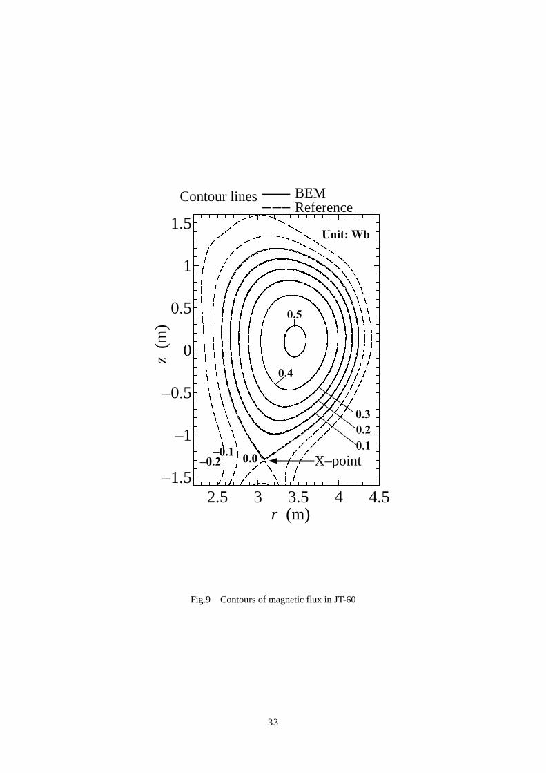
boundary elements. Here, the reason why the authors concern themselves with the discontinuous

elements is that one needs to deal with the so-called “X-point”, a type of corner point having two

normal derivatives of magnetic flux (not differentiable), which will be later found in Fig.9.

Itagaki et al. [3,4] evaluated the total plasma current by directly integrating the

polynomial-expanded inhomogeneous term. In the present work the authors propose an alternative

technique based on Ampere’s circuital law, i.e., a boundary integral of the poloidal field. Utilizing

this new technique, a smart method of eigenvalue computation is also proposed. Numerical

examples are given in Section 6.

2. Boundary integral equation for the Grad-Shafranov equation

For an axisymmetric (r,z) system, the differential form of Ampere’s law 0µ = ∇ ×j B can be

reduced to a partial differential equation

2*

02

1r rjr r r z ϕψ ψ µ

∂ ∂ ∂ −∆ ≡ − + = ∂ ∂ ∂ (1)

in terms of magnetic flux ψ [1]．Here, jϕ denotes the toroidal component of of the plasma

current, and 0µ is the permeability of a vacuum. Applying also the equilibrium condition that the

plasma pressure is balanced by the magnetic forces, p× = ∇j B , Eq.(1) is rewritten in the form [1]

2* 2

0 0 ,2

dp d Fr rjd d ϕψ µ µψ ψ

−∆ = + ≡

(2)

where p is the plasma pressure and F is the poloidal current function. Equation (2) is called the

Grad-Shafranov equation, however, the authors call both Eqs.(1) and (2) the Grad- Shafranov

equation in the present paper for convenience.

5

One here introduces the fundamental solution *ψ that satisfies a subsidiary equation

* * ,irψ δ−∆ = (3)

where Dirac’s delta function iδ means ( ) ( )r a z bδ δ− − with the spike at the point i having the

coordinates ( , )a b . Physically, Eq.(3) describes the magnetic flux for an arbitrary field point ( , )r z

caused by a unit toroidal current located at the point ( , )a b . The detailed form of the fundamental

solution is given by

( ) ( )2

* 12

ar k K k E kk

ψπ

= − −

(4)

with

( ) ( )

22 2

4arkr a z b

=+ + −

, (5)

where ( )K k and ( )E k are the complete elliptic integrals of the first and second kinds,

respectively.

Itagaki et al [3] showed that the above Grad-Shafranov equation can be transformed into an

equivalent boundary-only integral equation in terms of the plasma boundary Γ ,

* * * ( , ) ( , ) *( , )

,,

l m l ml m

i i l m i il m

c d c dr n r n r n r n

ψ ψ ψ ψ ψ ϕ ϕ ψψ α ϕΓ Γ

∂ ∂ ∂ ∂ − − Γ = − − Γ ∂ ∂ ∂ ∂ ∑∫ ∫

, (6)

by assuming a polynomial expansion of the RHS of Eq.(1):

0 ,,

. ( 0, 0)l ml m

l mr j l mϕµ α ξ η≈ ≥ ≥∑ . (7)

Here, ξ and η are dimensionless coordinates / rr Lξ = and 0( ) / zz z Lη = − , respectively

with appropriate constants rL , zL and 0z . Note here that Eq.(7) itself does not include any

information related to the equilibrium condition, × p= ∇J B , explicitly. In an actual analysis, one

needs to add a restriction to consider this equilibrium condition, as will be shown later in Eq.(56).

The constant ic in Eq.(6) depends on the local boundary geometry under consideration:

1.0ic = for an internal point, while 1/ 2ic = on a smooth boundary (see also section 4.3). The

6

quantity ( , )l mϕ means a particular solution that satisfies the Grad-Shafranov equation with a

monomial source:

* ( , ) 0 . ( 0, 0)l m

l m l m

r z

z zr l mL L

ϕ ξ η −−∆ = = ≥ ≥

(8)

The detailed form of ( , )l mϕ is written as an infinite series [3]:

22 2

( , )

1 1

( 2 2)( 2 )1( 1)( 2) ( 2 1)( 2 2)

l m kl m z z

k s r

L Ll s l sm m m s m s L

ξ η ηϕξ

+ ∞

= =

− + − = − + − + + + + + + ∑∏ . (9)

3. Discretization

3.1 Constant boundary elements

The constant boundary element can be regarded as the simplest ‘discontinuous’ element, which is

convenient to model the plasma boundary including the X-point, since the value of a physical

quantity is assumed to be constant on each element and equal to the value at the mid-node of the

element. In this case Eq.(6) for a given ‘ i ’ point becomes in a discretized form

* *

1 1

* ( , ) ( , ) *( , )

,, 1

1

j j

j

N N

i i jj jj

l m l mNl m

l m i il m j

c d dn r r n

c dr n r n

ψ ψ ψψ ψ

ψ ϕ ϕ ψα ϕ

= =Γ Γ

= Γ

∂ ∂ − Γ + Γ ∂ ∂

∂ ∂ = − − Γ ∂ ∂

∑ ∑∫ ∫

∑ ∑ ∫ , (10)

where N denotes the total number of boundary elements. Equation (10) can be rewritten as

1 1

ˆ ( 1,2, , )N N

i i ij ij j ij jj

c G H Q i Nnψψ ψ

= =

∂ − + = = ∂ ∑ ∑ ! , (11)

when one defines the quantities

* *1ˆ, ,j j

ij ijG d H dr r n

ψ ψΓ Γ

∂= Γ = Γ∂∫ ∫ (12)

and

7

* ( , ) ( , ) *( , )

,, 1 j

l m l mNl m

i l m i il m j

Q c dr n r n

ψ ϕ ϕ ψα ϕ= Γ

∂ ∂ = − − Γ ∂ ∂ ∑ ∑ ∫ . (13)

Now one also defines ijH as

ˆ ( )ˆ ( ).

ijij

i ii

H i jH

c H i j

≠= + =

(14)

It is known that, when the Laplace equation is solved using straight line elements such as constant or

linear boundary elements, ˆiiH is zero due to the orthogonality of the integral path and the normal

direction [2]. This is not true when solving the Grad-Shafranov equation for the reason described

later in Section 4.2.

Using the above notation, Eq.(11) is further rewritten as

1 1

N N

ij j ij ij j j

H G Qnψψ

= =

∂ − = ∂ ∑ ∑ , (15)

and the whole set in matrix form becomes

− =Hψ Gq Q . (16)

3.2 Discontinuous quadratic elements

The geometrical shape of a quadratic element is expressed as

1 1 2 2 3 3( ) ( ) ( ) ( )f f fζ ζ ζ ζ= + +x x x x (17)

in terms of three shape functions

1 2 31 1( ) ( 1), ( ) (1 )(1 ), ( ) ( 1) ( 1 1)2 2

f f fζ ζ ζ ζ ζ ζ ζ ζ ζ ζ= − = − + = + − ≤ ≤ (18)

with the coordinates at three mesh points, 1 2 3, ,x x x , on the element. The quantities ψ and

/ nψ∂ ∂ are also interpolated as

1 1 2 2 3 3( ) ( ) ( ) ( )ψ ζ ζ ψ ζ ψ ζ ψ= Φ + Φ + Φ (19a)

and

8

1 2 31 2 3

( ) ( ) ( ) ( )n n n n

ψ ζ ψ ψ ψζ ζ ζ∂ ∂ ∂ ∂ = Φ + Φ + Φ ∂ ∂ ∂ ∂ . (19b)

The interpolation functions for the discontinuous quadratic elements, however, are different from the

shape functions of Eq.(18), since the node points at both ends are shifted inwards. The interpolation

functions adopted here have the forms

1 2 33 3 3 3 3 3( ) 1 , ( ) 1 1 , ( ) 14 2 2 2 4 2

ζ ζ ζ ζ ζ ζ ζ ζ ζ Φ = − Φ = − + Φ = +

. (20)

The boundary integrals on jΓ can then be discretized as

* *

1 1 2 2 3 3

1 , 1 2 , 2 3 , 3

1( ) ( ) ( )

,j j

jj j j

j i j j i j j i j

d dr n r n

h h h

ψ ψ ψζ ψ ζ ψ ζ ψ

ψ ψ ψΓ Γ

∂ ∂Γ = Φ + Φ + Φ Γ∂ ∂

= + +

∫ ∫ (21a)

and

* *

1 2 31 2 3

, 1 , 2 , 31 2 3

( ) ( ) ( )

,

j jj j j j

i j i j i jj j j

d dr n n n n r

g g gn n n

ψ ψ ψ ψ ψ ψζ ζ ζ

ψ ψ ψΓ Γ

∂ ∂ ∂ ∂ Γ = Φ + Φ + Φ Γ ∂ ∂ ∂ ∂ ∂ ∂ ∂ = + + ∂ ∂ ∂

∫ ∫

(21b)

where

* * *

, 1 1 , 2 2 , 3 31 1 1( ) , ( ) , ( )

j j j

i j i j i jh d h d h dr n r n r n

ψ ψ ψζ ζ ζΓ Γ Γ

∂ ∂ ∂= Φ Γ = Φ Γ = Φ Γ∂ ∂ ∂∫ ∫ ∫ (22a)

and

* * *

, 1 1 , 2 2 , 3 3( ) , ( ) , ( )j j j

i j i j i jg d g d g dr r r

ψ ψ ψζ ζ ζΓ Γ Γ

= Φ Γ = Φ Γ = Φ Γ∫ ∫ ∫ . (22b)

The total number of node points is 3N corresponding to a total of N boundary elements. Now

one defines the quantities

, 1 , 1

, 2 , 2

, 3 , 3

( 1 1,4,7, ,3 2) ( 1 1,4,7, ,3 2)ˆ ( 2 2,5,8, ,3 1), ( 2 2,5,8, ,3 1)

( 3 3,6,9, ,3 ) ( 3 3,6,9, ,3 ) ,

i j i j

ij i j ij i j

i j i j

h j N g j NH h j N G g j N

h j N g j N

= − = − = = − = = − = =

! !! !! !

(23)

* ( , ) ( , ) *( , )

,, 1 j

l m l mNl m

i l m i il m j

Q c dr n r n

ψ ϕ ϕ ψα ϕ= Γ

∂ ∂ = − − Γ ∂ ∂ ∑ ∑ ∫ , (24)

and

9

ˆ ( )ˆ ( )

ijij

i ii

H i jH

c H i j

≠= + =

. (25)

It should be noted here again that ˆ 0iiH ≠ even if the shape of a boundary element is a straight line.

The original boundary integral equation is now reduced to the discretized form

3 3

1 1

( 1, 2, ,3 ).N N

ij j ij ij j j

H G Q i Nnψψ

= =

∂ − = = ∂ ∑ ∑ ! (26)

4. Remarks on the singular integrals

When the source point ( , )a b and the field point ( , )r z are located far from each other, the

ordinary Gaussian quadrature gives an acceptable accuracy for each boundary integral in Eq.(6).

However, if the points are close to each other, especially when the source point is located within the

boundary element under consideration, special care must be taken concerning singular integrals. The

fundamental solution given by Eq.(4) contains the two elliptic integrals. When the field point

approaches the source point, these elliptic integrals can be approximated as [6]

22

1 16 1( ) log log log(4 4 )2 1

K k ark

εε

≈ = + + − (27a)

and

( ) 1E k ≈ , (27b)

where 2 2( ) ( )r a z bε = − + − is the distance between the source point and the field point. In this

section, starting with Eqs.(27a) and (27b), one investigates the singularity of the fundamental

solution, the properties of singular integrals, and a technique to eliminate the singularity.

4.1 Integrals in terms of * / rψ

Substituting Eqs.(27a) and (27b) into Eq.(4), the fundamental solution becomes approximated as

10

2 2* 2

2

4 2 1 1log log(4 4 ) 1 log log82 4 2 2

ar ar a a aar aar

ε εψ επ ε ε π ε π π

+ + ≈ + + − → + − + (28)

when , 0r a ε→ → . That is, this fundamental solution represents only a ‘weak’ singularity.

Consequently, the boundary integrals in terms of * / rψ can be performed as

* * 1 1 1 1log log2 2

d d dr r

ψ ψπ ε π εΓ Γ Γ

Γ = − Γ + Γ

∫ ∫ ∫ (29a)

and

* * 1 1 1 1log log2 2

i id d dr n r n n n

ϕ ϕψ ϕ ψ ϕπ ε π εΓ Γ Γ

∂ ∂∂ ∂Γ = − Γ + Γ ∂ ∂ ∂ ∂ ∫ ∫ ∫ , (29b)

when the source point ( , )a b is located within the boundary element under consideration. The

standard Gaussian quadrature rule can be applied to the first term of the RHS in each of Eqs.(29a)

and (29b). The second integral of the RHS in each equation can be analytically calculated when

using constant or linear boundary elements [2], or can be dealt with accurately using the logarithmic

Gaussian quadrature formula [7].

4.2 Integrals in terms of *(1/ )( / )r nψ∂ ∂

The normal derivative of the fundamental solution is given by

* * * * *

, r zn nn r z r z

ψ ψ ψ ψ ψ ∂ ∂ ∂ ∂ ∂= ⋅ = + ∂ ∂ ∂ ∂ ∂ n , (30)

where

( ) ( )( ) ( )

( ) ( )( )

22 2*

2 22 2

12

r a z br K k E kr r a z br a z b

ψπ

− + −∂ = − ∂ − + − + + −

, (31a)

( ) ( )( ) ( )

( ) ( )( )

22 2*

2 22 2

12

r a z bz b K k E kz r a z br a z b

ψπ

+ + −∂ −= − ∂ − + − + + −

(31b)

and ( , )r zn n=n . When the two points ( , )r z and ( , )a b approach each other, the following

approximations can be used:

11

*2

22

1 1 2 ( )log log(4 4 ) 12 4

r a r aarr ar

ψ επ ε εε

∂ − ≈ + + − − ∂ + (32a)

and

*2

22

1 1 2log log(4 4 ) 12 4

z b ararz ar

ψ επ ε εε

∂ − ≈ + + − − ∂ +. (32b)

Then the normal derivative can be written in the form

*

2

22

1 12 4

( ) ( )1 ( ) log log(4 4 ) 1 2 .r zr z

n arn r a n z brn z b n ar ar

ψπ ε

εε ε

∂ ≈∂ +

− + − × + − + + − −

(33)

Hereafter, θ denotes the angle between the straight line segment from ( , )a b to ( , )r z and the

r -axis. The quantities rε and zε can then be written as

cos , sinr zr a z bε ε θ ε ε θ= − = = − = . (34)

Equation (33) can be simplified when 0ε → , since

0 0

1 1lim( ) log limsin log 0z bε ε

θ εε ε→ →

− = ⋅ = .

Thus, when 0ε → ,

( )*

2 2

1 1 1log log8 1 22 2

r r z zr r

r z

n nrn rn a arn a

ε εψπ ε ε ε

+∂ → + − − ∂ + . （35）

Next, one investigates the quantity 2 2( ) /( )r r z z r zn nε ε ε ε+ + in Eq.(35). The coordinates r and z

are expressed by polynomials

2 20 1 2 0 1 2( ) , ( )r s a a s a s z s b b s b s= + + + = + + +! ! , (36)

using the parameter s . The order of each polynomial depends on the order of boundary elements

used. The unit normal vector is ( )( , ) / , /r zn n dz d dr d= = Γ − Γn . However, it can be rewritten as

1 ,| |

dz drJ ds ds = −

n , i.e., 1 1,| | | |r z

dz drn nJ ds J ds

= = − , (37)

using the Jacobian

2 2| | ( / ) ( / )J dr ds dz ds= + (38)

12

and | |d J dsΓ = . It therefore follows that * / nψ∂ ∂ is always accompanied by | |d J dsΓ = in the

integral

* *

| |d J dsr n r nϕ ψ ϕ ψ

Γ Γ

∂ ∂Γ =∂ ∂∫ ∫ . (39)

In order to investigate the limit of the quantity

2 2 2 2 2 2

1 | || |

r z r zr r z z

r z r z r z

dz dr dz drn n ds ds ds dsd J ds ds

J

ε ε ε εε εε ε ε ε ε ε

− −+ Γ = ⋅ =+ + +

, (40)

it is enough to estimate

2 2

2 2

2 20 00 0

( ) lim lim2 2r r

z z

r zr z r z

r zr zr z

d ddz dr dz d z dr d rds ds ds ds ds ds ds dsLimit d d

ds dsε εε ε

ε εε ε ε ε

ε εε ε ε ε→ →→ →

− + − −= =

+ +. (41)

In the RHS of Eq.(41), the numerator and the denominator have been differentiated in terms of s

according to L’Hopital’s rule. Further, it can be rewritten as

2 2

2 2

00

( ) lim2r

z

r z

r z

d z d rds dsLimit

dr dzds ds

εε

ε ε

ε ε→→

−=

+

(42)

if one uses the relationship / /rd ds dr dsε = and / /zd ds dz dsε = . For straight-line elements like

constant and linear elements, this limit is zero since 2 2 2 2/ / 0d r ds d z ds= = . One also obtains

2 3 2 3

2 3 2 3

2 22 200

2 2

1( ) lim| |

2rz

r z

r z

dr d z d z dz d r d rds ds ds ds ds dsLimit

J dr d r dz d zds ds ds ds

εε

ε ε

ε ε→→

+ − −=

+ + +

(43)

by differentiating again the numerator and the denominator of Eq.(42), so that the limit of Eq.(43) is

finite when using quadratic elements. Applying the L’Hopital’s rule repeatedly in this way, it can be

concluded that the limit of 2 2( ) /( )r r z z r zn n dε ε ε ε+ Γ + when 0ε → is finite for arbitrary orders of

boundary elements.

As a result, the normal derivative of the fundamental solution can be approximated in the form

13

* 1 1log .2 2

rn constn

ψπ ε

∂ ≈ +∂

(44)

when the points ( , )a b and ( , )r z approach each other. Note here that only the r -directional

component rn of the unit normal vector appears in Eq.(44). In conclusion, Eq.(44) represents not a

strong but a ‘weak’ singularity at the most. That is, the level of singularity of * / nψ∂ ∂ is the same

as that of *ψ (see Section 4.1). Numerically the boundary integral in terms of *(1/ )( / )r nψ∂ ∂ can

be performed as

* *1 1 1 1 1 1log log2 2 2 2

r rn nd d dr n r n a a

ψ ψπ ε π εΓ Γ Γ

∂ ∂Γ = − Γ + Γ ∂ ∂ ∫ ∫ ∫ (45a)

or

* *1 1 1 1 1 1log log2 2 2 2

r ri i

n nd d dr n r n a a

ψ ψϕ ϕ ϕ ϕπ ε π εΓ Γ Γ

∂ ∂Γ = − ⋅ Γ + ⋅ Γ ∂ ∂ ∫ ∫ ∫ (45b)

when the point ( , )a b is located within the boundary element under consideration. In each equation,

the ordinary Gaussian quadrature rule can be applied to the first integral of the RHS, since the

singularity is eliminated by the subtraction. The second integral can be performed analytically for

constant and linear elements [2], or can be dealt with accurately using the logarithmic Gaussian

quadrature formula [7].

4.3 Free term

Suppose a special space where the magnetic flux ψ is everywhere constant, i.e., / 0nψ∂ ∂ = . It

should be noted that, in this case, the LHS of the Grad-Shafranov equation (1) is zero due to the

second derivative of ψ , so that 0rjϕµ of the RHS must be zero. Physically this means that a zero

toroidal current generates no poloidal magnetic field. Because of this, also in the boundary integral

equation

* * * ( , ) ( , ) *( , )

,,

l m l ml m

i i l m i il m

c d c dr n r n r n r n


∂ ∂ ∂ ∂ − − Γ = − − Γ ∂ ∂ ∂ ∂ ∑∫ ∫ , (46)

the RHS, which arises from 0rjϕµ , must be zero, and one finds that the free term ic is given by

14

*1ic d

r nψ

Γ

∂= − Γ ∂ ∫ . (47)

In actual numerical computations, one calculates the quantity

î ii ij

i jc H H

≠

+ = −∑ , (48)

where the symbols were those introduced in Section 3. It should be noted that îiH is not zero even

for the straight-line elements unlike the same quantity derived from the Laplace equation [2]. This is

due to the form of * / nψ∂ ∂ given by Eq.(44), while * / ( 1/ 2 )( / )n nψ πε ε∂ ∂ = − ∂ ∂ for the Laplace

equation. The quantity î iic H+ in the present work is not always 1/2 even on a smooth boundary;

actually the value of î iic H+ fluctuates around 1/2.

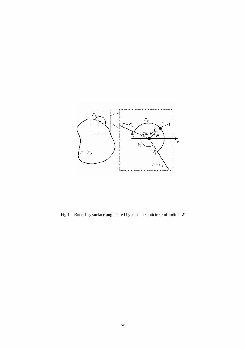
Fig.1 Boundary surface augmented by a small semicircle of radius ε

Apart from the above approach, the value of the free term is derived as follows. Consider a small

semicircle of radius ε on the boundary as depicted in Fig.1. The source point i is assumed to be

at the center of this semicircle and afterwards the radius ε is reduced to zero [2]. In this case one

should start with the boundary integral equation for an internal point

* * * ( , ) ( , ) *( , )

,,

l m l ml m

i l m il m

d dr n r n r n r n


∂ ∂ ∂ ∂ − − Γ = − − Γ ∂ ∂ ∂ ∂ ∑∫ ∫ (49)

not with Eq.(46). Each of the boundary integrals of the LHS is divided into two parts, i.e.,

* * *

d d dr n r n r nε ε

ψ ψ ψ ψ ψ ψΓ Γ Γ−Γ

∂ ∂ ∂Γ = Γ + Γ∂ ∂ ∂∫ ∫ ∫ (50a)

and

* * *

d d dr n r n r nε ε

ψ ψ ψ ψ ψ ψΓ Γ Γ−Γ

∂ ∂ ∂Γ = Γ + Γ∂ ∂ ∂∫ ∫ ∫ . (50b)

The limit of the integral along the small semicircle in Eq.(50a) can be reduced as

2

1

2

1

* *

0 0

0

lim lim

1lim log log8 0,2 2

i

i

d dr n n r

a a aa dn r

ε

θ

ε θε ε

θ

θε

ψψ ψ ψ ε θ

ψ ε θπ ε π π

Γ→ →

→

∂∂ Γ =∂ ∂

∂ → + − = ∂

∫ ∫

∫

15

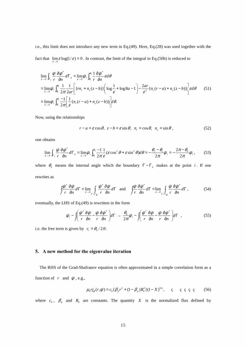
i.e., this limit does not introduce any new term in Eq.(49). Here, Eq.(28) was used together with the

fact that 0

lim log(1/ ) 0ε

ε ε→

= . In contrast, the limit of the integral in Eq.(50b) is reduced to

2

1

2

1

2

1

* *

0 0

20

0

1lim lim

1 1 1 2lim ( ) log log8 1 ( ) ( )2 2

1 1lim ( ) ( ) .2

i

i r z r z

i r z

d dr n r n

arrn n z b a n r a n z b dar

n r a n z b d

ε

θ

ε θε ε

θ

θε

θ

θε

ψ ψ ψψ ε θ

ψ ε θπ ε ε

ψ θπ ε

Γ→ →

→

→

∂ ∂Γ =∂ ∂

= + − + − − − + − − = − + −

∫ ∫

∫

∫

(51)

Now, using the relationships

cos , sin , cos , sinr zr a z b n nε θ ε θ θ θ− = − = = = , (52)

one obtains

2

1

*2 2 02 1

0 0

21 1lim lim ( cos sin )2 2 2i i id d

r nε

θ

ε θε ε

π θθ θψ ψ ψ ε θ ε θ θ ψ ψπ ε π πΓ→ →

−−∂ −Γ = + = − = −∂∫ ∫ , (53)

where 0θ means the internal angle which the boundary εΓ − Γ makes at the point i . If one

rewrites as

* *

0limd d

r n r nεε

ψ ψ ψ ψ→

Γ Γ−Γ

∂ ∂Γ = Γ∂ ∂∫ ∫ and

* *

0limd d

r n r nεε

ψ ψ ψ ψ→

Γ Γ−Γ

∂ ∂Γ = Γ∂ ∂∫ ∫ , (54)

eventually, the LHS of Eq.(49) is rewritten in the form

* * * *0

2i id dr n r n r n r n

θψ ψ ψ ψ ψ ψ ψ ψψ ψπΓ Γ

∂ ∂ ∂ ∂− − Γ → − − Γ ∂ ∂ ∂ ∂ ∫ ∫ , (55)

i.e. the free term is given by 0 / 2ic θ π= .

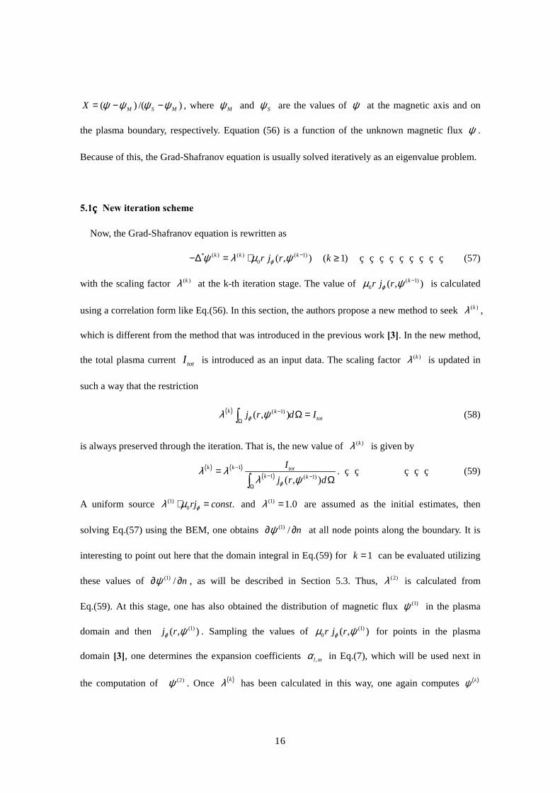
5. A new method for the eigenvalue iteration

The RHS of the Grad-Shafranov equation is often approximated in a simple correlation form as a

function of r and ψ , e.g.,

2 2 0.60 0 0( , ) (1 ) (1 )p prj r c r R Xϕµ ψ β β= + − − , (56)

where 0c , pβ and 0R are constants. The quantity X is the normalized flux defined by

16

( ) /( )M S MX ψ ψ ψ ψ= − − , where Mψ and Sψ are the values of ψ at the magnetic axis and on

the plasma boundary, respectively. Equation (56) is a function of the unknown magnetic flux ψ .

Because of this, the Grad-Shafranov equation is usually solved iteratively as an eigenvalue problem.

5.1 New iteration scheme

Now, the Grad-Shafranov equation is rewritten as

* ( ) ( ) ( 1)0 ( , ) ( 1)k k kr j r kϕψ λ µ ψ −−∆ = ⋅ ≥ (57)

with the scaling factor ( )kλ at the k-th iteration stage. The value of ( 1)0 ( , )kr j rϕµ ψ − is calculated

using a correlation form like Eq.(56). In this section, the authors propose a new method to seek ( )kλ ,

which is different from the method that was introduced in the previous work [3]. In the new method,

the total plasma current totI is introduced as an input data. The scaling factor ( )kλ is updated in

such a way that the restriction

( ) ( 1)( , )k ktotj r d Iϕλ ψ −

ΩΩ =∫ (58)

is always preserved through the iteration. That is, the new value of ( )kλ is given by

( ) ( )( )

11 ( 1)( , )

k k totk k

Ij r dϕ

λ λλ ψ

−− −

Ω

=Ω∫

. (59)

A uniform source (1)0 .rj constϕλ µ⋅ = and (1) 1.0λ = are assumed as the initial estimates, then

solving Eq.(57) using the BEM, one obtains (1) / nψ∂ ∂ at all node points along the boundary. It is

interesting to point out here that the domain integral in Eq.(59) for 1k = can be evaluated utilizing

these values of (1) / nψ∂ ∂ , as will be described in Section 5.3. Thus, (2)λ is calculated from

Eq.(59). At this stage, one has also obtained the distribution of magnetic flux (1)ψ in the plasma

domain and then (1)( , )j rϕ ψ . Sampling the values of (1)0 ( , )r j rϕµ ψ for points in the plasma

domain [3], one determines the expansion coefficients ,l mα in Eq.(7), which will be used next in

the computation of (2)ψ . Once ( )kλ has been calculated in this way, one again computes ( )kψ

17

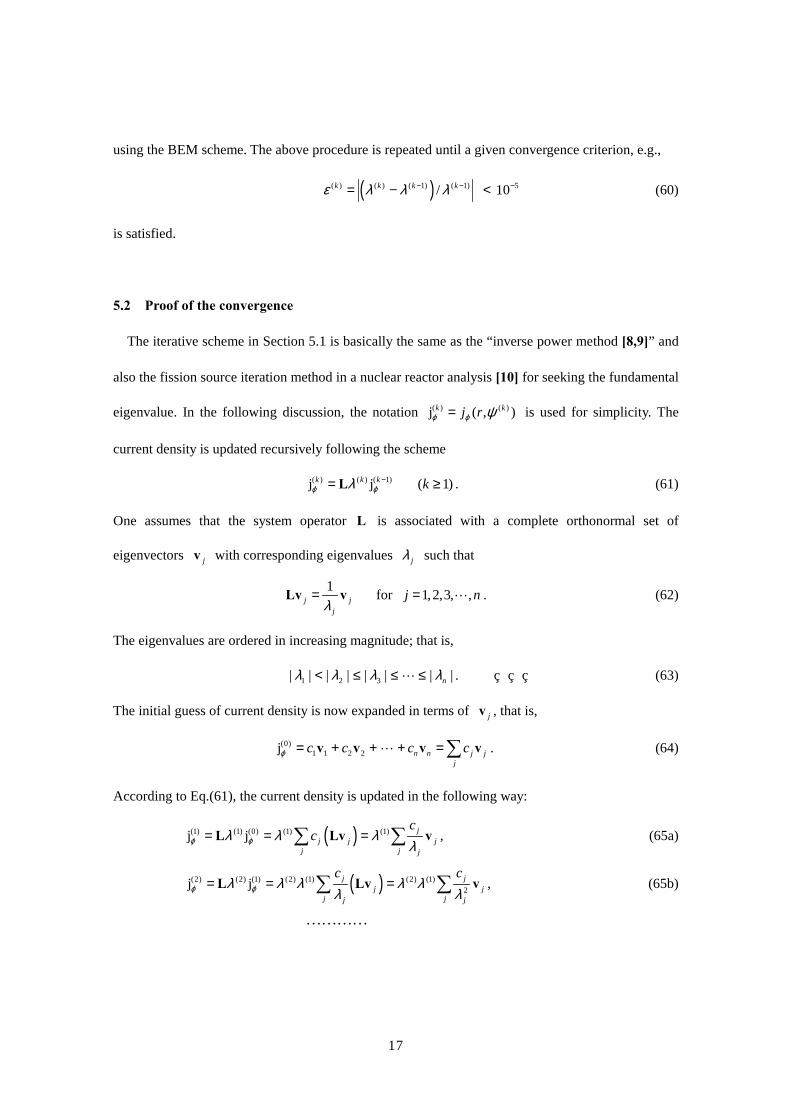
using the BEM scheme. The above procedure is repeated until a given convergence criterion, e.g.,

( )( ) ( ) ( 1) ( 1) 5/ 10k k k kε λ λ λ− − −= − < (60)

is satisfied.

5.2 Proof of the convergence

The iterative scheme in Section 5.1 is basically the same as the “inverse power method [8,9]” and

also the fission source iteration method in a nuclear reactor analysis [10] for seeking the fundamental

eigenvalue. In the following discussion, the notation ( ) ( )j ( , )k kj rϕ ϕ ψ= is used for simplicity. The

current density is updated recursively following the scheme

( ) ( ) ( 1)j j ( 1)k k k kϕ ϕλ −= ≥L . (61)

One assumes that the system operator L is associated with a complete orthonormal set of

eigenvectors jv with corresponding eigenvalues jλ such that

1j j

jλ=Lv v for 1,2,3, ,j n= ! . (62)

The eigenvalues are ordered in increasing magnitude; that is,

1 2 3| | | | | | | |nλ λ λ λ< ≤ ≤ ≤! . (63)

The initial guess of current density is now expanded in terms of jv , that is,

(0)1 1 2 2j n n j j

jc c c cϕ = + + + =∑v v v v! . (64)

According to Eq.(61), the current density is updated in the following way:

( )(1) (1) (0) (1) (1)j j ,jj j j

j j j

ccϕ ϕλ λ λ

λ= = =∑ ∑L Lv v (65a)

( )(2) (2) (1) (2) (1) (2) (1)2j j ,j j

j jj jj j

c cϕ ϕλ λ λ λ λ

λ λ= = =∑ ∑L Lv v (65b)

!!!!

18

( 2) ( 2) ( 3)

22( 2) ( 3) (2) (1)1 1

1 1 2 221 2

j j

,

k k k

kkk k

n nkn

c c c

ϕ ϕλ

λ λλ λ λ λλ λ λ

− − −

−−− −

−

=

= + + +

L

v v v! ! (66a)

( 1) ( 1) ( 2)

11( 1) ( 2) (2) (1)1 1

1 1 2 211 2

j j

.

k k k

kkk k

n nkn

c c c

ϕ ϕλ

λ λλ λ λ λλ λ λ

− − −

−−− −

−

=

= + + +

L

v v v! ! (66b)

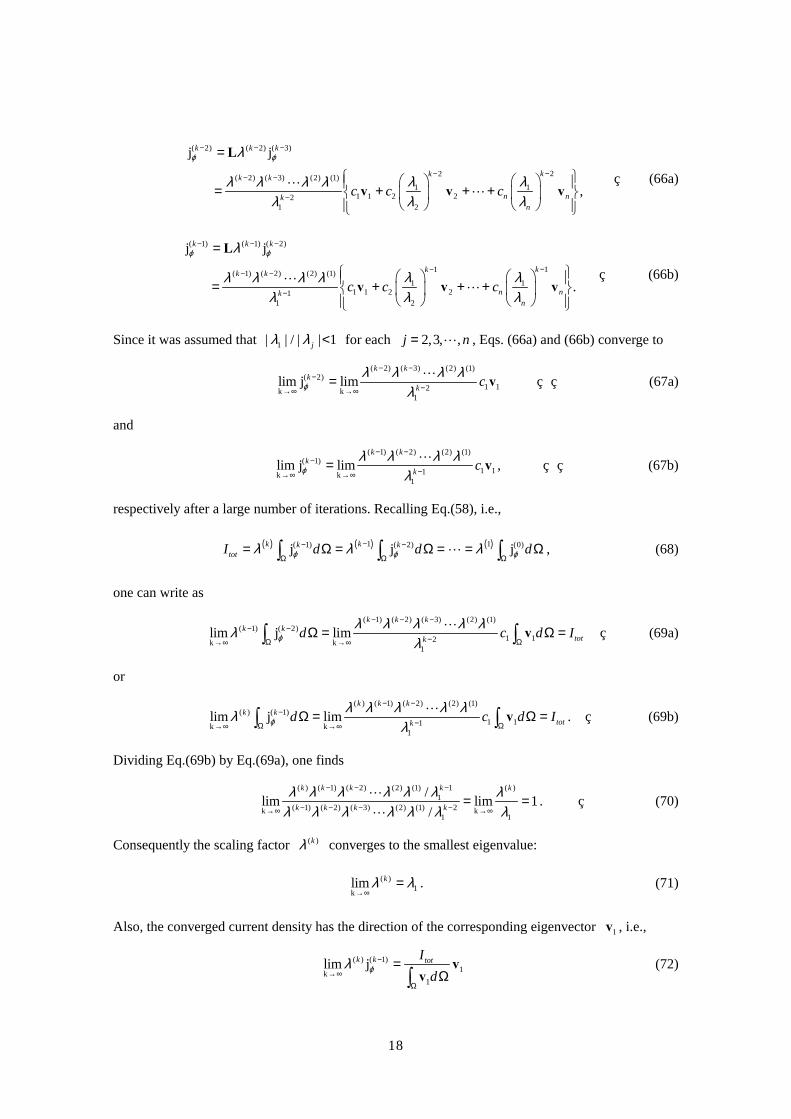
Since it was assumed that 1| | / | | 1jλ λ < for each 2,3, ,j n= ! , Eqs. (66a) and (66b) converge to

( 2) ( 3) (2) (1)( 2)

1 12k k1

lim j limk k

kk cϕ

λ λ λ λλ

− −−

−→∞ →∞= v! (67a)

and

( 1) ( 2) (2) (1)( 1)

1 11k k1

lim j limk k

kk cϕ

λ λ λ λλ

− −−

−→∞ →∞= v! , (67b)

respectively after a large number of iterations. Recalling Eq.(58), i.e.,

( ) ( ) ( )1 1( 1) ( 2) (0)j j jk kk ktotI d d dϕ ϕ ϕλ λ λ−− −

Ω Ω Ω= Ω = Ω = = Ω∫ ∫ ∫! , (68)

one can write as

( 1) ( 2) ( 3) (2) (1)( 1) ( 2)

1 12k k1

lim j limk k k

k ktotkd c d Iϕ

λ λ λ λ λλλ

− − −− −

−Ω Ω→∞ →∞Ω = Ω =∫ ∫ v! (69a)

or

( ) ( 1) ( 2) (2) (1)( ) ( 1)

1 11k k1

lim j limk k k

k ktotkd c d Iϕ

λ λ λ λ λλλ

− −−

−Ω Ω→∞ →∞Ω = Ω =∫ ∫ v! . (69b)

Dividing Eq.(69b) by Eq.(69a), one finds

( ) ( 1) ( 2) (2) (1) 1 ( )1

( 1) ( 2) ( 3) (2) (1) 2k k1 1

/lim lim 1/

k k k k k

k k k k

λ λ λ λ λ λ λλ λ λ λ λ λ λ

− − −

− − − −→∞ →∞= =!

!. (70)

Consequently the scaling factor ( )kλ converges to the smallest eigenvalue:

( )1k

lim kλ λ→∞

= . (71)

Also, the converged current density has the direction of the corresponding eigenvector 1v , i.e.,

( ) ( 1)1k

1

lim jk k totIdϕλ −

→∞Ω

=Ω∫

vv

(72)

19

due to the relationship ( ) ( 1) ( 2) (2) (1)

11k1 1

limk k k

totk

Icd

λ λ λ λ λλ

− −

−→∞Ω

=Ω∫ v

! . (73)

5.3 New boundary expression of the total current

Corresponding to the given total current totI , one needs to evaluate the domain integral in Eq.(59)

through the iteration. Itagaki et al. [3,4] transformed the polynomial-expanded domain integral

( )( ) ( ), 0

,( , ) /k k l m

l ml m

j r d r dϕ ψ α ξ η µΩ Ω

Ω Ω∑∫ ∫" (74)

into a boundary integral by using the particular solution ( , )l mφ that satisfies 2 ( , )l m l mφ ξ η∇ = and

applying the Gauss theorem. The new technique proposed here is more elegant in the sense that it

does not rely on the polynomial expansion.

According to Ampere’s law, the total current totI flowing through the area enclosed by a closed

path can be determined using the line integral of the poloidal field pB around the closed path, as

0

1tot pI B ds

µ= ∫# . (75)

As the poloidal field is given by (1/ )( / )pB r nψ= ∂ ∂ , the domain integral in Eq.(59) can be

transformed into a circular integral along the plasma boundary, i,e.,

( )( 1) ( 1)

0

1 1( , )k

k kj r d dr nϕ

ψλ ψµ

− −

Ω Γ

∂Ω = Γ∂∫ ∫ . (76)

The computation of this circular integral is quite simple, and does not require any complicated

numerical operation arising from polynomial expansion.

6. Numerical examples

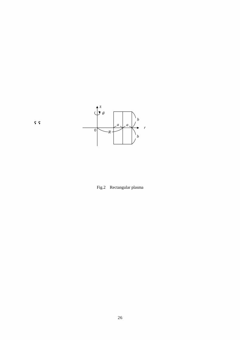
6.1 Rectangular plasma

Assume a hypothetical rectangular plasma as shown in Fig.2. The boundary condition 0ψ = is

20

imposed along each side of the rectangle. In this case, an analytic solution exists [3] for the equation

with a monomial l mr z source term

2

2

1 l mr r zr r r z

ψ ∂ ∂ ∂ − + = ∂ ∂ ∂ ( 0, 0)l m≥ ≥ . (77)

One assumes here the sizes: 0.5[m], 0.5[m],a b= = and 1.0[m]R = .

Fig.2 Rectangular plasma

Boundary element analyses were performed using the constant and the discontinuous quadratic

boundary elements. In the constant element calculation, each side of the rectangle was equally

divided, and a total of 72 elements, i.e., 72 node points, were employed. In the discontinuous

quadratic element calculation, a total of 24 boundary elements were taken in such a way that the

number of node points is equal to that used in the constant element calculation (=72). Comparisons

were made between the analytic and the boundary element solutions for all combinations of integers

l and m in the range 0 8l m≤ + ≤ .

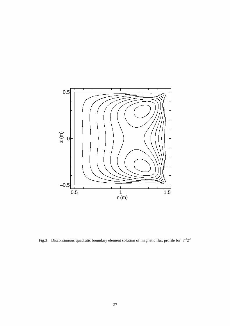
As an example, Fig.3 shows the contour map of the discontinuous quadratic boundary element

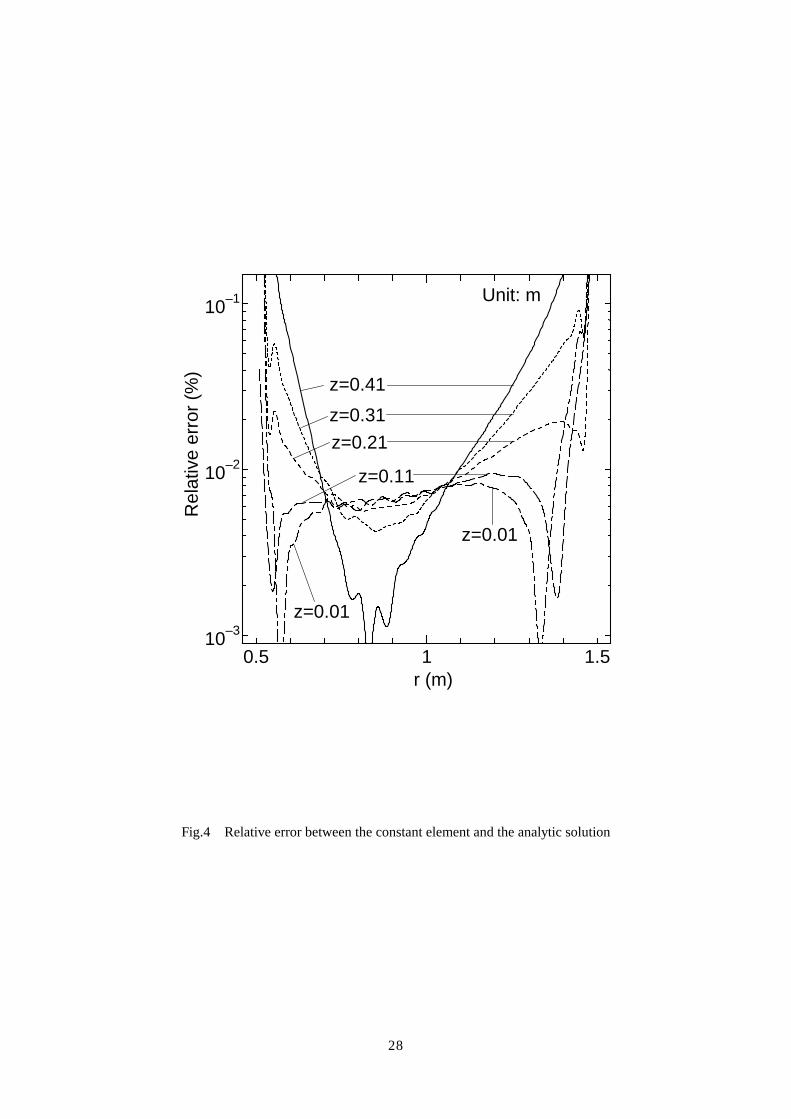
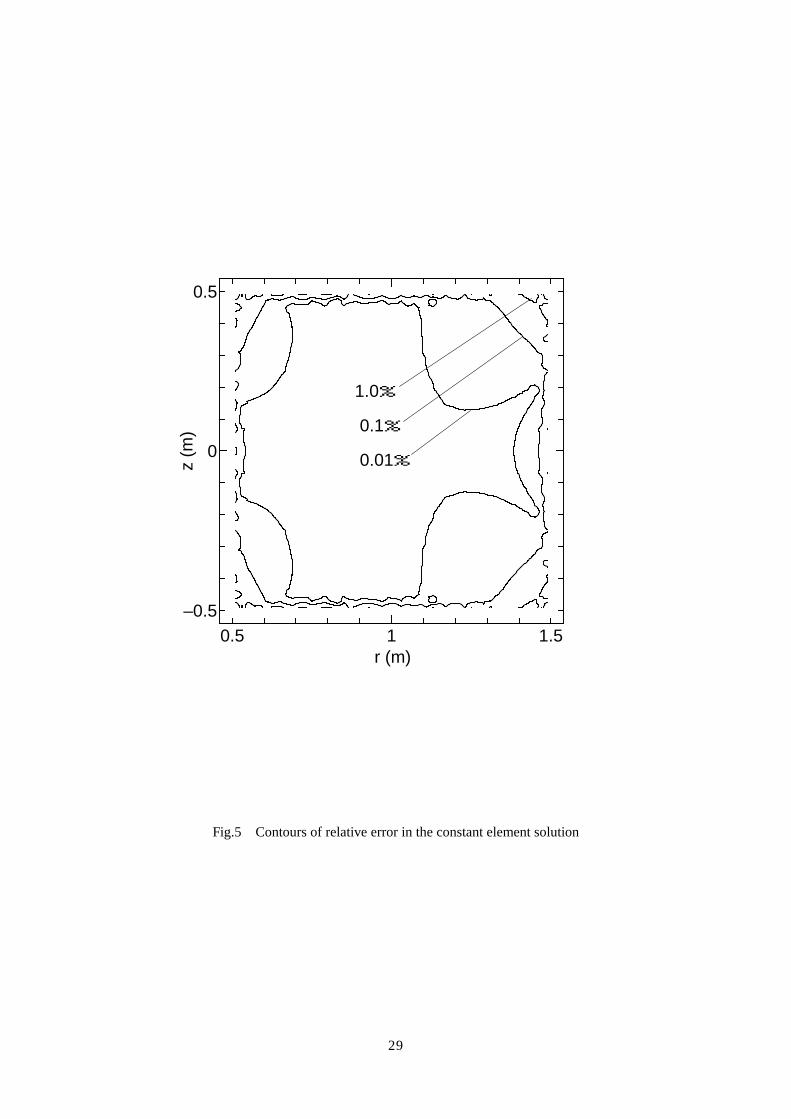
solution of ψ for a monomial source 3 2r z . As for the constant element calculation for the same

problem, the relative error from the analytic solution, defined by ((BEM-analytic)/analytic) 100× , is

illustrated in Fig.4 and Fig.5. In Fig.4, the relative deviations are plotted along the lines z=0.01m,

0.11m, 0.21m, 0.31m and 0.41m. Figure 5 is a contour map. The relative error in the discontinuous

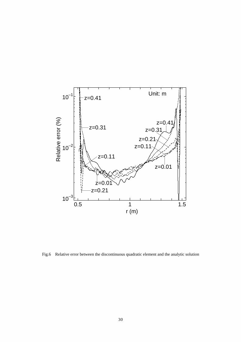
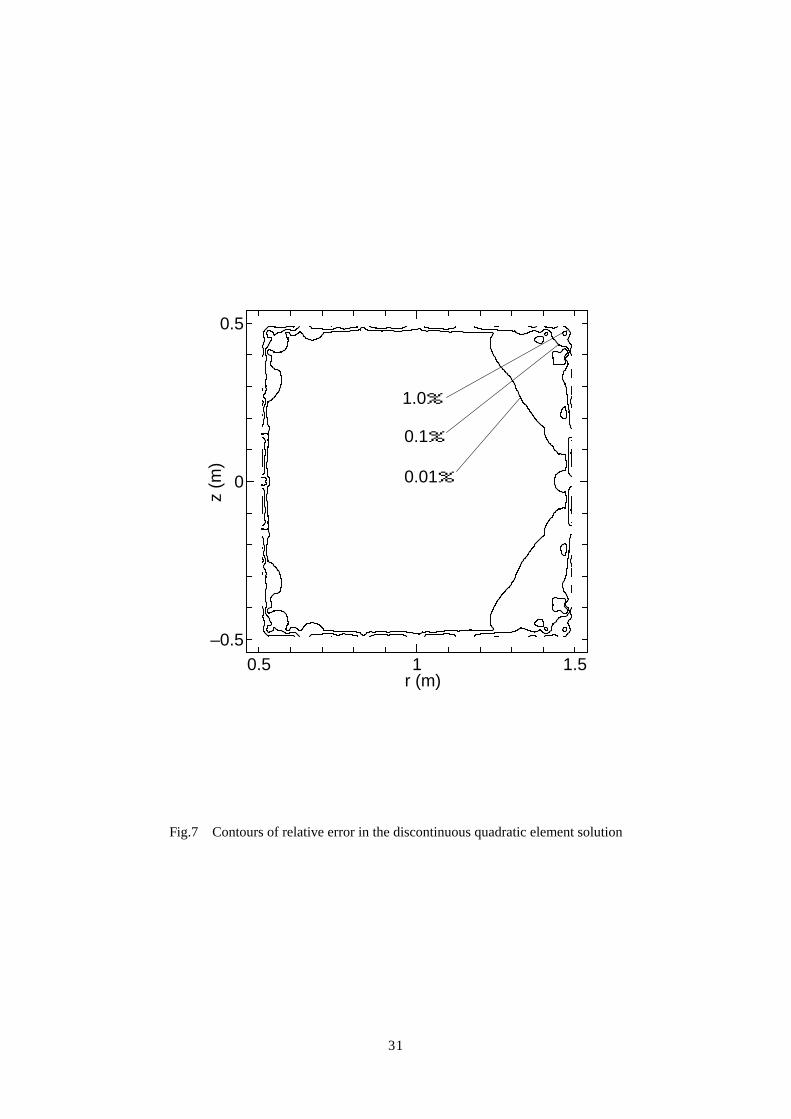
quadratic element calculation is also shown in Fig.6 and Fig.7. The region where the relative error is

less than 0.01% in the discontinuous quadratic element calculation is much larger than that in the

constant element calculation in spite of the same number of node points being adopted. An error

larger than 1% is found near the edges and corners in the both calculations; however, the absolute

values of ψ are extremely small in these places. Almost the same level of accuracy was also

demonstrated for each of other combinations of l and m .

21

Fig.3 Discontinuous quadratic boundary element solution of magnetic flux profile for 3 2r z

Fig.4 Relative error between the constant element and the analytic solution

Fig.5 Contours of relative error in the constant element solution

Fig.6 Relative error between the discontinuous quadratic element and the analytic solution

Fig.7 Contours of relative error in the discontinuous quadratic element solution

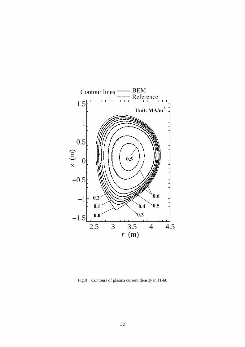
6.2 Tokamak geometry

One here considers the problem of modelling the JT-60 tokamak-device. By courtesy of Japan

Atomic Energy Research Institute (JAERI), the reference data of plasma boundary, distributions of

plasma current density and magnetic flux were first provided. These had been obtained from an

analysis using a reliable equilibrium code, SELENE, which is based on the finite element method

[11]. An equilibrium computation was made based on a “hollow” current profile parametrization that

has the form

2 20 0 0

2 (1 ) (1 3 4 )( , ) p prj c r R X Xrϕµ β βψ = + − + − . (78)

Here, ( ) /( )M S MX ψ ψ ψ ψ= − − in which Mψ and Sψ are the values of ψ on the magnetic axis

and on the boundary, while pβ (= 0.70199) and 0R (=3.39927 m) denote the poloidal beta and the

characteristic major radius, respectively.

This problem was again analyzed using the BEM as a fixed boundary problem. Only the boundary

shape among the SELENE computing results was transferred to the BEM computation as input data.

The boundary condition 0ψ = was imposed at each nodal point along the boundary. The same

current profile parametrization shown above was again assumed. The complete polynomial of the

8-th order was adopted to approximate the 0rjϕµ distribution, and hence the polynomial consists of

a total of 45 terms. To determine the polynomial expansion coefficients, a total of 1758 sampling

points was automatically generated within the domain. The plasma boundary is approximated by a

22

total of 57 discontinuous quadratic boundary elements, i.e., a total of 171 node points was employed.

A total of 7 iterations was required in the BEM analysis when the eigenvalue deviation defined by

Eq.(60) was reduced to less than 510− . The profile of magnetic flux function thus obtained from the

discontinuous quadratic BEM calculation is compared with the SELENE calculation results, as

shown in Fig.8. The plasma current profiles are also compared in Fig.9. In each figure, the solid

lines show the BEM solutions, while the dashed lines denote the reference results obtained using the

SELENE code. The BEM results show good agreement with the reference data, and this

demonstrates the validity of the present boundary-only integral formulation, especially of the

polynomial expansion approximation of 0rjϕµ .

Fig.8 Contours of plasma current density in JT-60

Fig.9 Contours of magnetic flux in JT-60

7. Conclusions

The singularity of the fundamental solution and the properties of singular integrals peculiar to the

Grad-Shafranov equation have been carefully investigated. For example, the value of ˆiiH given in

Section 3 is not zero even for the straight-line elements unlike the same quantity derived from the

Laplace equation. It has been confirmed that the fundamental solution, its derivative, and all derived

boundary integrals represent not a strong but a ‘weak’ singularity at the most. These weak singular

integrals can be managed with the subtraction scheme shown in Eqs.(29a), (29b), (45a) and (45b),

and then by using the standard and the logarithmic Gaussian quadrature rules or analytic integrals.

On the basis of the above facts, the discontinuous quadratic boundary elements have been

introduced to give more accurate solutions than those obtained by using constant elements.

The new eigenvalue calculation scheme based on the total current estimated according to

23

Ampere’s law has been proposed and the test calculation demonstrates its validity.

Acknowledgements

This paper includes the achievement of ‘Fiscal 2005 Research Cooperation with JAERI on

Experiments and Analyses Using the Critical Plasma Test Equipment JT-60’. The authors wish to

express their gratitude to Dr. K. Kurihara of JAERI for his valuable and helpful comments on this

work. Further, he kindly provided them with the reference tokamak plasma data used in the

numerical demonstration in section 6.

References

(1) Wesson, J, “Tokamaks (Second edition)”, The Oxford Engineering Series 48, Clarendon Press,

Oxford (1997).

(2) Brebbia, C.A., “The Boundary Element Method for Engineers”, Pentech Press, London (1978)

(3) Itagaki, M., Kamisawada, J., Oikawa, S., “Boundary- only integral equation approach based on

polynomial expansion of plasma current profile to solve the Grad-Shafranov equation”, Nuclear

Fusion, 44, 427-437 (2004).

(4) Itagaki, M., Yamaguchi, S., Fukunaga, T., “Boundary integral equation approach based on a

polynomial expansion of the current distribution to reconstruct the current density profile in

tokamak plasmas,” Nuclear Fusion, 45, 153-162 (2005).

(5) Brebbia, C.A., Dominguez, J., “Boundary Elements – An Introductory Course”, Computational

Mechanics Publications, Southampton (1992).

(6) Abramowitz, M., Stegun, I.A.: “Handbook of Mathematical Functions”, Dover Publications,

New York (1965).

24

(7) Stroud, A.H., Secrest, D., “Gaussian Quadrature Formulas”, Prentice-Hall, New York (1966).

(8) Watkins, D. S., “Fundamentals of Matrix Computations”, John Wiley & Sons, New York (1991).

(9) Mathews, J. H., Fink, K. D., “Numerical Methods Using MATLAB, Fourth Edition”, Pearson

Prentice Hall, Upper Saddle River, New Jersey (2004).

(10) Itagaki, M., Sahashi, N., “Three-dimensional Multiple Reciprocity Boundary Element Method

for Solving Neutron Diffusion Critical Eigenvalue Computations”, J. Nucl. Sci. Tech., 33[2],

101-109 (1996)

(11) Takeda, T., Tsunematsu, T., “A Numerical Code SELENE To Calculate Axisymmetric Toroidal

MHD Equilibria”, JAERI-M 8042, Japan Atomic Energy Research Institute (1978).

List of Figures










25


i

εΓ Γ−

εΓεΓ

εΓ Γ−

εΓ Γ−

εθ

0θ

( ),r zx

( , )a bξ

1θ

2θ

r

26

bθ

r0 R

aa

b

z


27


0.5 1 1.5–0.5

0

0.5

r (m)

z (m

)

28


0.5 1 1.510–3

10–2

10–1

Rel

ativ

e er

ror (

%)

r (m)

z=0.41z=0.31z=0.21

z=0.11

z=0.01

z=0.01

Unit: m

29


0.5 1 1.5–0.5

0

0.5

r (m)

z (m

)

0.01％

1.0％

0.1％

30


0.5 1 1.510–3

10–2

10–1

Rel

ativ

e er

ror (

%)

r (m)

z=0.31

Unit: mz=0.41

z=0.01

z=0.41z=0.31

z=0.21z=0.11

z=0.01z=0.21

z=0.11

31


0.5 1 1.5–0.5

0

0.5

r (m)

z (m

)

1.0％

0.1％

0.01％

32


2.5 3 3.5 4 4.5–1.5

–1

–0.5

0

0.5

1

1.5

r (m)

z (m

)

Contour lines BEMReference

0.0

0.10.2

0.30.4 0.5

0.6

0.5

Unit: MA/m2

33


2.5 3 3.5 4 4.5–1.5

–1

–0.5

0

0.5

1

1.5

r (m)

z (m

)

Contour lines BEMReference

X–point

Unit: Wb

0.10.2 0.0

0.10.20.3

0.4

0.5

Boundary element modelling to solve the Grad … · Boundary element modelling to solve the...

Documents

Transcript of Boundary element modelling to solve the Grad … · Boundary element modelling to solve the...