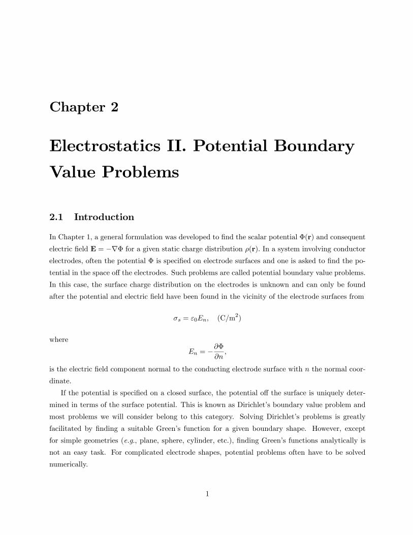
Chapter 2

Electrostatics II. Potential Boundary

Value Problems

2.1 Introduction

In Chapter 1, a general formulation was developed to find the scalar potential Φ(r) and consequent

electric field E = −∇Φ for a given static charge distribution ρ(r). In a system involving conductor

electrodes, often the potential Φ is specified on electrode surfaces and one is asked to find the po-

tential in the space off the electrodes. Such problems are called potential boundary value problems.

In this case, the surface charge distribution on the electrodes is unknown and can only be found

after the potential and electric field have been found in the vicinity of the electrode surfaces from

σs = ε0En, (C/m2)

where

En = −∂Φ

∂n,

is the electric field component normal to the conducting electrode surface with n the normal coor-

dinate.

If the potential is specified on a closed surface, the potential off the surface is uniquely deter-

mined in terms of the surface potential. This is known as Dirichlet’s boundary value problem and

most problems we will consider belong to this category. Solving Dirichlet’s problems is greatly

facilitated by finding a suitable Green’s function for a given boundary shape. However, except

for simple geometries (e.g., plane, sphere, cylinder, etc.), finding Green’s functions analytically is

not an easy task. For complicated electrode shapes, potential problems often have to be solved

numerically.

1

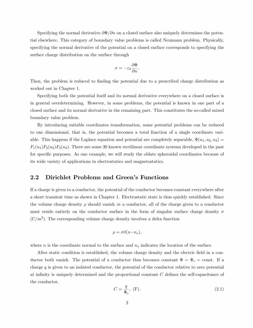
Specifying the normal derivative ∂Φ/∂n on a closed surface also uniquely determines the poten-

tial elsewhere. This category of boundary value problems is called Neumann problem. Physically,

specifying the normal derivative of the potential on a closed surface corresponds to specifying the

surface charge distribution on the surface through

σ = −ε0∂Φ

∂n.

Then, the problem is reduced to finding the potential due to a prescribed charge distribution as

worked out in Chapter 1.

Specifying both the potential itself and its normal derivative everywhere on a closed surface is

in general overdetermining. However, in some problems, the potential is known in one part of a

closed surface and its normal derivative in the remaining part. This constitutes the so-called mixed

boundary value problem.

By introducing suitable coordinates transformation, some potential problems can be reduced

to one dimensional, that is, the potential becomes a total function of a single coordinate vari-

able. This happens if the Laplace equation and potential are completely separable, Φ(u1, u2, u3) =

F1(u1)F2(u2)F3(u3). There are some 30 known rectilinear coordinate systems developed in the past

for specific purposes. As one example, we will study the oblate spheroidal coordinates because of

its wide variety of applications in electrostatics and magnetostatics.

2.2 Dirichlet Problems and Green’s Functions

If a charge is given to a conductor, the potential of the conductor becomes constant everywhere after

a short transient time as shown in Chapter 1. Electrostatic state is thus quickly established. Since

the volume charge density ρ should vanish in a conductor, all of the charge given to a conductor

must reside entirely on the conductor surface in the form of singular surface charge density σ

(C/m2). The corresponding volume charge density involves a delta function

ρ = σδ(n−ns),

where n is the coordinate normal to the surface and ns indicates the location of the surface.

After static condition is established, the volume charge density and the electric field in a con-

ductor both vanish. The potential of a conductor thus becomes constant Φ = Φc = const. If a

charge q is given to an isolated conductor, the potential of the conductor relative to zero potential

at infinity is uniquely determined and the proportional constant C defines the self-capacitance of

the conductor,

C =q

Φc, (F). (2.1)

2

Let us consider a trivial case, a conducting sphere of radius a carrying a charge q. The potential

outside the sphere is given by

Φ(r) =q

4πε0

1

r, r ≥ a. (2.2)

The sphere potential is

Φs =q

4πε0a, (2.3)

which determines the self-capacitance of the sphere,

C = 4πε0a, (F). (2.4)

The outer potential Φ(r) can be written in the form

Φ(r) =a

rΦs, r > a, (2.5)

which indicates that the potential is uniquely determined if the sphere potential Φs is known. In

general, if the potential is specified everywhere on a closed surface, the potential elsewhere off

the surface is uniquely determined in terms of the surface potential Φs(rs) where rs denotes the

coordinates on the closed surface. This is known as Dirichlet’s theorem and finding a potential for

given boundary potential distribution on a closed surface is called Dirichlet’s problem.

The same problem can also be solved in terms of the electric field on the sphere surface,

Er =1

4πε0

q

a2, (2.6)

which can be replaced with a surface charge,

σ = ε0Er =q

4πa2, (C/m2). (2.7)

The potential due to the uniform surface charge is

Φ(r) =1

4πε0

∮σ

|r− r′|dS

=σ

4πε02πa2

∫ π

0

1√r2 + a2 − 2ar cos θ

sin θdθ

=q

4πε0r, (r > a) (2.8)

where θ is measured from the direction of r. (This is allowed because of symmetry. For r < a, the

integral yields

Φ(r) =q

4πε0a= const., (r < a, interior)

3

which is also an expected result.) Since

Er = −∂Φ

∂r=∂Φ

∂n, (2.9)

where n is the normal coordinate on the surface directed away from the volume of interest, the

potential can be rewritten as

Φ(r) =1

4π

∮S

1

|r− r′|∂Φ

∂ndS′. (2.10)

As this simple example indicates, potential boundary value problems can be solved in terms of

either the surface potential Φs or its normal derivative, ∂Φ/∂n. The latter method may be regarded

as a boundary value problem for the electric field.

Let us revisit the potential due to a prescribed charge distribution,

Φ(r) =1

4πε0

∫ρ(r′)

|r− r′|dV′. (2.11)

The potential can be understood as a convolution between the charge density distribution ρ(r) and

the function

G(r, r′) =1

4π

1

|r− r′| , (2.12)

which is the particular solution to the singular Poisson’s equation

∇2G = −δ(r− r′), (2.13)

subject to the boundary condition that G vanish at infinity. The function G is called Green’s

function. Physically, the Green’s function defined as a solution to the singular Poisson’s equation

is nothing but the potential due to a point charge placed at r = r′. In potential boundary value

problems, the charge density ρ(r) is unknown and one has to devise an alternative formulation

in terms of boundary potential Φs(r). It is noted that the Green’s function in Eq. (2.12) is the

particular solution to the singular Poisson’s equation and we still have freedom to add general

solutions satisfying Laplace equation,

G = Gp +Gg, (2.14)

where Gp is the particular solution and Gg is a collection of general solutions satisfying

∇2Gg = 0. (2.15)

This freedom will play an important role in constructing a Green’s function suitable for a given

boundary shape as we will see shortly. In doing so, we exploit the following theorem:

4

Theorem 1 Green’s Theorem: For arbitrary scalar functions φ and ψ, the following identity holds,∫V

(φ∇2ψ − ψ∇2φ

)dV =

∮S

(φ∇ψ − ψ∇φ) · dS. (2.16)

Proof of this theorem goes as follows. Gauss’theorem applied to the function φ∇ψ gives∫V∇ · (φ∇ψ)dV =

∮S

(φ∇ψ) · dS. (2.17)

The LHS may be expanded as∫V∇ · (φ∇ψ)dV =

∫V

(∇φ · ∇ψ + φ∇2ψ

)dV. (2.18)

Therefore, ∫V

(∇φ · ∇ψ + φ∇2ψ

)dV =

∮S

(φ∇ψ) · dS. (2.19)

Exchanging φ and ψ, ∫V

(∇ψ · ∇φ+ ψ∇2φ

)dV =

∮S

(ψ∇φ) · dS. (2.20)

Subtracting Eq. (2.20) from Eq. (2.19) yields∫V

(φ∇2ψ − ψ∇2φ

)dV =

∮S

(φ∇ψ − ψ∇φ) · dS, (2.21)

which is the desired identity.

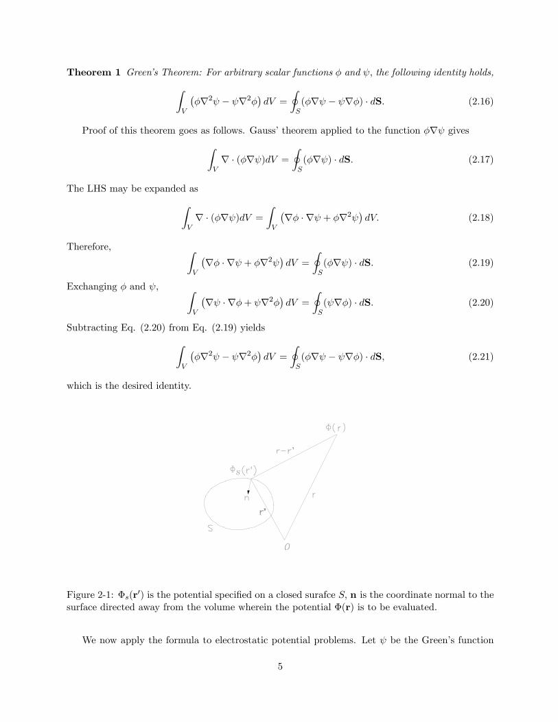
Figure 2-1: Φs(r′) is the potential specified on a closed surafce S, n is the coordinate normal to the

surface directed away from the volume wherein the potential Φ(r) is to be evaluated.

We now apply the formula to electrostatic potential problems. Let ψ be the Green’s function

5

ψ = G, satisfying

∇2G = −δ(r− r′), (2.22)

and φ = Φ be the scalar potential satisfying Poisson’s equation

∇2Φ = − ρ

ε0. (2.23)

Then, the terms in the LHS of Eq. (2.21) become∫V

Φ∇2r′GdV ′ = −∫V

Φ(r′)δ(r− r′)dV ′

= −Φ(r),

provided the coordinates r resides in the volume V where we wish to find the potential, and∫G∇2ΦdV ′ = − 1

ε0

∫Gρ(r′)dV ′. (2.24)

The RHS of Eq. (2.21) reduces to ∮S

(Φ∂G

∂n−G∂Φ

∂n

)dS, (2.25)

where Φ is the potential on the closed surface and n is the coordinate normal to the surface directed

away from the volume of interest as indicated in Fig.2-1. Therefore, the solution for the potential

Φ(r) is given by

Φ(r) =1

ε0

∫VGρ(r′)dV ′ −

∮S

(Φs∂G

∂n−G∂Φs

∂n

)dS. (2.26)

At this stage, the Green’s function is still arbitrary except it should satisfy the singular Poisson’s

equation in Eq. (2.22). The first term in the RHS allows evaluation of the potential for a given

charge distribution as we saw earlier. The surface integral involves the potential on the closed

surface Φs and its normal derivative, namely, the normal component of the electric field at the

surface.

In usual boundary value problems, the potential on a closed surface is specified as a function

of the surface coordinates. In this case, it is convenient to choose the Green’s function so that it

vanishes on the surface,

G = 0 on S.

Then the last term in Eq. (2.26) vanishes, and the solution for the potential becomes

Φ(r) =1

4πε0

∫V

ρ(r′)

|r− r′|dV′ −∮S

Φs∂G

∂ndS′, G = 0 on S. (2.27)

6

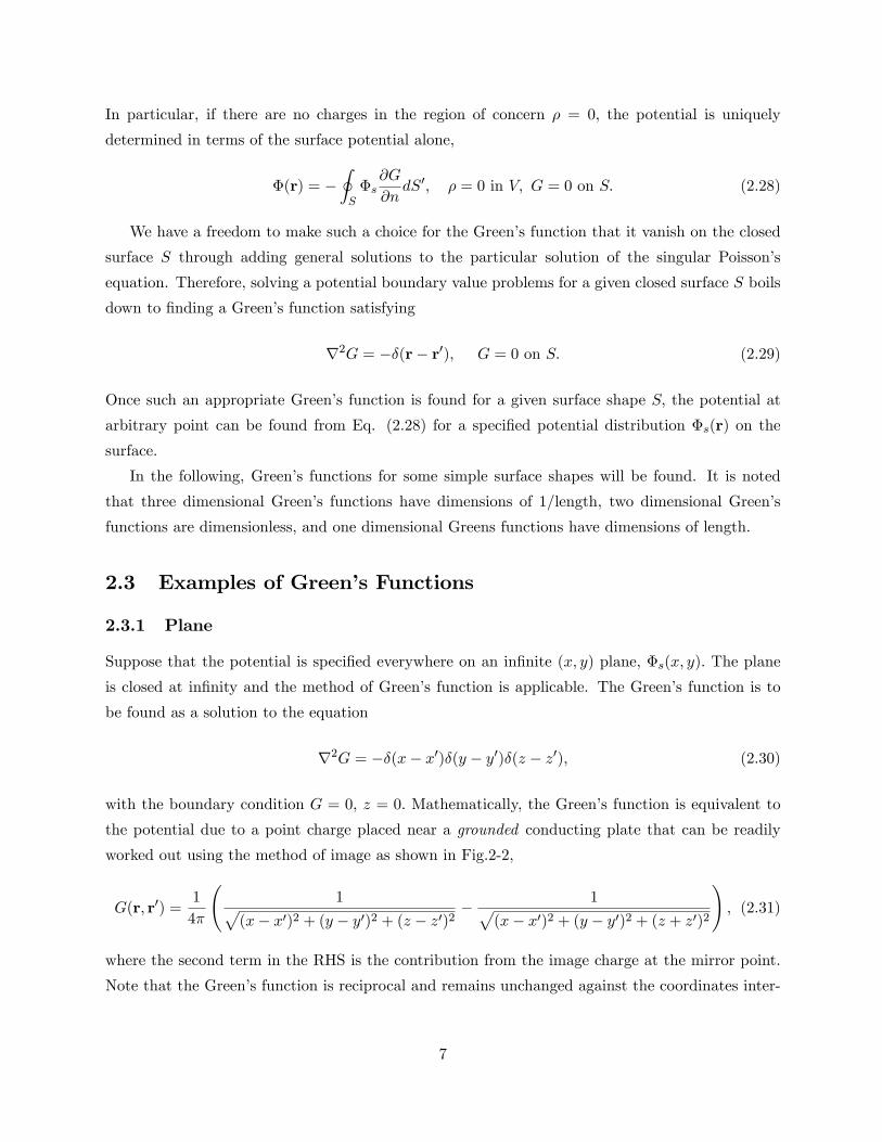
In particular, if there are no charges in the region of concern ρ = 0, the potential is uniquely

determined in terms of the surface potential alone,

Φ(r) = −∮S

Φs∂G

∂ndS′, ρ = 0 in V, G = 0 on S. (2.28)

We have a freedom to make such a choice for the Green’s function that it vanish on the closed

surface S through adding general solutions to the particular solution of the singular Poisson’s

equation. Therefore, solving a potential boundary value problems for a given closed surface S boils

down to finding a Green’s function satisfying

∇2G = −δ(r− r′), G = 0 on S. (2.29)

Once such an appropriate Green’s function is found for a given surface shape S, the potential at

arbitrary point can be found from Eq. (2.28) for a specified potential distribution Φs(r) on the

surface.

In the following, Green’s functions for some simple surface shapes will be found. It is noted

that three dimensional Green’s functions have dimensions of 1/length, two dimensional Green’s

functions are dimensionless, and one dimensional Greens functions have dimensions of length.

2.3 Examples of Green’s Functions

2.3.1 Plane

Suppose that the potential is specified everywhere on an infinite (x, y) plane, Φs(x, y). The plane

is closed at infinity and the method of Green’s function is applicable. The Green’s function is to

be found as a solution to the equation

∇2G = −δ(x− x′)δ(y − y′)δ(z − z′), (2.30)

with the boundary condition G = 0, z = 0. Mathematically, the Green’s function is equivalent to

the potential due to a point charge placed near a grounded conducting plate that can be readily

worked out using the method of image as shown in Fig.2-2,

G(r, r′) =1

4π

(1√

(x− x′)2 + (y − y′)2 + (z − z′)2− 1√

(x− x′)2 + (y − y′)2 + (z + z′)2

), (2.31)

where the second term in the RHS is the contribution from the image charge at the mirror point.

Note that the Green’s function is reciprocal and remains unchanged against the coordinates inter-

7

change,

G(r, r′) = G(r′, r).

This is expected from the fact that the delta function in the original singular Poisson’s equation is

even,

δ(r− r′) = δ(r′−r).

In the upper region z > 0,

∂G

∂n= − ∂G

∂z′

∣∣∣∣z′=0

= − 1

2π

z

[(x− x′)2 + (y − y′)2 + z2]3/2. (2.32)

Therefore, for a surface potential Φs(x′, y′) specified as a function of (x′, y′), the potential in the

region z > 0 is given by

Φ(r) =z

2π

∫ ∞−∞

dx′∫ ∞−∞

dy′Φs(x

′, y′)

[(x− x′)2 + (y − y′)2 + z2]3/2. (2.33)

Figure 2-2: Image charge −q for a large, grounded conducting plate. The potential due to q and−q vanishes at the plate.

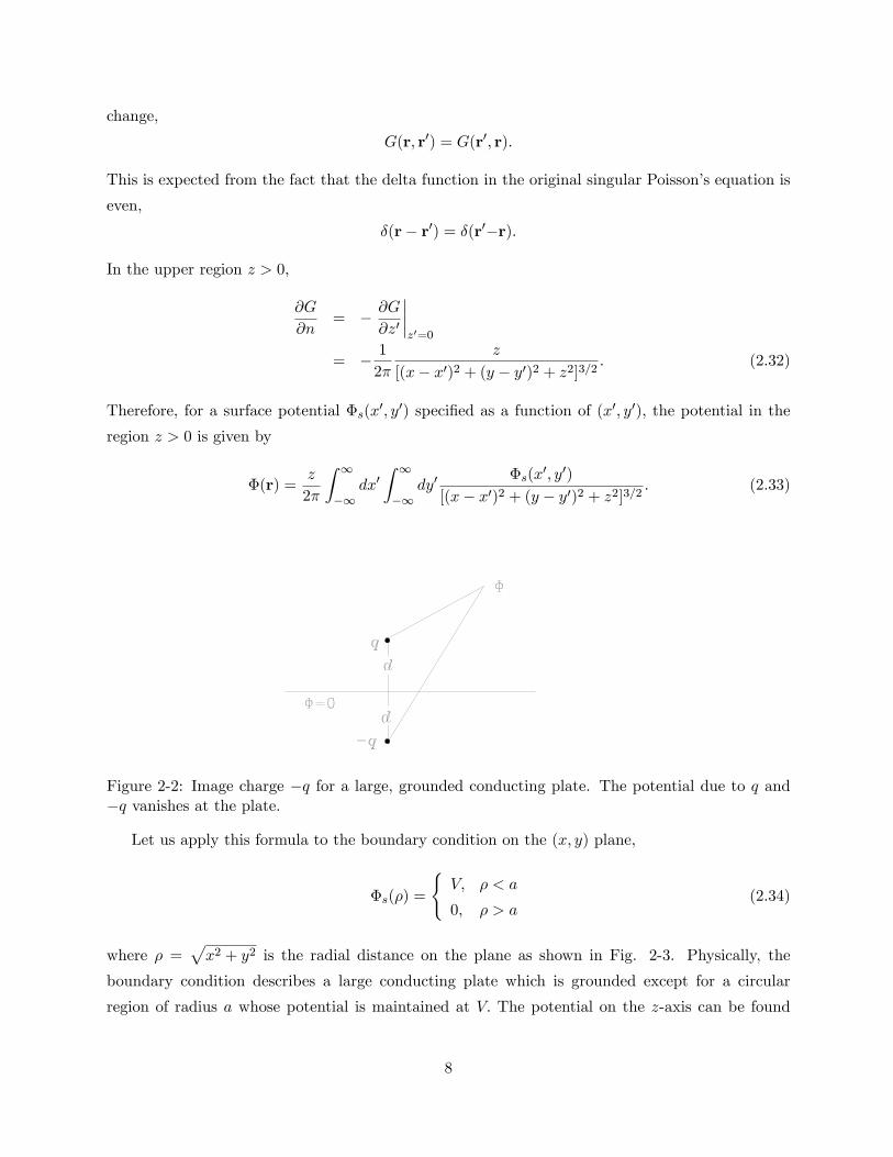
Let us apply this formula to the boundary condition on the (x, y) plane,

Φs(ρ) =

V, ρ < a

0, ρ > a(2.34)

where ρ =√x2 + y2 is the radial distance on the plane as shown in Fig. 2-3. Physically, the

boundary condition describes a large conducting plate which is grounded except for a circular

region of radius a whose potential is maintained at V. The potential on the z-axis can be found

8

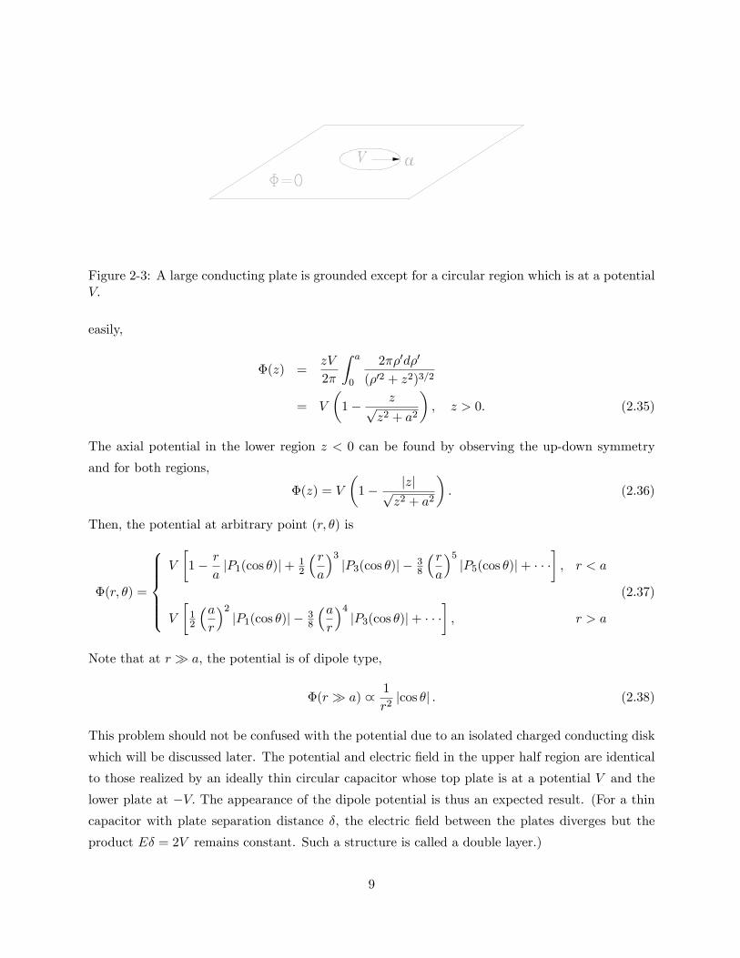
Figure 2-3: A large conducting plate is grounded except for a circular region which is at a potentialV.

easily,

Φ(z) =zV

2π

∫ a

0

2πρ′dρ′

(ρ′2 + z2)3/2

= V

(1− z√

z2 + a2

), z > 0. (2.35)

The axial potential in the lower region z < 0 can be found by observing the up-down symmetry

and for both regions,

Φ(z) = V

(1− |z|√

z2 + a2

). (2.36)

Then, the potential at arbitrary point (r, θ) is

Φ(r, θ) =

V

[1− r

a|P1(cos θ)|+ 1

2

(ra

)3|P3(cos θ)| − 3

8

(ra

)5|P5(cos θ)|+ · · ·

], r < a

V

[12

(ar

)2|P1(cos θ)| − 3

8

(ar

)4|P3(cos θ)|+ · · ·

], r > a

(2.37)

Note that at r a, the potential is of dipole type,

Φ(r a) ∝ 1

r2|cos θ| . (2.38)

This problem should not be confused with the potential due to an isolated charged conducting disk

which will be discussed later. The potential and electric field in the upper half region are identical

to those realized by an ideally thin circular capacitor whose top plate is at a potential V and the

lower plate at −V. The appearance of the dipole potential is thus an expected result. (For a thincapacitor with plate separation distance δ, the electric field between the plates diverges but the

product Eδ = 2V remains constant. Such a structure is called a double layer.)

9

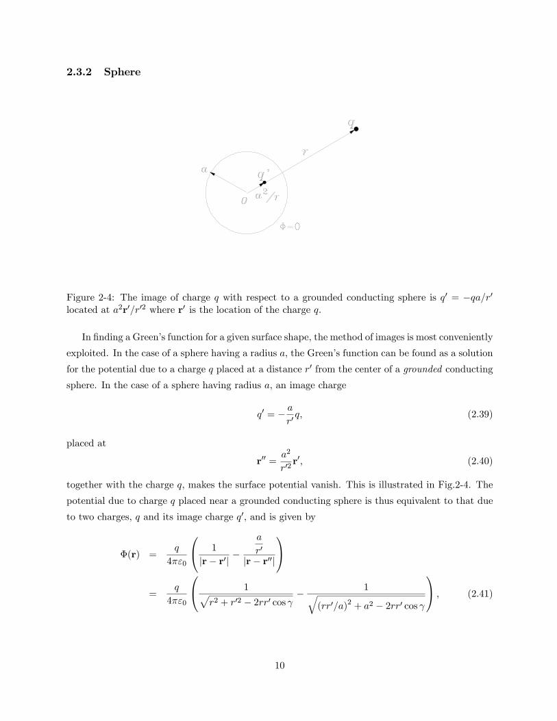
2.3.2 Sphere

Figure 2-4: The image of charge q with respect to a grounded conducting sphere is q′ = −qa/r′located at a2r′/r′2 where r′ is the location of the charge q.

In finding a Green’s function for a given surface shape, the method of images is most conveniently

exploited. In the case of a sphere having a radius a, the Green’s function can be found as a solution

for the potential due to a charge q placed at a distance r′ from the center of a grounded conducting

sphere. In the case of a sphere having radius a, an image charge

q′ = − ar′q, (2.39)

placed at

r′′ =a2

r′2r′, (2.40)

together with the charge q, makes the surface potential vanish. This is illustrated in Fig.2-4. The

potential due to charge q placed near a grounded conducting sphere is thus equivalent to that due

to two charges, q and its image charge q′, and is given by

Φ(r) =q

4πε0

1

|r− r′| −a

r′

|r− r′′|

=

q

4πε0

1√r2 + r′2 − 2rr′ cos γ

− 1√(rr′/a)2 + a2 − 2rr′ cos γ

, (2.41)

10

which readily yields the Green’s function for a sphere,

G(r, r′) =1

4π

1√r2 + r′2 − 2rr′ cos γ

− 1√(rr′/a)2 + a2 − 2rr′ cos γ

. (2.42)

Here γ is the angle between the two position vectors r = (r, θ, φ) and r′ = (r′, θ′, φ′). Its cosine

value is

cos γ = cos θ cos θ′ + sin θ sin θ′ cos(φ− φ′). (2.43)

The Green’s function indeed vanishes on the sphere surface r = a or r′ = a. Again, the Green’s

function is invariant against coordinates exchange, r↔ r′, that is, Green’s functions are reciprocal.

For exterior (r > a) potential problems, the normal gradient ∂G/∂n is

∂G

∂n= − ∂G

∂r′

∣∣∣∣r′=a

=1

4π

a− r2

a

(r2 + a2 − 2ar cos γ)3/2, r > a (2.44)

and for interior (r < a) problems,

∂G

∂n= +

∂G

∂r′

∣∣∣∣r′=a

=1

4π

r2

a− a

(r2 + a2 − 2ar cos γ)3/2, r < a. (2.45)

Note that the normal coordinate n is directed away from the volume of interest. If the surface

potential is specified as a function of θ′ and φ′, Φs(θ′, φ′), and there are no charges, the exterior

potential at an arbitrary point r = (r, θ, φ) can be found from

Φ(r) = −∮

Φs∂G

∂ndS

=1

4π

∮a(r2 − a2)

(r2 + a2 − 2ar cos γ)3/2Φs(θ

′, φ′)dΩ′

=a(r2 − a2)

4π

∫ π

0sin θ′dθ′

∫ 2π

0dφ′

Φs(θ′, φ′)

(r2 + a2 − 2ar cos γ)3/2. (2.46)

Recalling the expansion of the function 1/ |r− r′| in terms of the spherical harmonic functions

1

|r− r′| =∑l,m

4π

2l + 1

r′l

rl+1Ylm(θ, φ)Y ∗lm(θ′, φ′), r > r′ (2.47)

11

the exterior potential can be decomposed into multipole potentials,

Φ(r, θ, φ) =∑l,m

(ar

)l+1Ylm(θ, φ)

∮Φs(θ

′, φ′)Y ∗lm(θ′, φ′)dΩ′, r > a. (2.48)

The interior potential can be found using the expansion

1

|r− r′| =∑l,m

4π

2l + 1

rl

r′l+1Ylm(θ, φ)Y ∗lm(θ′, φ′), r < r′, (2.49)

Φ(r, θ, φ) =∑l,m

(ra

)lYlm(θ, φ)

∮Φs(θ

′, φ′)Y ∗lm(θ′, φ′)dΩ′, r < a. (2.50)

Example 2 Charge near a Floating Conducting Sphere

To become familiar with the Green’s function method, let us consider a somewhat trivial problem

of finding the potential when a charge q is placed at a distance d from the center of a floating

conducting sphere of radius a. The charge q and its image q′ = −adq at (a/d)2d make the sphere

potential 0 as we have just seen. However, since the floating sphere should carry no net charge, a

charge −q′ = adq must be placed at the center of the sphere which raises the sphere potential to

Φs =−q′

4πε0a=

q

4πε0d, d > a.

Therefore, the exterior potential can be found by summing contributions from q, its image q′ and

the charge −q′ at the center,

Φ(r) =1

4πε0

(q

|r− d| −qa/d

|r− (a/d)2d| +qa/d

r

).

In this expression, the function

1

4π

(1

|r− d| −a

d

1

|r− (a/d)2d|

),

is the Green’s function which vanishes on the sphere surface, r = a. The last term is in the form

Φsa

r,

where

Φs =q

4πε0d, (independent of a)

12

is the surface potential. Indeed,

−∮

Φs∂G

∂ndS =

a(r2 − a2)4π

∫ π

0sin θ′dθ′

∫ 2π

0dφ′

Φs(θ′, φ′)

(r2 + a2 − 2ar cos γ)3/2

= Φsa(r2 − a2)

2

∫ π

0

1(r2 + a2 − 2ar cos θ′

)3/2 sin θ′dθ′

= Φsa

r,

where θ′ is measured from the direction of the vector d. (This is allowed because of the symmetry.)

Example 3 Specified Potential on a Sphere Surface

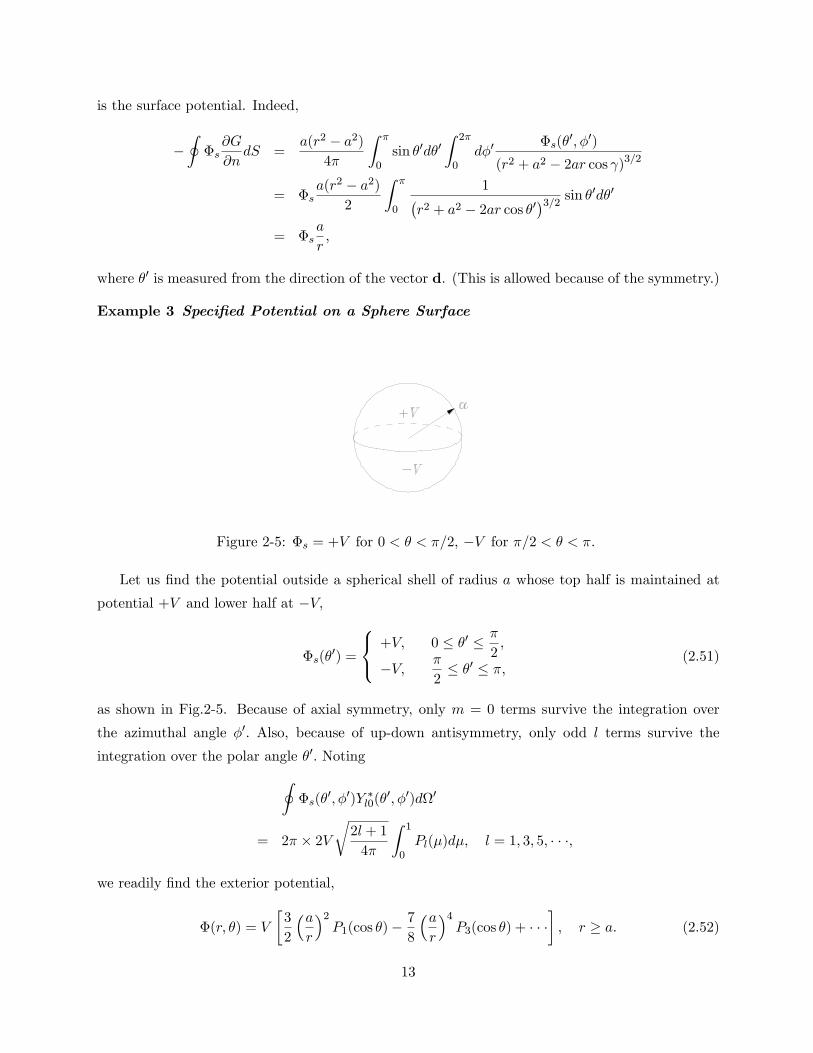
Figure 2-5: Φs = +V for 0 < θ < π/2, −V for π/2 < θ < π.

Let us find the potential outside a spherical shell of radius a whose top half is maintained at

potential +V and lower half at −V,

Φs(θ′) =

+V, 0 ≤ θ′ ≤ π

2,

−V, π

2≤ θ′ ≤ π,

(2.51)

as shown in Fig.2-5. Because of axial symmetry, only m = 0 terms survive the integration over

the azimuthal angle φ′. Also, because of up-down antisymmetry, only odd l terms survive the

integration over the polar angle θ′. Noting∮Φs(θ

′, φ′)Y ∗l0(θ′, φ′)dΩ′

= 2π × 2V

√2l + 1

4π

∫ 1

0Pl(µ)dµ, l = 1, 3, 5, · · ·,

we readily find the exterior potential,

Φ(r, θ) = V

[3

2

(ar

)2P1(cos θ)− 7

8

(ar

)4P3(cos θ) + · · ·

], r ≥ a. (2.52)

13

The interior potential is

Φ(r, θ) = V

[3

2

r

aP1(cos θ)− 7

8

(ra

)3P3(cos θ) + · · ·

], r ≤ a. (2.53)

The surface charge density on the sphere can be found from the normal component of the

electric field,

σ = −ε0∂Φ

∂r

∣∣∣∣r=a+0

=ε0V

a

[3P1(cos θ)− 7

2P3(cos θ) + · · ·

].

The total surface charge on the upper hemisphere

q = 2πa2∫ π/2

0σ(θ) sin θdθ,

simply diverges (albeit only logarithmically) and it is not possible to define the capacitance of the

hemispheres. This is because of the assumption of ideally small gap separating the two hemispheres.

If a small gap δ a is assumed, a finite capacitance containing a factor ln(a/δ) emerges.

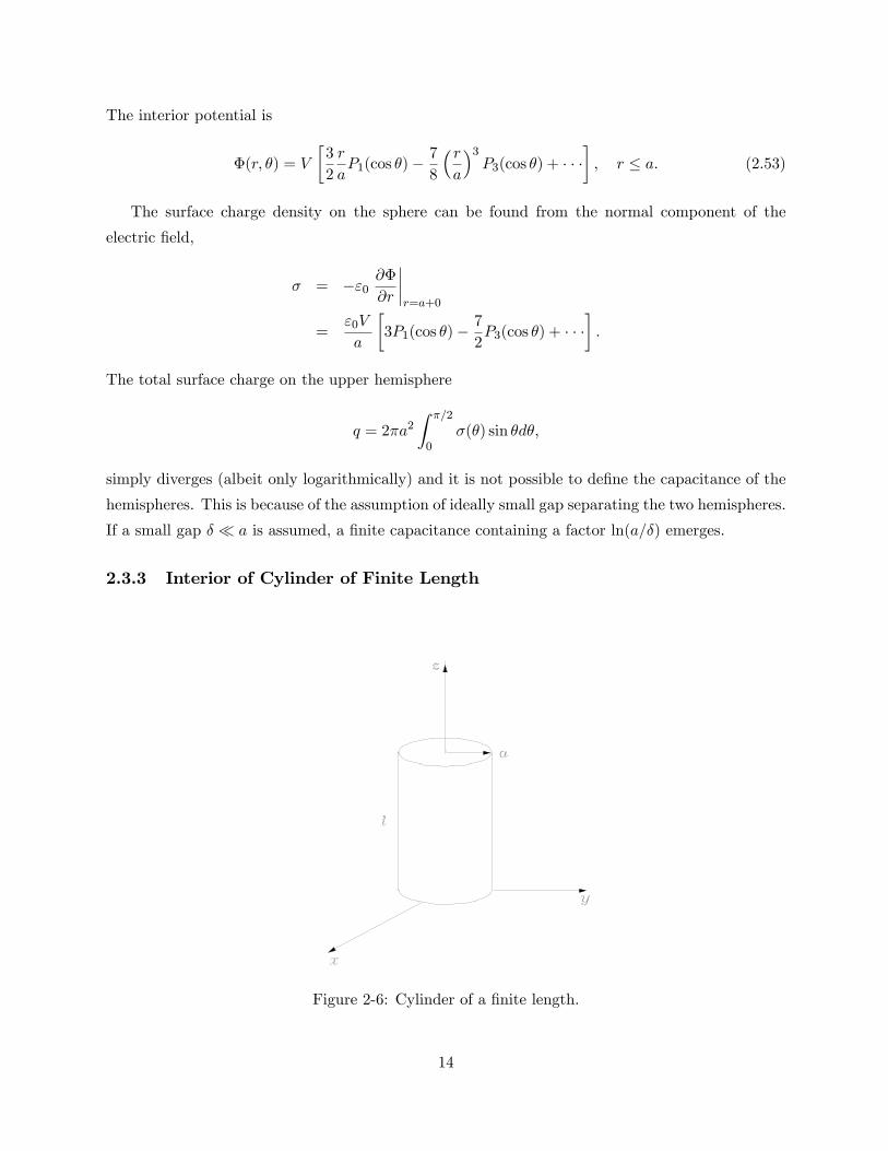
2.3.3 Interior of Cylinder of Finite Length

Figure 2-6: Cylinder of a finite length.

14

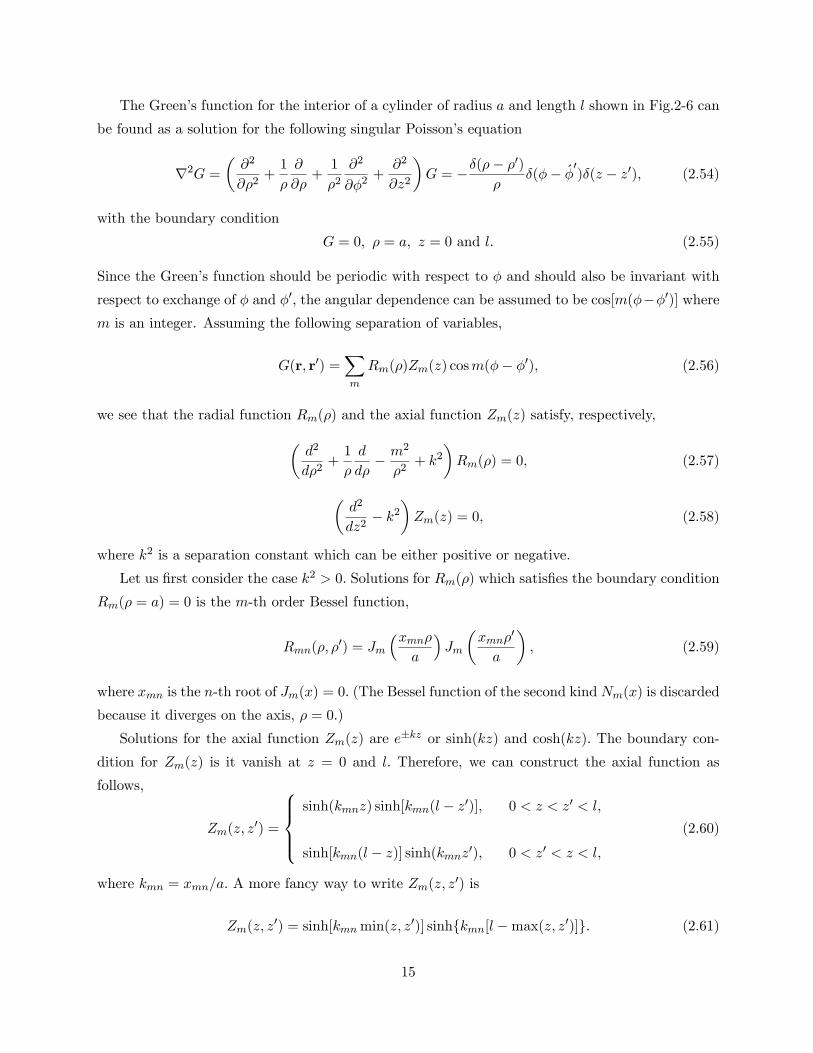
The Green’s function for the interior of a cylinder of radius a and length l shown in Fig.2-6 can

be found as a solution for the following singular Poisson’s equation

∇2G =

(∂2

∂ρ2+

1

ρ

∂

∂ρ+

1

ρ2∂2

∂φ2+

∂2

∂z2

)G = −δ(ρ− ρ

′)

ρδ(φ− φ′)δ(z − z′), (2.54)

with the boundary condition

G = 0, ρ = a, z = 0 and l. (2.55)

Since the Green’s function should be periodic with respect to φ and should also be invariant with

respect to exchange of φ and φ′, the angular dependence can be assumed to be cos[m(φ−φ′)] wherem is an integer. Assuming the following separation of variables,

G(r, r′) =∑m

Rm(ρ)Zm(z) cosm(φ− φ′), (2.56)

we see that the radial function Rm(ρ) and the axial function Zm(z) satisfy, respectively,(d2

dρ2+

1

ρ

d

dρ− m2

ρ2+ k2

)Rm(ρ) = 0, (2.57)

(d2

dz2− k2

)Zm(z) = 0, (2.58)

where k2 is a separation constant which can be either positive or negative.

Let us first consider the case k2 > 0. Solutions for Rm(ρ) which satisfies the boundary condition

Rm(ρ = a) = 0 is the m-th order Bessel function,

Rmn(ρ, ρ′) = Jm

(xmnρa

)Jm

(xmnρ

′

a

), (2.59)

where xmn is the n-th root of Jm(x) = 0. (The Bessel function of the second kind Nm(x) is discarded

because it diverges on the axis, ρ = 0.)

Solutions for the axial function Zm(z) are e±kz or sinh(kz) and cosh(kz). The boundary con-

dition for Zm(z) is it vanish at z = 0 and l. Therefore, we can construct the axial function as

follows,

Zm(z, z′) =

sinh(kmnz) sinh[kmn(l − z′)], 0 < z < z′ < l,

sinh[kmn(l − z)] sinh(kmnz′), 0 < z′ < z < l,

(2.60)

where kmn = xmn/a. A more fancy way to write Zm(z, z′) is

Zm(z, z′) = sinh[kmn min(z, z′)] sinhkmn[l −max(z, z′)]. (2.61)

15

The Green’s function may thus be assumed in the form

G(r, r′) =∑m,n

AmnRmn(ρ, ρ′)Zmn(z, z′) cos[m(φ− φ′)]. (2.62)

The expansion coeffi cient Amn can be determined from the discontinuity in the derivative of the

axial function Zmn(z, z′) at z′,

d

dzZmn

∣∣∣∣z=z′+0

= −kmn cosh[kmn(l − z′)] sinh(kmnz′),

d

dzZmn

∣∣∣∣z=z′−0

= +kmn cosh(kmnz′) sinh[(kmn(l − z′)].

Then, a singularity appears in the second order derivative,

d2

dz2Zmn = −kmn sinh(kmnl)δ(z − z′), (2.63)

which is compatible with the delta function in the RHS of the original singular Poisson’s equation

in Eq. (2.54). Eq. (2.54) now reduces to

∑mn

Amnkmn sinh(kmnl)Jm(kmnρ)Jm(kmnρ′) cosm(φ− φ′) =

δ(ρ− ρ′)ρ

δ(φ− φ′). (2.64)

Multiplying both sides by ρ′Jm(kmnρ′) cosmφ′ and integrating over ρ′ and φ′, we find

A0n =1

πa2kmn

1

J2m+1(kmna) sinh(kmnl), m = 0, (2.65)

Amn =2

πa2kmn

1

J2m+1(kmna) sinh(kmnl), m ≥ 1, (2.66)

where use has been made of the following integral,∫ a

0ρJ2m(kmnρ)dρ =

a2

2J2m+1(kmna). (2.67)

The final form of the desired Green’s function is

G(r, r′) =1

πa

∞∑m=0

∞∑n=1

Jm

(xmnρa

)Jm

(xmnρ

′

a

)Zmn(z, z′)

xmnJ2m+1(xmn) sinh(kmnl)cos[m(φ− φ′)]εm, (2.68)

16

where

εm =

1, m = 0

2, m ≥ 1

If one does not like the appearance of εm, the summation over m can be changed to from −∞ to

∞,

G(r, r′) =1

πa

∞∑m=−∞

∞∑n=1

Jm

(xmnρa

)Jm

(xmnρ

′

a

)Zmn(z, z′)

xmnJ2m+1(xmn) sinh(kmnl)cos[m(φ− φ′)]. (2.69)

If it is assumed that k2 = −κ2 < 0, appropriate general solutions to(d2

dρ2+

1

ρ

d

dρ− m2

ρ2− κ2

)Rm(ρ) = 0, (2.70)

(d2

dz2+ κ2

)Zm(z) = 0, (2.71)

are

Rm(ρ, ρ′

)=

[Km (κma) Im

(κmρ

′)− Im (κma)Km

(κmρ

′)] Im (kmρ) , ρ < ρ′ < a, (2.72)

Rm(ρ, ρ′

)= [Km (κma) Im (κmρ)− Im (κma)Km (κmρ)] Im

(kmρ

′) , ρ′ < ρ < a, (2.73)

with κm = mπ/l and

Zm (z) = sin (κmz) sin(κmz

′) , (2.74)

from which the Green’s function can be constructed. Remaining calculation is left for exercise. The

reader should appreciate how a delta function δ (ρ− ρ′) appears from the term

d2Rmdρ2

. (2.75)

One may wonder about Green’s function for the exterior region of a cylinder of finite length.

This problem appears to be a diffi cult one and analytical expressions are not available to the

author’s knowledge. It may be the case the problem can only be solved numerically.

2.3.4 Long Cylinder (3-Dimensional)

Three dimensional Green’s function for a long cylinder satisfies

∇2G =

(∂2

∂ρ2+

1

ρ

∂

∂ρ+

1

ρ2∂2

∂φ2+

∂2

∂z2

)G = −δ(ρ− ρ

′)

ρδ(φ− φ′)δ(z − z′), (2.76)

17

which is to be solved for the boundary conditions

G(ρ = a) = 0, G(z = ±∞) = 0. (2.77)

Following the same procedure as in the preceding example, the interior solution for interior ρ, ρ′ < a

may be assumed as

G(r, r′) =∑m,n

AmnJm(kmnρ)Jm(kmnρ′) cos[m(φ− φ′)] exp[−kmn|z − z′|], (2.78)

where

kmn =xmna, (2.79)

and xmn is the n-th root of Jm(x) = 0. Since

d2

dz2e−kmn|z−z

′| = k2mne−kmn|z−z′| − 2kmnδ(z − z′), (2.80)

∞∑m=−∞

cos[m(φ− φ′)] = 2πδ(φ− φ′), (2.81)

we readily find the interior Green’s function (ρ, ρ′ < a)

G(r, r′) =1

π

∞∑m=−∞

∞∑n=1

Jm(kmnρ)Jm(kmnρ′)

kmnJ2m+1(kmna)cos[m(φ− φ′)]e−kmn|z−z′|. (2.82)

For exterior of a long cylinder, solutions to the equation(∂2

∂ρ2+

1

ρ

∂

∂ρ+

1

ρ2∂2

∂φ2+

∂2

∂z2

)G = −δ(ρ− ρ

′)

ρδ(φ− φ′)δ(z − z′),

can be found in terms of Fourier transform with respect to the z-coordinate. Let G(r, r′) be

G(r, r′) =∑m

eim(φ−φ′)∫Rm(ρ, ρ′; k)eik(z−z

′)dk. (2.83)

The radial function Rm(ρ, ρ′; k) satisfies(d2

dρ2+

1

ρ

d

dρ− m2

ρ2− k2

)Rm(ρ, ρ′; k) = −δ(ρ− ρ

′)

2πρ. (2.84)

Elementary solutions are the modified Bessel functions Im(kρ) and Km(kρ) and we can construct

18

following solutions which remain bounded in the region a < ρ <∞,

Rm(ρ, ρ′; k) =

A(k)Im(kρ) +B(k)Km(kρ), a < ρ < ρ′ <∞,

C(k)Km(kρ), a < ρ′ < ρ <∞,(2.85)

The boundary conditions are Rm(ρ = a) = 0 and Rm(ρ) be continuous at ρ = ρ′,

A(k)Im(ka) +B(k)Km(ka) = 0, (2.86)

A(k)Im(kρ′) +B(k)Km(kρ′) = C(k)Km(kρ′). (2.87)

Then,

Rm(ρ, ρ′; k) =

A(k)

(Im(kρ)− Im(ka)

Km(ka)Km(kρ)

), a < ρ < ρ′ <∞,

A(k)1

Km(kρ′)

(Im(kρ′)− Im(ka)

Km(ka)Km(kρ′)

)Km(kρ), a < ρ′ < ρ <∞.

(2.88)

The unknown function A(k) can be found from the discontinuity in the derivative at ρ = ρ′,

d2

dρ2Rm(ρ, ρ′; k)

∣∣∣∣ρ=ρ′

= kA(k)K ′m(kρ′)Im(kρ′)−Km(kρ′)I ′m(kρ′)

Km(kρ′)δ(ρ− ρ′) (2.89)

= − A(k)

Km(kρ′)

δ(ρ− ρ′)ρ′

, (2.90)

where again use has been made of the Wronskian of the modified Bessel functions,

I ′m(x)Km(x)− Im(x)K ′m(x) =1

x. (2.91)

We thus find

A(k) =Km(kρ′)

2π, (2.92)

and Rm(ρ, ρ′; k) reduces to

Rm(ρ, ρ′; k) =

1

2πKm(kρ′)

(Im(kρ)− Im(ka)

Km(ka)Km(kρ)

), a < ρ < ρ′ <∞,

1

2π

(Im(kρ′)− Im(ka)

Km(ka)Km(kρ′)

)Km(kρ), a < ρ′ < ρ <∞.

(2.93)

19

The exterior Green’s function of a long cylinder is given by

G(r, r′) =1

2π

∑m

eim(φ−φ′)∫Rm(ρ, ρ′; k)eik(z−z

′)dk. (2.94)

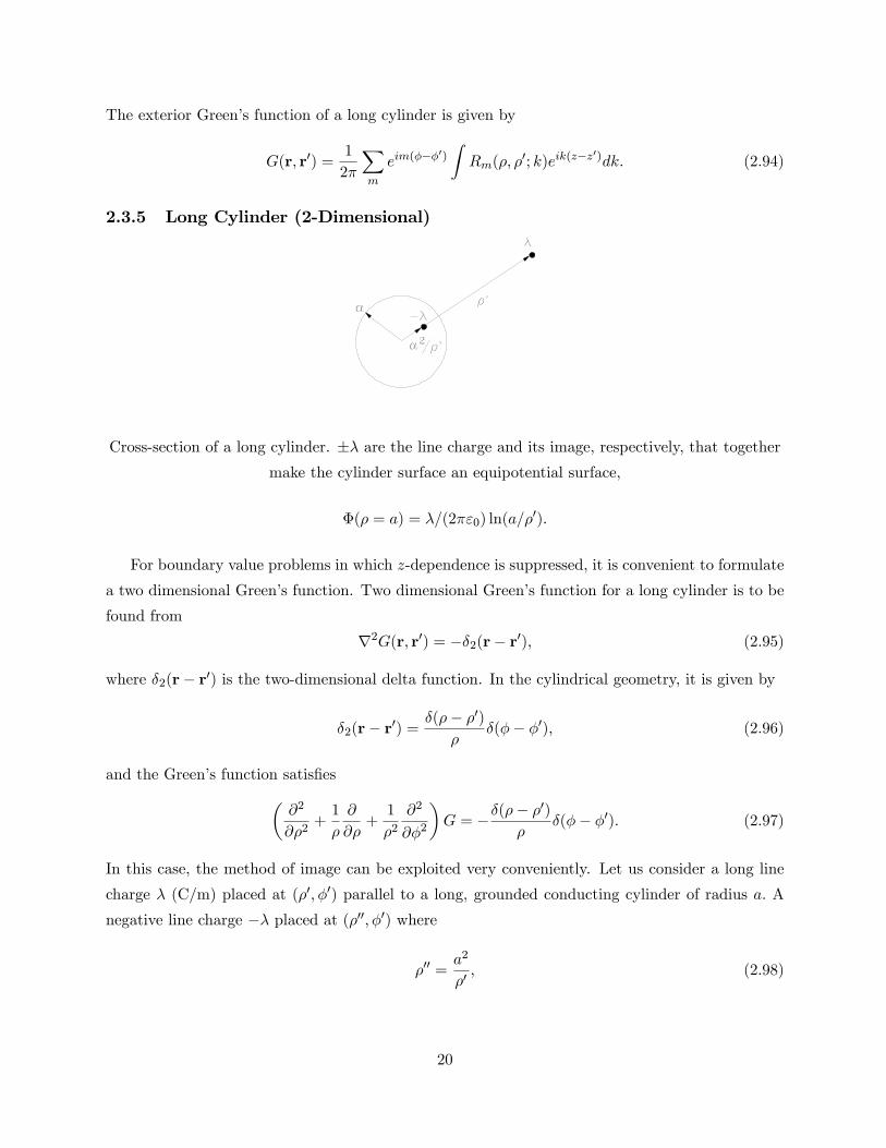
2.3.5 Long Cylinder (2-Dimensional)

Cross-section of a long cylinder. ±λ are the line charge and its image, respectively, that togethermake the cylinder surface an equipotential surface,

Φ(ρ = a) = λ/(2πε0) ln(a/ρ′).

For boundary value problems in which z-dependence is suppressed, it is convenient to formulate

a two dimensional Green’s function. Two dimensional Green’s function for a long cylinder is to be

found from

∇2G(r, r′) = −δ2(r− r′), (2.95)

where δ2(r− r′) is the two-dimensional delta function. In the cylindrical geometry, it is given by

δ2(r− r′) =δ(ρ− ρ′)

ρδ(φ− φ′), (2.96)

and the Green’s function satisfies(∂2

∂ρ2+

1

ρ

∂

∂ρ+

1

ρ2∂2

∂φ2

)G = −δ(ρ− ρ

′)

ρδ(φ− φ′). (2.97)

In this case, the method of image can be exploited very conveniently. Let us consider a long line

charge λ (C/m) placed at (ρ′, φ′) parallel to a long, grounded conducting cylinder of radius a. A

negative line charge −λ placed at (ρ′′, φ′) where

ρ′′ =a2

ρ′, (2.98)

20

makes the cylinder surface an equipotential surface at a potential

Φs =λ

2πε0ln

(a

ρ′

). (2.99)

Since we are seeking a potential that vanishes on the cylinder surface ρ = a, the constant potential

Φs can be subtracted from the potential due to two line charges λ and −λ,

Φ(r, r′) = − λ

2πε0

[ln∣∣r− r′∣∣− ln

∣∣r− r′′∣∣+ ln

(a

ρ′

)], (2.100)

where ∣∣r− r′∣∣ =√ρ2 + ρ′2 − 2ρρ′ cos(φ− φ′), (2.101)

∣∣r− r′′∣∣ =√ρ2 + ρ′′2 − 2ρρ′′ cos(φ− φ′)

=

√ρ2 +

(a2

ρ′

)2− 2

a2ρ

ρ′cos(φ− φ′). (2.102)

The desired Green’s function is

G(r, r′) = − 1

2πln

( √ρ2 + ρ′2 − 2ρρ′ cos(φ− φ′)√

(ρρ′/a)2 + a2 − 2ρρ′ cos(φ− φ′)

). (2.103)

For exterior Dirichlet problems, the normal derivative at the cylinder surface is

∂G

∂n= − ∂G

∂ρ′

∣∣∣∣ρ′=a+0

=1

2π

a− ρ2

aρ2 + a2 − 2aρ cos(φ− φ′) , ρ > a, (2.104)

and for interior,

∂G

∂n=∂G

∂ρ′

∣∣∣∣ρ′=a−0

=1

2π

ρ2

a− a

ρ2 + a2 − 2aρ cos(φ− φ′) , ρ < a. (2.105)

If the potential on a long cylindrical surface is specified as a function of the angle φ, Φs(φ), the

potential off the surface can be calculated from

Φ(ρ, φ) = −a∮

Φs(φ′)∂G

∂ndφ′. (2.106)

21

For the interior (ρ < a) , the potential is given by

Φ(ρ, φ) =1

2π

∫ 2π

0Φs

(φ′) a2 − ρ2a2 + ρ2 − 2aρ cos(φ− φ′)dφ

′

=1

2π

∫ 2π

0Φs

(φ′)(

1 + 2∞∑m=1

(ρa

)mcos[m

(φ− φ′

)]

)dφ′, (2.107)

where use is made of the following expansion,

a2 − ρ2a2 + ρ2 − 2aρ cos(φ− φ′) = 1 + 2

∞∑m=1

(ρa

)mcos[m

(φ− φ′

)].

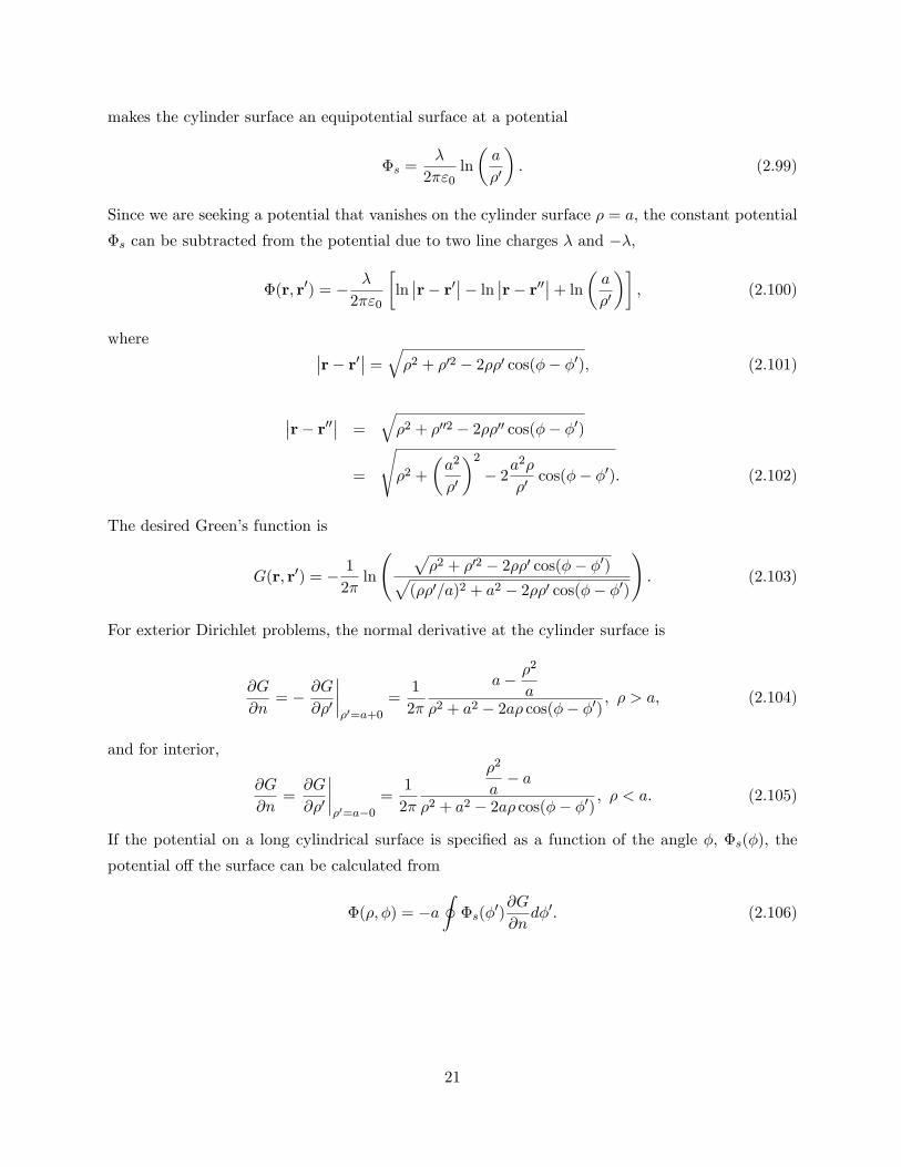
Example 4

Figure 2-7: Φ = V for 0 < φ < π, Φ = −V for −π < φ < 0 on the surface of a long cylinder.(Example of 2-D Green’s function.)

As an example, let us consider a long conducting cylinder consisting of two equal troughs. The

upper half in the region 0 < φ < π is at a potential V and the lower half −π < φ < 0 is at a

potential −V as shown Fig.2-7. The exterior potential ρ > a is given by

Φ(ρ, φ) = Vρ2 − a2

2π

(∫ π

0

1

ρ2 + a2 − 2aρ cos(φ− φ′)dφ′ −∫ 0

−π

1

ρ2 + a2 − 2aρ cos(φ− φ′)dφ′).

(2.108)

22

The first integral can be effected by changing the variable from φ′ to θ through φ′ − π/2 = θ,

∫ π/2

−π/2

1

ρ2 + a2 + 2aρ sin(θ − φ)dθ

=2

ρ2 − a2

tan−1

(ρ2 + a2) tan

(θ − φ

2

)+ 2aρ

ρ2 − a2

π/2

−π/2

=2

ρ2 − a2

[tan−1

((ρ2 + a2)(cotφ− tanφ) + 2aρ

ρ2 − a2

)+ tan−1

((ρ2 + a2)(cotφ+ tanφ) + 2aρ

ρ2 − a2

)]=

2

ρ2 − a2

[tan−1

(2aρ sinφ

ρ2 − a2

)− π

2

], (2.109)

where use has been made of the identities,

tan(π

4± x

2

)= cotx± tanx,

tan−1 x+ tan−1 y = tan−1(x+ y

1− xy

),

tan−1 x =π

2− tan−1

(1

x

).

Similarly, the second integral yields

2

ρ2 − a2

[tan−1

(2aρ sinφ

ρ2 − a2

)+π

2

], (2.110)

and the potential becomes

Φ(ρ, φ) =2V

πtan−1

(2aρ sinφ

ρ2 − a2

), ρ > a. (2.111)

The interior potential is

Φ(ρ, φ) =2V

πtan−1

(2aρ sinφ

a2 − ρ2

), ρ < a. (2.112)

2.3.6 Wedge

A wedge is formed by two large plates intersecting at an angle γ as illustrated in Fig.2-8.

The potential due to a point charge q at (ρ′, φ′, z′) with the boundary conditions Φ = 0 at the

plates φ = 0 and φ = γ, and ρ = ∞, |z| = ∞ essentially gives the Green’s function. We thus seek

23

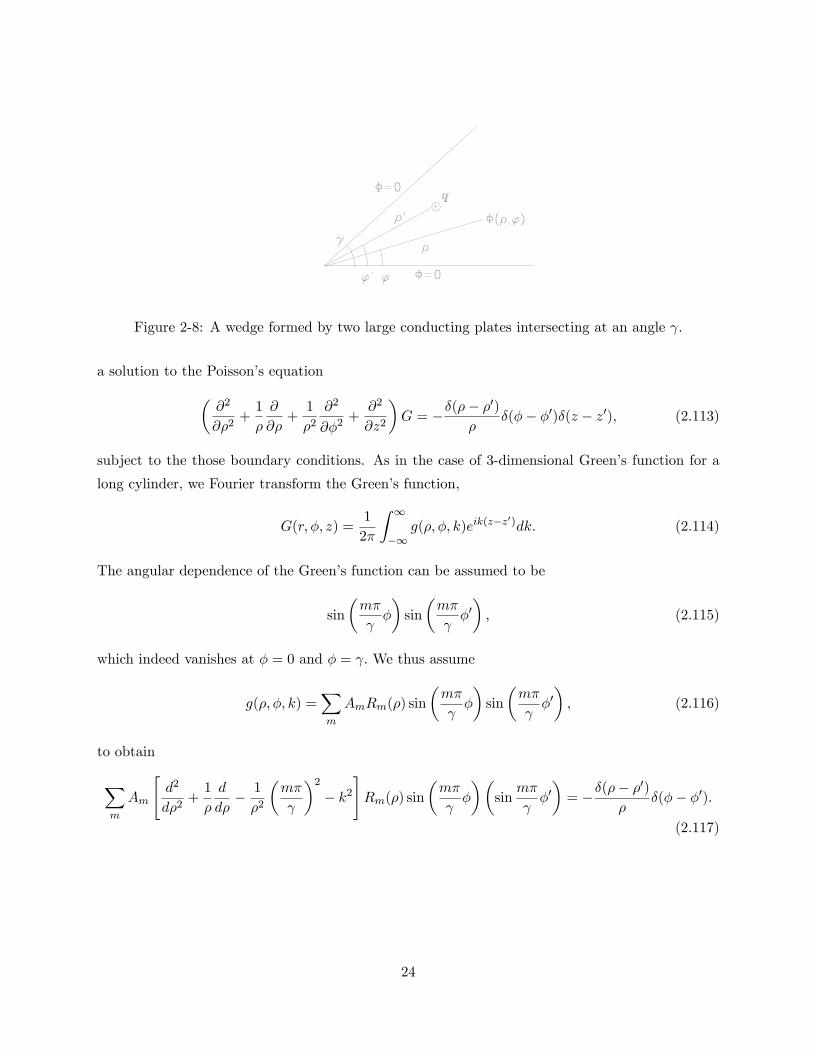
Figure 2-8: A wedge formed by two large conducting plates intersecting at an angle γ.

a solution to the Poisson’s equation(∂2

∂ρ2+

1

ρ

∂

∂ρ+

1

ρ2∂2

∂φ2+

∂2

∂z2

)G = −δ(ρ− ρ

′)

ρδ(φ− φ′)δ(z − z′), (2.113)

subject to the those boundary conditions. As in the case of 3-dimensional Green’s function for a

long cylinder, we Fourier transform the Green’s function,

G(r, φ, z) =1

2π

∫ ∞−∞

g(ρ, φ, k)eik(z−z′)dk. (2.114)

The angular dependence of the Green’s function can be assumed to be

sin

(mπ

γφ

)sin

(mπ

γφ′), (2.115)

which indeed vanishes at φ = 0 and φ = γ. We thus assume

g(ρ, φ, k) =∑m

AmRm(ρ) sin

(mπ

γφ

)sin

(mπ

γφ′), (2.116)

to obtain

∑m

Am

[d2

dρ2+

1

ρ

d

dρ− 1

ρ2

(mπ

γ

)2− k2

]Rm(ρ) sin

(mπ

γφ

)(sin

mπ

γφ′)

= −δ(ρ− ρ′)

ρδ(φ− φ′).

(2.117)

24

The radial function can be composed of the modified Bessel functions,

Rm(ρ) =

Imπ/γ(kρ)Kmπ/γ(kρ′), ρ < ρ′,

Imπ/γ(kρ′)Kmπ/γ(kρ), ρ′ < ρ.

(2.118)

The derivative of the radial function Rm(ρ) has discontinuity at ρ = ρ′, and the second order

derivative yieldsd2Rm(ρ)

dρ2= − 1

ρ′δ(ρ− ρ′), (2.119)

where the Wronskian of the modified Bessel functions,

Iν(x)K ′ν(x)− I ′ν(x)Kν(x) = −1

x,

has been substituted. The expansion coeffi cient Am is thus determined as

Am =1

πγ, (2.120)

and the desired Green’s function is

G(r, r′) =2

πγ

∑m

∫ ∞0

Rm(ρ, ρ′) cos[k(z − z′)]dk sin(νφ) sin(νφ′), (2.121)

where

ν =mπ

γ. (2.122)

We will encounter an application of wedge potential in the section of inversion method later in this

Chapter.

Example 5 Line Charge parallel to a Long Dielectric Cylinder

Consider a long line charge with charge density λ (C m−1) placed parallel to a long dielectric

cylinder of radius a. The distance between the line charge and the cylinder axis is b. The potential

outside the cylinder can be sought by assuming an image line charge λ′ at the position a2/b and

another image −λ′ at the center,

Φρ>a (ρ, φ) = − λ

4πε0ln(ρ2 + b2 − 2ρb cosφ

)− λ′

4πε0ln

(ρ2 +

(a2

b

)2− 2ρ

a2

bcosφ

)+

λ′

4πε0ln ρ2,

where φ is measured relative to the location of line charge λ. The interior potential is free from

25

singularity and may be assumed to be due to an image λ′′ at the location of the line charge λ,

Φρ<a (ρ, φ) = − λ′′

4πε0ln(ρ2 + b2 − 2ρb cosφ

)+

λ′

4πε0ln b2.

Note that the constant potential (the last term)

λ′

4πε0ln b2,

is needed to match same outer potential at r = a,

Φρ>a (r = a) = −λ+ λ′

4πε0ln(a2 + b2 − 2ab cosφ

)+

λ′

4πε0ln b2.

The pertinent boundary conditions are Eφ and Dr be continuous at r = a which yield

λ+ λ′ = λ′′,

and

ε0(λ− λ′

)= ελ′′.

Then

λ′ =ε0 − εε0 + ε

λ, and λ′′ =2ε0ε0 + ε

λ.

The attracting force to act on the unit length of the line charge is given by

F

l=

λ

2πε0

(λ′

b− (a2/b)− λ′′

b

)=

λ2

2πε0

a2

b (b2 − a2)ε0 − εε0 + ε

, (N m−1).

A magnetically dual problem is the case of long current I parallel to a magnetic cylinder with

a permeability µ. The image currents are

I ′ =µ− µ0µ+ µ0

I at ρ =a2

b,

and

I ′′ =2µ

µ+ µ0I at the axis.

2.4 Other Useful Rectilinear Coordinates

The familiar three coordinate systems, cartesian, spherical, and cylindrical, are frequently used in

analyzing potential problems. However, there are some 30 known coordinate systems developed for

specific problems. For simple electrode shapes, potential problems can be rendered one dimensional

26

by a suitable choice of coordinates. However, in some coordinates, solutions to Laplace equations

are not always completely separable. We have encountered one such example in Chapter 1, the

toroidal coordinates, in analyzing the potential due to a ring charge. In this section, some coordinate

systems useful for potential problems will be introduced.

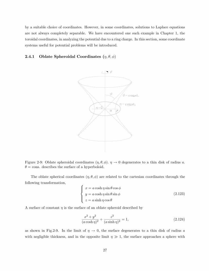
2.4.1 Oblate Spheroidal Coordinates (η, θ, φ)

Figure 2-9: Oblate spheroidal coordinates (η, θ, φ). η → 0 degenerates to a thin disk of radius a.θ = cons. describes the surface of a hyperboloid.

The oblate spherical coordinates (η, θ, φ) are related to the cartesian coordinates through the

following transformation, x = a cosh η sin θ cosφ

y = a cosh η sin θ sinφ

z = a sinh η cos θ

(2.123)

A surface of constant η is the surface of an oblate spheroid described by

x2 + y2

(a cosh η)2+

z2

(a sinh η)2= 1, (2.124)

as shown in Fig.2-9. In the limit of η → 0, the surface degenerates to a thin disk of radius a

with negligible thickness, and in the opposite limit η 1, the surface approaches a sphere with

27

a radius r = a cosh η ' a sinh η. This coordinate system is convenient if electrode shapes are an

oblate sphere or disk. A surface of constant θ is a hyperboloid described by

x2 + y2

(a sin θ)2− z2

(a sin θ)2= 1. (2.125)

The metric coeffi cients are

hη =

√(∂x

∂η

)2+

(∂y

∂η

)2+

(∂z

∂η

)2= a

√cosh2 η − sin2 θ, (2.126)

hθ =

√(∂x

∂θ

)2+

(∂y

∂θ

)2+

(∂z

∂θ

)2= hη, (2.127)

hφ =

√(∂x

∂φ

)2+

(∂y

∂φ

)2+

(∂z

∂φ

)2= a cosh η sin θ. (2.128)

The Laplace equation in the oblate spherical coordinates can thus be written down as

1

hηhθhφ

∂

∂η

(hθhφhη

∂Φ

∂η

)+

∂

∂θ

(hηhφhθ

∂Φ

∂θ

)+

∂

∂φ

(hηhθhφ

∂Φ

∂φ

)= 0, (2.129)

which reduces to

1

cosh2 η − sin2 θ

(∂2

∂η2+ tanh η

∂

∂η+

∂2

∂θ2+ cot θ

∂

∂θ

)Φ +

1

cosh2 η sin2 θ

∂2Φ

∂φ2= 0. (2.130)

Assuming a separated solution Φ(η, θ, φ) = F1(η)F2(θ)eimφ, (m = integer), we obtain(

d2

dη2+ tanh η

d

dη− l(l + 1) +

m2

cosh2 η

)F1(η) = 0, (2.131)

(d2

dθ2+ cot θ

d

dθ+ l(l + 1)− m2

sin2 θ

)F2(θ) = 0, (2.132)

where l(l + 1) is a separation constant. Eq. (2.132) is the standard form of the Legendre equation

and solutions for F2(θ) are

F2(θ) = Pml (cos θ), Qml (cos θ). (2.133)

Eq. (2.131) can be rewritten as(d2

dη2+

sinh η

cosh η

d

dη− l(l + 1) +

m2

1 + sinh2 η

)F1(η) = 0, (2.134)

28

which is also the Legendre equation with a variable i sinh η. Therefore, solutions for F1(η) are

F1(η) = Pml (i sinh η), Qml (i sinh η), (2.135)

and general solution to Laplace equation can be constructed from these elementary solutions.

If a point charge q is placed at(η′, θ′, φ′

), the potential in terms of the oblate spheroidal

coordinates can be found as

Φ(r) =1

4πε0

q

|r− r′|

=q

ε0a

∞∑l=0

l∑m=−l

(l − |m|)!(l + |m|)!

Pml (i sinh η)Qml (i sinh η′)

Pml (i sinh η′)Qml (i sinh η)

Ylm (θ, φ)Y ∗lm

(θ′, φ′

),

η < η′

η > η′

.(2.136)

Derivation of this expression is left for exercise. The Wronskian of the Legendre functions,

Pml (x)d

dxQml (x)−Qml (x)

d

dxPml (x) =

1

x2 − 1

(l + |m|)!(l − |m|)! , (2.137)

should be useful. Furthermore, the Green’s function for an oblate spheroidal surface described by

η = η0 can readily be worked out to be:

for η0 < η < η′,

G(r, r′

)=

1

a

∞∑l=0

l∑m=−l

(l − |m|)!(l + |m|)!P

ml (i sinh η)Qml

(i sinh η′

)Ylm (θ, φ)Y ∗lm

(θ′, φ′

)−1

a

∞∑l=0

l∑m=−l

(l − |m|)!(l + |m|)!

Pml (i sinh η0)

Qml (i sinh η0)Qml (i sinh η)Qml

(i sinh η′

)Ylm (θ, φ)Y ∗lm

(θ′, φ′

),(2.138)

and for η0 < η′ < η,

G(r, r′

)=

1

a

∞∑l=0

l∑m=−l

(l − |m|)!(l + |m|)!P

ml

(i sinh η′

)Qml (i sinh η)Ylm (θ, φ)Y ∗lm

(θ′, φ′

)−1

a

∞∑l=0

l∑m=−l

(l − |m|)!(l + |m|)!

Pml (i sinh η0)

Qml (i sinh η0)Qml (i sinh η)Qml

(i sinh η′

)Ylm (θ, φ)Y ∗lm

(θ′, φ′

).(2.139)

Example 6 Charged Conducting Disk

A thin disk of radius a is described by η = 0 in the oblate spherical coordinates. If a constant

η surface is an equipotential surface, the potential off the surface is a function of η only, that is,

the potential problem becomes one dimensional. This is the most advantageous merit of using a

coordinate system most suitable for particular potential problems. The relevant solution which

29

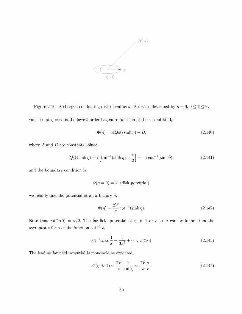
Figure 2-10: A charged conducting disk of radius a. A disk is described by η = 0, 0 ≤ θ ≤ π.

vanishes at η =∞ is the lowest order Legendre function of the second kind,

Φ(η) = AQ0(i sinh η) +B, (2.140)

where A and B are constants. Since

Q0(i sinh η) = i[tan−1(sinh η)− π

2

]= −i cot−1(sinh η), (2.141)

and the boundary condition is

Φ(η = 0) = V (disk potential),

we readily find the potential at an arbitrary η,

Φ(η) =2V

πcot−1(sinh η). (2.142)

Note that cot−1(0) = π/2. The far field potential at η 1 or r a can be found from the

asymptotic form of the function cot−1 x,

cot−1 x ' 1

x− 1

3x3+ · · ·, x 1. (2.143)

The leading far field potential is monopole as expected,

Φ(η 1) ' 2V

π

1

sinh η' 2V

π

a

r. (2.144)

30

Comparing with the standard monopole potential

Φ(r) =1

4πε0

q

r, (2.145)

we readily find the total charge carried by the disk,

q = 8ε0aV,

and the self-capacitance of the disk,

C = 8ε0a, (F). (2.146)

This expression was first found by Cavendish.

The surface charge distribution on the disk is quite nonuniform because like charges repel each

other. Charge is distributed in such a manner that the tangential electric field on the disk surface

vanishes. The surface charge density can be found from the normal component of the electric field,

σ = ε0En = ε0Eη, (2.147)

where

Eη = − 1

hη

∂Φ

∂η

∣∣∣∣η=0

=2V

πa

1

| cos θ| . (2.148)

Note thatd

dxcot−1 x = − 1

1 + x2. (2.149)

The surface charge density diverges at the edge of the disk where θ = π/2. The charge residing on

the disk surface can be found from the following surface integral,

q = ε0

∫ π

0dθ

∫ 2π

0dφσhθhφ

∣∣∣∣η=0

=2ε0aV

π

∫ π

0sin θdθ

∫ 2π

0dφ

= 8ε0aV.

This is consistent with the charge found earlier using the monopole potential.

If one uses a coordinate system other than the oblate spheroidal system, solutions will be much

more involved. Let us employ the cylindrical coordinates (ρ, φ, z). Because of axial symmetry, φ

31

dependence can be suppressed and we seek a solution in the form of Laplace transform,

Φ(ρ, z) =

∫ ∞0Φ(ρ, k)e−k|z|dk. (2.150)

The Laplace equation without φ dependence(∂2

∂ρ2+

1

ρ

∂

∂ρ+

∂2

∂z2

)Φ(ρ, z) = 0, (2.151)

becomes (d2

dρ2+

1

ρ

d

dρ+ k2

)Φ(ρ, k) = 0, (2.152)

which suggests that

Φ(ρ, k) = A(k)J0(kρ). (2.153)

The boundary conditions are:

Φ(ρ ≤ a, z = ±0) = V (constant).

The following integral has a peculiar property,

∫ ∞0

sin ax

xJ0(bx)dx =

π

2, if a > b,

sin−1(a/b), if a < b.

(2.154)

Exploiting this property, we can construct the following solution for the potential,

Φ(ρ, z) =2V

π

∫ ∞0

sin ka

kJ0(kρ)e−k|z|dk. (2.155)

The potential in the disk plane (z = 0) is

Φ(ρ, z = 0) =

V, if ρ < a,

2V

πsin−1(a/ρ), if ρ > a.

(2.156)

Example 7 Dipole Moment of a Conducting Disk in an External Electric Field

If a thin conductor disk is placed perpendicular to an external field, the dipole moment is zero

because of negligible thickness of the disk even though charge separation does take place in such

a manner that disk surfaces are oppositely charged. The external electric field is little disturbed

by the disk in this case. The maximum disturbance occurs when the disk surface is parallel to the

32

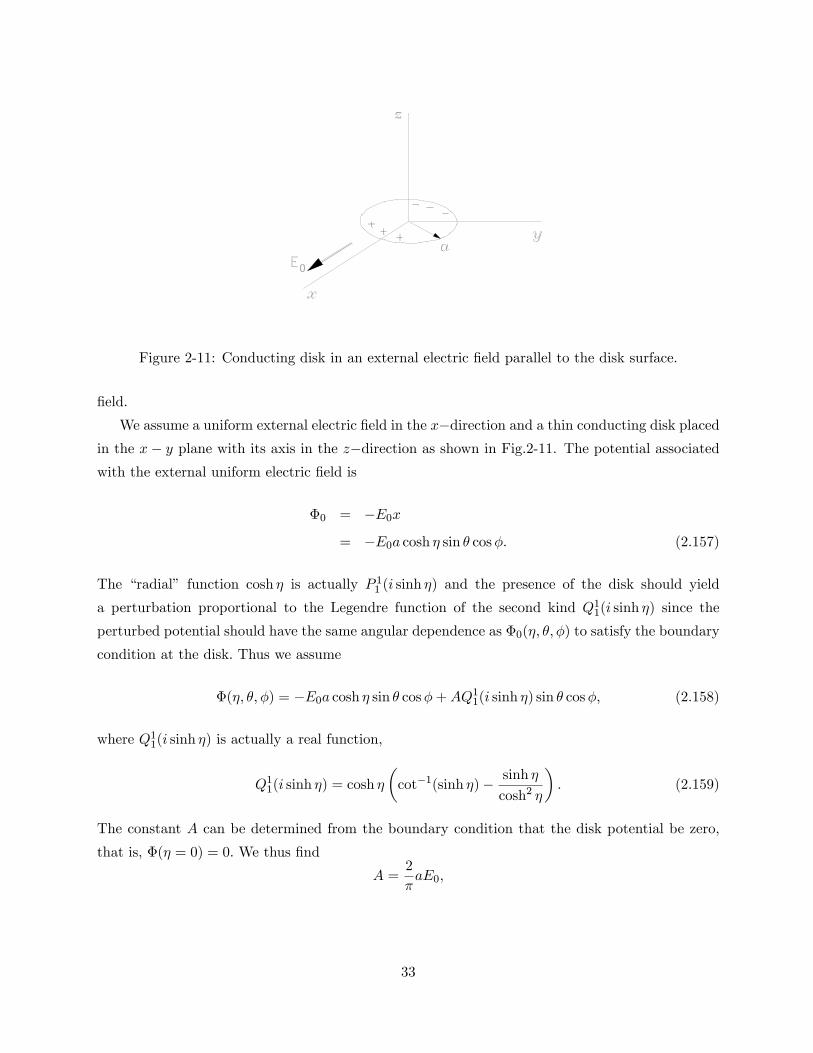
Figure 2-11: Conducting disk in an external electric field parallel to the disk surface.

field.

We assume a uniform external electric field in the x−direction and a thin conducting disk placedin the x− y plane with its axis in the z−direction as shown in Fig.2-11. The potential associatedwith the external uniform electric field is

Φ0 = −E0x

= −E0a cosh η sin θ cosφ. (2.157)

The “radial” function cosh η is actually P 11 (i sinh η) and the presence of the disk should yield

a perturbation proportional to the Legendre function of the second kind Q11(i sinh η) since the

perturbed potential should have the same angular dependence as Φ0(η, θ, φ) to satisfy the boundary

condition at the disk. Thus we assume

Φ(η, θ, φ) = −E0a cosh η sin θ cosφ+AQ11(i sinh η) sin θ cosφ, (2.158)

where Q11(i sinh η) is actually a real function,

Q11(i sinh η) = cosh η

(cot−1(sinh η)− sinh η

cosh2 η

). (2.159)

The constant A can be determined from the boundary condition that the disk potential be zero,

that is, Φ(η = 0) = 0. We thus find

A =2

πaE0,

33

and the potential becomes

Φ(η, θ, φ) = −aE0(

cosh η − 2

πQ11(i sinh η)

)sin θ cosφ. (2.160)

Far away from the disk at r a or η 1, the potential approaches

limη1

Φ(η, θ, φ)→ −aE0 cosh η sin θ cosφ+4E0a

3

3π

sin θ cosφ

r2, (2.161)

where the asymptotic form of Q11(i sinh η),

Q11(i sinh η) ' 2

3

1

sinh2 η=

2

3

(ar

)2, (2.162)

has been substituted. Comparing the dipole term in Eq. (2.161) with the standard dipole potential

Φdipole =1

4πε0

p · rr3

, (2.163)

we can readily identify the dipole moment induced by the disk,

p = 4πε04a3

3πE0‖, (2.164)

where E0‖ is the component of the external electric field tangential to the disk surface. Note that the

dipole moment is proportional to a3. The moment is equally applicable for low frequency oscillating

electric field as long as the wavelength associated with the oscillating filed is much longer than the

disk radius, ka = 2πλ a 1. A resultant scattering cross-section of a conducting disk (sphere too)

placed in a low frequency electromagnetic wave is proportional to a6.

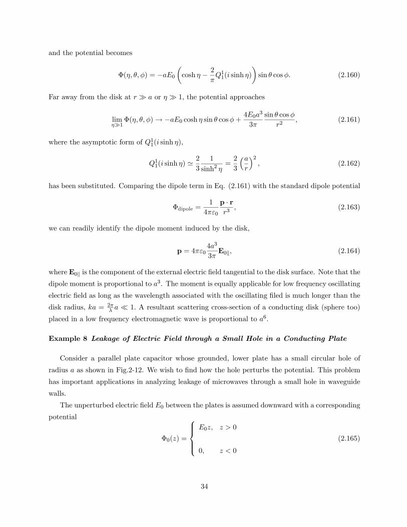
Example 8 Leakage of Electric Field through a Small Hole in a Conducting Plate

Consider a parallel plate capacitor whose grounded, lower plate has a small circular hole of

radius a as shown in Fig.2-12. We wish to find how the hole perturbs the potential. This problem

has important applications in analyzing leakage of microwaves through a small hole in waveguide

walls.

The unperturbed electric field E0 between the plates is assumed downward with a corresponding

potential

Φ0(z) =

E0z, z > 0

0, z < 0

(2.165)

34

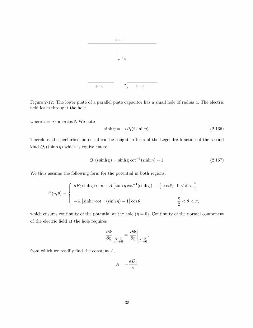
Figure 2-12: The lower plate of a parallel plate capacitor has a small hole of radius a. The electricfield leaks throught the hole.

where z = a sinh η cos θ. We note

sinh η = −iP1(i sinh η). (2.166)

Therefore, the perturbed potential can be sought in term of the Legendre function of the second

kind Q1(i sinh η) which is equivalent to

Q1(i sinh η) = sinh η cot−1(sinh η)− 1. (2.167)

We thus assume the following form for the potential in both regions,

Φ(η, θ) =

aE0 sinh η cos θ +A

[sinh η cot−1(sinh η)− 1

]cos θ, 0 < θ <

π

2

−A[sinh η cot−1(sinh η)− 1

]cos θ,

π

2< θ < π,

which ensures continuity of the potential at the hole (η = 0). Continuity of the normal component

of the electric field at the hole requires

∂Φ

∂η

∣∣∣∣ η=0z=+0

=∂Φ

∂η

∣∣∣∣ η=0z=−0

,

from which we readily find the constant A,

A = −aE0π.

35

In the region below the lower plate (z < 0), the potential is

Φ(η, θ) =aE0π

[sinh η cot−1(sinh η)− 1

]cos θ,

π

2< θ < π. (2.168)

Its asymptotic form is of dipole nature,

Φ(r a)→ −E0a3

3π

1

r2cos θ > 0, (2.169)

(note that cos θ < 0 in the region below the plate) and the effective dipole moment of the hole is

p =4πε0a

3

3πE0, (2.170)

which is downward. The far-field potential in the upper region (z > 0) is

Φ ' Φ0 +E0a

3

3π

1

r2cos θ, (2.171)

in which the dipole term is due to an effective dipole moment upward. The potential at the center

of the hole is

Φ(η = 0, θ = 0 or π) =aE0π. (2.172)

The results of this example, together with those of Example 14 in Chapter 3 (leakage of magnetic

field through a hole in a superconducting plate), will have important implications on diffraction of

electromagnetic waves by an aperture in a conducting plate. Since the effective dipoles are opposite

to each other in the two regions z > 0 and z < 0, it follows in general that

Ez(−z) = −Ez(z),

that is, the electric field normal to the plate is an odd function of z. This means that the surface

charges σ = ε0n ·E (C/m2) induced on both sides of the plate at z = +0 and z = −0 are identical,

where n is the unit normal vector at the plate surface. (Note that n changes its sign from one side

to other.) The component tangential to the plate,

Et = n×E,

is an even function of z,

Et(−z) = Et(z).

Of course, on the surface of the conducting plate, Et vanishes but it does not in the hole. For

36

magnetic fields resulting from a hole in an ideally conducting plate, we will see that the normal

component should vanish at the plate surface

Hz = 0, at z = ±0,

and off the plate, it is even with respect to z,

Hz(−z) = Hz(z),

while the tangential component Ht = n×H is an odd function of z,

Ht(−z) = −Ht(z).

It follows that the surface currents

Js = n×H, (A/m)

on both surfaces of the plate are identical.

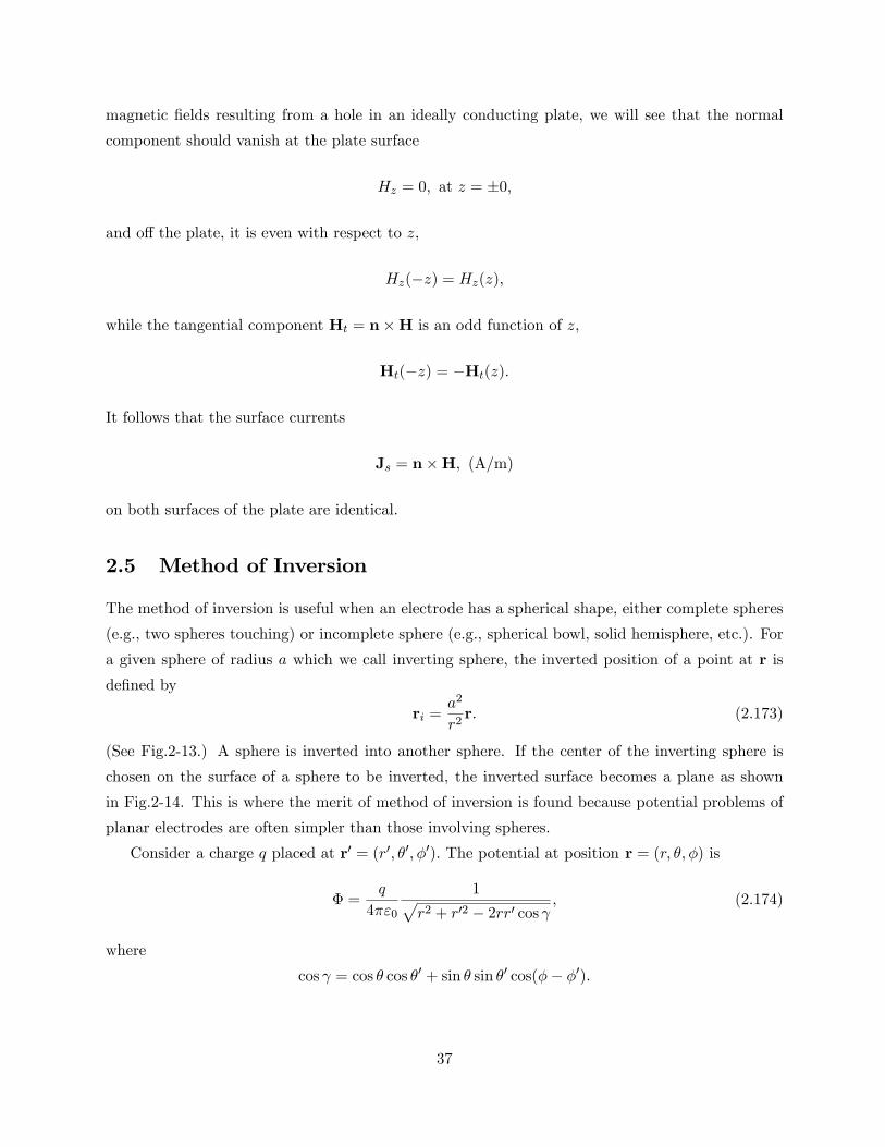
2.5 Method of Inversion

The method of inversion is useful when an electrode has a spherical shape, either complete spheres

(e.g., two spheres touching) or incomplete sphere (e.g., spherical bowl, solid hemisphere, etc.). For

a given sphere of radius a which we call inverting sphere, the inverted position of a point at r is

defined by

ri =a2

r2r. (2.173)

(See Fig.2-13.) A sphere is inverted into another sphere. If the center of the inverting sphere is

chosen on the surface of a sphere to be inverted, the inverted surface becomes a plane as shown

in Fig.2-14. This is where the merit of method of inversion is found because potential problems of

planar electrodes are often simpler than those involving spheres.

Consider a charge q placed at r′ = (r′, θ′, φ′). The potential at position r = (r, θ, φ) is

Φ =q

4πε0

1√r2 + r′2 − 2rr′ cos γ

, (2.174)

where

cos γ = cos θ cos θ′ + sin θ sin θ′ cos(φ− φ′).

37

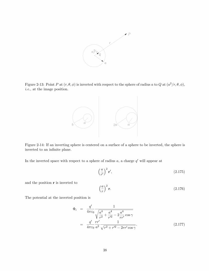
Figure 2-13: Point P at (r, θ, φ) is inverted with respect to the sphere of radius a to Q at (a2/r, θ, φ),i.e., at the image position.

Figure 2-14: If an inverting sphere is centered on a surface of a sphere to be inverted, the sphere isinverted to an infinite plane.

In the inverted space with respect to a sphere of radius a, a charge q′ will appear at( ar′

)2r′, (2.175)

and the position r is inverted to (ar

)2r. (2.176)

The potential at the inverted position is

Φi =q′

4πε0

1√a4

r2+a4

r′2− 2

a4

rr′cos γ

=q′

4πε0

rr′

a21√

r2 + r′2 − 2rr′ cos γ. (2.177)

38

In general, if a function Φ(r, θ, φ) satisfies the Laplace equation, the potential function

a

rΦ

(a2

r, θ, φ

), (2.178)

also satisfies the Laplace equation.

It should be noted that an equipotential spherical surface is in general not inverted to an

equipotential sphere. However, a spherical surface at zero potential is inverted to a zero potential

spherical surface. Since the reference potential can be chosen arbitrarily without affecting the

electric field, one can always choose the potential of an equipotential spherical surface at zero

potential. For example, the potential of a charged conducting sphere of radius a is

Φs =1

4πε0

q

a, (2.179)

relative to zero potential at infinity. However, we can subtract Φs from the potential everywhere

and choose the sphere potential at zero and the potential at infinity as

Φ∞ = − 1

4πε0

q

a.

The electric field remains unchanged through uniform shift of the potential. If an inverting sphere

is chosen in such a way that it has a radius 2a centered at the surface of the conducting sphere of

radius a, the conducting sphere is inverted to an infinite plane touching the both spheres as shown

in Fig. 2-15. Since the sphere potential is chosen at zero, the potential of the plane is also zero.

The potential at infinity is inverted to

− 1

4πε0

q

a× 2a

r= − 1

4πε0

2q

r, (2.180)

where r is the radial distance from the center of the inverting sphere with radius 2a. This is a

potential due to a point charge −2q. Therefore, a charge

−2q = −8πε0Φsa, (2.181)

appears at the center of the inverting sphere.

Example 9 Capacitance of Touching Spheres

Using the method of inversion, we can find the capacitance of two conducting sphere touching

each other as shown in Fig.2-15. The potential of the touching spheres is denoted by Φs. If the

inverting sphere has radius 2a and its center at the touching point, the two spheres become two

39

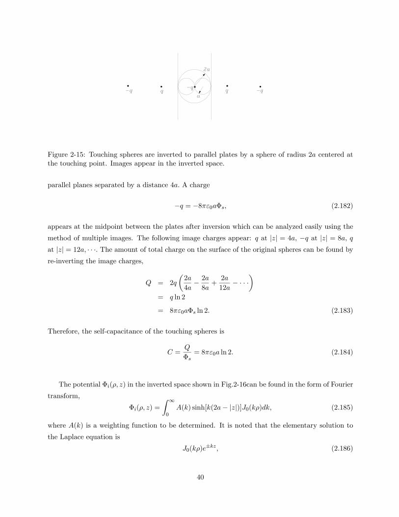
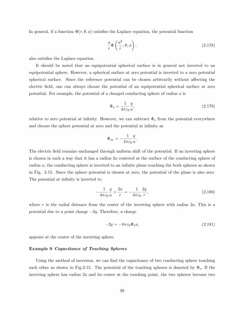
Figure 2-15: Touching spheres are inverted to parallel plates by a sphere of radius 2a centered atthe touching point. Images appear in the inverted space.

parallel planes separated by a distance 4a. A charge

−q = −8πε0aΦs, (2.182)

appears at the midpoint between the plates after inversion which can be analyzed easily using the

method of multiple images. The following image charges appear: q at |z| = 4a, −q at |z| = 8a, q

at |z| = 12a, · · ·. The amount of total charge on the surface of the original spheres can be found byre-inverting the image charges,

Q = 2q

(2a

4a− 2a

8a+

2a

12a− · · ·

)= q ln 2

= 8πε0aΦs ln 2. (2.183)

Therefore, the self-capacitance of the touching spheres is

C =Q

Φs= 8πε0a ln 2. (2.184)

The potential Φi(ρ, z) in the inverted space shown in Fig.2-16can be found in the form of Fourier

transform,

Φi(ρ, z) =

∫ ∞0

A(k) sinh[k(2a− |z|)]J0(kρ)dk, (2.185)

where A(k) is a weighting function to be determined. It is noted that the elementary solution to

the Laplace equation is

J0(kρ)e±kz, (2.186)

40

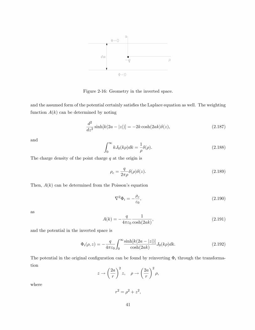
Figure 2-16: Geometry in the inverted space.

and the assumed form of the potential certainly satisfies the Laplace equation as well. The weighting

function A(k) can be determined by noting

d2

dz2sinh[k(2a− |z|)] = −2k cosh(2ak)δ(z), (2.187)

and ∫ ∞0

kJ0(kρ)dk =1

ρδ(ρ). (2.188)

The charge density of the point charge q at the origin is

ρc =q

2πρδ(ρ)δ(z). (2.189)

Then, A(k) can be determined from the Poisson’s equation

∇2Φi = −ρcε0, (2.190)

as

A(k) = − q

4πε0

1

cosh(2ak), (2.191)

and the potential in the inverted space is

Φi(ρ, z) = − q

4πε0

∫ ∞0

sinh[k(2a− |z|)]cosh(2ak)

J0(kρ)dk. (2.192)

The potential in the original configuration can be found by reinverting Φi through the transforma-

tion

z →(

2a

r

)2z, ρ→

(2a

r

)2ρ,

where

r2 = ρ2 + z2,

41

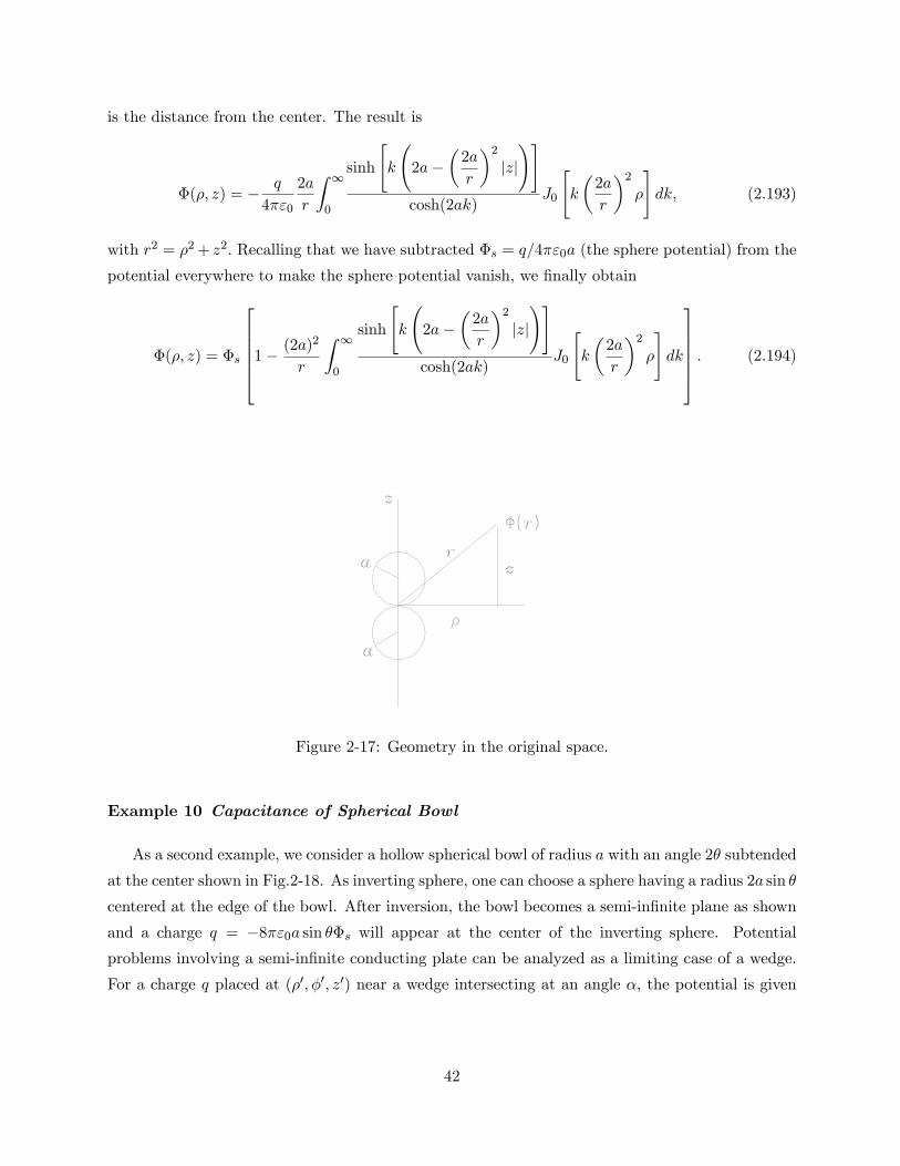
is the distance from the center. The result is

Φ(ρ, z) = − q

4πε0

2a

r

∫ ∞0

sinh

[k

(2a−

(2a

r

)2|z|)]

cosh(2ak)J0

[k

(2a

r

)2ρ

]dk, (2.193)

with r2 = ρ2+ z2. Recalling that we have subtracted Φs = q/4πε0a (the sphere potential) from the

potential everywhere to make the sphere potential vanish, we finally obtain

Φ(ρ, z) = Φs

1− (2a)2

r

∫ ∞0

sinh

[k

(2a−

(2a

r

)2|z|)]

cosh(2ak)J0

[k

(2a

r

)2ρ

]dk

. (2.194)

Figure 2-17: Geometry in the original space.

Example 10 Capacitance of Spherical Bowl

As a second example, we consider a hollow spherical bowl of radius a with an angle 2θ subtended

at the center shown in Fig.2-18. As inverting sphere, one can choose a sphere having a radius 2a sin θ

centered at the edge of the bowl. After inversion, the bowl becomes a semi-infinite plane as shown

and a charge q = −8πε0a sin θΦs will appear at the center of the inverting sphere. Potential

problems involving a semi-infinite conducting plate can be analyzed as a limiting case of a wedge.

For a charge q placed at (ρ′, φ′, z′) near a wedge intersecting at an angle α, the potential is given

42

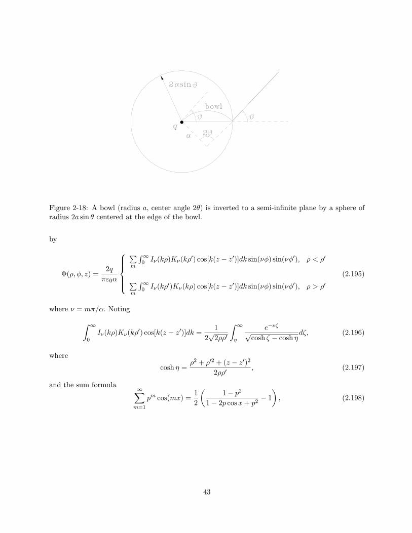
Figure 2-18: A bowl (radius a, center angle 2θ) is inverted to a semi-infinite plane by a sphere ofradius 2a sin θ centered at the edge of the bowl.

by

Φ(ρ, φ, z) =2q

πε0α

∑m

∫∞0 Iν(kρ)Kν(kρ′) cos[k(z − z′)]dk sin(νφ) sin(νφ′), ρ < ρ′

∑m

∫∞0 Iν(kρ′)Kν(kρ) cos[k(z − z′)]dk sin(νφ) sin(νφ′), ρ > ρ′

(2.195)

where ν = mπ/α. Noting∫ ∞0

Iν(kρ)Kν(kρ′) cos[k(z − z′)]dk =1

2√

2ρρ′

∫ ∞η

e−νζ√cosh ζ − cosh η

dζ, (2.196)

where

cosh η =ρ2 + ρ′2 + (z − z′)2

2ρρ′, (2.197)

and the sum formula ∞∑m=1

pm cos(mx) =1

2

(1− p2

1− 2p cosx+ p2− 1

), (2.198)

43

we see that the potential reduces to

Φ(r) =q

4πε0

1

α√

2ρρ′

∫ ∞η

sinh(παζ)

×[

1

cosh(πζ/α)− cos[π(φ− φ′)/α]− 1

cosh(πζ/α)− cos[π(φ+ φ′)/α]

]× 1√

cosh ζ − cosh ηdζ. (2.199)

For a plate α = 2π, and this becomes

Φ(r) =q

4π2ε0

[1

Rcos−1

(−cos[(φ− φ′)/2]

cosh(η/2)

)− 1

R′cos−1

(−cos[(φ+ φ′)/2]

cosh(η/2)

)], (2.200)

where

R =√ρ2 + ρ′2 − 2ρρ′ cos(φ− φ′),

R′ =√ρ2 + ρ′2 − 2ρρ′ cos(φ+ φ′).

The potential in the vicinity of the charge q can be found by letting ρ′ = ρ− r, φ = φ′ = π− θ, η =

r/2a sin θ 1,

Φ(r) =q

4πε0

1

r− q

4πε0

1

4πa sin θ

(1 +

θ

sin θ

), (2.201)

where r is the distance from the charge. The correction due to the presence of the conducting plate

is therefore

∆Φ = − q

4πε0

1

4πa sin θ

(1 +

θ

sin θ

), (2.202)

and in the physical space, the far field potential due to a charged conducting bowl is in the form

Φ(r a) = − q

4πε0

1

2πr

(1 +

θ

sin θ

)=

1

π

a

r(sin θ + θ) Φs. (2.203)

Comparing with the standard monopole potential

Φ =Q

4πε0r,

we finally find the capacitance of the bowl,

C = 4ε0a(θ + sin θ). (2.204)

44

For a sphere, θ = π, we recover C = 4πε0a. For a disk of radius R, θ ' sin θ ' R/a 1, and we

also recover

C = 8ε0R.

The capacitance of a solid (or closed) hemisphere can be found in a similar manner and given

by

C = 8πε0a

(1− 1√

3

). (2.205)

This is left for an exercise.

2.6 Numerical Methods

Analytic solutions in potential problems can only be found for a limited number of applications, and

in practice, it is often necessary to resort to numerical analysis. In this section, we will estimate the

capacitance of a square conductor plate of side a.Mathematically speaking, this problem constitutes

an integral equation for the potential Φ, which is constant at the conductor,

Φ =1

4πε0

∮σ(r′)

|r− r′|dS′ = − 1

4π

∮1

|r− r′|∂Φ

∂n′dS′ = V = constant, (2.206)

where

σ = ε0En = −ε0∂Φ

∂n,

is the unknown surface charge density. The capacitance can be found from

C =1

Φ

∫σdS. (2.207)

As a very rough estimate, we recall that the capacitance of a circular disk of radius a is given

by

C = 8ε0a, (2.208)

and approximate the capacitance of the square plate by

C = 8ε0reff = 8ε0 × 0.564a, (2.209)

where reff is the radius of a circular disk having the same area as the plate,

πr2eff = a2, reff = 0.564a.

The finite element numerical method given below yields C ' 8ε0 × 0.547a.

45

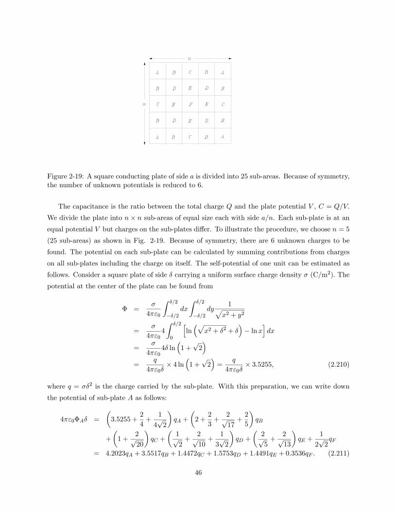
Figure 2-19: A square conducting plate of side a is divided into 25 sub-areas. Because of symmetry,the number of unknown potentials is reduced to 6.

The capacitance is the ratio between the total charge Q and the plate potential V , C = Q/V.

We divide the plate into n× n sub-areas of equal size each with side a/n. Each sub-plate is at anequal potential V but charges on the sub-plates differ. To illustrate the procedure, we choose n = 5

(25 sub-areas) as shown in Fig. 2-19. Because of symmetry, there are 6 unknown charges to be

found. The potential on each sub-plate can be calculated by summing contributions from charges

on all sub-plates including the charge on itself. The self-potential of one unit can be estimated as

follows. Consider a square plate of side δ carrying a uniform surface charge density σ (C/m2). The

potential at the center of the plate can be found from

Φ =σ

4πε0

∫ δ/2

−δ/2dx

∫ δ/2

−δ/2dy

1√x2 + y2

=σ

4πε04

∫ δ/2

0

[ln(√

x2 + δ2 + δ)− lnx

]dx

=σ

4πε04δ ln

(1 +√

2)

=q

4πε0δ× 4 ln

(1 +√

2)

=q

4πε0δ× 3.5255, (2.210)

where q = σδ2 is the charge carried by the sub-plate. With this preparation, we can write down

the potential of sub-plate A as follows:

4πε0ΦAδ =

(3.5255 +

2

4+

1

4√

2

)qA +

(2 +

2

3+

2√17

+2

5

)qB

+

(1 +

2√20

)qC +

(1√2

+2√10

+1

3√

2

)qD +

(2√5

+2√13

)qE +

1

2√

2qF

= 4.2023qA + 3.5517qB + 1.4472qC + 1.5753qD + 1.4491qE + 0.3536qF . (2.211)

46

Other potentials ΦB ∼ ΦF , which are all equal, can be written down in a similar way and we obtain

6 simultaneous equations for qA ∼ qF which can be solved easily. A resultant total charge is

Q = 1.743× 4πε0Φδ,

and the capacitance is

C ' 0.3486× 4πε0a

= 0.547× 8ε0a. (2.212)

Accuracy will improve if a larger number of sub-areas are used.

The method can be applied to estimate the capacitance of a conducting cube as well. With 150

sub-areas (25 sub-areas on each side), the following capacitance emerges,

C ' 0.65× 4πε0a, (2.213)

where a is the side of the cube. An estimate based on a sphere having the same surface area gives

C = 4πε0reff = 0.69× 4πε0a, (2.214)

where

reff =

√6

4πa = 0.69a.

A well known finite element method of solving the Laplace equation is based on the fact that the

potential at the center of a cube may be approximated by the average of 6 surrounding potentials

on each face of the cube,

Φ0 =1

6

6∑i=1

Φi.

This follows from the Taylor expansion of the potential,

Φ(x± δ, y, z) = Φ(x, y, z)± δ ∂Φ

∂x+

1

2

∂2Φ

∂x2± · · ·,

Φ(x, y ± δ, z) = Φ(x, y, z)± δ ∂Φ

∂y+

1

2

∂2Φ

∂y2± · · ·,

Φ(x, y, z ± δ) = Φ(x, y, z)± δ ∂Φ

∂z+

1

2

∂2Φ

∂z2± · · ·,

Adding these 6 equations, we find

Φ(x± δ, y, z) + Φ(x, y ± δ, z) + Φ(x, y, z ± δ) = 6Φ(x, y, z) +∇2Φ +O(δ4). (2.215)

47

Therefore, if Φ satisfies the Laplace equation, ∇2Φ = 0,

Φ center '1

6

6∑i=1

Φi, (2.216)

valid to order δ3.

For 2-dimensional problems in which z-dependence is suppressed, we have

Φcenter '1

4

4∑i=1

Φi. (2.217)

The equation can be applied to each sub-unit having a volume δ3 (3-D) or area δ2 (2-D). Resultant

simultaneous equations can be solved numerically.

Example 11 Potential in a Long Cylinder

Consider a conducting cylinder having a cross-section as shown in Fig. ??. The periodic upper

electrode is at a potential V and the flat lower electrode is grounded. In order to apply the finite

element method, we divide the cross section into sub-sections and allocate 10 nodes points as shown.

Applying Eq. (2.217) to the potentials Φi(i = 1− 10), we obtain

4Φ1 = 100 + Φ2 + 2Φ3,

4Φ2 = Φ1 + 2Φ4,

4Φ3 = 100 + Φ1 + Φ4 + Φ5,

4Φ4 = Φ2 + Φ3 + Φ6,

4Φ5 = 100 + Φ4 + Φ6 + Φ9,

4Φ6 = Φ4 + Φ5 + Φ10,

4Φ7 = 300 + Φ8,

4Φ8 = 200 + Φ7 + Φ9,

4Φ9 = 2Φ5 + Φ8 + Φ10,

4Φ10 = 2Φ6 + Φ9.

Solutions are: Φ1 = 63.7, Φ2 = 31.0, Φ3 = 61.8, Φ4 = 30.2, Φ5 = 53.5, Φ6 = 27.9, Φ7 = 97.1,

Φ8 = 88.2, Φ9 = 55.7, Φ10 = 27.9 all in Volts. A larger number of node points will improve

accuracy.

48

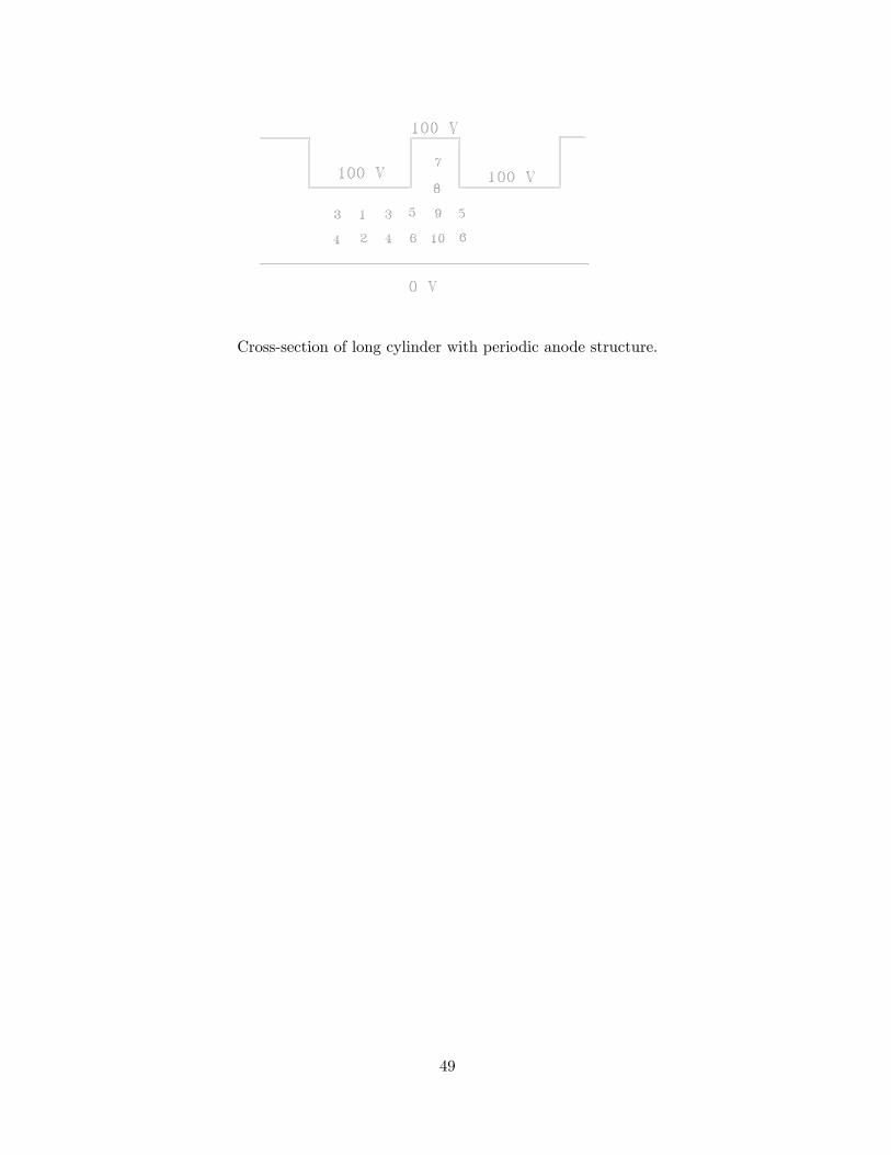
Cross-section of long cylinder with periodic anode structure.

49

Problems

2.1 A ring charge of total charge q and radius b is coaxial with a long grounded conducting

cylinder of radius a (< b). Determine the potential everywhere.

2.2 A ring charge of total charge q and radius b is coaxial with a long uncharged dielectric cylinder

of permittivity ε and radius a. Determine the potential everywhere.

2.3 A charge q is placed at an axial distance b from a conducting disk of radius a. Determine

the potential everywhere. Consider two cases, (a) the disk is grounded, and (b) the disk is

floating.

2.4 Show that a charge q at a distance d from the center of a floating conducting spherical shell

of radius a raises the sphere potential to

Φs =q

4πε0d, if d > a (q outside the sphere),

or

Φs =q

4πε0a, if d < a (q inside).

2.5 A large grounded conducting plate has a hemispherical bob of radius a. A charge q is placed

at an axial distance d from the center of the bob. Find the force on the charge.

2.6 Show that the capacitance per unit length of a parallel wire transmission line with a common

wire radius a and separation distance d is

C

l=

πε0

ln

(d+√d2 − 4a2

2a

) .

2.7 A coaxial cable having inner and outer radii a and b is bent to form a thin toroidal capacitor

with a major radius R ( a, b). Find the capacitance.

2.8 Show that the mutual capacitance between conducting spheres of radii a and b separated by

a large distance d a, b is approximately given by

Cab ' 4πε0ab

d,

and that the capacitance of the sphere of radius a is affected by the sphere of radius b as

Caa ' 4πε0a

(1 +

ab

d2

).

50

2.9 Rigorous analysis of potential problems involving two conducting spheres can be made by

using the bispherical coordinates defined by

x =a sin θ cosφ

cosh η − cos θ,

y =a sin θ sinφ

cosh η − cos θ,

z =a sinh η

cosh η − cos θ.

η = constant surface is a sphere described by

x2 + y2 + (z − acotanhη)2 =

(a

sinh η

)2,

and θ = constant surface is

(ρ− acotanθ)2 + z2 =( a

sin θ

)2,

which is spindle-like shape.

(a) Finding the metric coeffi cients hη, hθ, and hφ, show that the Laplace equation in the

bispherical coordinates is

∂

∂η

(1

cosh η − cos θ

∂Φ

∂η

)+

1

sin θ

∂

∂θ

(sin θ

cosh η − cos θ

∂Φ

∂θ

)+

1

sin2 θ(cosh η − cos θ)

∂2Φ

∂φ2= 0.

(b) Show that the general solution to the Laplace equation is in the form

Φ(η, θ, φ) =√

cosh η − cos θ∑l,m

(Alme(l+ 1

2)η +Blme

−(l+ 12)η)Pml (cosh η)eimφ.

As in the oblate spheroidal coordinates, in this coordinate system too, the Laplace

equation is not separable.

2.10 Using the inversion method, show that the capacitance of a solid or closed conducting hemi-

sphere of radius a is given by

C = 8πε0a

(1− 1√

3

).

2.11 Find a 2D Green’s function for the interior of long cylinder having a semicircular cross-section

of radius a.

51

Hint: Assume

G(r, r′) =

∑mAm(ρ/ρ′)m sin(mφ) sin(mφ′), ρ < ρ′ < a,∑m [Bm(ρ/ρ′)m + Cm(ρ′/ρ)m] sin(mφ) sin(mφ′), ρ′ < ρ < a,

where r = (ρ, φ), r′ = (ρ′, φ′).

2.12 A conducting disk of radius a is placed parallel to an external electric field E0. The dominant

perturbation to the potential is dipole as shown in Example 6. What is the leading higher

order correction?

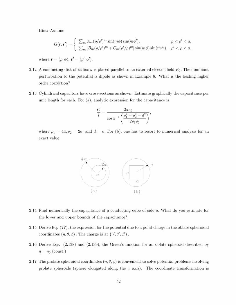
2.13 Cylindrical capacitors have cross-sections as shown. Estimate graphically the capacitance per

unit length for each. For (a), analytic expression for the capacitance is

C

l=

2πε0

cosh−1(ρ21 + ρ22 − d2

2ρ1ρ2

) ,where ρ1 = 4a, ρ2 = 2a, and d = a. For (b), one has to resort to numerical analysis for an

exact value.

2.14 Find numerically the capacitance of a conducting cube of side a. What do you estimate for

the lower and upper bounds of the capacitance?

2.15 Derive Eq. (??), the expression for the potential due to a point charge in the oblate spheroidal

coordinates (η, θ, φ) . The charge is at(η′, θ′, φ′

).

2.16 Derive Eqs. (2.138) and (2.139), the Green’s function for an oblate spheroid described by

η = η0 (const.)

2.17 The prolate spheroidal coordinates (η, θ, φ) is convenient to solve potential problems involving

prolate spheroids (sphere elongated along the z axis). The coordinate transformation is

52

defined by

x = a sinh η sin θ cosφ,

y = a sinh η sin θ sinφ,

z = a cosh η cos θ.

In the limit of η → 0, η = const. surface describes a thin rod having a length 2a, and in the

limit η → ∞, it approaches a sphere with radius a cosh η ' a sinh η. Show that the metric

coeffi cients are:

hη = a

√sinh2 η + cos2 θ = hθ,

hφ = a sinh η cos θ.

Then, show that general solution of Laplace’s equation ∇2Φ = 0 in the prolate spheroidal

coordinates is in the form

Φ (η, θ, φ) =∑l,m

[AlmPml (cosh θ) +BlmQ

ml (cosh η)] [ClmP

ml (cos θ) +DlmQ

ml (cos θ)] eimφ.

In the lowest order l = 0, possible one dimensional solutions are

Φ (η) = Q0 (cosh η) = ln coth(η

2

),

Φ (θ) = Q0 (cos θ) = ln cot

(θ

2

).

53