ANALYSIS OF MIXED ELLIPTIC AND PARABOLIC BOUNDARY LAYERS ...gie/GJT13_IJDE.pdf · ANALYSIS OF MIXED...
26
ANALYSIS OF MIXED ELLIPTIC AND PARABOLIC BOUNDARY LAYERS WITH CORNERS GUNG-MIN GIE 1 , CHANG-YEOL JUNG 2 AND ROGER TEMAM 3 Abstract. We study the asymptotic behavior at small diffusivity of the solutions, u ε , to a convection-diffusion equation in a rectangular domain Ω. The diffusive equation is supplemented with a Dirichlet boundary condition, which is smooth along the edges and continuous at the corners. To resolve the discrepancy, on ∂ Ω, between u ε and the corresponding limit solution, u 0 , we propose asymptotic expan- sions of u ε at any arbitrary, but fixed, order. In order to manage some singular effects near the four corners of Ω, the so-called elliptic and ordinary corner correc- tors are added in the asymptotic expansions as well as the parabolic and classical boundary layer functions. Then, performing the energy estimates on the difference of u ε and the proposed expansions, the validity of our asymptotic expansions is established in suitable Sobolev spaces. 1. Introduction We consider a singularly perturbed convection-diffusion equation in a rectangular domain Ω = (0, 1) × (0, 1): L ε u ε := −εΔu ε − ∂ x u ε = f in Ω, u ε = g on ∂ Ω. (1.1) Here ε is a small but strictly positive diffusivity parameter, and f = f (x, y ) is a given smooth data with ‖D α f ‖ L 2 (Ω) ≤ κ α , independent of ε, for some α’s as needed in the analysis below. The function g = g (x, y ) is assumed to be continuous on ∂ Ω and smooth on each edge of ∂ Ω. Namely, defining the restriction of g to the edges of ∂ Ω as g | x=0 = g 1 (y ), g | x=1 = g 2 (y ), g | y=0 = g 3 (x), g | y=1 = g 4 (x), (1.2) Date : March 30, 2013. 2000 Mathematics Subject Classification. 35B25, 35C20, 76D05, 76D10. Key words and phrases. boundary layers, singular perturbations, convection-dominated equations, corners, corner boundary layers. 1
-
Upload
truongtuong -
Category
Documents
-
view
223 -
download
0
Transcript of ANALYSIS OF MIXED ELLIPTIC AND PARABOLIC BOUNDARY LAYERS ...gie/GJT13_IJDE.pdf · ANALYSIS OF MIXED...
ANALYSIS OF MIXED ELLIPTIC AND PARABOLIC BOUNDARYLAYERS WITH CORNERS
GUNG-MIN GIE1, CHANG-YEOL JUNG2 AND ROGER TEMAM3
Abstract. We study the asymptotic behavior at small diffusivity of the solutions,
uε, to a convection-diffusion equation in a rectangular domain Ω. The diffusive
equation is supplemented with a Dirichlet boundary condition, which is smooth
along the edges and continuous at the corners. To resolve the discrepancy, on ∂Ω,
between uε and the corresponding limit solution, u0, we propose asymptotic expan-
sions of uε at any arbitrary, but fixed, order. In order to manage some singular
effects near the four corners of Ω, the so-called elliptic and ordinary corner correc-
tors are added in the asymptotic expansions as well as the parabolic and classical
boundary layer functions. Then, performing the energy estimates on the difference
of uε and the proposed expansions, the validity of our asymptotic expansions is
established in suitable Sobolev spaces.
1. Introduction
We consider a singularly perturbed convection-diffusion equation in a rectangular
domain Ω = (0, 1)× (0, 1):
Lεuε := −ε∆uε − ∂xu
ε = f in Ω,
uε = g on ∂Ω.(1.1)
Here ε is a small but strictly positive diffusivity parameter, and f = f(x, y) is a given
smooth data with ‖Dαf‖L2(Ω) ≤ κα, independent of ε, for some α’s as needed in the
analysis below. The function g = g(x, y) is assumed to be continuous on ∂Ω and
smooth on each edge of ∂Ω. Namely, defining the restriction of g to the edges of ∂Ω
as
g|x=0 = g1(y), g|x=1 = g2(y), g|y=0 = g3(x), g|y=1 = g4(x),(1.2)
Date: March 30, 2013.2000 Mathematics Subject Classification. 35B25, 35C20, 76D05, 76D10.Key words and phrases. boundary layers, singular perturbations, convection-dominated equations,corners, corner boundary layers.
1
2 G. GIE, C. JUNG AND R. TEMAM
we assume that
g1(0) = g3(0), g1(1) = g4(0), g2(0) = g3(1), g2(1) = g4(1),
gi is smooth for 1 ≤ i ≤ 4.(1.3)
If these compatibility conditions were not satisfied, some additional considerations
would be necessary, which we do not address here.
In what follows, we study the asymptotic behavior of the solutions to (1.1) at small
diffusivity ε.
In a very nice related earlier work, [12], the asymptotic behavior of the solutions
of a convection-diffusion equation similar to (1.1) was discussed. More precisely, in a
rectangular domain Ω = (0, l0)× (0, l1), the authors considered
−ε′∆uε′ − b∂xuε′ + cuε′ = f in Ω,
uε′ = g on ∂Ω,(1.4)
where b > 0, c ≥ 0 are constants, f is a given smooth function in Ω. The function g,
satisfying the analogue version of (1.3) in Ω, is assumed to be continuous and piecewise
smooth on ∂Ω. By constructing, in [12], asymptotic expansions of uε′ with respect to
a small diffusivity ε′, the boundary layers of (1.4) were analyzed in a systematic way.
The validity of their asymptotic expansions were established by using the maximum
principle.
Using a simple change of variables which maps Ω to Ω, and setting uε′ = uεeλx with
a suitable λ, one can transform (1.4) to (1.1) where the two diffusivity parameters ε
and ε′ respectively in (1.1) and (1.4) are compatible, i.e., ε/ε′ is of order one. Hence,
via this transformation, our analysis of (1.1) in this article is applicable to (1.4) as
well. Our motivations for conducting the present study appear below. In particular
we significantly simplify the proofs of [12] and make the study suitable for more
general equations or systems, in particular, those which do not satisfy the maximum
principle.
In the boundary layer analysis associated with the convection-diffusion equation
(1.1) (or (1.4)), one of the most important and difficult point is to resolve any possible
singularity near the four corners of the rectangular domain Ω. Towards this end, we
simplify and improve the method used in [12]. More precisely, concerning the asymp-
totic expansion of uε, we introduce the so-called elliptic boundary layer corrector,
appearing in Section 3.2, near the inflow boundary at x = 1 only, while, in [12], it
was used near both the inflow and outflow boundaries at x = 1 and x = 0. This
simplification in the construction of the asymptotic expansions is mainly based on an
observation that the corner singularities at (0, 0) and (0, 1) (where the flows goes out)
MIXED ELLIPTIC AND PARABOLIC BOUNDARY LAYERS WITH CORNERS 3
can be handled by the ordinary corner corrector, appearing in Section 3.4, (which
is much easier to analyze than the elliptic corrector). Using the energy estimates
rather than the maximum principle as in [12], we prove the validity of our proposed
asymptotic expansions in suitable Sobolev spaces. Here we make use of the Hardy
inequality (see, e.g., [8]) in the estimates. As we said above, our energy estimate
approach can be easily extended to some higher order equations or systems which do
not admit a maximum principle.
This article is organized as follows: In Section 2, we introduce a formal expansion
of uε as the sum of the outer and inner expansions. The outer expansion (outside of
the boundary layers), which is easy to obtain, appears in Section 2. Then, in Section
3, by performing the boundary layer analysis in a systematic way, we construct the
inner expansion (inside the boundary layers). In Section 4, we state and prove the
main convergence result, Theorem 4.1, concerning the difference between uε and the
proposed asymptotic expansion at a given order. In addition, in Appendix A, we
prove Lemma 3.1 that contains some delicate pointwise estimates on the parabolic
boundary layer correctors introduced in Section 3.1. The study of the elliptic corrector
and its approximation also appears in Appendix A.
Throughout this article, we use the notation conventions below.
Notation 1.1.
κ := κ(f, g, Ω, n) is a constant depending on the data, but independent of ε;
here n ≥ 0 is the fixed (but arbitrary) order of the asymptotic expansion, as it appears
in (2.1).
Notation 1.2. An e.s.t. is a function (or a constant) whose norm in all Sobolev
spaces Hs (and thus spaces Cs) is exponentially small with, for each s, a bound of
the form c1 e−c2/εγ , c1, c2, γ > 0, ci, γ depending possibly on s .
Notation 1.3. For a fixed ε > 0, we define the energy norm of H1(Ω),
‖ · ‖ε :=√ε ‖ · ‖H1(Ω) + ‖ · ‖L2(Ω).(1.5)
2. Asymptotic expansions
To study the asymptotic behavior of uε, solution of (1.1), we propose an asymptotic
expansion uε of the following type:
(2.1) uε ∼=n∑
j=0
εj(uj +Θj
).
4 G. GIE, C. JUNG AND R. TEMAM
Here, at each order of εj, j ≥ 0, uj corresponds to the outer expansion (outside of
the boundary layer) of uε. To balance the discrepancy on the boundary ∂Ω of uε
and of the uj, j ≥ 0, we introduce the correctors Θj, j ≥ 0, which will contribute
mainly inside of the boundary layer: Θj will be itself the sum of several boundary
layer functions as we shall see below. The asymptotic expansion (2.1) is made at
order n ≥ 0. As we will see below, the expansion itself depends on n, but n, which is
set at the beginning of the study, can be chosen arbitrary large.
To determine the asymptotic expansion (2.1), we start with the outer expansion
for uε, uε ∼=∑n
j=0 εjuj. Inserting this expansion into (1.1), we formally find the
equations for the uj:
− ∂xu0 = f,(2.2)
− ∂xuj = ∆uj−1, 1 ≤ j ≤ n.(2.3)
We supplement these equations with the inflow boundary conditions (see (1.1)-(1.3)),
u0 = g2(y) at x = 1,(2.4)
uj = 0 at x = 1, 1 ≤ j ≤ n.(2.5)
While the equations (2.2) and (2.3) are “natural”, the choice of the boundary condi-
tions (2.4) and (2.5) is not obvious; it will be eventually justified by the convergence
theorem below. Then, by integrating the equations in x, we find the smooth outer
solutions uj in the form,
u0 =
∫ 1
x
f(x1, y) dx1 + g2(y),(2.6)
uj =
∫ 1
x
∆uj−1(x1, y) dx1, 1 ≤ j ≤ n.(2.7)
Under this construction of the outer expansion, we notice that uε ∼=∑n
j=0 εjuj
satisfies the boundary condition (1.1)2 along the edge x = 1 only, and not on the three
other sides of ∂Ω, y = 0, y = 1 and x = 0 (in general). Hence we expect boundary
layers to occur near those edges, and the so-called correctors (corresponding to the
Θj) will be necessary to account for these discrepancies.
In Section 3, performing the boundary layer analysis, we define, for each 0 ≤ j ≤ n,
the corrector Θj appearing in (3.1) below. Then, in Section 4, using (2.1), (2.6), (2.7)
and (3.1), we prove our main result which is stated as Theorem 4.1.
MIXED ELLIPTIC AND PARABOLIC BOUNDARY LAYERS WITH CORNERS 5
3. Construction of the correctors: boundary layers analysis
We want the boundary value of uε to match that of its approximation. In general,
the boundary values of the diffusive solution uε and the outer expansion∑n
j=0 εjuj
match only at x = 1, but not on the other sides of ∂Ω, y = 0, y = 1 and x = 0.
Hence we expect that some boundary layers will occur near those three edges. To
resolve this inconsistency, we will define a number of boundary layer functions on the
sides and corners of ∂Ω, following an analysis reminiscent of the theory of the Prandtl
boundary layer in [10].
For the moment, comparing uε with a finite sum∑n
j=0 εjuj, we infer from the
definition of the uj in (2.2)-(2.7) that the values of these functions coincide on the
segment x = 1. In general, they will not coincide anywhere else on ∂Ω. First, to
correct the inconsistency on the sides y = 0, 1, we will define the so-called parabolic
correctors ϕj = ϕjl + ϕj
u. Then, to correct the inconsistency at x = 0, we will
introduce the (classical) corrector θj . However, this will not be enough because
additional inconsistencies appear at the corners of Ω, and, as we shall see below,
it will be necessary to introduce additional correctors ξj, ζj and ηj to handle these
inconsistencies.
In summary, in the subsections below, we will define the Θj in the form,
(3.1) Θj = ϕj + ξj + θj + ζj + ηj , 0 ≤ j ≤ n,
where the role and location of each corrector are explained respectively in Table 1
and Figure 1 below. The stretched variables of the corrector functions, which will be
introduced and used in the following subsections, are indicated in Table 2.
ϕj = ϕjl + ϕj
u is the parabolic boundary layer corrector near y = 0 and y = 1,
ξj = ξjl + ξju is the elliptic corrector which resolves the compatibility issues,in the construction of ϕj , at the corners (1, 0) and (1, 1),
θj is the ordinary boundary layer corrector near x = 0,
ζj = ζjl + ζju is the ordinary corner layer corrector which manages the effectof ϕj along x = 0,
ηj = ηjl + ηju is the supplementary corrector that manages the effects of θj
and ζj along the edges y = 0 and y = 1.
Table 1. The different correctors
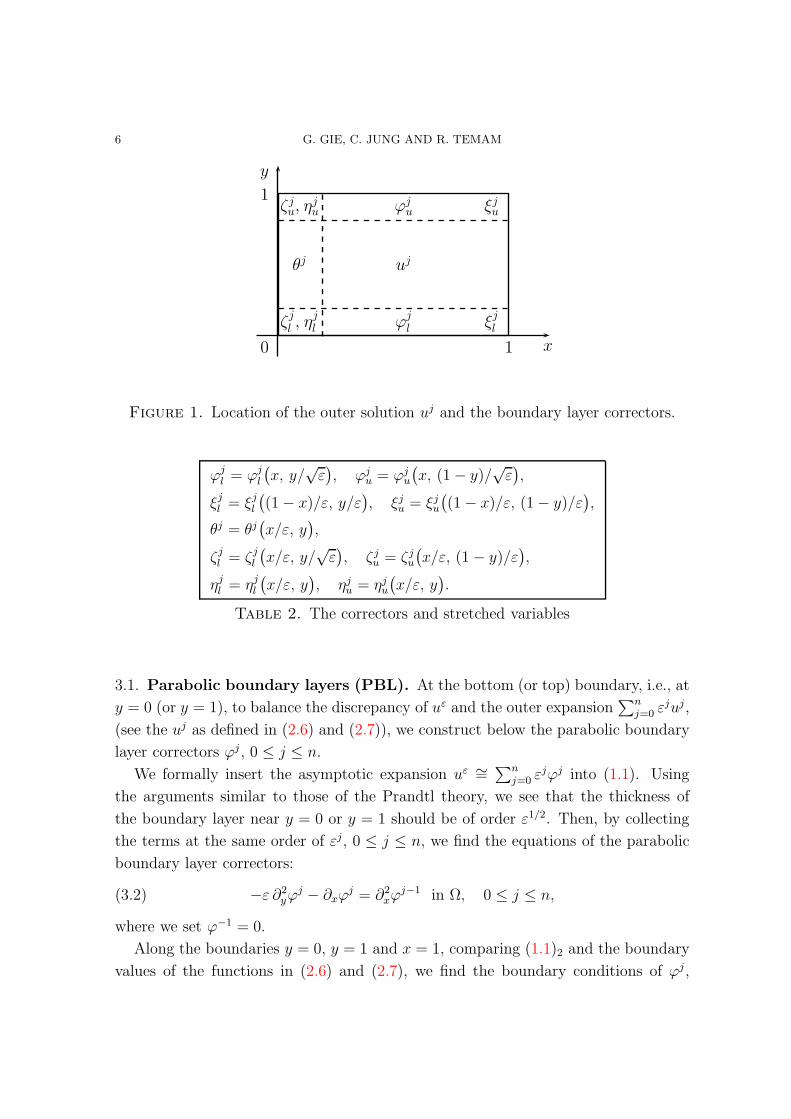
6 G. GIE, C. JUNG AND R. TEMAM
ujθj
ϕju
ϕjl
ξju
ξjl
ηju
ηjlζjl ,
ζju,
0
1
y
1 x
Figure 1. Location of the outer solution uj and the boundary layer correctors.
ϕjl = ϕj
l
(x, y/
√ε), ϕj
u = ϕju
(x, (1− y)/
√ε),
ξjl = ξjl((1− x)/ε, y/ε
), ξju = ξju
((1− x)/ε, (1− y)/ε
),
θj = θj(x/ε, y
),
ζjl = ζjl(x/ε, y/
√ε), ζju = ζju
(x/ε, (1− y)/ε
),
ηjl = ηjl(x/ε, y
), ηju = ηju
(x/ε, y
).
Table 2. The correctors and stretched variables
3.1. Parabolic boundary layers (PBL). At the bottom (or top) boundary, i.e., at
y = 0 (or y = 1), to balance the discrepancy of uε and the outer expansion∑n
j=0 εjuj,
(see the uj as defined in (2.6) and (2.7)), we construct below the parabolic boundary
layer correctors ϕj , 0 ≤ j ≤ n.
We formally insert the asymptotic expansion uε ∼=∑n
j=0 εjϕj into (1.1). Using
the arguments similar to those of the Prandtl theory, we see that the thickness of
the boundary layer near y = 0 or y = 1 should be of order ε1/2. Then, by collecting
the terms at the same order of εj, 0 ≤ j ≤ n, we find the equations of the parabolic
boundary layer correctors:
−ε ∂2yϕ
j − ∂xϕj = ∂2
xϕj−1 in Ω, 0 ≤ j ≤ n,(3.2)
where we set ϕ−1 = 0.
Along the boundaries y = 0, y = 1 and x = 1, comparing (1.1)2 and the boundary
values of the functions in (2.6) and (2.7), we find the boundary conditions of ϕj ,
MIXED ELLIPTIC AND PARABOLIC BOUNDARY LAYERS WITH CORNERS 7
0 ≤ j ≤ n, which read:
(3.3)
ϕj = 0 at x = 1, 0 ≤ j ≤ n,
ϕ0 = g3(x)− u0(x, 0) at y = 0,
ϕj = −uj(x, 0) at y = 0, 1 ≤ j ≤ n,
ϕ0 = g4(x)− u0(x, 1) at y = 1,
ϕj = −uj(x, 1) at y = 1, 1 ≤ j ≤ n.
We will show below how to actually construct ϕj. For the moment, comparing the
functions uε and∑n
j=0 εj(uj − ϕj) for some n ≥ 0, we see that the boundary values
of these functions coincide at x = 1 and y = 0, 1. However this has been achieved at
the price of introducing some new inconsistencies. Indeed we notice, in (3.3), that,
for each j ≥ 0, the boundary conditions at y = 0 and y = 1 are not consistent with
that at x = 1. That is, in general, for any i ≥ 1,
(3.4)
∂ixu
0(1, 0)− ∂ixg3(1) 6= 0, ∂i
xu0(1, 1)− ∂i
xg4(1) 6= 0,
∂ixu
j(1, 0) 6= 0, ∂ixu
j(1, 1) 6= 0, j ≥ 1.
Due to this inconsistency of the boundary data, if we define ϕj , 0 ≤ j ≤ n, as a
solution of (3.2) with (3.3), some derivatives of ϕj , 0 ≤ j ≤ n, get singular at the
two corners (1, k), k = 0, 1. Therefore, to define smooth (smoother) correctors ϕj ,
0 ≤ j ≤ n, we will modify the boundary conditions (3.3) as introduced in (3.13)
below.
3.1.1. On modification of boundary conditions for smooth correctors at y = 0, 1. The
equation (3.2) with initial and boundary conditions (3.3) is a parabolic problem (heat
equation), in which −x is the (positive) time like variable so that the boundary con-
ditions at x = 1 are the analogue of the initial conditions for an evolution problem,
and the possible inconsistencies in (3.4) correspond to the (analogue of ) the compat-
ibility conditions between the initial and boundary values for a parabolic equation;
see [11], [13], [14] and the references therein. Due to the lack of consistency at the
corners (1, 0) and (1, 1), the correctors constructed as in (3.2) and (3.3) might get
singular derivatives at those corners. We will overcome this difficulty by considering
some corner functions at x = 1 and y = 0, 1, similar to what is done in [2], [3] or [4]
for the compatibility issue in parabolic problems; see [5] as well.
8 G. GIE, C. JUNG AND R. TEMAM
Defining δ(x) as a smooth cut-off function, independent of ε, such that
(3.5) δ(x) =
0 for 0 ≤ x ≤ 1/2,
1 for x ≥ 3/4,
we set
(3.6) γjk(x) = γj
k(x) δ(x), k = 0, 1,
where
(3.7)
γ0k(x) =
2n+1∑
i=1
(x− 1)i
i!
[∂ixg3+k(1)− ∂i
xu0(1, k)
],
γjk(x) = −
2n+1−2j∑
i=1
(x− 1)i
i!∂ixu
j(1, k), 1 ≤ j ≤ n.
Note that the γ0k, k = 0, 1, depend on n, but this dependency is not made explicit to
make the notations (slightly) simpler. Note also (comparing to (3.4)) that, at x = 1,
for each k = 0, 1,
(3.8)
γjk(1) = 0, 0 ≤ j ≤ n,
∂ixγ
0k(1) = ∂i
xg3+k(1)− ∂ixu
0(1, k), 1 ≤ i ≤ 2n+ 1,
∂ixγ
jk(1) = −∂i
xuj(1, k), 1 ≤ j ≤ n, 1 ≤ i ≤ 2n+ 1− j.
We introduce the stretched variables,
(3.9) y = y/√ε, y = (1− y)/
√ε.
Then, using (3.2), (3.3), (3.6) and (3.9), we define the parabolic corrector ϕj, 0 ≤j ≤ n, as
(3.10) ϕj = ϕjl + ϕj
u = ϕjl (x, y) + ϕj
u(x, y),
where ϕjl and ϕj
u (lower and upper parts of ϕj respectively) are defined as the solutions
of the 1D heat equations below:
For 0 ≤ j ≤ n,
(3.11)
−∂2yϕ
jl − ∂xϕ
jl = ∂2
xϕj−1l for (y, x) ∈ R
+ × (0, 1),
ϕjl = hj
0(x) at y = 0,
ϕjl → 0 as y → ∞,
ϕjl = 0 at x = 1,
MIXED ELLIPTIC AND PARABOLIC BOUNDARY LAYERS WITH CORNERS 9
(3.12)
−∂2yϕ
ju − ∂xϕ
ju = ∂2
xϕj−1u for (y, x) ∈ R
+ × (0, 1),
ϕju = hj
1(x) at y = 0,
ϕju → 0 as y → ∞,
ϕju = 0 at x = 1.
Here the hjk(x), 0 ≤ j ≤ n, k = 0, 1, are defined by
(3.13)
h00(x) := g3(x)− u0(x, 0)− γ0
0(x),
hj0(x) := −uj(x, 0)− γj
0(x), 1 ≤ j ≤ n,
h01(x) := g4(x)− u0(x, 1)− γ0
1(x),
hj1(x) := −uj(x, 1)− γj
1(x), 1 ≤ j ≤ n.
Note that the smooth boundary conditions hjk(x), 0 ≤ j ≤ n, k = 0, 1, along y or y =
0 are compatible with the other 0 boundary (“initial”) conditions at x = 1 in the
sense that, for each 0 ≤ j ≤ n,
∂ixh
jk(1) = 0, k = 0, 1, 0 ≤ i ≤ 2n+ 1− 2j.
From [1], [9], [6] or [12], we recall the explicit expressions of ϕjl = ϕj
l (x, y), 0 ≤ j ≤n,
(3.14) ϕ0l =
√2
π
∫∞
y/√
2(1−x)
exp(− y21
2
)h00
(x+
y2
2y21
)dy1,
(3.15)
ϕjl =
√2
π
∫∞
y/√
2(1−x)
exp(− y21
2
)hj0
(x+
y2
2y21
)dy1,
+1
2√π
∫ 1−x
0
∫∞
0
1√x1
exp
(− (y − y1)
2
4x1
)− exp
(− (y + y1)
2
4x1
)∂2xϕ
j−1l (x+ x1, y1) dy1dx1.
The expressions of ϕju = ϕj
u(x, y), 0 ≤ j ≤ n, are identical to (3.14) and (3.15) with
h00, h
j0 and y respectively replaced by h0
1, hj1 and y.
3.1.2. Estimates on the parabolic boundary layers. We now state some pointwise es-
timates for the ϕjl and ϕj
u, 0 ≤ j ≤ n, which are proved in Appendix A:
10 G. GIE, C. JUNG AND R. TEMAM
Lemma 3.1. For each 0 ≤ j ≤ n and s ≥ 0, we have the pointwise estimates:
|ys∂ix∂
my ϕj
l | ≤ κεs−m
2 exp(− c
y√ε
), 0 ≤ i+m ≤ 2n+ 2− 2j,(3.16)
|ys∂ix∂
my ϕj
u| ≤ κεs−m
2 exp(− c
1− y√ε
), 0 ≤ i+m ≤ 2n+ 2− 2j,(3.17)
for a generic constant c > 0 independent of x, y and ε.
From Lemma 3.1, it is easy to deduce the following Lp estimates:
Lemma 3.2. For each 0 ≤ j ≤ n and s ≥ 0, we have, for 0 ≤ i+m ≤ 2n+ 2− 2j,
‖ys∂ix∂
my ϕj
l ‖Lp(Ω) + ‖ys∂ix∂
my ϕj
u‖Lp(Ω) ≤ κεs−m
2+ 1
2p .(3.18)
Using (3.10), (3.11) and (3.12), we find the equations for ϕj = ϕjl +ϕj
u, 0 ≤ j ≤ n:
(3.19)
−ε∂2yϕ
j − ∂xϕj = ∂2
xϕj−1 in Ω,
ϕj = hj0(x) + ϕj
u|y=0 at y = 0,
ϕj = hj1(x) + ϕj
l |y=1 at y = 1,
ϕj = 0 at x = 1.
Thanks to Lemma 3.1, we notice that
(3.20) ϕju|y=0 = e.s.t., ϕj
l |y=1 = e.s.t.,
where e.s.t. denotes an exponentially small term with respect to the (small) parameter
ε as defined in Notation 1.2.
3.2. Elliptic boundary layers (EBL). In Section 3.1, to construct the consistent
parabolic boundary layer correctors ϕj , 0 ≤ j ≤ n, we considered the modified
boundary conditions (3.13), including γjk, instead of the natural boundary conditions
(3.3). Here, on the two sides y = 0 and y = 1 of Ω, to cancel γjk which is exactly
the difference of (3.3) and (3.13), we introduce elliptic boundary layer correctors ξj,
0 ≤ j ≤ n, which, like γjk or γj
k, depend on the order n of the asymptotic expansion
in (2.1).
Using (3.6), we define
(3.21) ξj = ξjl + ξju, 0 ≤ j ≤ n,
where ξjl and ξju are the solutions of the elliptic systems below:
MIXED ELLIPTIC AND PARABOLIC BOUNDARY LAYERS WITH CORNERS 11
For 0 ≤ j ≤ n,
(3.22)
−ε ∂2xξ
jl − ε ∂2
yξjl − ∂xξ
jl = 0 in Ω,
ξjl = γj0(x) at y = 0,
ξjl = 0 at x = 0, 1, or y = 1,
(3.23)
−ε ∂2xξ
ju − ε ∂2
yξju − ∂xξ
ju = 0 in Ω,
ξju = γj1(x) at y = 1,
ξju = 0 at x = 0, 1, or y = 0.
The systems (3.22) and (3.23) being elliptic equations, their well-posedness are easy
to verify, and hence we omit the proof here.
The equations satisfied by the elliptic correctors ξj = ξjl + ξju read:
For 0 ≤ j ≤ n,
(3.24)
−ε ∂2xξ
j − ε ∂2yξ
j − ∂xξj = 0 in Ω,
ξj = γjk(x) at y = k , k = 0, 1,
ξj = 0 at x = 0, 1.
In the error analysis below in Section 4, we will see that no extra terms related to
the ξj appear; see (4.6) below. This is because the ξj, as appearing in (3.24), satisfy
the same equation as for uε, supplemented with the (exact) boundary conditions that
we need. From this observation, as it will be justified in Section 4, we notice that our
main result in Theorem 4.1 below does not require any estimate on the ξj.
As an extra information which might be useful elsewhere, but not in this article,
by performing the energy estimate on (3.24), we find that
(3.25) ‖ξj‖ε ≤ κε1
4 , 0 ≤ j ≤ n.
In Appendix A, we introduce an explicit approximate ξ of ξ. Then, thanks to the es-
timates on ξ, one can obtain some pointwise estimates on ξ as well; see the subsection
A.2.
At this stage, the functions uε and∑n
j=0 εj(uj + ϕj + ξj) match along the sides
x = 1 and y = 0, 1 (with singular derivatives of high orders for the ϕj). More precisely,
12 G. GIE, C. JUNG AND R. TEMAM
from (1.1), (2.4), (2.5), (3.19), (3.20) and (3.24), we see that
(3.26) uε −n∑
j=0
εj(uj + ϕj + ξj) =
g1 +
n∑
j=0
εj(uj + ϕj) at x = 0,
0 at x = 1,
n∑
j=0
εjϕju = e.s.t. at y = 0,
n∑
j=0
εjϕjl = e.s.t. at y = 1.
We will now deal with the side x = 0, and construct the ordinary boundary layer
θj and the ordinary corner layer functions (correctors) ζj.
3.3. Ordinary boundary layers (OBL). To handle the discrepancy of uε and∑nj=0 ε
juj at x = 0, which is a part of uε−∑n
j=0 εj(uj +ϕj + ξj) appearing in (3.26),
the so-called ordinary boundary layer corrector θj is introduced in this section. We
insert a formal expansion uε ∼=∑
∞
j=0 εjθj into the diffusive equation (1.1). Then,
using the stretched variable x = x/ε, we find the equations of θj :
−ε∂2xθ
j − ∂xθj = ε−1∂2
yθj−2 in Ω, 0 ≤ j ≤ n,(3.27)
where we set θ−1 = θ−2 = 0.
The main role of the θj is, at each order of εj, to cancel the error uε −∑n
j=0 εjuj
at x = 0. Hence we supplement the equations (3.27) with the boundary conditions,
(3.28)
θ0 = g1(y)− u0(0, y) at x = 0,
θj = −uj(0, y) at x = 0, 1 ≤ j ≤ n,
θj → 0 as x → ∞, 0 ≤ j ≤ n.
The explicit expressions of θj , 0 ≤ j ≤ n, is inductively shown to be of the form,
θj = P k(x/ε, y) exp(−x/ε), j = 2k, 2k + 1,(3.29)
where P k(x/ε, y) is a polynomial in x/ε of degree k whose coefficients, independent
of ε, are linear combinations of the ∂suj−s(0, y)/∂ys, 0 ≤ s ≤ j, and P k(0, y) =
−uj(0, y).
According to (3.29), we deduce the following lemmas:
Lemma 3.3. For each 0 ≤ j ≤ n, we have the pointwise estimates:∣∣xs∂i
x∂my θj∣∣ ≤ κεs−i exp
(−c
x
ε
), s, i,m ≥ 0,(3.30)
MIXED ELLIPTIC AND PARABOLIC BOUNDARY LAYERS WITH CORNERS 13
for a constant c independent of x, y and ε.
Lemma 3.4. For each 0 ≤ j ≤ n, we have∥∥xs∂i
x∂my θj∥∥Lp(Ω)
≤ κεs−i+ 1
p , s, i,m ≥ 0.(3.31)
Thanks to Lemma 3.3, we notice that the effect of θj near the boundary x = 1 is
exponentially small:
(3.32) θj(1, y) = e.s.t., 0 ≤ j ≤ n.
From (3.26), (3.28) and (3.32), we infer that
(3.33)
uε −n∑
j=0
εj(uj + ϕj + ξj + θj) =
n∑
j=0
εjϕj at x = 0,
n∑
j=0
εjθj = e.s.t. at x = 1,
n∑
j=0
εj(ϕju + θj) =
n∑
j=0
εjθj + e.s.t. at y = 0,
n∑
j=0
εj(ϕjl + θj) =
n∑
j=0
εjθj + e.s.t. at y = 1.
3.4. Ordinary corner layers (OCL). To account for the value∑n
j=0 εjϕj at x = 0,
which is exactly the difference of uε and∑n
j=0 εj(uj + ϕj + ξj + θj) at x = 0 (see
(3.33)), we introduce the ordinary corner layer correctors ζj, 0 ≤ j ≤ n, in the form,
(3.34) ζj = ζjl + ζju,
where the ζjl (or ζju) are the correctors near the corner (0, 0) (or (0, 1)) as constructed
below.
To define ζjl (or ζju), we insert a formal expansion uε ∼=∑
∞
j=0 εjζj into (1.1). Then,
using the stretched variables x = x/ε and y = y/√ε near (0, 0), and using x and
y = (1 − y)/√ε near (1, 1), we collect the terms of order εj , 0 ≤ j ≤ n. As a result,
we find the equations for ζjl (or ζju):
(3.35) − ε∂2xζ
jk − ∂xζ
jk = ∂2
yζj−1k in Ω, 0 ≤ j ≤ n, k = u or l.
Here, we set ζ−1k = 0 for k = l, u.
14 G. GIE, C. JUNG AND R. TEMAM
At each order of εj , 0 ≤ j ≤ n, to cancel the error ϕj near the corner (0, 0) or
(0, 1), we supplement the equations (3.35) with the boundary conditions,
(3.36)
ζjk = −ϕj
k(0, y) at x = 0, 0 ≤ j ≤ n, k = l, u,
ζjk → 0 as x → ∞, 0 ≤ j ≤ n, k = l, u.
The explicit solutions ζjl of (3.35) and (3.36), 0 ≤ j ≤ n, are inductively found to
be of the form,
ζjl = P j(x/ε, y/
√ε)exp(−x/ε),(3.37)
where P j(x/ε, y/
√ε)is a polynomial in x/ε of degree j whose coefficients, in-
dependent of ε, are linear combinations of the quantities εs∂2sϕj−sl (0, y/
√ε)/∂y2s,
0 ≤ s ≤ j. In the same manner, the explicit forms of the ζju, 0 ≤ j ≤ n can be found
as well.
Using Lemma 3.1 and (3.37), we obtain the lemmas below:
Lemma 3.5. For each 0 ≤ j ≤ n and k, s ≥ 0, we have the pointwise estimates:
∣∣xkys∂ix∂
my ζjl
∣∣ ≤ κεk−i+ s−m
2 exp(− c(xε+
y√ε
)), 0 ≤ i+m ≤ 2n+ 2− 2j,
(3.38)
∣∣xkys∂ix∂
my ζju
∣∣ ≤ κεk−i+ s−m
2 exp(− c(xε+
1− y√ε
)), 0 ≤ i+m ≤ 2n+ 2− 2j,
(3.39)
for a generic constant c > 0 independent of x, y and ε.
Lemma 3.6. For each 0 ≤ j ≤ n and k, s ≥ 0, we have: for 0 ≤ i+m ≤ 2n+2−2j,∥∥xkys∂i
x∂my ζjl
∥∥Lp(Ω)
+∥∥xkys∂i
x∂my ζju
∥∥Lp(Ω)
≤ κεk−i+ s−m
2+ 3
2p .(3.40)
Thanks to (3.36) and Lemma 3.5, we estimate the values of ζj, 0 ≤ j ≤ n, along
the sides x = 1, y = 0 and y = 1:
(3.41) ζj =
e.s.t. at x = 1,
ζjl (x, 0) + e.s.t. at y = 0,
ζju(x, 1) + e.s.t. at y = 1.
MIXED ELLIPTIC AND PARABOLIC BOUNDARY LAYERS WITH CORNERS 15
Now from (3.33), (3.36) and (3.41), we observe that
(3.42)
uε −n∑
j=0
εj(uj + ϕj + ξj + θj + ζj)
=
0 at x = 0,
n∑
j=0
εj(θj + ζj) = e.s.t. at x = 1,
n∑
j=0
εj(ϕju + θj + ζj) =
n∑
j=0
εj(θj + ζjl ) + e.s.t. at y = 0,
n∑
j=0
εj(ϕjl + θj + ζj) =
n∑
j=0
εj(θj + ζju) + e.s.t. at y = 1.
3.5. Supplementary correctors. Now, our task is to handle, at each order 0 ≤j ≤ n, the effects of θj and ζj along the top and bottom boundaries y = 0, 1. To this
end, using (3.42), we construct the supplementary correctors ηj in the form,
(3.43) ηj = ηjl + ηju, 0 ≤ j ≤ n,
where
ηjl = −(1− y) (θj + ζjl )(x, y = 0), ηju = −y (θj + ζju)(x, y = 1).(3.44)
From Lemmas 3.3 and 3.5, it is easy to verify the lemmas below:
Lemma 3.7. For each 0 ≤ j ≤ n and s ≥ 0, we have the pointwise estimates:
(3.45)∣∣xs∂i
x∂my ηj
∣∣ ≤ κεs−i exp(− c
x
ε
), 0 ≤ i+m ≤ 2n + 2− 2j,
for a constant c independent of x, y and ε.
Lemma 3.8. For each 0 ≤ j ≤ n and s ≥ 0, we have
(3.46)∥∥xs∂i
x∂my ηj
∥∥Lp(Ω)
≤ εs−i+ 1
p , 0 ≤ i+m ≤ 2n+ 2− 2j.
Using (1.3), (3.3), (3.6), (3.11), (3.12), (3.13), (3.28) and (3.36), we find that, near
the corner (0, 0),
(3.47)
(θ0 + ζ0l
)(0, 0) = g1(0)− u0(0, 0)− ϕ0
l (0, 0)
= g1(0)− u0(0, 0)− (g3(0)− u0(0, 0)) = 0.
More generally, one can verify that
(3.48)(θj + ζjl
)(0, 0) = 0,
(θj + ζju
)(0, 1) = 0, 0 ≤ j ≤ n.
16 G. GIE, C. JUNG AND R. TEMAM
Using (3.32), (3.41) and (3.48), we infer from (3.43) and (3.44) that, for 0 ≤ j ≤ n,
(3.49) ηj =
0 at x = 0,
e.s.t. at x = 1,
−(θj + ζjl ) at y = 0,
−(θj + ζju) at y = 1.
Now, we finally obtain from (3.42) and (3.49) that
(3.50)
uε −n∑
j=0
εj(uj + ϕj + ξj + θj + ζj + ηj)
=
0 at x = 0,
n∑
j=0
εj(θj + ζj + ηj) = e.s.t. at x = 1,
n∑
j=0
εj(ϕju + θj + ζj + ηj) =
n∑
j=0
εj(θj + ζjl + ηj) + e.s.t. = e.s.t. at y = 0,
n∑
j=0
εj(ϕjl + θj + ζj + ηj) =
n∑
j=0
εj(θj + ζju + ηj) + e.s.t. = e.s.t. at y = 1.
The e.s.t. on the right hand side of (3.50)2,3,4 are caused respectively by (θj + ζj +ηj)
at x = 1, (ϕju + ζju) at y = 0 and (ϕj
l + ζjl ) at y = 1.
4. Asymptotic error analysis: The main result
We define
(4.1) ρ :=(uε −
n∑
j=0
εj(uj +Θj
))∣∣∣∂Ω
= (the right-hand side of (3.50)),
where Θj = ϕj + ξj + θj + ζj + ηj as defined in (3.1).
We construct an extension ρ of ρ in the form,
(4.2) ρ(x, y) := r+(1−x)(ρ−r)|x=0+x(ρ−r)|x=1+(1−y)(ρ−r)|y=0+y(ρ−r)|y=1,
where
(4.3)
r(x, y) := (1− x)(1− y) ρ|x=y=0 + x(1− y) ρ|x=1, y=0 + (1− x)y ρ|x=0, y=1 + xy ρ|x=y=1.
MIXED ELLIPTIC AND PARABOLIC BOUNDARY LAYERS WITH CORNERS 17
Then one can verify that ρ|∂Ω = ρ and
(4.4) ρ is an e.s.t. in Ω.
We set
(4.5) wεn := uε −n∑
j=0
εj(uj +Θj
)− ρ.
Then, using (1.1), (2.2), (2.3), (3.1), (3.19), (3.24), (3.27), (3.35), (3.44) and (4.1),
the equation of wεn reads:
(4.6)
Lεwεn = εn+1(∆un + ∂2
xϕn + ∂2
yθn + Ξn
1
)
+εn(∂2yθ
n−1 + ε∂2yζ
n + Ξn2
)+ e.s.t. in Ω,
wεn = 0 on ∂Ω,
where
(4.7)
Ξ1 = (1− y) ∂2yθ
n(x, y = 0) + y ∂2yθ
n(x, y = 1),
Ξ2 = (1− y)(∂2yθ
n−1 + ε∂2yζ
nl
)(x, y = 0) + y
(∂2yθ
n−1 + ε∂2yζ
nu
)(x, y = 1).
We multiply (4.6) by exwεn and integrate over Ω. Then, using Lemmas 3.1, 3.3,
3.5 and the Hardy inequality (see, e.g., [8]), we find that
ε|wεn|2H1 +1− ε
2|wεn|2L2
≤ κεn+1
∣∣∣∣∫
Ω
(∆un + ∂2
xϕn + ∂2
yθn + Ξn
1
)wεndxdy
∣∣∣∣
+ κεn∣∣∣∣∫
Ω
x(∂2yθ
n−1 + ε∂2yζ
n + Ξn2
) (wεn
x
)dxdy
∣∣∣∣
≤ κε2n+2 +1
4|wεn|2L2 +
ε
2|wεn|2H1.
(4.8)
Thanks to the elliptic regularity theory and (4.8), we also find that
‖wεn‖H2(Ω) ≤ κ‖∆wεn‖L2(Ω) ≤ κε−1∥∥∂xwεn + lower order terms
∥∥L2(Ω)
≤ κεn−1
2 .
(4.9)
Finally, from (4.4), (4.5), (4.8) and (4.9), we obtain the convergence result on the
difference of uε and the proposed asymptotic expansions, that we summarize in the
theorem below:
Theorem 4.1. For each fixed n ≥ 0, as the diffusivity parameter ε vanishes, the dif-
ference between the solution uε of (1.1) and its asymptotic expansion (2.1) converges
18 G. GIE, C. JUNG AND R. TEMAM
to zero in the following sense:
∥∥∥uε −n∑
j=0
εj(uj +Θj
)∥∥∥ε≤ κεn+1,(4.10)
∥∥∥uε −n∑
j=0
εj(uj +Θj
)∥∥∥H2(Ω)
≤ κεn−1
2 .(4.11)
Remark 4.1. Due to the continuity of g as appearing in (1.3), ξ0 can be omitted in
(3.1) for j = 0 at order ε0. Then one can verify that∥∥uε − (u0 + ϕ0 + θ0 + ζ0 + η0)
∥∥ε≤ κε
3
4 ,(4.12)
which gives a convergence estimate that is a factor of ε1/4 worse than what is stated
in (4.10) for n = 0.
A. APPENDIX
A.1. Proof of Lemma 3.1. To prove (3.16), for y = y/√ε, since ys exp(−cy) ≤
κεs
2 exp(−c0y), ∀y, 0 < c0 < c, it suffices to prove that
|∂ix∂
my ϕj
l | ≤ κ exp
(−c
y√1− x
), 0 ≤ i+m ≤ 2n + 2− 2j, i,m ≥ 0.(A.1)
Note that (3.17) would follow similarly. Since hj(x) = hj0(x) = −uj(x, i) − γj
0(x) for
j ≥ 1 and g3(x)−u0(x, 0)−γ00(x) for j = 0, thanks to (1.3), we note that ∂k
xhj(1) = 0
for 0 ≤ k ≤ 2n+ 1− 2j.
Now, to prove (A.1), we use an induction on j:
(1) We begin with j = 0.
From (3.14), since ∂kxh
0(1) = 0 for 0 ≤ k ≤ 2n + 1, differentiating ϕ0l in x we find
that
|∂ixϕ
0l | =
√2
π
∣∣∣∣∣
∫∞
y/√
2(1−x)
exp
(−y21
2
)∂ixh
0
(x+
y2
2y21
)dy1
∣∣∣∣∣
≤ κ
∫∞
y/√
2(1−x)
exp
(−y21
2
)dy1, 0 ≤ i ≤ 2n+ 2.
(A.2)
Using exp(−y2
1
2
)≤ κ exp (−cy1), ∀y1 ≥ 0, for some c > 0, (A.1) for m = 0 is
proved. Since −ϕ0lyy − ϕ0
lx = 0, for m = 2(k + 1), k ≥ 0, from (A.2) we easily find
that
|∂ix∂
2(k+1)y ϕ0
l | = |∂i+k+1x ϕ0
l | ≤ κ exp
(−c
y√1− x
), 0 ≤ i+ k + 1 ≤ 2n+ 2,(A.3)
MIXED ELLIPTIC AND PARABOLIC BOUNDARY LAYERS WITH CORNERS 19
thus (A.3) holds for 0 ≤ i+m = i+ 2(k + 1) ≤ k + 1+ 2n+ 2, and this implies that
(A.1) holds for m = 2(k + 1), k ≥ 0, j = 0.
Since ∂i+1x h0(1) = 0, 0 ≤ i+ 1 ≤ 2n + 1, we now notice that
|∂ix∂yϕ
0l | =
√2
π
∣∣∣∣∣
∫∞
y/√
2(1−x)
exp
(−y21
2
)∂i+1x h0
(x+
y2
2y21
)y
y21dy1
∣∣∣∣∣
≤ κy
∫∞
y/√
2(1−x)
exp
(−y21
2
)d(−y−1
1 ), 0 ≤ i+ 1 ≤ 2n+ 2.
(A.4)
Integrating by parts in the last integral, we deduce that
|∂ix∂yϕ
0l | ≤ κ
(√1− x exp
(− y2
4(1− x)
)+ y
∫∞
y/√
2(1−x)
exp
(−y21
2
)dy1
)
≤ κ
(exp
(−c
y√1− x
)+ y exp
(−c
y√1− x
))
≤ (since t exp (−ct) ≤ κ exp (−c0t), ∀t ≥ 0, for some 0 < c0 < c)
≤ κ exp
(−c0
y√1− x
), 0 ≤ i+ 1 ≤ 2n + 2.
(A.5)
Hence, for m = 2k + 1, k ≥ 0, using −ϕ0lyy − ϕ0
lx = 0 again, we note from (A.5) that
|∂ix∂
2k+1y ϕ0
l | = |∂i+kx ∂yϕ
0l | ≤ κ exp
(−c
y√1− x
), 0 ≤ i+ k + 1 ≤ 2n+ 2;(A.6)
thus (A.6) holds for 0 ≤ i+m = i+ 2k + 1 ≤ k + 2n + 2, and this proves (A.1) for
m = 2k + 1, k ≥ 0, j = 0. Hence, (A.1) is proved for j = 0.
(2) We now assume that (A.1) holds at any order less than or equal to j − 1, and
we want to prove it at the order j.
At order j ≥ 1, we perform the analysis as follows.
We first note that the homogeneous solution of ϕjl , i.e. the first integral of (3.15) for
ϕjl , can be similarly estimated. We just replace h0
0(x) by hj0(x) in the above analysis.
Since ∂kxh
j(1) = 0 for 0 ≤ k ≤ 2n + 1 − 2j, the first integral is then estimated as
in (A.1) for j = 0. We just replace above 2n + 2 by 2n + 2 − 2j. We now estimate
the particular solution of ϕjl , i.e. the second integral of (3.15) denoted by I. For
simplicity in the analysis below, we write that
J = exp
(−(y − y1)
2
4x1
)− exp
(−(y + y1)
2
4x1
).(A.7)
20 G. GIE, C. JUNG AND R. TEMAM
Using the induction assumption at order j − 1, from (A.1) for j − 1, we note that for
0 ≤ 2 + i ≤ 2n+ 2− 2(j − 1), i.e. 0 ≤ i ≤ 2n+ 2− 2j,
∂2+ix ϕj−1
l (1−, y1) = 0,(A.8)
|∂2+ix ϕj−1
l (x+ x1, y1)| ≤ κ exp
(−c
y1√1− x− x1
)≤ κ exp
(−c
y1√1− x
).(A.9)
Thanks to (A.8), differentiating I, the second integral of (3.15), we find that
∂ixI =
1
2√π
∫ 1−x
0
∫∞
0
J√x1
∂2+ix ϕj−1
l (x+ x1, y1)dy1dx1, 0 ≤ i ≤ 2n+ 2− 2j.(A.10)
Since 0 ≤ x1 ≤ 1− x ≤ 1, |J | ≤ 2 exp(− (y−y1)2
4x1
)≤ 2 exp
(− (y−y1)2
4(1−x)
), from (A.9) we
find that for 0 ≤ i ≤ 2n+ 2− 2j,
|∂ixI| ≤ κ
∫ 1−x
0
1√x1
dx1
∫∞
0
exp
(−(y − y1)
2
4(1− x)
)exp
(−c
y1√1− x
)dy1
≤ (setting β = 2c√1− x)
≤ κ
∫∞
0
exp
(−(y1 − y + β)2
4(1− x)− β
2(1− x)y +
β2
4(1− x)
)dy1
≤ κ exp
(−c
y√1− x
)∫∞
0
exp
(−(y1 − y + β)2
4(1− x)
)dy1
≤ κ exp
(−c
y√1− x
).
(A.11)
This proves (A.1) for m = 0, j ≥ 1.
For m = 2(k+1), k ≥ 0, thanks to the induction assumption on j − 1, from (A.1)
we note that for 0≤ i+s+2+2(k−s)≤2n+2−2(j−1),
|∂i+s+2x ∂
2(k−s)y ϕj−1
l | ≤ κ exp
(−c
y√1− x
),(A.12)
from (A.11) we also note that
|∂i+k+1x I| ≤ κ exp
(−c
y√1− x
), for 0 ≤ i+ k + 1 ≤ 2n+ 2− 2j.(A.13)
Since −Iyy − Ix = ϕj−1lxx , we thus find that
|∂ix∂
2(k+1)y I| ≤ |∂i+k+1
x I|+k∑
s=0
|∂i+s+2x ∂
2(k−s)y ϕj−1
l |
≤ κ exp
(−c
y√1− x
), for 0 ≤ i+ 2(k + 1) ≤ 2n+ 2− 2j.
(A.14)
MIXED ELLIPTIC AND PARABOLIC BOUNDARY LAYERS WITH CORNERS 21
This proves (A.1) for m = 2(k + 1), k ≥ 0, j ≥ 1.
Since ∂y exp(− (y−y1)2
4x1
)= −∂y1 exp
(− (y−y1)2
4x1
), differentiating (A.10) in y we ob-
serve that
|∂ix∂yI| ≤ κ
∣∣∣∣∫ 1−x
0
1√x1
∫∞
0
∂yJ · ∂2+ix ϕj−1
l (x+ x1, y1)dy1dx1
∣∣∣∣
= κ
∣∣∣∣∫ 1−x
0
1√x1
∫∞
0
∂y1 J · ∂2+ix ϕj−1
l (x+ x1, y1)dy1dx1
∣∣∣∣
≤ (integrating by parts in y1)
≤ κ
∣∣∣∣∫ 1−x
0
1√x1
exp
(− y2
4x1
)∂2+ix ϕj−1
l (x+ x1, 0)dx1
∣∣∣∣
+ κ
∣∣∣∣∫ 1−x
0
1√x1
∫∞
0
J · ∂2+ix ∂y1ϕ
j−1l (x+ x1, y1)dy1dx1
∣∣∣∣
(A.15)
where J = exp(− (y−y1)2
4x1
)+ exp
(− (y+y1)2
4x1
)≤ 2 exp
(− (y−y1)2
4(1−x)
). Here, we note that
∂yJ = −∂y1J . Thanks to the induction assumption on j−1, from (A.1) we thus note
that for 0 ≤ 2 + i+ 1 ≤ 2n+ 2− 2(j − 1), i.e. 0 ≤ i ≤ 2n+ 1− 2j,
|∂2+ix ∂y1ϕ
j−1l (x+ x1, y1)| ≤ κ exp
(−c
y1√1− x
),(A.16)
and for 0 ≤ 2 + i ≤ 2n + 2− 2(j − 1), i.e. 0 ≤ i ≤ 2n+ 2− 2j,
|∂2+ix ∂y1ϕ
j−1l (x+ x1, 0)| ≤ κ.(A.17)
As in (A.11) we similarly find that for 0 ≤ i ≤ 2n+ 1− 2j,
|∂ix∂yI| ≤ κ exp
(−c
y√1− x
).(A.18)
Hence, for m = 2k + 1, k ≥ 0, using the induction assumption at order j − 1, from
(A.1) we note that for 0≤ i+s+2+2(k−s)− 1≤2n+2−2(j−1),
|∂i+s+2x ∂
2(k−s)−1y ϕj−1
l | ≤ κ exp
(−c
y√1− x
),(A.19)
from (A.18) we also note that
|∂i+kx ∂yI| ≤ κ exp
(−c
y√1− x
), for 0 ≤ i+ k ≤ 2n+ 1− 2j.(A.20)
22 G. GIE, C. JUNG AND R. TEMAM
Using −Iyy − Ix = ϕj−1lxx again we thus find that
|∂ix∂
2k+1y I| ≤ |∂i+k
x ∂yI|+k−1∑
s=0
|∂i+s+2x ∂
2(k−s)−1y ϕj−1
l |
≤ κ exp
(−c
y√1− x
), for 0 ≤ i+ 2k + 1 ≤ 2n+ 2− 2j.
(A.21)
This proves (A.1) for m = 2k + 1, k ≥ 0, j ≥ 1. Hence, the lemma is proved.
A.2. Study of the elliptic corner correctors ξj = ξjl + ξju. For each 0 ≤ j ≤ n,
using the stretched variables
X = (1− x)/(2ε), Y = y/(2ε),
one can define an approximation ξjl of ξjl as a solution of the system,
−∂2X ξ
jl − ∂2
Y ξjl + 2∂X ξ
jl = 0,
ξjl = 0 at X = 0,
ξjl = γj0(1− 2εX) at Y = 0,
ξjl → 0 at X2 + Y 2 → ∞, Y > 0.
(A.22)
The explicit expression of ξj is given as (see [12])
ξjl =Y
π
∫∞
0
[K1(s1)
s1− K1(s2)
s2
]γj0(1− 2εs) exp (−(s−X)) ds,(A.23)
where K1 is the modified Bessel function of the second kind of the first order, and
s1 =√
(X − s)2 + Y 2, s2 =√
(X + s)2 + Y 2.
Using an appropriate barrier function and the maximum principle (see [12]), one can
verify that∣∣ξjl (X, Y )
∣∣ ≤ κ exp(− c(√
X2 + Y 2 −X))
,(A.24)
for a constant c independent of ε. An approximation ξju of ξju can be constructed in
the same manner.
Using (3.22), (3.23) and (A.24), we notice that ξj − (ξjl + ξju) = e.s.t. at y = 0, 1.
We deduce from (3.6), (3.7) and (A.22)2 that γjk(1) = 0, and hence ξj − (ξjl + ξju) = 0
at x = 1. Moreover, using Lemma A.1 below, we see that ξj − (ξjl + ξju) = 0 at x = 0.
Then, using these observations, thanks to the maximum principle, we find that
(A.25)∣∣ξj − (ξjl + ξju)
∣∣ = e.s.t., 0 ≤ j ≤ n,
MIXED ELLIPTIC AND PARABOLIC BOUNDARY LAYERS WITH CORNERS 23
which implies that the elliptic corrector ξj, 0 ≤ j ≤ n, satisfies the pointwise estimates
similar to (A.24) as for its approximation ξj= ξ
j
l + ξj
u.
Lemma A.1. There exists a positive constant κ, independent of ε, such that∣∣ξj(X, Y )
∣∣ ≤ κminU(X), U(Y ), 0 ≤ j ≤ n,(A.26)
where
U(Z) =
1 if 0 ≤ Z ≤ a,
1− 4(Z − a)2 if a < Z ≤ b,
0 if Z > b,
(A.27)
and a = 38ε, b = a+ 1
2.
To prove Lemma A.1, we will recall below the weak maximum principle (see e.g.
[7]):
We consider an operator L of the form,
Lu =m∑
i,j=1
Di(aijDju) +
m∑
i=1
(Di(biu) + ciDiu) + du,(A.28)
where the coefficients aij, bi, ci, d are assumed to be measurable functions in a domain
Ωm ⊂ Rm, and Di denotes ∂/∂xi, 1 ≤ i ≤ m.
We assume that L is strictly elliptic in Ωm, i.e., there exists λ > 0 such that
m∑
i,j=1
aijξiξj ≥ λ|ξ|2, ∀ξ ∈ Rm,(A.29)
and that L has bounded coefficients, i.e., for some constants Λ and ν ≥ 0, we have
m∑
i,j=1
|aij |2 ≤ Λ2, λ−2m∑
i=1
(|bi|2 + |ci|2) + λ−1|d| ≤ ν2.(A.30)
We also assume that∫
Ωm
(dv −m∑
i=1
biDiv) ≤ 0, ∀v ≥ 0, v ∈ C1c (Ωm).(A.31)
We say that a weakly differentiable function u satisfies Lu = 0, (≥ 0 or ≤ 0), in
the weak sense, if∫
Ωm
( m∑
i,j=1
aijDjuDiv +m∑
i=1
(biuDiv − ciDiuv)− duv)= 0, (≤ 0 or ≥ 0),(A.32)
for all non-negative functions v ∈ C1c (Ωm), provided that aijDju+ biu and ciDiu+du,
1 ≤ i ≤ m, are locally integrable.
24 G. GIE, C. JUNG AND R. TEMAM
Now we state the following maximum principle:
Lemma A.2. Under the conditions (A.29), (A.30) and (A.31), if u ∈ H1(Ωm) sat-
isfies Lu ≥ 0, or Lu ≤ 0, in the weak sense, then we have, respectively,
supΩm
u ≤ sup∂Ωm
u+ or infΩm
u ≥ inf∂Ωm
u−.(A.33)
Thanks to Lemma A.2, we can now prove Lemma A.1:
Proof of Lemma A.1. Given ε0 > 0, thanks to (A.22)4, we may choose a region Ω0 =
(X, Y ) ∈ [0,∞)× [0,∞) | X2 + Y 2 ≤ R2 with R sufficiently large so that |ξj| < ε0
on the circle X2 + Y 2 = R2, X, Y > 0. We then define the barrier function
U = U(X, Y ) = CU(X) + ε0, (X, Y ) ∈ [0,∞)× [0,∞),(A.34)
where U(X) is given in (A.27). Here, C is a positive constant and it will be determined
below. Note that U(X, Y ) ∈ H1(Ω0).
Going back to the elliptic problem (A.22) and writing the elliptic operator L as
Lξj := ξjXX + ξjY Y − 2ξjX ,(A.35)
we find that the operator L satisfies (A.29), (A.30) and (A.31). We also find that for
v ∈ C1c (Ω0), v ≥ 0,
∫
Ω0
(UXvX + UY vY + 2UXv) =
∫ R
0
∫ R
0
C(UXvX + 2UXv)dXdY ≥ 0.(A.36)
Indeed, if 0 ≤ X ≤ a or X > b (a, b as in (A.27)), since UX = 0, we only have
to consider the case a < R ≤ b. For this R, since U ∈ H2(Ω0), we note that∫ R
0(UXvX + 2UXv)dX =
∫ R
0(−UXX + 2UX)vdX =
∫ R
a(−UXX + 2UX)vdX ≥ 0 for all
non-negative v ∈ C1c (Ω0).
Since L(±ξj) = 0, we thus find that L(U ± ξj) ≤ 0 in the weak sense.
Thanks to the cut-off function δ(x), choosing C = maxx∈[ 12,1] |γj(x)|, we find that
U(X, 0) = CU(X) + ε0 ≥ |γj(x)|χ[ 12,1](x)
= |γj(1− 2εX)|χ[0, 1
4ε](X) ≥ |P j(X)| = |ξj(X, 0)|,
(A.37)
U(0, Y ) = C + ε0 ≥ 0 = |ξj(0, Y )|,(A.38)
U(X, Y ) ≥ ε0 > |ξj(X, Y )| on ∂Ω0 with X2 + Y 2 = R2, X, Y > 0.(A.39)
Thus, we note that U ± ξj ≥ 0 on ∂Ω0. Using Lemma A.2 we conclude that, for
(X, Y ) ∈ Ω0,
(U ± ξj)(X, Y ) ≥ infΩ0
(U ± ξj) ≥ inf∂Ω0
(U ± ξj)− = 0.(A.40)
MIXED ELLIPTIC AND PARABOLIC BOUNDARY LAYERS WITH CORNERS 25
Hence, we have
|ξj(X, Y )| ≤ U(X, Y ) = CU(X) + ε0.(A.41)
Letting R → ∞, we deduce that |ξj(X, Y )| ≤ CU(X). Similarly, we can conclude
that |ξj(X, Y )| ≤ CU(Y ). This proves the lemma.
Acknowledgments
This work was supported in part by the Research Fund of Indiana University, by
NSF Grants DMS 0906440, DMS 1206438 and DMS 1212141, and by Basic Science
Research Program through the National Research Foundation of Korea (NRF) funded
by the Ministry of Education, Science and Technology (2012001167).
References
[1] John Rozier Cannon. The one-dimensional heat equation, volume 23 of Encyclopedia of Math-
ematics and its Applications. Addison-Wesley Publishing Company Advanced Book Program,
Reading, MA, 1984. With a foreword by Felix E. Browder. 9
[2] Qingshan Chen, Zhen Qin, and Roger Temam. Numerical resolution near t = 0 of nonlinear
evolution equations in the presence of corner singularities in space dimension 1. Commun.
Comput. Phys., 9(3):568–586, 2011. 7
[3] Natasha Flyer and Bengt Fornberg. Accurate numerical resolution of transients in initial-
boundary value problems for the heat equation. J. Comput. Phys., 184(2):526–539, 2003. 7
[4] Natasha Flyer and Bengt Fornberg. On the nature of initial-boundary value solutions for dis-
persive equations. SIAM J. Appl. Math., 64(2):546–564 (electronic), 2003/04. 7
[5] Gung-Min Gie. Asymptotic expansion of the Stokes solutions at small viscosity: the case of
non-compatible initial data. Submitted. 7
[6] Gung-Min Gie, Makram Hamouda, and Roger Temam. Boundary layers in smooth curvilinear
domains: parabolic problems. Discrete Contin. Dyn. Syst., 26(4):1213–1240, 2010. 9
[7] David Gilbarg and Neil S. Trudinger. Elliptic partial differential equations of second order,
volume 224 of Grundlehren der Mathematischen Wissenschaften [Fundamental Principles of
Mathematical Sciences]. Springer-Verlag, Berlin, second edition, 1983. 23
[8] G. H. Hardy, J. E. Littlewood, and G. Polya. Inequalities. Cambridge Mathematical Library.
Cambridge University Press, Cambridge, 1988. Reprint of the 1952 edition. 3, 17
[9] Chang-Yeol Jung and Roger Temam. Numerical approximation of two-dimensional convection-
diffusion equations with multiple boundary layers. Int. J. Numer. Anal. Model., 2(4):367–408,
2005. 9
[10] L. Prandtl. Verber Flussigkeiten bei sehr kleiner Reibung. Verk. III Intem. Math. Kongr. Hei-
delberg (1905), 484–491, Teuber, Leibzig. 5
[11] Jeffrey B. Rauch and Frank J. Massey, III. Differentiability of solutions to hyperbolic initial-
boundary value problems. Trans. Amer. Math. Soc., 189:303–318, 1974. 7
26 G. GIE, C. JUNG AND R. TEMAM
[12] Shagi-Di Shih and R. Bruce Kellogg. Asymptotic analysis of a singular perturbation problem.
SIAM J. Math. Anal., 18(5):1467–1511, 1987. 2, 3, 9, 22
[13] Stephen Smale. Smooth solutions of the heat and wave equations. Comment. Math. Helv.,
55(1):1–12, 1980. 7
[14] R. Temam. Behaviour at time t = 0 of the solutions of semilinear evolution equations. J.
Differential Equations, 43(1):73–92, 1982. 7
1 Department of Mathematics, University of California, Riverside, 900 University
Ave., Riverside, CA 92521, U.S.A.
2 Ulsan National Institute of Science and Technology, San 194, Banyeon-ri,
Eonyang-eup, Ulju-gun, Ulsan, Republic of Korea
3 The Institute for Scientific Computing and Applied Mathematics, Indiana Uni-
versity, 831 East Third Street, Bloomington, Indiana 47405, U.S.A.
E-mail address : [email protected]
E-mail address : [email protected]
E-mail address : [email protected]


![BOUNDARY LAYERS FOR THE NAVIER-STOKES ...4 G.-M. GIE, J. KELLIHER AND A. MAZZUCATO In this work, we systematically employ the method of correctors as proposed by J. L. Lions [12] to](https://static.fdocument.org/doc/165x107/608686a7d3289b614c6a7ae5/boundary-layers-for-the-navier-stokes-4-g-m-gie-j-kelliher-and-a-mazzucato.jpg)