Non-homogeneous Boundary Value Problems for theKorteweg-de Vries and the Korteweg-de Vries-Burgers

Equations in a Quarter Plane

Jerry L. BonaDepartment of Mathematics,

Statistics & Computer Science

University of Illinois at Chicago

Chicago, Illinois 60607

email: bona@math.uic.edu

S. M. SunDepartment of Mathematics

Virginia Polytechnic Institute and State University

Blacksburg, Virginia 24061-4097

email: sun@math.vt.edu

Bing-Yu ZhangDepartment of Mathematical Sciences

University of Cincinnati

Cincinnati, Ohio 45221-0025

email: bzhang@math.uc.edu

February 4, 2007

1

2

Abstract

Attention is given to the initial-boundary-value problems (IBVPs)

ut + ux + uux + uxxx = 0, for x, t ≥ 0,

u(x, 0) = φ(x), u(0, t) = h(t)

(0.1)

for the Korteweg-de Vries (KdV) equation and

ut + ux + uux − uxx + uxxx = 0, for x, t ≥ 0,

u(x, 0) = φ(x), u(0, t) = h(t)

(0.2)

for the Korteweg-de Vries-Burgers (KdV-B) equation. These type of problems arise inmodeling waves generated by a wavemaker in a channel and waves incoming from deepwater into near-shore zones (see [2] and [5] for example). Our concern here is withthe mathematical theory appertaining to these problems. Improving upon the existingresults for (0.2), we show this problem to be (locally) well-posed in Hs(<+) when the

auxiliary data (φ, h) is drawn from Hs(<+) × Hs+13

loc (<+), provided only that s > −1with s 6= 3m + 1

2 (m = 1, 2, · · ·). A similar result is established for (0.1) in Hsν(<+)

provided (φ, h) lies in the space Hsν(<+) ×H

s+13

loc (<+). Here, Hsν(<+) is the weighted

Sobolev spaceHs

ν(<+) = f ∈ Hs(<+); eνxf ∈ Hs(<+)

with the obvious norm (cf. Kato [40]). Both local and global in time results are derived.An added outcome of our analysis is a very strong smoothing property associated withthe problems (0.1) and (0.2) which may be expressed as follows. Suppose h ∈ H∞

loc

and that for some ν > 0 and s > −1 with s 6= 3m + 12 (m = 1, 2, · · ·), φ lies in

Hsν(<+) (respectively Hs(<+)). Then the corresponding solution u of the IBVP (0.1)

(respectively the IBVP (0.2)) belongs to the space C(0,∞;H∞ν (<+)) (respectively

C(0,∞;H∞(<+))). In particular, for any s > −1 with s 6= 3m + 12 (m = 1, 2, · · ·), if

φ ∈ Hs(<+) has compact support and h ∈ H∞loc(<+), then the IBVP (0.1) has a unique

solution lying in the space C(0,∞;H∞(<+)).

Acknowledgments. JLB and SMS were partially supported by the National ScienceFoundation. BYZ was partially supported by the Charles Phelps Taft Memorial Fundat the University of Cincinnati.

3

1 Introduction

In this paper, we continue the study of the initial-boundary-value problem (IBVP) for theKorteweg-de Vries (KdV) equation and the Korteweg-de Vires- Burgers (KdV-B) equationposed in a quarter plane, namely

ut + ux + uux − µuxx + uxxx = 0, for x, t ≥ 0,

u(x, 0) = φ(x), u(0, t) = h(t),

(1.1)

where µ = 0 for KdV and µ > 0 for KdV-B. These IBVP’s arise in mathematical descriptionsof water waves generated by a wave maker in a channel and in other situations where awavetrain is generated at or impinges upon one end of a stretch of a medium of propagationthat suffers both nonlinear and dispersive effects in response to disturbances (see [2,3] and[36]). Our main concern is the well-posedness of (1.1) in the sense to be specified now, inthe classical Sobolev spaces Hs(<+) for small values of s.

Definition 1.1 (Well-posedness) For a given real number s, the IBVP (1.1) is said to be

well-posed in the space Hs(<+) × Hs+13

loc (<+) if for any r > 0, there exists a T = T (r) > 0

depending only on s and r such that for s−compatible (φ, h) ∈ Hs(<+)×H s+13 (0, T ) satisfying

‖(φ, h)‖Hs(<+)×H

s+13 (0,T )

≤ r,

the IBVP (1.1) admits a unique solution

u ∈ C([0, T ];Hs(<+)).

Moreover, the solution depends continuously in this latter space on variations of the auxiliarydata in their respective function spaces.

A pair (φ, h) ∈ Hs(<+)×H s+13 (0, T ) is said to be s−compatible for (1.1) if, in case s > 1

2,

φk(0) = hk(0)

for k = 0, 1, · · · , [s/3]−1 when s−3[s/3] ≤ 12

and for k = 0, 1, · · · , [s/3] when s−3[s/3] > 12,

where hk(t) ≡ h(k)(t) is the k−th order derivative of h,

φ0(x) = φ(x), and

φk(x) = −(φ′′′k−1(x) + φ

′k−1(x)− µφ

′′k−1(x) +

∑k−1j=0 [φj(x)φk−j−1(x)]

′) (1.2)

4

for k = 1, 2, · · · . Here, for non-negative numbers r, [r] is the largest integer less than orequal to r.

The well-posedness described by Definition 1.1 is usually called local well-posedness sincethe life-span T of the solution depends on the size r of the auxiliary data. If, instead, T is

independent of r, then (1.1) is said to be globally well-posed in the space Hs(<+)×Hs+13

loc (<+).When s ≥ 3, the term ’solution’ in Definition 1.1 is understood to refer to a strong solution,which is to say u satisfies the equation in (1.1) in the space L2(<+) for all t ∈ [0, T ].When s < 3, the solution u in Definition 1.1 is understood to be a mild solution as definednext. An advantage of using the concept of mild solution instead of solution in the sense ofdistributions is that one does not need to be concerned with whether or not the nonlinearterm uux in the equation make sense in the relevant function class, a point that is especiallytelling when s is negative.

Definition 1.2 (mild solution) Let s ∈ < and T > 0 be given. For a given s−compatible

pair (φ, h) ∈ Hs(<+) × Hs+13

loc (<+), a function u ∈ C([0, T ];Hs(<+)) is said to be a mildsolution of the IBVP (1.1) on the time interval [0, T ] if there exists a sequence un∞n=1 inthe space

C([0, T ];H3(<+)) ∩ C1([0, T ];L2(<+))

withφn(x) = un(x, 0), hn(t) = un(0, t), n = 1, 2, · · · ,

such that

(i) un solves the equation in (1.1) in L2(<+) for 0 < t < T ;

(ii) limn→∞ ‖un − u‖C([0,T ];Hs(<+)) = 0;

(iii) limn→∞ ‖φn − φ‖Hs(<+) = 0 and limn→∞ ‖hn − h‖H

s+13 (0,T )

= 0.

Remark: If s ≥ 3 and u is a strong solution of (1.1), then the constant sequence un = u forall n suffices to determine u as a mild solution.

Boundary-value problems for nonlinear, dispersive wave equations began with the workof Bona and Bryant [3] for the BBM-equation. The study of the IBVP (1.1) with µ = 0was initiated by Ton in [56], where existence and uniqueness were established assumingthat the initial data φ is smooth and the boundary data h ≡ 0. The first well-posednessresult in the sense of Definition 1.1 for the IBVP (1.1) was presented by Bona and Winther[13, 14]; they showed that the IBVP (1.1) is (globally) well-posed in the space H3k+1(<+)with (φ, h) ∈ H3k+1(<+)×Hk+1

loc (<+) for k = 1, 2, · · ·. There have been many works on (1.1)since then. The reader is referred to [4, 8, 9, 11, 12, 20, 26, 27, 28, 29, 33, 32, 31, 30, 35]

5

and the references therein for an overall literature review. In particular Bona, Sun andZhang in [8] extended the theory of Kenig, Ponce and Vega in [42, 43] on the initial valueproblem (IVP) for the KdV equation posed on the whole line < to the IBVP (1.1), showing

that it is well-posed in the space Hs(<+) × Hs+13

loc (<+) for s > 34. In [20], Colliander and

Kenig demonstrated how the powerful theory developed by Kenig, Ponce and Vega, Bourgainand others for the pure initial value problems for nonlinear dispersive wave equations can beadapted to deal with initial boundary value problems for the same equations. They showed in

[20] that for a given s−compatible pair (φ, h) ∈ Hs(<+)×Hs+13

loc (<+) with 0 ≤ s ≤ 1, s 6= 12,

the IBVP (1.1) admits a solution u ∈ C([0, T ];Hs(<+)) which depends continuously on(φ, h). This result was strengthened later by Holmer [35] to include the case −3

4< s < 0.

In a recent paper [12], Bona, Sun and Zhang showed that the IBVP (1.1) possesses a strongglobal smoothing property that comes about because of the dissipative mechanism introducedthrough imposition of the boundary condition at x = 0. With the aid of this boundarysmoothing property and the use of restricted Bourgain spaces, they resolved the uniquenessissue left open in [20] and showed that the IBVP (1.1) is unconditionally well-posed in the

space Hs(<+)×Hs+13

loc (<+) for any s > −34.

The following question then arises naturally.

Question 1.3: Is the IBVP (1.1) well-posed in the space Hs for any values of s < −34?

The same issue arises for the pure initial value problem (IVP) for the KdV equationposed on the whole line <, viz.

ut + uux + uxxx = 0, x, t ∈ <

u(x, 0) = φ(x),

(1.3)

or posed with periodic boundary conditions, which is to say, posed on the unit circle S inthe plane,

ut + uux + uxxx = 0, x ∈ S, t ∈ <

u(x, 0) = φ(x), x ∈ S.

(1.4)

After considerable effort (see [7, 6, 15, 21, 22, 38, 40, 41, 42, 43, 44, 45, 47, 51, 52, 55] andthe references contained therein), it is understood that the IVP (1.3) is well-posed in thespace Hs(<) for s > −3

4and the IVP (1.4) is well-posed in the space Hs(S) for s ≥ −1

2.

Question 1.4: Is the IVP (1.3) well-posed in Hs(<) for some s < −34

or is the IVP (1.4)well-posed in Hs(S) for some s < −1

2?

The answer is instructive. For the IVP (1.3), when s < −34, the IVP (1.3) has been

shown to be ill-posed in Hs(<) in the sense that the solution map, if it were to exist, cannot

6

be locally uniformly continuous (see [16, 57, 19, 46]). The same can be said for the IVP(1.4); it is ill-posed in Hs(S) when s < −1

2in the sense that the solution map cannot be

locally uniformly continuous. When s = −34, a weaker form of local well-posedness has been

established for (1.3) in [21]. Thus, the indications were that the answer to Question 1.4was almost certainly negative. It came as quite a surprise when Kappeler and Topalov [37]demonstrated recently that the IVP (1.4) is (globally) well-posed in the space Hs(S) fors ≥ −1. In addition, there is another recent and very interesting paper [49] of Molinet andRibaud on the pure initial-value problem

ut + uux + uxxx − uxx = 0, x ∈ <, t > 0

u(x, 0) = ψ(x), x ∈ <

(1.5)

for the KdV-Burgers equation. They showed that (1.5) is well-posed in the space Hs(<) fors > −1 and is ill-posed when s < −1 in the sense that the corresponding solution map isnot C2. This is also a surprising result since the pure initial-value problem for the Burgersequation, namely

ut + uux − uxx = 0, x ∈ <, t > 0

u(x, 0) = ψ(x), x ∈ <,

(1.6)

is known to be well-posed in the space Hs(<) for s ≥ −12

and is ill-posed in Hs(<) for anys < −1

2[1, 25]. Molinet and Ribaud achieved their result by taking full advantage of the

combination of the dispersion introduced through the term uxxx and the dissipation inherentin the Burgers’ term −uxx, though their analysis is informed by the work of Bourgain, andKenig, Ponce and Vega. The corresponding solution map is real analytic when s > −1. Incontrast, the approach of Kappler and Topalov is completely different from those of Bourgainand Kenig, Ponce and Vega, being based on the classical inverse scattering transform. Thecorresponding solution map associated with the IVP (1.4) is continuous, but not locallyuniformly continuous when s < −1

2.

An implication of the work of Kappeler-Topalov and Molinet-Ribaud is that it is reason-able to conjecture the IBVP (1.1) is well-posed in the space Hs(<+) for at least some rangeof s < −3

4. Indeed, their works not only indicate that an affirmative answer to Question 1.3

is possible, but also suggest two possible approaches:

(a) seeking to use the dissipative mechanism inherent in imposing the boundary conditionfor (1.1) at x = 0 in a way reminiscent of what Molinet and Ribaud did with theBurgers term in (1.6);

(b) using the inverse scattering methodology as did Kappeler and Topanov.

7

Recent work in the direction of an inverse scattering transform for (1.1) by Fokas, Its andPelloni [33, 32, 31, 30] shows promise for its use in rigorous studies. In the present essay, wehave elected approach (a), in part because results obtained by such considerations are likelyto have more scope as they rely upon a less rigid structure. A theory based on the inversescattering transform is being investigated separately.

There are two important auxiliary points arising in the present analysis that are worthsingling out, as they have independent interest. One is an accurate appraisal of the dampingimplied by imposition of the boundary condition at x = 0. The other is a relation betweenthe IBVP’s for the KdV-equation and the KdV-Burgers equation. These points are explainednow.

It is a simple matter to see that the imposition of the boundary condition u(0, t) = h(t)in (1.1) results in dissipation. Indeed, suppose for example that h(t) ≡ 0 for all t ≥ 0 andthat u is a suitably smooth solution of (1.1) which, along with its first few partial derivatives,decays rapidly to zero as x→∞. Multiplying the KdV-equation by u, integrating over thehalf-line <+, and integrating by parts, leads to the formula

d

dt

∫ ∞

0|u(x, t)|2 dx = −1

2u2

x(0, t) for all t ≥ 0.

Thus the L2−norm of the solution is seen to be decreasing, and strictly so whenever ux(0, t) 6=0. This dissipative mechanism is somewhat more subtle than that induced by a Burgers-typeterm in the equation itself. It has been studied and quantified in the recent work of Bona,Sun and Zhang [12]. They showed that the IBVP for the linear problem

ut + ux + uxxx = 0, x, t > 0,

u(x, 0) = 0, u(0, t) = h(t), x, t > 0

(1.7)

associated to (1.1) has the following smoothing property; its solution u(x, t) is the restrictionto <+ ×<+ of a function w(x, t) defined on <× < which is such that

(∫ ∞

−∞

∫ ∞

−∞(1 + |ξ|)2s(1 + |τ − ξ3|)2b|w(ξ, τ)|2dξdτ

)1/2

≤ C ‖h‖H

3b+s−1/23 (<+)

(1.8)

where b is any value in [0, 12− s

3) if −3

2≤ s < 1, b is any value in [0, 5

6− s

3] if −1

2< s < 1

and C is a constant depending only on s and b. As a direct consequence of this estimate, wederive the corollary that

h ∈ Hs+13

loc (<+) implies that the solution u of (1.7) belongs to the space L2(0, T ;Hs+ 32 (<+)).

This is a much stronger smoothing result than the well-known Kato smoothing propertywhich only implies that u ∈ L2(0, T ;Hs+1

loc (<+)) (see [12]). This global boundary smoothing

8

property is the key to our proof in [12] that the IBVP (1.1) is unconditionally well-posed inHs(<+) for any s > −3

4.

We would like to point out that not only the imposition of the boundary condition atx = 0 results in smoothing of solutions of (1.1), but also for both pure initial value problemand the initial-boundary-value problem of the KdV equation, the increase of decay rate ofthe initial value as x → ∞ leads to the increase of smoothness of their solutions. This iswell-known fact in the literature (see [26, 27, 39 and 47]), which, in particular, has been usedby Faminskii [26, 27] and Kruzhkoff and Faminskii [47] to study the well-posedness problemsof the KdV equation.

Now attention is directed to a connection between the KdV equation and the KdV-Burgers equation. Let α, β ∈ < be given and consider the transformation

u(x, t) = eαx+βt v(x, t).

A direct calculation shows that u is a solution of the KdV equation

ut + ux + uux + uxxx = 0 (1.9)

if and only if v is a solution of the equation

vt + (α+ α3 + β)v + (3α2 + 1)vx + vxxx + 3αvxx + eβt+αx(αv2 + vvx) = 0. (1.10)

If we chooseα < 0, β = −α− α3,

then v(x, t) is a solution of the IBVP for the KdV-Burgers type equation

vt + (3α3 + 1)vx + e−(α+α2)t+αx (vvx + αv2) + vxxx + 3αvxx = 0, x, t > 0,

v(x, 0) = e−αxφ(x), x ≥ 0,

v(0, t) = e(α+α3)th(t), t ≥ 0

(1.11)

if and only if u(x, t) is a solution of (1.1). This leads one to consider the IBVP for thevariable-coefficient KdV-Burgers equation posed on the half line <+, viz.

vt + ρvx + γvvx + a1(x)b1(t)vvx + a2(x)b2(t)v2 + vxxx − vxx = 0, x, t > 0,

v(x, 0) = ψ(x), x ≥ 0,

v(0, t) = g(t), t ≥ 0

(1.12)

9

where ρ > 0 and γ ∈ R are constants, aj ∈ H∞[0,∞) and bj ∈ C∞[0,∞) for j = 1, 2. Notethat well-posedness of (1.12) in the space Hs(<+), the s−compatability of the initial valueψ and the boundary value g, and the concept of mild solution of the IBVP (1.12) can bedefined just as described in Definition 1.1 and Definition 1.2 for the IBVP (1.1). Using theapproach developed in our earlier paper [12], we can extend Molinet and Ribaud’s work [49]on the pure initial-value problem (1.5) to the IBVP (1.12) as follows.

Theorem 1.5 (local well-posedness) Let s > −1 be given with s 6= 3m+ 12, m = 1, 2, · · ·.

For any r > 0, there exists a T = T (r) > 0 such that if (ψ, g) ∈ Hs(<+) × Hs+13 (0, T ) is

s−compatible with respect to the equation in (1.12) and satisfies

‖(ψ, g)‖Hs(<+)×H

s+13 (0,T )

< r,

then the IBVP (1.12) admits a unique solution u ∈ C([0, T ];Hs(<+)). Moreover, the cor-

responding solution map is (real) analytic from the space Hs(<+)×Hs+13 (0, T ) to the space

C([0, T ];Hs(<+)).

Theorem 1.5 is a local result since the asserted life span (0, T ) of the solution dependson the size r of its initial and boundary data. As in [8], the following global well-posednessresults obtain for the IBVP (1.12).

Theorem 1.6 (global well-posedness) Assume that the system (1.12) satisfies

b2(t)a2(x)dx−1

3b1(t)a

′1(x) ≡ 0 x, t ∈ (0,+∞). (1.13)

(i) Let s ≥ 0 and T > 0 be given with s 6= 3m + 12, m = 1, 2, · · ·. For any s−compatible

pair

(ψ, g) ∈ Hs(<+)×Hs+13

+η(s)(0, T )

where

η(s) =

ε > 0, if 0 ≤ s < 3,

0, if s ≥ 3,

the IBVP (1.12) admits a unique solution u ∈ C([0, T ];Hs(<+)). Moreover, the cor-

responding solution map is (real) analytic from the space Hs(<+)×Hs+13

+η(s)(0, T ) tothe space C([0, T ];Hs(<+)).

(ii) Let s ∈ (−1, 0) and T > 0 be given. For any (ψ, g) ∈ Hs(<+)×H13+ε(0, T ), the IBVP

(1.12) admits a unique solution u ∈ C([0, T ];Hs(<+))∩C((0, T ];L2(<+))). Moreover,if g ∈ H∞(0, T ), then u ∈ C((0, T ];H∞(<+)).

10

Introduce some natural weighted Sobolev-spaces following Kato [40]. For given ν > 0and s ∈ <, let Hs

ν(<+) denote the Hilbert space

Hsν(<+) ≡ f ∈ Hs(<+); eνxf ∈ Hs(<+)

with the norm

‖f‖Hsν(<+) ≡

(‖f‖2

Hs(<+) + ‖eνxf‖2Hs(<+)

) 12 .

The following local well-posedness result for the IBVP (1.1) then follow as a corollary toTheorem 1.5.

Theorem 1.7 (local well-posedness) Let ν > 0 and s > −1 be given with s 6= 3m +12, m = 1, 2, · · ·. For any r > 0, there exists a T = T (r) > 0 such that if an s−compatible

pair

(φ, h) ∈ Hsν(<+)×H

s+13 (0, T )

satisfying‖(φ, h)‖

Hsν(<+)×H

s+13 (0,T )

< r

is posed as auxiliary data, then the IBVP (1.1) admits a unique solution u ∈ C([0, T ];Hsν(<+)).

Moreover, the corresponding solution map is (real) analytic from Hsν(<+) × H

s+13 (0, T ) to

C([0, T ];Hsν(<+)).

In addition, the following global well-posedness result holds for the IBVP (1.1)

Theorem 1.8 (global well-posedness)

(i) Let s ≥ 0 and T > 0 be given with s 6= 3m + 12, m = 1, 2, · · ·. For any (φ, h) ∈

Hsν(<+)×H

s+13

+η(s)(0, T ), the IBVP (1.1) admits a unique solution

u ∈ C([0, T ];Hsν(<+)).

Moreover, the corresponding solution map is (real) analytic from the space Hsν(<+) ×

Hs+13

+η(s)(0, T ) to the space C([0, T ];Hsν(<+)).

(ii) Let s ∈ (−1, 0), ν > 0 and T > 0 be given. For ε > 0 and any (φ, h) ∈ Hsν(<+) ×

H13+ε(0, T ), the IBVP (1.1) admits a unique solution

u ∈ C([0, T ];Hsν(<+)) ∩ C((0, T ];L2

ν(<+)).

Moreover, if h ∈ H∞(0, T ), then u ∈ C((0, T ];H∞ν (<+)).

11

Note that Theorem 1.8 does not follow directly from Theorem 1.6 since system (1.11)does not satisfy assumption (1.13). However, we may rewrite (1.11) as

vt + (3α3 + 1)vx + u (vx + αv) + vxxx + 3αvxx = 0, x, t > 0,

v(x, 0) = e−αxφ(x), x ≥ 0,

v(0, t) = e(α+α3)th(t), t ≥ 0

(1.14)

where u = u(x, t) is the solution of (1.1) which is known (cf. [12, 29]) to exist globally in the

space Hs(<+) if (φ, h) ∈ Hs(<+) × Hs+13

+η(ε)

loc (<+) is s−compatible with respect to system(1.1). Since the equation in (1.14) is a linear equation with variable coefficient u = u(x, t)that exits globally in the space Hs(<+), the solution v of (1.14) exists globally in the spaceHs(<+) from which Theorem 1.8 follows accordingly.

The paper is organized as follows. In Section 2, explicit representation formulas for solu-tions of initial-boundary-value problems for the linear KdV-Burgers equation are presented.These are developed along the same lines as those in our earlier paper [8]. Various estimateswill be established for the linear problems associated to (1.1) and (1.12) and these play acentral role in the analysis of the nonlinear problems. In Section 3, the well-posedness resultsfor the IBVP (1.1) and (1.12) as described in Theorem 1.4 to Theorem 1.9 are established.The last section is an Appendix containing explanations of some technical lemmas that arecentral to our analysis in Sections 2 and 3.

2 Linear problems

This section is divided into two subsections. In the first, consideration is given to linear prob-lems associated to the KdV-Burgers equation. As mentioned above, explicit representationformulas for solutions of initial-boundary-value problems for this equation will be derived.Then, the boundary integral operator that arises in the solution formulas will be extendedfrom the quarter plane <+ ×<+ to the whole plane <×< using the approach developed in[12]. The extended boundary integral operator will play a crucial role in our analysis. Thesecond subsection contains a priori estimates of norms of solutions of the linear problemsand of norms of the boundary integral operators.

2.1 Solution formulas for linear problems

Consider first the non-homogeneous problem

ut + ρux − uxx + uxxx = 0, for x, t ≥ 0,

u(x, 0) = 0, u(0, t) = h(t),

(2.1)

12

where ρ ≥ 0 is a given constant.

Proposition 2.1 The solution of (2.1) may be written in the form

u(x, t) = [Wbdr(t)h] (x) = [Ub(t)h] (x) + [Ub(t)h] (x) (2.2)

where, for x, t ≥ 0,

[Ub(t)h] (x) =1

2π

∫ ∞

√ρeit(µ3−ρµ)e(α(µ)+iβ(µ))x(3µ2 − 1)

∫ ∞

0e−iξ(µ3−ρµ)h(ξ)dξdµ.

Here, both α(µ) and β(µ) are real-valued functions with α(µ) < 0 for all µ ∈ <+ and

α(µ) ∼ −√

3µ2 − 4ρ

2, β(µ) ∼ −µ

2(2.3)

as µ→ +∞.

Proof: Let u and h denote the Laplace transform of u and h with respect to t, respectively.By applying the Laplace transform to both sides of the equation in (2.1), one obtains

λu(x, λ) + ρux(x, λ) + uxxx(x, λ)− uxx(x, λ) = 0, u(0, λ) = h(λ).

As both u(x, λ) and ux(x, λ) tend to zero as x → +∞, it is concluded that for any λ withReλ > 0,

u(x, λ) = h(λ)er1(λ)x

where r1(λ) is the unique solution of

λ+ r3 + ρr − r2 = 0

satisfying Re r1(λ) < 0. Thus, for any fixed γ > 0, one has the representation

u(x, t) =1

2πi

∫ i∞+γ

−i∞+γeλth(λ)er1(λ)xdλ.

Using the fact that the right-hand side of this relation is continuous in γ up to γ = 0, thereobtains the simpler looking formula

u(x, t) =1

2πi

∫ i∞

0eλth(λ)er1(λ)xdλ+

1

2πi

∫ 0

−i∞eλth(λ)er1(λ)xdλ.

For each λ on the positive imaginary axis, write λ in the form λ = i(µ3− ρµ) for the uniquevalue of µ in the interval

√ρ ≤ µ < +∞. In terms of µ, the quantity r1(λ) has the form

r1(λ) = α(µ) + iβ(µ)

13

with α(µ) < 0 and

α(µ) ∼ −√

3µ2 − 4ρ

2, β(µ) ∼ −µ

2

as µ→ +∞. Recalling that

h(λ) =∫ ∞

0e−λth(t)dt,

a change of variables and straightforward calculation then reveals that for x, t ≥ 0,

1

2πi

∫ i∞

0eλth(λ)er1(λ)xdλ = [Ub(t)h] (x)

and, similarly, that1

2πi

∫ 0

−i∞eλth(λ)er1(λ)xdλ = [Ub(t)h] (x),

thus completing the proof. 2

Next, consider the same linear problem posed with zero boundary condition, but non-trivial initial data, viz.

ut + ρux − uxx + uxxx = 0, for x, t ≥ 0,

u(x, 0) = φ(x), u(0, t) = 0.

(2.4)

By semigroup theory, its solution may be obtained in the form

u(t) = Wc(t)φ, (2.5)

where the spatial variable is suppressed and Wc(t) is the C0-semigroup in the space L2(<+)generated by the operator

Af = −f ′′′ − ρf ′ + f ′′

with the domainD(A) = f ∈ H3(<+)| f(0) = 0.

Moreover, by d’Alembert’s formula, one may use the semigroup Wc(t) to formally write thesolution of the forced linear problem with zero auxiliary data,

ut + ρux − uxx + uxxx = f, for x, t ≥ 0,

u(x, 0) = 0, u(0, t) = 0,

(2.6)

in the form

u(t) =∫ t

0Wc(t− τ)f(·, τ)dτ. (2.7)

14

Recall the explicit solution formula for the pure initial-value problem for the linear KdV-Burgers equation posed on the whole line <, viz.

ut + ρux − uxx + uxxx = 0, x, t ∈ <,

u(x, 0) = φ(x), x ∈ <,

(2.8)

namely

u(x, t) = W<(t)φ(x) =1

2π

∫ ∞

−∞ei(ξ3−ρξ)t−ξ2teixξ

∫ ∞

−∞e−iyξφ(y)dydξ, (2.9)

obtained by taking the Fourier transform in the spatial variable x. As the formula for W<(t)is explicit and simple, it is advantageous to give a representation of Wc(t) in terms of W<(t)with a correction that involves Wbdr(t). Because of the Burgers-type term, notice that ifφ ∈ Hs(<) for any s ∈ <, then u(x, t) is an H∞(<)−function of x for any t > 0, and so isC∞ in the domain (x, t) : x ∈ <, t > 0. Hence, the trace of u at x = 0, say, is a welldefined function.

Let a function φ be defined on the half line <+ and let φ∗ be an extension of φ to thewhole line <. The mapping φ 7→ φ∗ can be organized so that it defines a bounded linearoperator B from Hs(<+) to Hs(<). Henceforth, φ∗ = Bφ will refer to the result of such anextension operator applied to φ ∈ Hs(<+). Assume that v = v(x, t) is the solution of

vt + ρvx − vxx + vxxx = 0, v(x, 0) = φ∗(x),

for x ∈ <, t ≥ 0. If g(t) = v(0, t), then vg = vg(x, t) = Wbdr(t)g is the corresponding solutionof the non-homogeneous boundary-value problem (2.1) with boundary condition h(t) = g(t)for t ≥ 0. It is clear that for x > 0, the function v(x, t)− vg(x, t) solves the IBVP (2.4), andthis leads directly to a representation of the semigroup Wc(t) in terms of Wbdr(t) and W<(t).

Proposition 2.2 For a given s and φ ∈ Hs(<+) with φ(0) = 0 if s > 12, if φ∗ is its extension

to < as described above, then Wc(t)φ may be written in the form

Wc(t)φ = W<(t)φ∗ −Wbdr(t)g (2.10)

for any x, t > 0, where g is the trace of W<(t)φ∗ at x = 0.

In a similar manner, one may derive an alternative representation for solutions of theinhomogeneous IBVP (2.6).

Proposition 2.3 If f ∗(·, t) = Bf(·, t) is an extension of f from from <+ ×<+ to <× <+,say, then the solution u of (2.6) may be written in the form

u(·, t) =∫ t

0W<(t− τ)f ∗(·, τ)dτ −Wbdr(t)v

for any x, t ≥ 0 where v ≡ v(t) is the trace of∫ t0 W<(t− τ)f ∗((·, τ)dτ at x = 0.

15

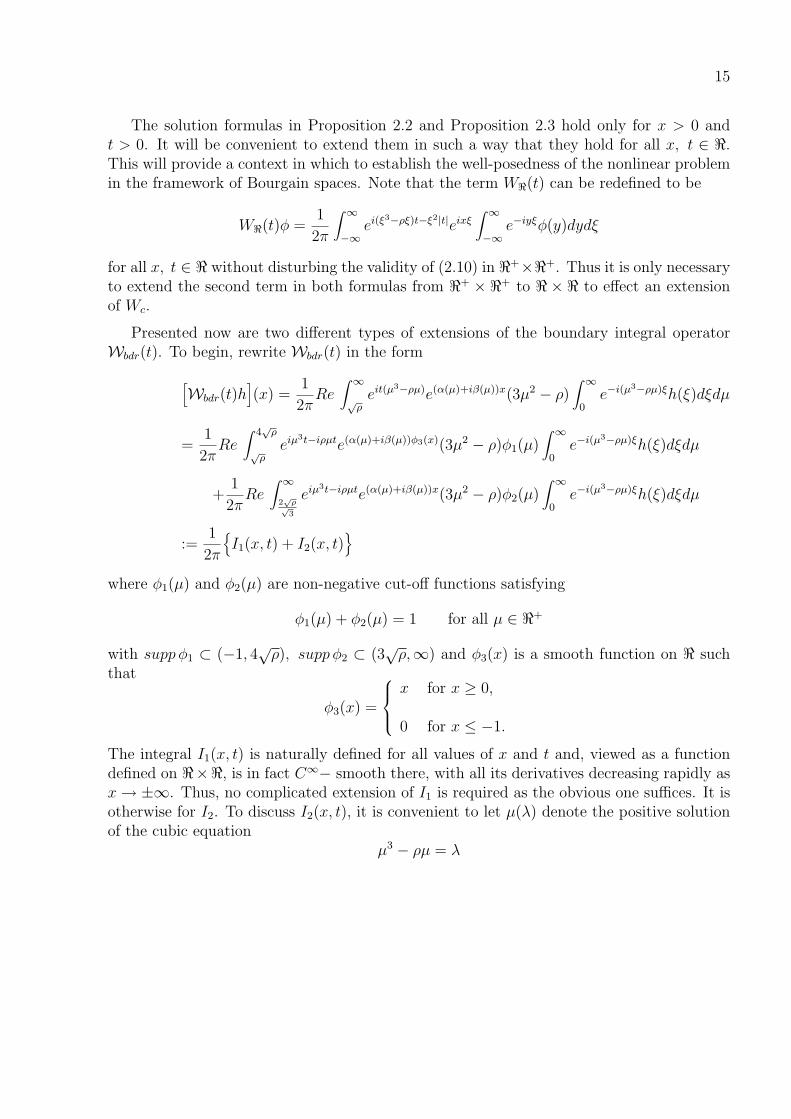
The solution formulas in Proposition 2.2 and Proposition 2.3 hold only for x > 0 andt > 0. It will be convenient to extend them in such a way that they hold for all x, t ∈ <.This will provide a context in which to establish the well-posedness of the nonlinear problemin the framework of Bourgain spaces. Note that the term W<(t) can be redefined to be

W<(t)φ =1

2π

∫ ∞

−∞ei(ξ3−ρξ)t−ξ2|t|eixξ

∫ ∞

−∞e−iyξφ(y)dydξ

for all x, t ∈ < without disturbing the validity of (2.10) in <+×<+. Thus it is only necessaryto extend the second term in both formulas from <+ × <+ to < × < to effect an extensionof Wc.

Presented now are two different types of extensions of the boundary integral operatorWbdr(t). To begin, rewrite Wbdr(t) in the form

[Wbdr(t)h

](x) =

1

2πRe

∫ ∞

√ρeit(µ3−ρµ)e(α(µ)+iβ(µ))x(3µ2 − ρ)

∫ ∞

0e−i(µ3−ρµ)ξh(ξ)dξdµ

=1

2πRe

∫ 4√

ρ

√ρ

eiµ3t−iρµte(α(µ)+iβ(µ))φ3(x)(3µ2 − ρ)φ1(µ)∫ ∞

0e−i(µ3−ρµ)ξh(ξ)dξdµ

+1

2πRe

∫ ∞

2√

ρ√3

eiµ3t−iρµte(α(µ)+iβ(µ))x(3µ2 − ρ)φ2(µ)∫ ∞

0e−i(µ3−ρµ)ξh(ξ)dξdµ

:=1

2π

I1(x, t) + I2(x, t)

where φ1(µ) and φ2(µ) are non-negative cut-off functions satisfying

φ1(µ) + φ2(µ) = 1 for all µ ∈ <+

with supp φ1 ⊂ (−1, 4√ρ), supp φ2 ⊂ (3

√ρ,∞) and φ3(x) is a smooth function on < such

that

φ3(x) =

x for x ≥ 0,

0 for x ≤ −1.

The integral I1(x, t) is naturally defined for all values of x and t and, viewed as a functiondefined on <×<, is in fact C∞− smooth there, with all its derivatives decreasing rapidly asx→ ±∞. Thus, no complicated extension of I1 is required as the obvious one suffices. It isotherwise for I2. To discuss I2(x, t), it is convenient to let µ(λ) denote the positive solutionof the cubic equation

µ3 − ρµ = λ

16

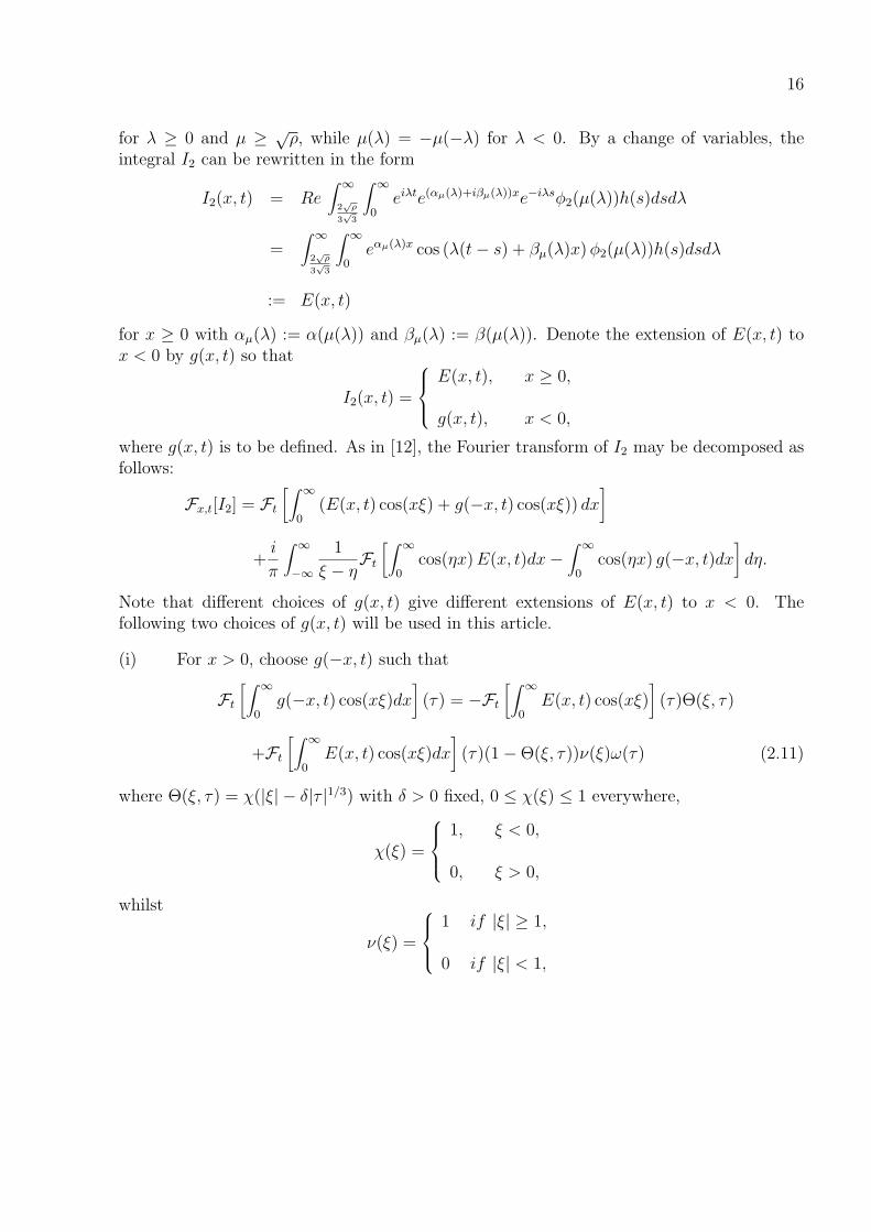
for λ ≥ 0 and µ ≥ √ρ, while µ(λ) = −µ(−λ) for λ < 0. By a change of variables, the

integral I2 can be rewritten in the form

I2(x, t) = Re∫ ∞

2√

ρ

3√

3

∫ ∞

0eiλte(αµ(λ)+iβµ(λ))xe−iλsφ2(µ(λ))h(s)dsdλ

=∫ ∞

2√

ρ

3√

3

∫ ∞

0eαµ(λ)x cos (λ(t− s) + βµ(λ)x)φ2(µ(λ))h(s)dsdλ

:= E(x, t)

for x ≥ 0 with αµ(λ) := α(µ(λ)) and βµ(λ) := β(µ(λ)). Denote the extension of E(x, t) tox < 0 by g(x, t) so that

I2(x, t) =

E(x, t), x ≥ 0,

g(x, t), x < 0,

where g(x, t) is to be defined. As in [12], the Fourier transform of I2 may be decomposed asfollows:

Fx,t[I2] = Ft

[∫ ∞

0(E(x, t) cos(xξ) + g(−x, t) cos(xξ)) dx

]

+i

π

∫ ∞

−∞

1

ξ − ηFt

[∫ ∞

0cos(ηx)E(x, t)dx−

∫ ∞

0cos(ηx) g(−x, t)dx

]dη.

Note that different choices of g(x, t) give different extensions of E(x, t) to x < 0. Thefollowing two choices of g(x, t) will be used in this article.

(i) For x > 0, choose g(−x, t) such that

Ft

[∫ ∞

0g(−x, t) cos(xξ)dx

](τ) = −Ft

[∫ ∞

0E(x, t) cos(xξ)

](τ)Θ(ξ, τ)

+Ft

[∫ ∞

0E(x, t) cos(xξ)dx

](τ)(1−Θ(ξ, τ))ν(ξ)ω(τ) (2.11)

where Θ(ξ, τ) = χ(|ξ| − δ|τ |1/3) with δ > 0 fixed, 0 ≤ χ(ξ) ≤ 1 everywhere,

χ(ξ) =

1, ξ < 0,

0, ξ > 0,

whilst

ν(ξ) =

1 if |ξ| ≥ 1,

0 if |ξ| < 1,

17

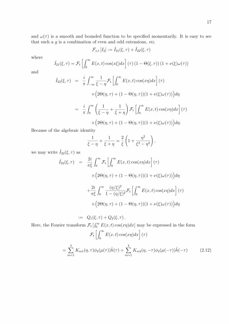
and ω(τ) is a smooth and bounded function to be specified momentarily. It is easy to seethat such a g is a combination of even and odd extensions, viz.

Fx,t [I2] := I21(ξ, τ) + I22(ξ, τ)

where

I21(ξ, τ) = Ft

[∫ ∞

0E(x, t) cos(xξ)dx

](τ) (1−Θ(ξ, τ)) (1 + ν(ξ)ω(τ))

and

I22(ξ, τ) =i

π

∫ ∞

−∞

1

ξ − ηFt

[∫ ∞

0E(x, t) cos(xη)dx

](τ)

×(2Θ(η, τ) + (1−Θ(η, τ))(1 + ν(ξ)ω(τ))

)dη

=i

π

∫ ∞

0

(1

ξ − η+

1

ξ + η

)Ft

[∫ ∞

0E(x, t) cos(xη)dx

](τ)

×(2Θ(η, τ) + (1−Θ(η, τ))(1 + ν(ξ)ω(τ))

)dη.

Because of the algebraic identity

1

ξ − η+

1

ξ + η=

2

ξ

(1 +

η2

ξ2 − η2

),

we may write I22(ξ, τ) as

I22(ξ, τ) =2i

πξ

∫ ∞

0Ft

[∫ ∞

0E(x, t) cos(xη)dx

](τ)

×(2Θ(η, τ) + (1−Θ(η, τ))(1 + ν(ξ)ω(τ))

)dη

+2i

πξ

∫ ∞

0

(η/ξ)2

1− (η/ξ)2Ft

[∫ ∞

0E(x, t) cos(xη)dx

](τ)

×(2Θ(η, τ) + (1−Θ(η, τ))(1 + ν(ξ)ω(τ))

)dη

:= Q1(ξ, τ) +Q2(ξ, τ) .

Here, the Fourier transform Ft [∫∞0 E(x, t) cos(xη)dx] may be expressed in the form

Ft

[∫ ∞

0E(x, t) cos(xη)dx

](τ)

=4∑

m=1

Km1(η, τ)φ2(µ(τ))h(τ) +4∑

m=1

Km2(η,−τ)φ2(µ(−τ))h(−τ) (2.12)

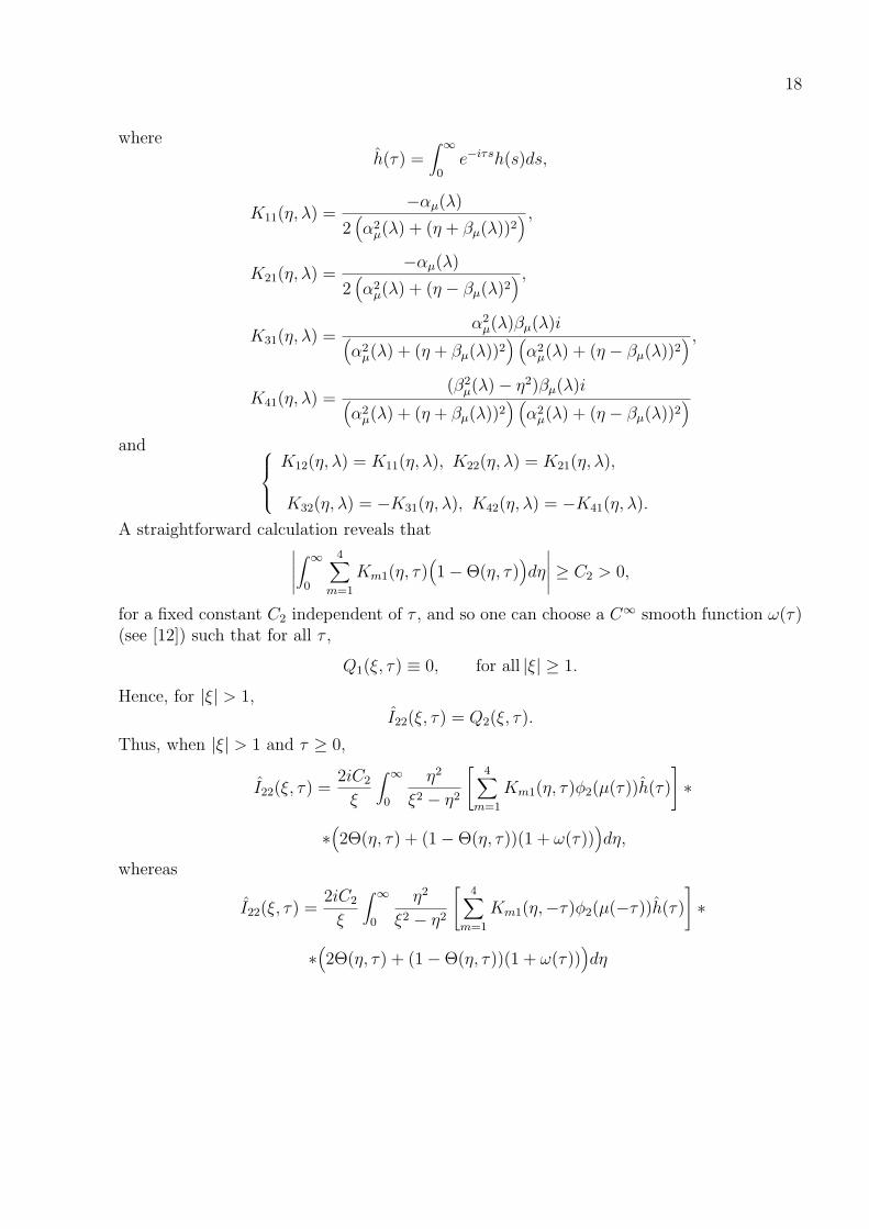
18

whereh(τ) =

∫ ∞

0e−iτsh(s)ds,

K11(η, λ) =−αµ(λ)

2(α2

µ(λ) + (η + βµ(λ))2) ,

K21(η, λ) =−αµ(λ)

2(α2

µ(λ) + (η − βµ(λ)2) ,

K31(η, λ) =α2

µ(λ)βµ(λ)i(α2

µ(λ) + (η + βµ(λ))2) (α2

µ(λ) + (η − βµ(λ))2) ,

K41(η, λ) =(β2

µ(λ)− η2)βµ(λ)i(α2

µ(λ) + (η + βµ(λ))2) (α2

µ(λ) + (η − βµ(λ))2)

and K12(η, λ) = K11(η, λ), K22(η, λ) = K21(η, λ),

K32(η, λ) = −K31(η, λ), K42(η, λ) = −K41(η, λ).

A straightforward calculation reveals that∣∣∣∣∣∫ ∞

0

4∑m=1

Km1(η, τ)(1−Θ(η, τ)

)dη

∣∣∣∣∣ ≥ C2 > 0,

for a fixed constant C2 independent of τ , and so one can choose a C∞ smooth function ω(τ)(see [12]) such that for all τ ,

Q1(ξ, τ) ≡ 0, for all |ξ| ≥ 1.

Hence, for |ξ| > 1,I22(ξ, τ) = Q2(ξ, τ).

Thus, when |ξ| > 1 and τ ≥ 0,

I22(ξ, τ) =2iC2

ξ

∫ ∞

0

η2

ξ2 − η2

[4∑

m=1

Km1(η, τ)φ2(µ(τ))h(τ)

]∗

∗(2Θ(η, τ) + (1−Θ(η, τ))(1 + ω(τ))

)dη,

whereas

I22(ξ, τ) =2iC2

ξ

∫ ∞

0

η2

ξ2 − η2

[4∑

m=1

Km1(η,−τ)φ2(µ(−τ))h(τ)]∗

∗(2Θ(η, τ) + (1−Θ(η, τ))(1 + ω(τ))

)dη

19

when |ξ| ≥ 1 and τ < 0. The boundary integral operator corresponding to this extension ofWbdr(t) is denoted by BI1(t).

(ii) Choose g(−x, t) such that

Ft

[∫ ∞

0g(−x, t) cos(xξ)dx

](τ) = −Ft

[∫ ∞

0E(x, t) cos(xξ)

](τ)(1−Θ(ξ, τ))

+Ft

[∫ ∞

0E(x, t)cos(xξ)dx

](τ)Θ(ξ, τ)ν(ξ)ω(τ) (2.13)

where Θ is as before. In this case, we have

Fx,t [I2] := I∗21(ξ, τ) + I∗22(ξ, τ)

with

I∗21(ξ, τ) = Ft

[∫ ∞

0E(x, t) cos(xξ)dx

]Θ(ξ, τ) (1 + ν(ξ)ω(τ))

and

I∗22(ξ, τ) =i

π

∫ ∞

−∞

1

ξ − ηFt

[∫ ∞

0E(x, t) cos(xη)dx

]∗

∗(2 (1−Θ(η, τ)) + Θ(η, τ)(1 + ν(ξ)ω(τ))

)dη

=i

π

∫ ∞

0

(1

ξ − η+

1

ξ + η

)Ft

[∫ ∞

0E(x, t) cos(xη)dx

]∗

∗(2(1−Θ(η, τ)) + Θ(η, τ)(1 + ν(ξ)ω(τ))

)dη

=2iC2

ξ

∫ ∞

0Ft

[∫ ∞

0E(x, t) cos(xη)dx

]∗

∗(2(1−Θ(η, τ)) + Θ(η, τ)(1 + ν(ξ)ω(τ))

)dη

+2iC2

ξ

∫ ∞

0

(η/ξ)2

1− (η/ξ)2Ft

[∫ ∞

0E(x, t) cos(xη)dx

]∗

∗(2(1−Θ(η, τ)) + Θ(η, τ)(1 + ν(ξ)ω(τ))

)dη

:= Q∗1(ξ, τ) +Q∗

2(ξ, τ).

20

As in case (ii), one can choose an appropriate ω(τ) so that

Q∗1(ξ, τ) = 0 for |ξ| > 1 and any τ ∈ <.

The boundary integral operator corresponding to this extension of Wbdr(t) is denoted byBI2(t).

2.2 Linear estimates

In this subsection, estimates are provided for solutions of the associated linear versionof the KdV-Burgers equation. These are needed in establishing the well-posedness of thenonlinear problems in the next section.

For given s ∈ <, 0 ≤ b ≤ 1 and any measurable function w ≡ w(x, t) : < × < → <,define

Λs,b(w) =(∫ ∞

−∞

∫ ∞

−∞

⟨i(τ − (ξ3 − ρξ)) + ξ2

⟩2b< ξ >2s |w(ξ, τ)|2 dξdτ

)1/2

(2.14)

where < · >= (1 + | · |2)1/2. Let Xs,b be the completion of the space of all functions wsatisfying

‖w‖Xs,b:= Λs,b(w) <∞

and letXs,b ≡ C(<;Hs(<)) ∩Xs,b

with the norm

‖w‖Xs,b=

(supt∈<

‖w(·, t)‖2Hs(<) + ‖w‖2

Xs,b

)1/2

.

First, consider the semigroup W<(t)t≥0 associated to the linear KdV-Burgers equationposed on the whole line <. Recall that for any φ ∈ S ′, the space of tempered distributions,and t ≥ 0,

Fx(W<(t)φ)(ξ) = exp[−ξ2t+ i(ξ3 − ρξ)t

]φ(ξ).

Extend W< to a linear operator defined on the whole real axis by setting

Fx(W<(t)φ)(ξ) = exp[−ξ2|t|+ i(ξ3 − ρξ)t

]φ(ξ)

for all t ∈ <. The proof of the following proposition regarding W<(t)∞0 is a minor modifi-cation of arguments found in [49].

Proposition 2.4 Let s ∈ <, 0 < b ≤ 1 and 0 < δ < 12

be given. Let ψ be a C∞ smoothfunction with compact support.

21

(i) There exists a constant C depending only on s, b and ψ such that

‖ψ(t)W<(t)φ‖Xs,b≤ C ‖φ‖Hs(<) . (2.15)

(ii) There exists Cδ such that for all u ∈ Xs,− 12+δ,∥∥∥∥ψ(t)

∫ t

0W<(t− t′)f(t′)dt′

∥∥∥∥X

s, 12

≤ Cδ ‖f‖Xs,− 1

2+δ. (2.16)

(iii) There exists a constant C depending only on s such that

supx∈<

‖W<(t)φ‖H

s3t (<)

≤ C ‖φ‖Hs(<) . (2.17)

(iv) For all f ∈ Xs,− 12+δ, the correspondence

t 7→∫ t

0W<(t− t′)f(t′)dt′

lies in C(<+, Hs+2δ(<)). In addition, if fn is a sequence with fn → 0 in Xs,− 12+δ,

then ∥∥∥∥∫ t

0W<(t− t′)fn(t′)dt′

∥∥∥∥L∞(<+,Hs+2δ(<))

→ 0 as n→∞.

Next, attention is turned to the spatial traces of W<(t)φ and∫ t0 W<(t− t′)f(·, t′)dt.

Proposition 2.5 Let s ∈ [−1, 5] be given. There exists a constant C depending only on ssuch that

supx∈<

‖W<(t)φ‖H

s+13

t (<)≤ C‖φ‖Hs(<) (2.18)

andsupx∈<

‖∂xW<(t)φ‖H

s3t (<)

≤ C‖φ‖Hs(<) (2.19)

for any φ ∈ Hs(<).

The proof of this proposition is based on the following technical lemma which plays thesame role in our arguments as would a Plancherel Theorem. The proof of the lemma ispostponed and provided in Appendix II.

22

Lemma 2.6 Suppose 0 < ν < 1 and let I be the integral operator defined by

[I(f)](t) :=∫ ∞

−∞eitη+µ(η)|t|f(η)dη, for t ∈ <,

where µ : < → (−∞, 0] is continuous function satisfying

|µ(η)| ∼ ην as η → 0 and |µ(η)| ∼ |η|13 as |η| → ∞.

Then, I is a bounded linear operator on L2(<), which is to say, there exists a constant Csuch that

‖I(f)‖L2(<) ≤ C ‖f‖L2(<)

for all f ∈ L2(<).

Proof of Proposition 2.5: We only provide the proof of (2.18). The proof of (2.19) is verysimilar and is therefore omitted. Let u(x, t) = W<(t)φ. Then, a change of variables revealsthat

u(x, t) =∫ ∞

−∞eixξe[i(ξ

3−ρξ)]t−ξ2|t|φ(ξ)dξ

=∫|λ|≥√ρ

eixν(λ)eiλt−ν2(λ)|t|(3ν2(λ)− ρ)−1φ(ν(λ))dλ,

where ξ = ν(λ) solves the equationξ3 − ρξ = λ

with ν(λ) ∼ λ13 as λ→∞. By Lemma 2.6,

‖u(x, ·)‖L2(<) ≤ C(∫ ∞

−∞

∣∣∣(3ν2(λ)− ρ)−1φ(ν(λ))∣∣∣2 dλ) 1

2

≤ C ‖φ‖H−1(<)

for any x ∈ <. Note that

ut(x, t) =∫ ∞

−∞eixξe[i(ξ

3−ρξ)]t−ξ2|t|[i(ξ3 − ρξ) + κ(t)ξ2]φ(ξ)dξ,

where κ(t) = −1 if t ≥ 0 and κ(t) = 1 if t < 0. Applying Lemma 2.6 again yields that

‖u(x, ·)‖H1(<) ≤ C ‖φ‖H2(<)

for any x ∈ <. Similarly, one can show that

‖u(x, ·)‖H2(<) ≤ C ‖φ‖H5(<)

for any x ∈ <. The inequality (2.18) then follows by interpolation. The proof is therebycompleted. 2

23

Proposition 2.7 Let 0 ≤ b < 1/2, −1 ≤ s ≤ 2− 3b, ψ ∈ C∞0 (<) and

w(x, t) =∫ t

0W<(t− t′)f(·, t′)dt′.

Then, there exists C depending only on b, s and ψ such that

supx∈<

‖ψ(·)w(x, ·)‖H

s+13

t (<)≤ C ‖f‖Xs,−b

(2.20)

andsupx∈<

‖ψ(t)wx(x, t)‖Hs/3t (<)

≤ C ‖f‖Xs,−b. (2.21)

Proof: The proof presented below is based on the approach developed in [15, 44], appropri-ately modified. As the proof of (2.21) is similar to that of (2.20), only (2.20) is proved.

First, observe that

ψ(t)∫ t

0W<(t− t′)f(t′)dt′

= ψ(t)∫ ∞

−∞

∫ ∞

−∞eixξf(ξ, τ)ψ(|τ − (ξ3 − ρξ)|+ ξ2)

eiτt − eit(ξ3−ρξ)−ξ2t

i[τ − (ξ3 − ρξ)] + ξ2dξdτ

+ψ(t)∫ ∞

−∞

∫ ∞

−∞eixξf(ξ, τ)(1− ψ(|τ − (ξ3 − ρξ))|+ ξ2))

eiτt − eit(ξ3−ρξ)−ξ2t

i[τ − (ξ3 − ρξ)] + ξ2dξdτ

:= A+B.

By a Taylor series expansion, we see that

A =∞∑

k=1

1

k!ψk(t)W<(t)g

withg(ξ) =

∫ ∞

−∞f(ξ, τ)(i(τ − (ξ3 − ρξ)) + ξ2)k−1ψ(|τ − (ξ3 − ρξ))|+ ξ2)dτ

andψk(t) := tkψ(t), k = 1, 2, · · · .

Note that‖ψk‖

Hs+13 (<)

≤∫ ∞

−∞

∣∣∣ψk(τ)∣∣∣2 (1 + |τ |)2 s+1

3 dτ ≤ C(k + 1)2

24

and

‖g‖2Hs(<) ≤ C

∫ ∞

−∞〈ξ〉2s

∣∣∣∣∫ ∞

−∞f(ξ, τ)(i(τ − (ξ3 − ρξ)) + ξ2)k−1ψ(|τ − (ξ3 − ρξ)|+ ξ2)dτ

∣∣∣∣2 dξ≤ C

∫ ∞

−∞〈ξ〉2s

∣∣∣∣∣∫|τ−(ξ3−ρξ)|+ξ2<1

f(ξ, τ)dτ

∣∣∣∣∣2

dξ

≤ C∫ ∞

−∞〈ξ〉2s

∣∣∣∣∣∫ ∞

−∞

f(ξ, τ)

1 + |τ − (ξ3 − ρξ)|+ ξ2dτ

∣∣∣∣∣2

dξ

because of the restriction on the support of ψ. Thus, applying (2.20) gives

supx∈<

‖A(x, ·)‖H

s+13

t (<)≤ C

∞∑k=1

(k + 1)2

k!‖g‖Hs(<)

≤ C

∫ ∞

−∞〈ξ〉2s

∣∣∣∣∣∫ ∞

−∞

f(ξ, τ)

1 + |τ − (ξ3 − ρξ)|+ ξ2dτ

∣∣∣∣∣2

dξ

12

≤ C‖f‖Xs,−b

because 0 ≤ b < 12.

Next, consider the term B which can be written

B = B1 +B2

with

B1 = −ψ(t)∫ ∞

−∞ei(xξ+t(ξ3−ρξ))−ξ2t

(∫ ∞

−∞

1− ψ(|τ − (ξ3 − ρξ)|+ ξ2)

i(τ − (ξ3 − ρξ)) + ξ2f(ξ, τ)

)dξ

and

B2 = ψ(t)∫ ∞

−∞ei(xξ+tτ)−ξ2t

(∫ ∞

−∞

1− ψ(|τ − (ξ3 − ρξ)|+ ξ2)

i(τ − (ξ3 − ρξ)) + ξ2f(ξ, τ)

)dξ.

For B1, Proposition 2.6 yields

supx∈R

‖B1(x, t)‖2

Hs+12

t (R)≤ C

∫ ∞

−∞〈ξ〉2s

(∫ ∞

−∞

|f(ξ, τ)|(1 + |τ − (ξ3 − ρξ)|+ ξ2

dτ

)2

dξ ≤ C‖f‖2Xs,−b

.

25

As for B2(x, t),

supx∈R

‖B2(x, t)‖2

Hs+13

t (<)

≤ C∫ ∞

−∞(1 + |τ |)

2(s+1)3

(∫ ∞

−∞

|1− ψ(|τ − (ξ3 − ρξ)|+ ξ2)||τ − (ξ3 − ρξ)|+ ξ2

f(ξ, τ)dξ

)2

dτ

≤ C∫ ∞

−∞(1 + |τ |)

2(s+1)3

(∫ ∞

−∞

1

1 + |τ − (ξ3 − ρξ)|+ ξ2f(ξ, τ)dξ

)2

dτ

≤ C∫ ∞

−∞(1 + |τ |)

2(s+1)3 G(τ)

∫ ∞

−∞

|f(ξ, τ)|2 〈ξ〉2s

(1 + |τ − (ξ3 − ρξ)|+ ξ2)2bdξdτ

where

G(τ) :=∫ ∞

−∞

dξ

〈ξ〉2s (1 + |τ − (ξ3 − ρξ)|+ ξ2)2(1−b)

≤ C∫ ∞

−∞

dη

|η| 23 (1 + |η|) 2s3 (1 + |τ − η|)2(1−b)

.

Therefore, it suffices to show that there exists a constant C such that for any τ ∈ <,

G(τ) ≤ C

(1 + |τ |)2(s+1)

3

. (2.22)

To see this true, write G(τ) as

G(τ) = G1(τ) +G2(τ) +G3(τ)

with

G1(τ) =∫|η|≤ 1

2|τ |

dη

|η| 23 (1 + |η|) 2s3 (1 + |τ − η|)2(1−b)

,

G2(τ) =∫|τ |/2<|η|<2|τ |

dη

|η| 23 (1 + |η|) 2s3 (1 + |τ − η|)2(1−b)

and

G3(τ) =∫2|τ |≤|η|

dη

|η| 23 (1 + |η|) 2s3 (1 + |τ − η|)2(1−b)

.

26

In the region 2|η| ≤ |τ |, note that (1 + |τ − η|) ≥ 12(1 + |τ |) and |τ − η| ≥ 1

2|η|. Thus, for

s ≤ 0,

G1(τ) ≤ C(1 + |τ |)−2(s+1)

3

∫ ∞

−∞

dη

|η| 23 (1 + |η|)2(1−b)− 23

≤ C

(1 + |τ |)2(s+1)

3

as b < 12. When 0 ≤ s ≤ 2− 3b,

G1(τ) ≤ C(1 + |τ |)−2(s+1)

3

∫ ∞

−∞

dη

|η| 23 (1 + |η|) 2s3 (1 + |τ − η|)2(1−b)− 2(s+1)

3

≤ C(1 + |τ |)−2(s+1)

3

∫ ∞

−∞

dη

|η| 23 (1 + |η|)2(1−b)− 23

≤ C

(1 + |τ |)2(s+1)

3

.

In the region |τ |/2 < |η| < 2|τ |,

G2(τ) ≤ C(1 + |τ |)−2(s+1)

3

∫ 2|τ |

|τ |/2

dη

(1 + |τ − η|)2(1−b)

≤ C

(1 + |τ |)2 s+13

,

again because b < 1/2. In the region 2|τ | ≤ |η|, it is the case that 1 + |τ − η| = O(1 + |η|).Thus, it transpires that

G3(τ) ≤ C∫|η|≥2|τ |

dη

|η|2(s+1)

3 (1 + |η|)2(1−b)

≤ C(1 + |τ |)−2(s+1)

3 .

The inequality (2.20) has therefore been established for −1 ≤ s ≤ 2 − 3b. This completesthe proof. 2

Finally, attention is focused upon the boundary integral operators BI1(t) and BI2(t).

Proposition 2.8 Let ψ ∈ C∞0 (<) be given and assume that 0 ≤ b < 1

2− s

3with s ≤ 0. Then

there exists a constant C such that

‖ψBI1(h)‖Xs,b≤ C ‖h‖

H3b+s−1/2

3 (<+)(2.23)

for any h ∈ H3b+s−1/2

30 (<+).

27

Proposition 2.9 Let ψ ∈ C∞0 (<) be given and assume that 0 ≤ b < 5

6− s

3with −1

2< s < 1.

Then there exists a constant C such that

‖ψBI2(h)‖Xs,b≤ C ‖h‖

H3b+s−1/2

3 (<+)(2.24)

for any h ∈ H3b+s−1/2

30 (<+).

Proposition 2.10 Let −32< α < 1

2and −1

2< β < 1 be given. There exist constant Cα and

Cβ such thatsupt∈R

‖BI1h‖Hα(<) ≤ Cα ‖h‖H

α+13 (<+)

(2.25)

andsupt∈R

‖BI2h‖Hβ(<) ≤ Cβ ‖h‖H

β+13 (<+)

. (2.26)

Observe that‖w‖L2(0,T ;Hs(<)) ≤ CΛs,b(ψw)

for any s ∈ < and b ≥ 0, if ψ ∈ C∞0 (<) and ψ(t) = 1 when t ∈ (0, T ). The following result,

which follows from Proposition 2.8 and Proposition 2.9, presents a boundary smoothingproperty of the linear KdV-Burgers equation, which is same as that obtained for the linearKdV equation in [12].

Corollary 2.11 For any given T > 0 and s ≥ −32, there exists a constant C such that

‖Wbdrh‖L2(0,T ;Hs+3

2 (<+))≤ C ‖h‖

H1+s3 (<+)

(2.27)

for any h ∈ H1+s3

0 (<+).

The boundary integral operator Wbdr also possesses the sharp Kato smoothing property,the final result of this section.

Proposition 2.12 For any given T > 0 and s ≥ −32, there exists a constant C such that

supx∈<+

‖∂xWbdrh‖H

s3t (<+)

≤ C ‖h‖H

s+13 (<+)

(2.28)

for any h ∈ H1+s3

0 (<+).

The proofs of Propositions 2.8, 2.9 and 2.10 are similar to the results proved in Section 3 of[12]. A sketch of the proofs of Proposition 2.8 and Proposition 2.9 is provided in Appendix Ifor the reader’s convenience. As for Proposition 2.12, its proof is the same as the analogousresult in [12] and is therefore omitted.

28

3 Well-posedness

In this section, we study the well-posedness of the IBVP

ut + ρux + γuux + a1(x)b1(t)uux + a2(x)b2(t)u2 + uxxx − uxx = 0, x, t > 0,

u(x, 0) = φ(x), x ≥ 0,

u(0, t) = h(t), t ≥ 0,

(3.1)

where ρ > 0 and γ ∈ R are constants, aj ∈ H∞(<+) and bj ∈ C∞(<+) for j = 1, 2.

As mentioned earlier, for given s ∈ < and 0 ≤ b ≤ 1, Xs,b is the space of all functions wsatisfying

‖w‖Xs,b:= Λs,b(w) <∞

(see (2.14)) andXs,b ≡ C(R;Hs(R)) ∩Xs,b.

In addition, for given T > 0, Let Ds,T be the space of all function pairs (φ, h) ∈ Hs(<+) ×H

s+13 (0, T ) which is s−compatible with respect to the IBVP (3.1) with its norm inherited

from the space Hs(<+)×Hs+13 (0, T ), i.e.,

‖(φ, h)‖Ds,T:= ‖(φ, h)‖

Hs(<+)×Hs+13 (0,T )

for any (φ, h) ∈ Ds,T . Let Ys,b be the space of all functions w in Xs,b satisfying

supx∈<

‖wx(x, ·)‖H

s3t (<)

< +∞.

For any w ∈ Ys,b, define

‖w‖Ys,b=

(‖w‖2

Xs,b+ sup

x∈<‖wx(x, ·)‖2

Hs3t (<)

) 12

.

These Bourgain-type spaces are defined for functions whose domain is the whole plane<×<. However, the IBVP (3.1) is posed on the quarter plane <+ ×<+ and we are seekingits solution in the space C(<+ : Hs(<+)) corresponding to a given initial value in the space

Hs(<+) and boundary data in the space Hs+13

loc (<+). It is thus natural to consider restrictedversions of the these Bourgain-type spaces to the quarter plane <+ × <+. Let Ω denote asubinterval of <; define a Bourgain space Xs,b restricted to the domain <+ × Ω as follows:

Xs,b(<+ × Ω) = Xs,b|<+×Ω

29

with the quotient norm

‖u‖Xs,b(<+×Ω) ≡ infw∈Xs,b

‖w‖Xs,b: w(x, t) = u(x, t) on <+ × Ω.

The spaces Xs,b(<+ × Ω) and Ys,b(<+ × Ω) are defined similarly.For the IBVP (3.1), the following well-posedness result obtains.

Theorem 3.1 Let s ∈ (−1, 12) and r > 0 be given. There exists T with T > 0 such that for

a given pair (φ, h) ∈ Ds,T satisfying

‖(φ, h)‖Ds,T≤ r,

the IBVP (3.1) admits a unique solution u ∈ Ys, 12(<+ × (0, T )). Moreover, the solution u

depends Lipschitz continuously on (φ, h) in the corresponding spaces.

The proof of Theorem 3.1 is based on the results in Section 2 and the following lemmas.

Consider the non-homogeneous linear problem

ut + ρux − uxx + uxxx = 0, for x, t ≥ 0,

u(x, 0) = 0, u(0, t) = h(t).

(3.2)

Recall its solution may be written in the form

u(x, t) = [Wbdr(t)h] (x)

for x, t ≥ 0, as expounded in Section 2.

Lemma 3.2 For a given pair (b, s) satisfying

0 ≤ b < 12− s

3if s ≤ 0,

0 ≤ b < 56− s

3if −1

2< s < 1,

b = 12

if 1 ≤ s ≤ 3,

(3.3)

there exists a constant C such that for any T > 0 and any h ∈ Hs+13

0 (0, T ), the correspondingsolution u of (3.2) belongs to the restricted Bourgain space Ys,b(<+ × (0, T )) and satisfies

‖u‖Xs,b(<+×(0,T )) ≤ C ‖h‖H

3b+s−1/23 (0,T )

, (3.4)

‖u‖Xs, 12

(<+×(0,T )) ≤ C ‖h‖H

s+13 (0,T )

(3.5)

and‖u‖Ys,1/2(<+×(0,T )) ≤ C ‖h‖

Hs+13 (0,T )

. (3.6)

30

Proof: For T > 0, let h1 ∈ Hs+13 (<+) such that h1 ≡ h in the space H

s+13 (0, T ) and let

ψ1 ∈ C∞0 (R) be such that ψ1(t) = 1 for all t ∈ [0, T ]. Define

u1(x, t) =

[BI1(t)h1](x) if 0 ≤ b < 1

2− s

3and s < 0,

[BI2(t)h1](x) if 0 ≤ b < 56− s

3and 0 ≤ s < 1.

Observing thatu(x, t) = u1(x, t) for (x, t) ∈ <+ × [0, T ],

and using Proposition 2.8, Proposition 2.9 and Proposition 2.10, one arrives at the inequal-ities

‖u‖Xs, 12

(<+×(0,T )) ≤ ‖ψ1u1‖Xs, 12

≤ C ‖h1‖H

s+13 (<+)

from which (3.5) with −1 < s < 1 follows. In particular,

‖u‖X0, 12

(<+×(0,T )) ≤ C ‖h‖H

13 (<+)

. (3.7)

When 1 ≤ s ≤ 3, let v = ut. Then v solves

vt + ρvx − vxx + vxxx = 0, for x, t ≥ 0,

v(x, 0) = 0, v(0, t) = h′(t).

Thus

‖v‖X0, 12

(<+×(0,T )) ≤ C ‖h′‖H

13 (<+)

≤ c ‖h‖H

43 (<+)

.

Since v = ut = −ρux + uxx − uxxx, it follows that

‖u‖X3, 12

(<+×(0,T )) ≤ C ‖h‖H

43 (<+)

. (3.8)

The inequality (3.5) with 1 ≤ s ≤ 3 follows by interpolation of the estimates (3.14) and(3.8). The proof is complete. 2

Consider the same linear equation posed with zero boundary conditions, but non-trivialinitial data, viz.

ut + ρux − uxx + uxxx = 0, for x, t ≥ 0,

u(x, 0) = φ(x), u(0, t) = 0 .

(3.9)

As mentioned earlier, its solution can be written as

u(x, t) = [Wc(t)φ] (x)

for x, t ≥ 0.

31

Lemma 3.3 For a given s ∈ (−1, 12), there exists a constant C such that for any T > 0 and

any φ ∈ Hs0(<+), the corresponding solution u of (3.9) belongs to the restricted Bourgain

space Ys, 12(<+ × (0, T )) and satisfies the inequality

‖u‖Ys, 12

(<+×(0,T )) ≤ C ‖φ‖Hs(<+) . (3.10)

Proof: According to Proposition 2.2, one may write Wc(t)φ as

Wc(t)φ = W<(t)φ∗ −Wbdr(t)g

for any x, t > 0, where g is the trace of W<(t)φ∗ at x = 0, φ∗ ∈ Hs(<) and φ∗ equals φwhen restricted on <+. The estimate (3.10) follows from Proposition 2.4, Proposition 2.5and Lemma 3.2. 2

We turn now to consideration of the forced linear problem

ut + ρux − uxx + uxxx = f, for x, t ≥ 0,

u(x, 0) = 0, u(0, t) = 0 .

(3.11)

Its solution can be written in the form

u(·, t) =∫ t

0Wc(t− τ)f(·, τ)dτ.

Lemma 3.4 Assume that −1 < s ≤ 3− 2b and 0 < b < 12. There exists a constant C such

that for any T > 0 and any f ∈ Xs,−b(<+ × (0, T )), the corresponding solution u of (3.11)belongs to the space Xs,1/2(<+ × (0, T )) and satisfies the estimate

‖u‖Ys, 12

(<+×(0,T )) ≤ C ‖f‖Xs,−b(<+×(0,T )) . (3.12)

Proof: By Proposition 2.3,

u(·, t) =∫ t

0W<(t− τ)f(·, τ)dτ −Wbdr(t)v

for any x, t > 0 where v ≡ v(t) is the trace of∫ t0 W<(t− τ)f(·, τ)dτ at x = 0. The estimate

(3.12) then follows from Proposition 2.4, Proposition 2.7 and Lemma 3.2. 2

The next lemma presents a version of so-called bilinear estimates in the restricted Bour-gain space Xs,b(<+ × (0, T )) which follows directly from Lemma 3.1 in [49].

Lemma 3.5 Given s > −1 and T > 0, there exist positive constants C, µ, δ such that

‖∂x(uv)‖Xs,−1/2+δ(<+×(0,T )) ≤ CT µ ‖u‖Xs,1/2(<+×(0,T )) ‖v‖Xs,1/2(<+×(0,T )) (3.13)

for any u, v ∈ Xs,1/2(<+ × (0, T )).

32

We are now prepared to present a proof of Theorem 3.1.

Proof of Theorem 3.1: By applying Lemmas 3.2–3.5, Theorem 3.1 can be established bythe standard contraction mapping principle.

Let φ ∈ Hs(<+) and h ∈ Hs+13

loc (<+) be given with s ∈ (−1, 12). For given θ with 0 < θ ≤ 1

(to be chosen precisely momentarily) and v, w ∈ Ys, 12(<+ × (0, θ)), define

F(w) = Wc(t)φ+Wbdr(t)h−∫ t

0Wc(t− τ)

(a1b1wxw + a2b2w

2)

(τ)dτ.

Using Lemma 3.2 -Lemma 3.5, it is seen that

‖F(w)‖Ys, 12

(<+×(0,θ)) ≤ C1

(‖φ‖Hs(<+) + ‖h‖

Hs+13 (0,T )

)+ C2θ

µ ‖w‖2Y

s, 12(<+×(0,θ))

and‖F(v)− F(w)‖Y

s, 12(<+×θ)) ≤ C2θ

µ ‖v − w‖Ys, 12

(<+×(0,θ)) ‖v + w‖Ys, 12

(<+×(0,θ))

where the constant C1 and C2 are independent of θ, v and w. Let Br be the ball centeredat the origin in the space Ys, 1

2(<+ × (0, θ)) with radius r where

r = 2C1

(‖φ‖Hs(<+) + ‖h‖

Hs+13 (0,θ)

),

and choose θ = T small enough that

2C2Tµr ≡ β < 1.

In this case, it follows readily that F maps Br into itself and that for w, v ∈ Br,

‖F(w)− F(v)‖Ys, 12

(<+×(0,T )) ≤ β ‖w − v‖Ys, 12

(<+×(0,T )) .

Thus, the mapping F is a contraction mapping of the ball Br. The fixed point u in Br ofthis map F is the advertised solution. 2

The well-posedness result presented in Theorem 3.1 is conditional since uniqueness isestablished in the space Ys, 1

2(<+×(0, T )) instead of in the space C([0, T ];Hs(<+)). However,

following the procedure developed in [11], one can show that in fact uniqueness holds in thespace C([0, T ];Hs(<+)).

Proposition 3.6 Let s ∈ (−1, 12) and r > 0 be given. There exists a T > 0 depending only

on s and r such that for a given (φ, h) ∈ Ds,T satisfying

‖φ‖Ds,T≤ r,

the IBVP (3.1) admits a unique solution u ∈ C([0, T ];Hs(<+)). Moreover, the solution udepends Lipscitz continuously in the space C([0, T ];Hs(<+)) on (φ, h) in the space Ds,T .

33

This well-posedness result can be extended to be valid for any s ≥ 12.

Theorem 3.7 Let s > −1 and r > 0 be given with s 6= 3m+ 12, m = 1, 2, · · ·. There exists

a T > 0 depending only on s and r such that for a given (φ, h) ∈ Ds,T satisfying

‖φ‖Ds,T≤ r,

the IBVP (3.1) admits a unique solution u ∈ C([0, T ];Hs(<+)). Moreover, the solution udepends Lipschitz continuously on (φ, h) in their respective spaces.

Proof: The proof is provided only for the case wherein 0 ≤ s ≤ 3. The proof of theremaining case is similar and so is omitted.

First note that according to Theorem 3.1, for given r0 > 0, there exists a T0 > 0 dependsonly on r0 such that if (φ, h) ∈ D0,T0 satisfying ‖(φ, h)‖D0,T0

≤ r0, the IBVP (3.1) admits aunique solution u ∈ Y0,T0 and

‖u‖Y0,T0≤ Cr0‖(φ, h)‖D0,T0

(3.14)

where Cr0 is a constant depends (continuously) only on r0. Morover, for any (φjhj) ∈ D0,T0

with ‖(φj, hj)‖D0,T0≤ r0 for j = 1, 2, their corresponding solutions uj (j = 1, 2) to the IBVP

(3.1) satisfy‖u1 − u2‖Y0,T0

≤ Cr0‖(φ1, h1)− (φ2, h2)‖D0,T0.

Next suppose given (φ, h) ∈ D3,T0 satisfying

‖(φ, h)‖D0,T0≤ r0.

Applying Theorem 3.1 gives a solution u ∈ Y0,T0 satisfying the estimate (3.14). We claimthis solution u, in fact, belongs to the space C([0, T0];H

3(<+)) and

‖u‖C([0,T0];H3(<+)) ≤ Cr0 ‖(φ, h)‖D3,T0.

To see this, let v = ut. Then v satisfies

vt + ρvx + (γ + a1b1)(uv)x + 2a2b2uv − vxx + vxxx = f, x, t ∈ <+,

v(x, 0) = φ1(x), v(0, t) = h1(t).

(3.15)

Here, f = −a1(x)b′1(t)uux−a2(x)b

′2(t)u

2, h1(t) = h′(t) and φ1 is defined as in (1.2). This is anIBVP for a linearized KdV-Burgers equation with variable coefficients. The same argumentas presented in support of Theorem 3.1 yields that there exists a T ′ ∈ (0, T0] such that the

IBVP (3.15) has a unique solution v ∈ Y0,T ′ since φ1 ∈ L2(<+) and h1 ∈ H13 (0, T0). This, in

turn, implies that u ∈ C([0, T ′];H3(<+)) since

v = ut = −uxxx + uxx − γuux − ρux − a1(x)b1(t)uux − a2(x)b2(t)u2.

34

Note that T ′ only depends on ‖u‖Y0,T0and is therefore only on r0 according to (3.14). So by

a standard co argument, one may extend T ′ so that T ′ = T0.Thus Theorem 3.7 holds for s = 0 and s = 3. To see it is also true for 0 < s < 3, for any

(φ, h) ∈ Ds,T0 , we define

Ir0(φ, h) =

(φ, h) if ‖(φ, h)‖D0,T0

≤ r0,

r‖(φ,h)‖D0,T0

(φ, h) if ‖(φ, h)‖D0,T0≥ r0.

Then the IBVP (3.1) well defines a nonlinear mapK fromDj,T0 to the space C([0, T ];Hj(<+))for j = 0, 3 by

K(φ, h) = u

with u be the solution of the IBVP (3.1) with (φ, h) replaced by Ir(φ, h). Moreover, K isLipschitz continuous from the space D0,T0 to the space C([0, T0];L

2(<+)) and there exists aconstant C∗ depending only on ‖(φ, h)‖D0,T)

such that

‖K(φ, h)‖C([0,T0];H3(<+)) ≤ C∗ ‖(φ, h)‖D0,T0

for any (φ, h) ∈ D3,T0 . Invoking the nonlinear interpolation theory [54], we see that theoperator K is also well defined from the space Ds,T0 to the space C([0, T0];H

s(<+)) for anys ∈ (0, 3). Thus, for any (φ, h) ∈ D∫ ,T′ with ‖(φ, h)‖D0,T0

≤ r0 with 0 < s < 3, one arrivesthat the corresponding solution u ∈ C([0, T ];Hs(<+)). 2

Next, we turn to the issue of global well-posedness of the IBVP (3.1). The argumentsused in [12] can be applied here to give the following global well-posedness result.

Theorem 3.8 Let s ≥ 0 and T > 0 be given with s 6= 3m + 12, m = 1, 2, · · ·. Assume that

the coefficients a1(x)b1(t) and a2(x)b2(t) in the system (3.1) satisfy

a2(x)b2(t) ≡1

3a′1(x)b1(t) for any t, x > 0. (3.16)

Then, for any s−compatible (φ, h) ∈ Hs(<+) × Hs+13

+η(s)

loc (<+), the IBVP (3.1) admits aunique solution u ∈ C([0, T ];Hs(<+)), where η(s) = 0 when s ≥ 3 and η(s) = ε when0 ≤ s < 3 for an arbitrarily small ε > 0. Moreover, the solution u depends analytically on φand h in their respective function classes.

Note that as a consequence of the assumption (3.16), the system (3.1) has the followingglobal a priori estimate: any smooth solution u of the IBVP (3.1) with boundary data h ≡ 0satisfies

sup0≤t≤T

‖u(·, t)‖L2(<+) ≡ ‖φ‖L2(<+) . (3.17)

35

When −1 < s < 0, Molinet and Ribaud [49] showed that the IVP for the KdV-Burgersequation is also globally well-posed in the space Hs(<) by taking the advantage of thedissipative term −uxx. We have a similar global well-posedness result for the IBVP (3.1).

Theorem 3.9 Assume that the coefficients a1(x)b1(t) and a2(x)b2(t) in the system (3.1)satisfy condition (3.16). Let −1 < s < 0 and T > 0 be given. For any given (φ, h) ∈

Hs(<+)×H1+

3loc (<+), the IBVP (3.1) admits a unique solution u ∈ C([0, T ];Hs(<+)). More-

over, for any ε > 0, this solution also lies in the class L2([ε, T ];H32 (<+)).

The following lemma is needed in the proof.

Lemma 3.10 Suppose to be given s > −1 and T > 0. There exists a δ > 0 such that for allu ∈ Xs, 1

2(<+ × (0, T )),

w =∫ t

0Wc(t− τ)(uux)(τ)dτ ∈ L2(0, T ;Hs+δ(<+)).

Proof: By Proposition 2.3, we may rewrite w as w = w1 + w2 with

w1 =∫ t

0W<(t− τ)(uux)(τ)dτ and w2 = Wbdr(t)g

where g is the trace of w1 at x = 0. According to Lemma 3.5, there exists a δ > 0 such thatuux ∈ Xs,− 1

2+δ(<+× (0, T )). Thus, w1 ∈ L2(0, T ;Hs+δ(<+)) by Proposition 2.4. In addition,

it follows from Proposition 2.5 that g ∈ H s+13 (<) which yields that w2 ∈ L2(0, T ;Hs+δ(<+))

by Corollary 2.11. The proof is complete. 2

Proof of Theorem 3.9: By Theorem 3.1, the IBVP (3.1) admits a unique solution

u ∈ C([0, T ∗];Hs(<+))

for some T ∗ ≤ T . Moreover, u can be decomposed in the form

u(x, t) = u1(x, t) + u2(x, t) + u3(x, t)

with

u1(x, t) = Wc(t)φ, u2(x, t) = Wbrd(t)h, u3(x, t) = −∫ t

0Wc(t− τ)(a1b1uux + a2b2u

2)(τ)dτ.

According to Corollary 2.11, u2 ∈ L2(0, T ;H32 (<+)). By Proposition 2.2,

u1 = W<(t)φ∗ −Wbdr(t)h1

36

with h1 being the trace of WR(t)φ∗ at x = 0. As remarked before, for any ε > 0, u1 ∈C([ε, T ];H∞(<+)). As for u3, it follows from Lemma 3.10 that u3 ∈ L2(0, T ∗;Hs+δ(<+))for some δ > 0. Consequently, for any ε1 with 0 < ε1 ≤ T ∗, one can find a t1 ∈ (0, ε1)such that u(·, t1) ∈ Hs+δ(<+). Taking ψ(x) = u(x, t1) as a new initial value for the IBVP(3.1)u(·, t2) ∈ Hs+2δ(<+) for some t1 < t2 < ε1. Repeating this procedure, one eventually

arrives at the conclusion that u(·, t′) ∈ H32 (<+)) for some 0 < t′ < ε1). The proof is

completed by invoking Theorem 3.8. and using the same argument, one arrives at theconclusion 2

For the pure initial value problem (1.6), if ψ ∈ Hs(<) for some s > −1,then the corre-sponding solution u lies in C([ε, T ];H∞(<)). We have a similar result for (3.1), which followsdirectly from Theorem 3.9.

Corollary 3.11 Let s > −1 and T > 0 be given. Assume that (φ, h) ∈ Hs(<+)×H∞(0, T ).Then, the corresponding solution of the IBVP (3.1) belongs to the space C([ε, T ];H∞(<+))for any ε with 0 < ε < T .

4 Appendices

4.1 Appendix I

In this appendix, the proofs of Proposition 2.8 and Proposition 2.9 are presented. Sincethe development is very similar to that appearing in [12], we content ourselves with sketches.The reader is referred to [12] for details.

Proof of Proposition 2.8: Recall that

[BI1(t)h] (x) = I1(x, t) + I2(x, t),

where I1(x, t) is a function defined on the whole plane < × < and is, in fact, a C∞-smoothfunction of x and t. For any t ∈ <,

‖I1(x, t)‖L2x(<) ≤ C

∥∥∥∥(3µ2 − ρ)φ1(µ)∫ ∞

0e−i(µ3−ρµ)ξh(ξ)dξ

∥∥∥∥L2

µ(<)

≤ C ‖h‖L2(<+) .

This type of inequality is also valid for ∂jx∂

ltI1 for any j, l ≥ 0. Thus, it is straightforward to

see that if h ∈ L2(<+), thenΛs,b(ψI1) ≤ C‖h‖L2(<+) (4.1)

for any given b ≥ 0 and s ∈ < where the constant C depends only on ψ, b and s.

37

To analyze I2(x, t), remember that

Fx,t[I2](ξ, τ) = I21(ξ, τ) + I22(ξ, τ)

where, for |ξ| > 1,

I21(ξ, τ) = Ft

[∫ ∞

0E(x, t) cos(xξ)dx

](1−Θ(ξ, τ)) (1 + ω(τ)) ,

I22(ξ, τ) = iC2

∫ ∞

0

(1

ξ − η+

1

ξ + η

)Ft

[∫ ∞

0E(x, t) cos(xη)dx

]∗

∗(2Θ(η, τ) + (1−Θ(η, τ))(1 + ω(τ))

)dη.

Since the relevant estimates in the region |ξ| < 1 are straightforward, in what follows it isalways assumed that |ξ| ≥ 1. First, consider the term∫ ∞

−∞

∫ ∞

−∞

⟨i(τ − (ξ3 − ρξ)) + ξ2

⟩2b〈ξ〉−2s

∣∣∣I21(ξ, τ)∣∣∣2 dξdτ.Proposition 4.1 Let s ≤ 0 and 0 < b < 1

2− s

3be given. There exists a constant C such

that∫ ∞

−∞

∫ ∞

−∞

⟨i(τ − (ξ3 − ρξ)) + ξ2

⟩2b< ξ >2s

∣∣∣I21(ξ, τ)∣∣∣2 dξdτ < C‖h‖2

H3b+s−1/2

3 (<+)(4.2)

for any h ∈ H3b+s−1/2

3 (<+).

Proof: According to (3.11),

Ft

[∫ ∞

0E(x, t) cos(x, ξ)dx

]

=4∑

m=1

K1(ξ, λ)φ2(µ(λ))h(λ) +4∑

m=1

Km2(ξ,−λ)φ2(µ(−λ))h(−λ).

In the following, detailed analysis is given for terms containing K21; the estimates for theother terms follow similar lines. Suppose ξ ≥ 0 in what follows. The case ξ < 0 is entirelyanalogous. Write

Am1(ξ, τ) = Km1(ξ, τ)φ2(µ(τ))h(τ), m = 1, 2, 3.

38

For fixed s ≤ 0 and b > 0, we have∫ ∞

−∞

∫ ∞

0

⟨i(τ − (ξ3 − ρξ)) + ξ2

⟩2b< ξ >2s |A21(ξ, τ)(1 + ω(τ))(1−Θ(ξ, τ))|2dξdτ

≤ C∫ ∞

−∞φ2(µ(τ))

∣∣∣∣∫ ∞

0h(s)e−isτds

∣∣∣∣2B21(τ)dτ

with

B21(τ) =∫ ∞

0

⟨i(τ − (ξ3 − ρξ)) + ξ2

⟩2b< ξ >2s |(1 + ω(τ))(1−Θ(ξ, τ))|2

×α2

µ(τ)φ2(µ(τ))(α2

µ(τ) + (ξ − βµ(τ))2)2dξ.

Claim: If b < 1/2− s/3, then as τ →∞,

B21(τ) ∼ τ (6b+2s−1)/3.

To see the claim is valid, note that in fact

B21(τ) =∫ ∞

δ|τ |1/3

⟨i(τ − (ξ3 − ρξ)) + ξ2

⟩2b< ξ >2s α2

µ(τ)φ2(µ(τ))(α2

µ(τ) + (ξ − βµ(τ))2)2

×(1 + ω(τ))2(1−Θ(ξ, τ))2dξ

since Θ(ξ, τ) = 1 when ξ < δ|τ | 13 , where δ > 0 is fixed, but arbitrary for the nonce. Letξ = η(ζ) be the real solution of the equation

ξ3 − ξ = ζ, 0 ≤ ζ <∞, 1/√

3 ≤ ξ <∞,

that connects continuously to the unique real root as ζ becomes large. Note that

η(ζ) ∼ ζ1/3 as ζ →∞.

For large τ , it is also the case that

µ(τ) ∼ τ 1/3, |αµ(τ)| ∼√

3

2τ 1/3, |βµ(τ)| ∼ 1

2τ 1/3.

39

Thus, for τ > 0 large enough,

B21(τ) ≤ C∫ ∞

δ3τ

τ 2/3 〈τ − ζ〉2b

(1 + 3τ 2/3 + (2η(ζ)− τ 1/3)2)2< ζ >2s/3 1

3η2(ζ)− 1dζ

= C∫ 2τ

δ3τ

τ 2/3 〈τ − ζ〉2b

(1 + 3τ 2/3 + (2η(ζ)− τ 1/3)2)2< ζ >2s/3 1

3η2(ζ)− 1dζ

+C∫ ∞

2τ

τ 2/3 〈τ − ζ〉2b

(1 + 3τ 2/3 + (2η(ζ)− τ 1/3)2)2< ζ >2s/3 1

3η2(ζ)− 1dζ

:= G21−1(τ) +G21−2(τ)

Continuing this sequence of inequalities, note further that

G21−1(τ) ≤ Cτ 2/3

(1 + τ 2/3)2

∫ 2τ

δ3τ

〈τ − ζ〉2b

(1 + |ζ|)−2s/3

1

3η2(ζ)− 1dζ

≤ Cτ 2/3(1 + τ)2b

(1 + τ 2/3)2

∫ 2τ

δ3τ

1

(1 + ζ)(2−2s)/3dζ

≤ Cτ (6b+2s−1)/3

and

G21−2(τ) ≤ Cτ 2/3∫ ∞

2τ

〈τ − ζ〉2b

(1 + τ 2/3 + ζ2/3)2(1 + ζ)−2s/3ζ2/3dζ

≤ Cτ 2/3∫ ∞

2τ

ζ2b

ζ2(1−s/3)dζ

≤ Cτ6b+2s−1

3

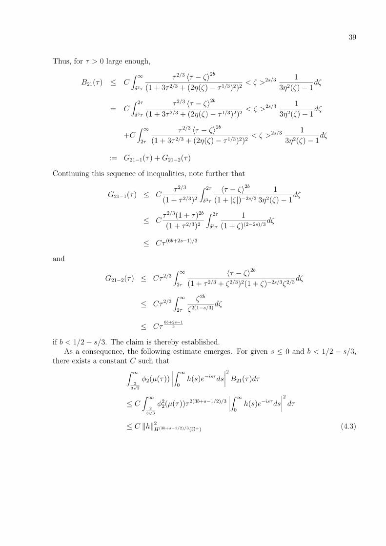
if b < 1/2− s/3. The claim is thereby established.As a consequence, the following estimate emerges. For given s ≤ 0 and b < 1/2 − s/3,

there exists a constant C such that∫ ∞

2

3√

3

φ2(µ(τ))∣∣∣∣∫ ∞

0h(s)e−isτds

∣∣∣∣2B21(τ)dτ

≤ C∫ ∞

2

3√

3

φ22(µ(τ))τ 2(3b+s−1/2)/3

∣∣∣∣∫ ∞

0h(s)e−isτds

∣∣∣∣2 dτ≤ C ‖h‖2

H(3b+s−1/2)/3(<+) (4.3)

40

for any h ∈ H(3b+s−1/2)/3(<+). The proof of Proposition 5.1 is complete. 2

Next, attention is given to the term∫ ∞

−∞

∫ ∞

−∞

⟨i(τ − (ξ3 − ρξ)) + ξ2

⟩2b< ξ >2s

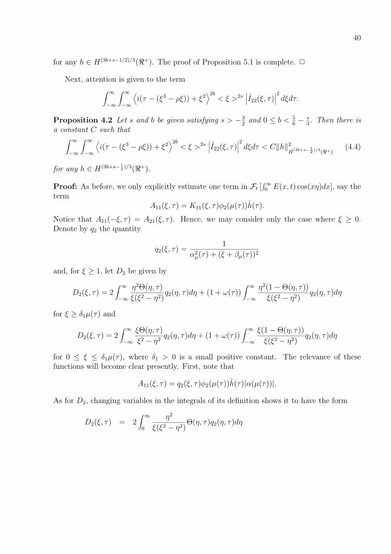
∣∣∣I22(ξ, τ)∣∣∣2 dξdτ.Proposition 4.2 Let s and b be given satisfying s > −3

2and 0 ≤ b < 5

6− s

3. Then there is

a constant C such that∫ ∞

−∞

∫ ∞

−∞

⟨i(τ − (ξ3 − ρξ)) + ξ2

⟩2b< ξ >2s

∣∣∣I22(ξ, τ)∣∣∣2 dξdτ < C‖h‖2

H(3b+s− 12 )/3(<+)

(4.4)

for any h ∈ H(3b+s− 12)/3(<+).

Proof: As before, we only explicitly estimate one term in Ft [∫∞0 E(x, t) cos(xη)dx], say the

termA11(ξ, τ) = K11(ξ, τ)φ2(µ(τ))h(τ).

Notice that A11(−ξ, τ) = A21(ξ, τ). Hence, we may consider only the case where ξ ≥ 0.Denote by q2 the quantity

q2(ξ, τ) =1

α2µ(τ) + (ξ + βµ(τ))2

and, for ξ ≥ 1, let D2 be given by

D2(ξ, τ) = 2∫ ∞

−∞

η2Θ(η, τ)

ξ(ξ2 − η2)q2(η, τ)dη + (1 + ω(τ))

∫ ∞

−∞

η2(1−Θ(η, τ))

ξ(ξ2 − η2)q2(η, τ)dη

for ξ ≥ δ1µ(τ) and

D2(ξ, τ) = 2∫ ∞

−∞

ξΘ(η, τ)

ξ2 − η2q2(η, τ)dη + (1 + ω(τ))

∫ ∞

−∞

ξ(1−Θ(η, τ))

ξ(ξ2 − η2)q2(η, τ)dη

for 0 ≤ ξ ≤ δ1µ(τ), where δ1 > 0 is a small positive constant. The relevance of thesefunctions will become clear presently. First, note that

A11(ξ, τ) = q2(ξ, τ)φ2(µ(τ))h(τ)|α(µ(τ))|.

As for D2, changing variables in the integrals of its definition shows it to have the form

D2(ξ, τ) = 2∫ ∞

0

η2

ξ(ξ2 − η2)Θ(η, τ)q2(η, τ)dη

41

+(1 + ω(τ))∫ ∞

0

η2

ξ(ξ2 − η2)(1−Θ(η, τ))q2(η, τ)dη

=2

µ2(τ)

∫ a0

0

η2

y(y2 − η2)Θ(µ(τ)η, τ)p2(η, τ)dη

+1 + ω(τ)

µ2(τ)

∫ ∞

a1

η2

y(y2 − η2)(1−Θ(µ(τ)η, τ))p2(η, τ)dη

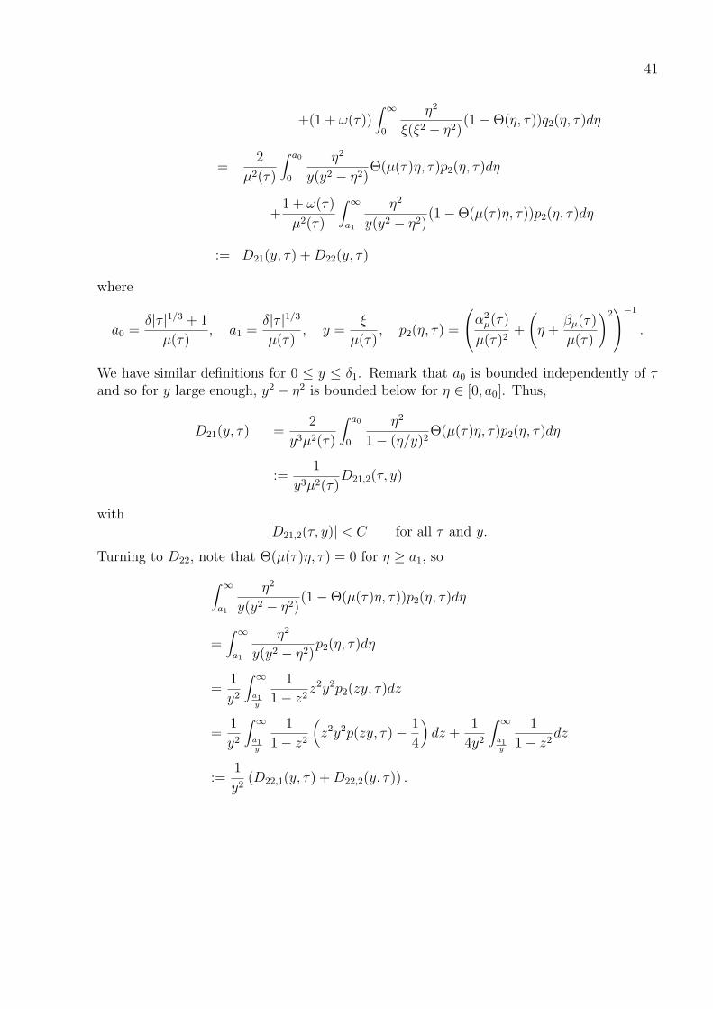
:= D21(y, τ) +D22(y, τ)

where

a0 =δ|τ |1/3 + 1

µ(τ), a1 =

δ|τ |1/3

µ(τ), y =

ξ

µ(τ), p2(η, τ) =

α2µ(τ)

µ(τ)2+

(η +

βµ(τ)

µ(τ)

)2−1

.

We have similar definitions for 0 ≤ y ≤ δ1. Remark that a0 is bounded independently of τand so for y large enough, y2 − η2 is bounded below for η ∈ [0, a0]. Thus,

D21(y, τ) =2

y3µ2(τ)

∫ a0

0

η2

1− (η/y)2Θ(µ(τ)η, τ)p2(η, τ)dη

:=1

y3µ2(τ)D21,2(τ, y)

with|D21,2(τ, y)| < C for all τ and y.

Turning to D22, note that Θ(µ(τ)η, τ) = 0 for η ≥ a1, so

∫ ∞

a1

η2

y(y2 − η2)(1−Θ(µ(τ)η, τ))p2(η, τ)dη

=∫ ∞

a1

η2

y(y2 − η2)p2(η, τ)dη

=1

y2

∫ ∞

a1y

1

1− z2z2y2p2(zy, τ)dz

=1

y2

∫ ∞

a1y

1

1− z2

(z2y2p(zy, τ)− 1

4

)dz +

1

4y2

∫ ∞

a1y

1

1− z2dz

:=1

y2(D22,1(y, τ) +D22,2(y, τ)) .

42

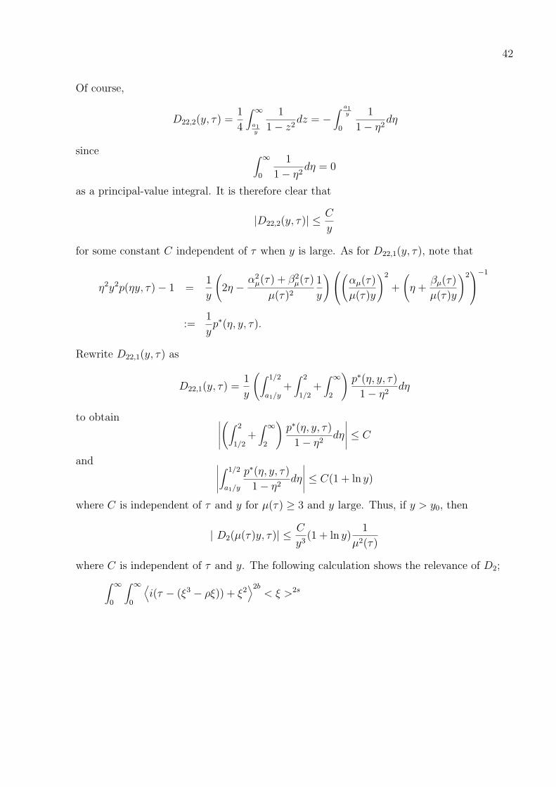
Of course,

D22,2(y, τ) =1

4

∫ ∞

a1y

1

1− z2dz = −

∫ a1y

0

1

1− η2dη

since ∫ ∞

0

1

1− η2dη = 0

as a principal-value integral. It is therefore clear that

|D22,2(y, τ)| ≤C

y

for some constant C independent of τ when y is large. As for D22,1(y, τ), note that

η2y2p(ηy, τ)− 1 =1

y

(2η −

α2µ(τ) + β2

µ(τ)

µ(τ)2

1

y

)(αµ(τ)

µ(τ)y

)2

+

(η +

βµ(τ)

µ(τ)y

)2−1

:=1

yp∗(η, y, τ).

Rewrite D22,1(y, τ) as

D22,1(y, τ) =1

y

(∫ 1/2

a1/y+∫ 2

1/2+∫ ∞

2

)p∗(η, y, τ)

1− η2dη

to obtain ∣∣∣∣∣(∫ 2

1/2+∫ ∞

2

)p∗(η, y, τ)

1− η2dη

∣∣∣∣∣ ≤ C

and ∣∣∣∣∣∫ 1/2

a1/y

p∗(η, y, τ)

1− η2dη

∣∣∣∣∣ ≤ C(1 + ln y)

where C is independent of τ and y for µ(τ) ≥ 3 and y large. Thus, if y > y0, then

| D2(µ(τ)y, τ)| ≤ C

y3(1 + ln y)

1

µ2(τ)

where C is independent of τ and y. The following calculation shows the relevance of D2;∫ ∞

0

∫ ∞

0

⟨i(τ − (ξ3 − ρξ)) + ξ2

⟩2b< ξ >2s

43

×∣∣∣∣∣∫ ∞

−∞

1

ξ − ηA11(η, τ)

(2Θ(η, τ) + (1−Θ(η, τ))(1 + ω(τ))

)dη

∣∣∣∣∣2

dξdτ

=∫ ∞

0

1

π2φ2

2(µ(τ))|h|2(τ)α2µ(τ)

∫ ∞

0

⟨i(τ − (ξ3 − ρξ)) + ξ2

⟩2b< ξ >2s

×∣∣∣∣∣∫ ∞

−∞

1

ξ − ηq2(η, τ)

(2Θ(η, τ) + (1−Θ(η, τ))(1 + ω(τ))

)dη

∣∣∣∣∣2

dξdτ

=∫ ∞

0

1

π2φ2

2(µ(τ))|h|2(τ)α2µ(τ)

∫ ∞

0

⟨i(τ − (ξ3 − ρξ)) + ξ2

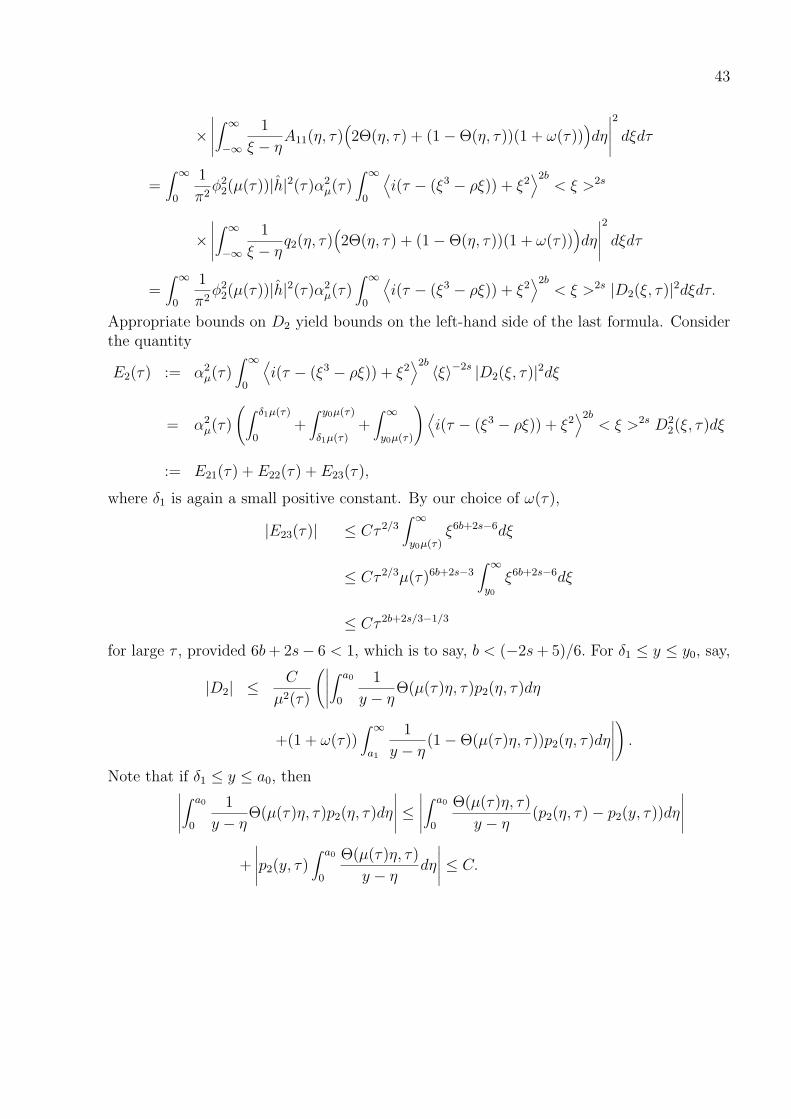
⟩2b< ξ >2s |D2(ξ, τ)|2dξdτ.

Appropriate bounds on D2 yield bounds on the left-hand side of the last formula. Considerthe quantity

E2(τ) := α2µ(τ)

∫ ∞

0

⟨i(τ − (ξ3 − ρξ)) + ξ2

⟩2b〈ξ〉−2s |D2(ξ, τ)|2dξ

= α2µ(τ)

(∫ δ1µ(τ)

0+∫ y0µ(τ)

δ1µ(τ)+∫ ∞

y0µ(τ)

)⟨i(τ − (ξ3 − ρξ)) + ξ2

⟩2b< ξ >2s D2

2(ξ, τ)dξ

:= E21(τ) + E22(τ) + E23(τ),

where δ1 is again a small positive constant. By our choice of ω(τ),

|E23(τ)| ≤ Cτ 2/3∫ ∞

y0µ(τ)ξ6b+2s−6dξ

≤ Cτ 2/3µ(τ)6b+2s−3∫ ∞

y0

ξ6b+2s−6dξ

≤ Cτ 2b+2s/3−1/3

for large τ , provided 6b+ 2s− 6 < 1, which is to say, b < (−2s+ 5)/6. For δ1 ≤ y ≤ y0, say,

|D2| ≤ C

µ2(τ)

(∣∣∣∣∣∫ a0

0

1

y − ηΘ(µ(τ)η, τ)p2(η, τ)dη

+(1 + ω(τ))∫ ∞

a1

1

y − η(1−Θ(µ(τ)η, τ))p2(η, τ)dη

∣∣∣∣∣).

Note that if δ1 ≤ y ≤ a0, then∣∣∣∣∣∫ a0

0

1

y − ηΘ(µ(τ)η, τ)p2(η, τ)dη

∣∣∣∣∣ ≤∣∣∣∣∣∫ a0

0

Θ(µ(τ)η, τ)

y − η(p2(η, τ)− p2(y, τ))dη

∣∣∣∣∣+

∣∣∣∣∣p2(y, τ)∫ a0

0

Θ(µ(τ)η, τ)

y − ηdη

∣∣∣∣∣ ≤ C.

44

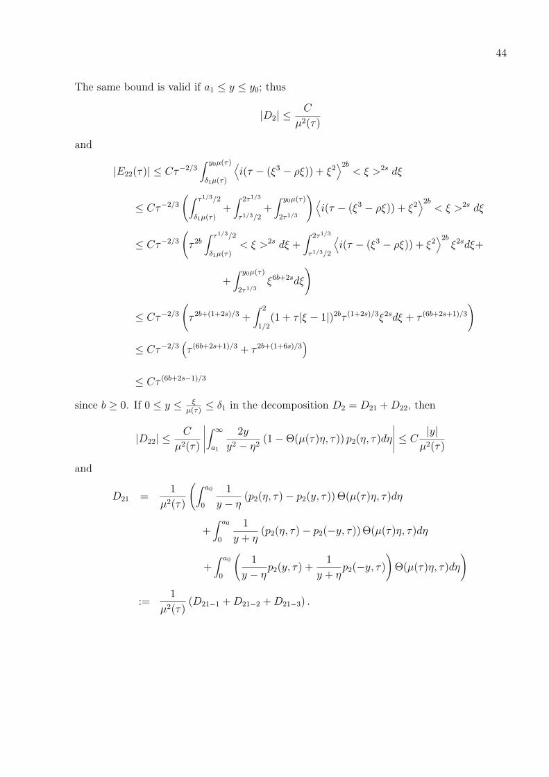
The same bound is valid if a1 ≤ y ≤ y0; thus

|D2| ≤C

µ2(τ)

and

|E22(τ)| ≤ Cτ−2/3∫ y0µ(τ)

δ1µ(τ)

⟨i(τ − (ξ3 − ρξ)) + ξ2

⟩2b< ξ >2s dξ

≤ Cτ−2/3

(∫ τ1/3/2

δ1µ(τ)+∫ 2τ1/3

τ1/3/2+∫ y0µ(τ)

2τ1/3

)⟨i(τ − (ξ3 − ρξ)) + ξ2

⟩2b< ξ >2s dξ

≤ Cτ−2/3

(τ 2b

∫ τ1/3/2

δ1µ(τ)< ξ >2s dξ +

∫ 2τ1/3

τ1/3/2

⟨i(τ − (ξ3 − ρξ)) + ξ2

⟩2bξ2sdξ+

+∫ y0µ(τ)

2τ1/3ξ6b+2sdξ

)

≤ Cτ−2/3

(τ 2b+(1+2s)/3 +

∫ 2

1/2(1 + τ |ξ − 1|)2bτ (1+2s)/3ξ2sdξ + τ (6b+2s+1)/3

)

≤ Cτ−2/3(τ (6b+2s+1)/3 + τ 2b+(1+6s)/3

)≤ Cτ (6b+2s−1)/3

since b ≥ 0. If 0 ≤ y ≤ ξµ(τ)

≤ δ1 in the decomposition D2 = D21 +D22, then

|D22| ≤C

µ2(τ)

∣∣∣∣∣∫ ∞

a1

2y

y2 − η2(1−Θ(µ(τ)η, τ)) p2(η, τ)dη

∣∣∣∣∣ ≤ C|y|µ2(τ)

and

D21 =1

µ2(τ)

(∫ a0

0

1

y − η(p2(η, τ)− p2(y, τ)) Θ(µ(τ)η, τ)dη

+∫ a0

0

1

y + η(p2(η, τ)− p2(−y, τ)) Θ(µ(τ)η, τ)dη

+∫ a0

0

(1

y − ηp2(y, τ) +

1

y + ηp2(−y, τ)

)Θ(µ(τ)η, τ)dη

)

:=1

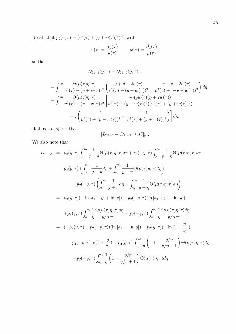
µ2(τ)(D21−1 +D21−2 +D21−3) .

45

Recall that p2(η, τ) = (v2(τ) + (η + w(τ))2)−1 with

v(τ) =αµ(τ)

µ(τ), w(τ) =

βµ(τ)

µ(τ),

so that

D21−1(y, τ) +D21−2(y, τ) =

=∫ a0

0

Θ(µ(τ)η, τ)

v2(τ) + (η + w(τ))2

(y + η + 2w(τ)

v2(τ) + (y + w(τ))2− η − y + 2w(τ)

v2(τ) + (−y + w(τ))2

)dη

=∫ a0

0

Θ(µ(τ)η, τ)

v2(τ) + (η − w(τ))2

[−4yw(τ)(η + 2w(τ))

v2(τ) + (y − w(τ))2)(v2(τ) + (y + w(τ))2)

+ y

(1

v2(τ) + (y − w(τ))2+

1

v2(τ) + (y + w(τ))2

)]dη.

It thus transpires that|D21−1 +D21−2| ≤ C|y|.

We also note that

D21−3 = p2(y, τ)∫ a0

0

1

y − ηΘ(µ(τ)η, τ)dη + p2(−y, τ)

∫ a0

0

1

y + ηΘ(µ(τ)η, τ)dη

= p2(y, τ)

(∫ a1

0

1

y − ηdη +

∫ a0

a1

1

y − ηΘ(µ(τ)η, τ)dη

)

+p2(−y, τ)(∫ a1

0

1

y + ηdη +

∫ a0

a1

1

y + ηΘ(µ(τ)η, τ)dη

)

= p2(y, τ)(− ln |a1 − y|+ ln |y|) + p2(−y, τ)(ln |a1 + y| − ln |y|)

+p2(y, τ)∫ a0

a1

1

η

Θ(µ(τ)η, τ)dη

y/η − 1+ p2(−y, τ)

∫ a0

a1

1

η

Θ(µ(τ)η, τ)dη

y/η + 1

= (−p2(y, τ) + p2(−y, τ))(ln |a1| − ln |y|) + p2(y, τ)(− ln |1− y

a1

|)

+p2(−y, τ) ln(1 +y

a1

) + p2(y, τ)∫ a0

a1

1

η

(−1 +

y/η

y/η − 1

)Θ(µ(τ)η, τ)dη

+p2(−y, τ)∫ a0

a1

1

η

(1− y/η

y/η + 1

)Θ(µ(τ)η, τ)dη

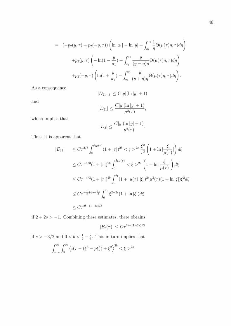
46

= (−p2(y, τ) + p2(−y, τ))(

ln |a1| − ln |y|+∫ a0

a1

1

ηΘ(µ(τ)η, τ)dη

)

+p2(y, τ)

(− ln(1− y

a1

) +∫ a0

a1

y

(y − η)ηΘ(µ(τ)η, τ)dη

)

+p2(−y, τ)(

ln(1 +y

a1

)−∫ a0

a1

y

(y + η)ηΘ(µ(τ)η, τ)dη

).

As a consequence,|D21−3| ≤ C|y|(ln |y|+ 1)

and

|D21| ≤C|y|(ln |y|+ 1)

µ2(τ),

which implies that

|D2| ≤C|y|(ln |y|+ 1)

µ2(τ).

Thus, it is apparent that

|E21| ≤ Cτ 2/3∫ δ1µ(τ)

0(1 + |τ |)2b < ξ >2s ξ

2

τ 2

(1 + ln | ξ

µ(τ)|)dξ

≤ Cτ−4/3(1 + |τ |)2b∫ δ1µ(τ)

0< ξ >2s

(1 + ln | ξ

µ(τ)|)dξ

≤ Cτ−4/3(1 + |τ |)2b∫ δ1

0(1 + |µ(τ)||ξ|)2sµ3(τ)(1 + ln |ξ|)ξ2dξ

≤ Cτ−13+2b+ 2s

3

∫ δ1

0ξ2+2s(1 + ln |ξ|)dξ

≤ Cτ 2b−(1−2s)/3

if 2 + 2s > −1. Combining these estimates, there obtains

|E2(τ)| ≤ Cτ 2b−(1−2s)/3

if s > −3/2 and 0 < b < 12− s

3. This in turn implies that∫ ∞

−∞

∫ ∞

0

⟨i(τ − (ξ3 − ρξ)) + ξ2

⟩2b< ξ >2s

47

∣∣∣∣∣∫ ∞

−∞

1

ξ − ηA21(η, τ)×

(2Θ(η, τ) + (1−Θ(η, τ))(1 + ω(τ))

)dη

∣∣∣∣∣2

dξdτ

≤ C∫ ∞

0τ 2b−(1−2s)/3

∣∣∣∣∫ ∞

0h(s)e−isτds

∣∣∣∣2 dτ≤ C‖h‖2

Hb+ s3−

16.

Similar estimates for other terms yield, in sum,∫ ∞

−∞

∫ ∞

−∞

⟨i(τ − (ξ3 − ρξ)) + ξ2

⟩2b< ξ >2s

∣∣∣I22(ξ, τ)∣∣∣2 dξdτ ≤ C‖h‖2

Hb+ s3−

16

if −32< s ≤ 0 and 0 ≤ b < 1

2− s

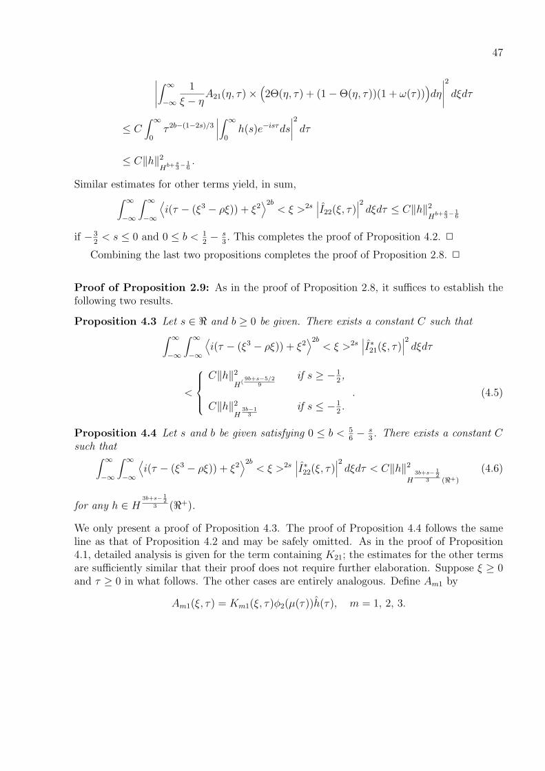
3. This completes the proof of Proposition 4.2. 2

Combining the last two propositions completes the proof of Proposition 2.8. 2

Proof of Proposition 2.9: As in the proof of Proposition 2.8, it suffices to establish thefollowing two results.

Proposition 4.3 Let s ∈ < and b ≥ 0 be given. There exists a constant C such that∫ ∞

−∞

∫ ∞

−∞

⟨i(τ − (ξ3 − ρξ)) + ξ2

⟩2b< ξ >2s

∣∣∣I∗21(ξ, τ)∣∣∣2 dξdτ

<

C‖h‖2

H(9b+s−5/2

9

if s ≥ −12,

C‖h‖2

H3b−1

3if s ≤ −1

2.. (4.5)

Proposition 4.4 Let s and b be given satisfying 0 ≤ b < 56− s

3. There exists a constant C

such that∫ ∞

−∞

∫ ∞

−∞

⟨i(τ − (ξ3 − ρξ)) + ξ2

⟩2b< ξ >2s

∣∣∣I∗22(ξ, τ)∣∣∣2 dξdτ < C‖h‖2

H3b+s− 1

23 (<+)

(4.6)

for any h ∈ H3b+s− 1

23 (<+).

We only present a proof of Proposition 4.3. The proof of Proposition 4.4 follows the sameline as that of Proposition 4.2 and may be safely omitted. As in the proof of Proposition4.1, detailed analysis is given for the term containing K21; the estimates for the other termsare sufficiently similar that their proof does not require further elaboration. Suppose ξ ≥ 0and τ ≥ 0 in what follows. The other cases are entirely analogous. Define Am1 by

Am1(ξ, τ) = Km1(ξ, τ)φ2(µ(τ))h(τ), m = 1, 2, 3.

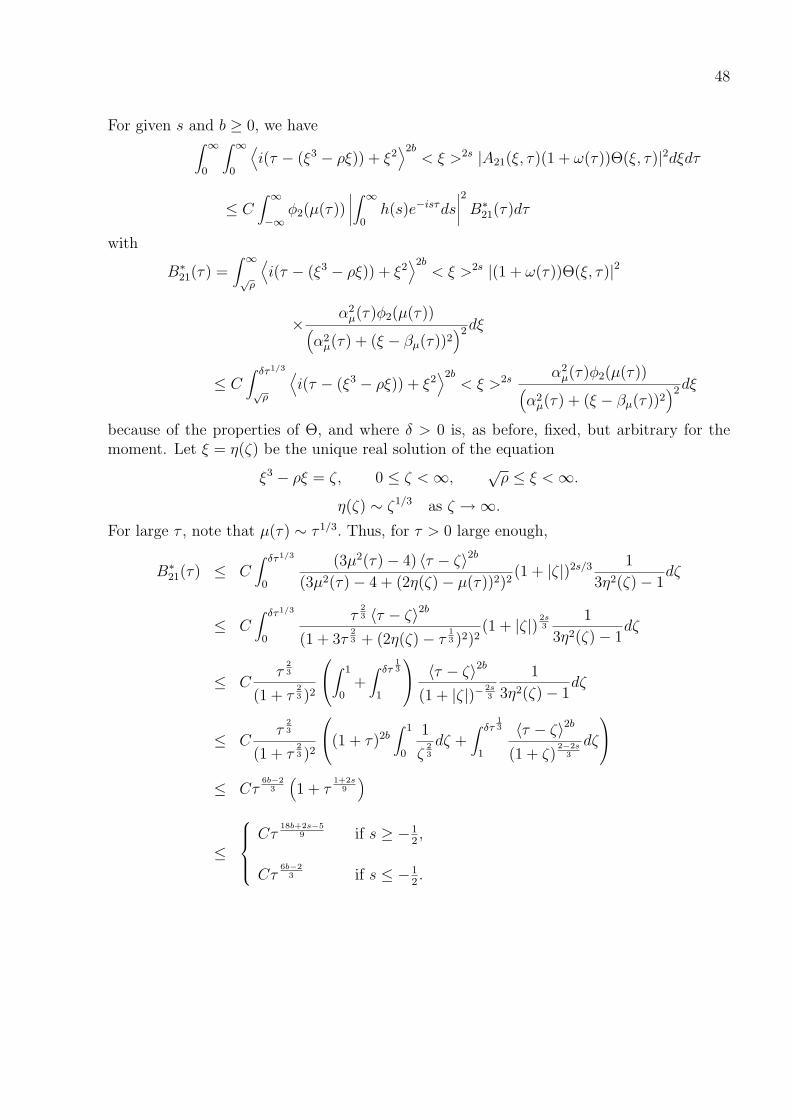
48

For given s and b ≥ 0, we have∫ ∞

0

∫ ∞

0

⟨i(τ − (ξ3 − ρξ)) + ξ2

⟩2b< ξ >2s |A21(ξ, τ)(1 + ω(τ))Θ(ξ, τ)|2dξdτ

≤ C∫ ∞

−∞φ2(µ(τ))

∣∣∣∣∫ ∞

0h(s)e−isτds

∣∣∣∣2B∗21(τ)dτ

with

B∗21(τ) =

∫ ∞

√ρ

⟨i(τ − (ξ3 − ρξ)) + ξ2

⟩2b< ξ >2s |(1 + ω(τ))Θ(ξ, τ)|2

×α2

µ(τ)φ2(µ(τ))(α2

µ(τ) + (ξ − βµ(τ))2)2dξ

≤ C∫ δτ1/3

√ρ

⟨i(τ − (ξ3 − ρξ)) + ξ2

⟩2b< ξ >2s α2

µ(τ)φ2(µ(τ))(α2

µ(τ) + (ξ − βµ(τ))2)2dξ

because of the properties of Θ, and where δ > 0 is, as before, fixed, but arbitrary for themoment. Let ξ = η(ζ) be the unique real solution of the equation

ξ3 − ρξ = ζ, 0 ≤ ζ <∞,√ρ ≤ ξ <∞.

η(ζ) ∼ ζ1/3 as ζ →∞.

For large τ , note that µ(τ) ∼ τ 1/3. Thus, for τ > 0 large enough,

B∗21(τ) ≤ C

∫ δτ1/3

0

(3µ2(τ)− 4) 〈τ − ζ〉2b

(3µ2(τ)− 4 + (2η(ζ)− µ(τ))2)2(1 + |ζ|)2s/3 1

3η2(ζ)− 1dζ

≤ C∫ δτ1/3

0

τ23 〈τ − ζ〉2b

(1 + 3τ23 + (2η(ζ)− τ

13 )2)2

(1 + |ζ|)2s3

1

3η2(ζ)− 1dζ

≤ Cτ

23

(1 + τ23 )2

∫ 1

0+∫ δτ

13

1

〈τ − ζ〉2b

(1 + |ζ|)− 2s3

1

3η2(ζ)− 1dζ

≤ Cτ

23

(1 + τ23 )2

(1 + τ)2b∫ 1

0

1

ζ23

dζ +∫ δτ

13

1

〈τ − ζ〉2b

(1 + ζ)2−2s

3

dζ

≤ Cτ

6b−23

(1 + τ

1+2s9

)

≤

Cτ

18b+2s−59 if s ≥ −1

2,

Cτ6b−2

3 if s ≤ −12.

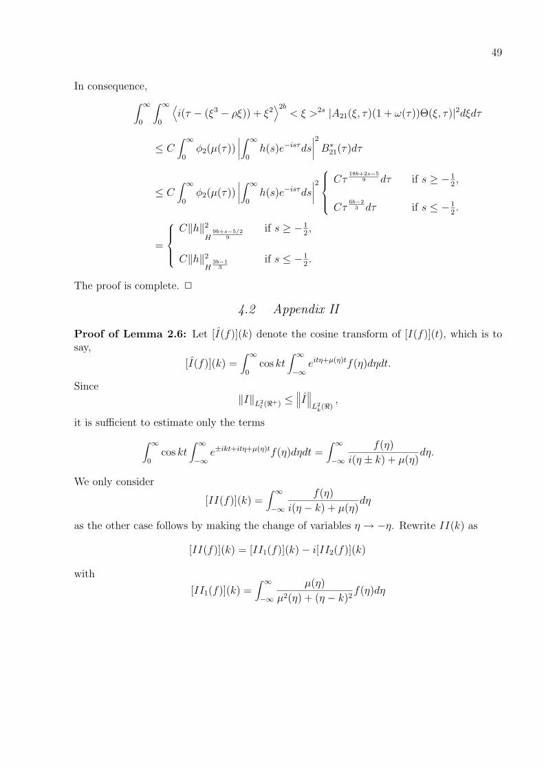
49

In consequence,∫ ∞

0

∫ ∞

0

⟨i(τ − (ξ3 − ρξ)) + ξ2

⟩2b< ξ >2s |A21(ξ, τ)(1 + ω(τ))Θ(ξ, τ)|2dξdτ

≤ C∫ ∞

0φ2(µ(τ))

∣∣∣∣∫ ∞

0h(s)e−isτds

∣∣∣∣2B∗21(τ)dτ

≤ C∫ ∞

0φ2(µ(τ))

∣∣∣∣∫ ∞

0h(s)e−isτds

∣∣∣∣2Cτ

18b+2s−59 dτ if s ≥ −1

2,

Cτ6b−2

3 dτ if s ≤ −12.

=

C‖h‖2

H9b+s−5/2

9

if s ≥ −12,

C‖h‖2

H3b−1

3if s ≤ −1

2.

The proof is complete. 2

4.2 Appendix II

Proof of Lemma 2.6: Let [I(f)](k) denote the cosine transform of [I(f)](t), which is tosay,

[I(f)](k) =∫ ∞

0cos kt

∫ ∞

−∞eitη+µ(η)tf(η)dηdt.

Since‖I‖L2

t (<+) ≤∥∥∥I∥∥∥

L2k(<),

it is sufficient to estimate only the terms∫ ∞

0cos kt

∫ ∞

−∞e±ikt+itη+µ(η)tf(η)dηdt =

∫ ∞

−∞

f(η)

i(η ± k) + µ(η)dη.

We only consider

[II(f)](k) =∫ ∞

−∞

f(η)

i(η − k) + µ(η)dη

as the other case follows by making the change of variables η → −η. Rewrite II(k) as

[II(f)](k) = [II1(f)](k)− i[II2(f)](k)

with

[II1(f)](k) =∫ ∞

−∞

µ(η)

µ2(η) + (η − k)2f(η)dη

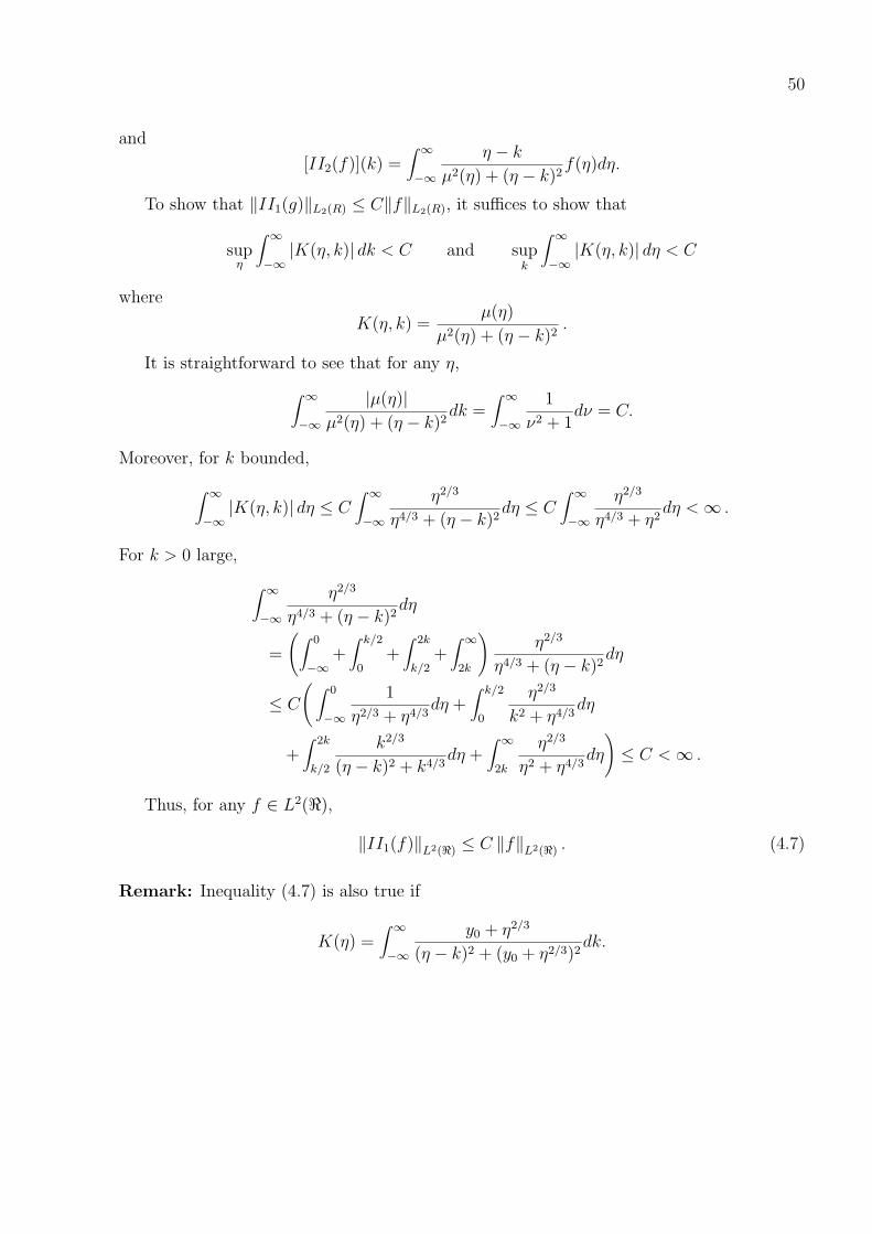
50

and

[II2(f)](k) =∫ ∞

−∞

η − k

µ2(η) + (η − k)2f(η)dη.

To show that ‖II1(g)‖L2(R) ≤ C‖f‖L2(R), it suffices to show that

supη

∫ ∞

−∞|K(η, k)| dk < C and sup

k

∫ ∞

−∞|K(η, k)| dη < C

where

K(η, k) =µ(η)

µ2(η) + (η − k)2.

It is straightforward to see that for any η,∫ ∞

−∞

|µ(η)|µ2(η) + (η − k)2

dk =∫ ∞

−∞

1

ν2 + 1dν = C.

Moreover, for k bounded,

∫ ∞

−∞|K(η, k)| dη ≤ C

∫ ∞

−∞

η2/3

η4/3 + (η − k)2dη ≤ C

∫ ∞

−∞

η2/3

η4/3 + η2dη <∞ .

For k > 0 large,

∫ ∞

−∞

η2/3

η4/3 + (η − k)2dη

=

(∫ 0

−∞+∫ k/2

0+∫ 2k

k/2+∫ ∞

2k

)η2/3

η4/3 + (η − k)2dη

≤ C

(∫ 0

−∞

1

η2/3 + η4/3dη +

∫ k/2

0

η2/3

k2 + η4/3dη

+∫ 2k

k/2

k2/3

(η − k)2 + k4/3dη +

∫ ∞

2k

η2/3

η2 + η4/3dη

)≤ C <∞ .

Thus, for any f ∈ L2(<),

‖II1(f)‖L2(<) ≤ C ‖f‖L2(<) . (4.7)

Remark: Inequality (4.7) is also true if

K(η) =∫ ∞

−∞

y0 + η2/3

(η − k)2 + (y0 + η2/3)2dk.

51

To study II2, let 0 < a ≤ ∞ be given and consider the function

Φa(z) =∫ a

−a

f(t)

i(t− z)− µ(t)dt.

It is analytic in the region Im z > 0 since the zeros of i(t − z) + µ(t) are z = t + iµ(t). Inaddition, if f(t) is compactly supported, then

Φa(z) ∼ O

(1

|z|

)as |z| → ∞

and the implied constant is independent of a.For given r > 0 and y0 > 0, let Cr denote the closed curve in the z−plane which is taken

along the line from −r + iy0 to r + iy0 with y0 > 0 and then around the semicircle above itof radius r centered at iy0 in the counterclockwise direction. By Cauchy’s theorem,∫

Cr

Φa(z)2dz = 0

which, upon taking the limit as r →∞, yields∫ ∞

−∞Φ1(x+ iy0))

2dx = 0.

SinceΦa(x+ iy0) = Ua(x+ iy0) + iVa(x+ iy0)

with

Ua(x+ iy0) =∫ a

−a

y0 − µ(t)

(t− x)2 + (y0 − µ(t))2f(t)dt

and

Va(x+ iy0) = −∫ a

−a

t− x

(t− x)2 + (y0 − µ(t))2f(t)dt,

it follows that ∫ ∞

−∞U2

a (x+ iy0)dx =∫ ∞

−∞V 2

a (x+ iy0)dx

and hence by Fubini’s theorem,

∫ ∞

−∞V 2

a (x+ iy0)dx ≤∫ ∞

−∞

(∫ ∞

−∞

y0 − µ(t)

(t− x)2 + (y0 − µ(t))2|f(t)|dt

)2

dx

≤ C ‖f‖2L2(<) .

52

Taking y0 → 0 and applying Fatou’s Lemma leads to the conclusion

∫ ∞

−∞

(∫ a

−a

t− x

(t− x)2 + µ2(t)|f(t)|dt

)2

dx ≤ C ‖f‖2L2(<) .

Then, letting a→∞ and using Fatou’s Lemma again yields

∫ ∞

−∞

(∫ ∞

−∞

t− x

(t− x)2 + µ2(t)|f(t)|dt

)2

dx ≤ C ‖f‖2L2(<)

for all compactly supported f . The proof is complete. 2

References

[1] D. Bekiranov, The initial-value problem for the generalized Burgers’ equation, Diff.Intgeral Eq. 9 (1996), 1253–1265.

[2] B. Boczar-Karakiewicz and J. L. Bona, Wave dominated shelves: a model of sand ridgeformation by progressive infragravity waves. In Shelf Sands and Sandstones (ed. R.J.Knight and J. R. McLean) Canadian Society of Petroleum Geologists memoir 11 (1986),163 – 179.

[3] J. L. Bona and P. J. Bryant, A mathematical model for long waves generated by wavemakers in nonlinear dispersive systems, Proc. Cambridge Philos. Soc. 73 (1973), 391 –405.

[4] J. L. Bona and L. Luo, Generalized Korteweg-de Vries equation in a quarter plane,Contemp. Math. 221 (1999), 59 – 125.

[5] J. L. Bona, W. G. Pritchard and L. R. Scott, An evaluation of a model equation forwater waves, Philos. Trans. Royal Soc. London Series A 302 (1981), 457 – 510.

[6] J. L. Bona and L. R. Scott, Solutions of the Korteweg-de Vries equation in fractionalorder Sobolev spaces, Duke Math. J. 43 (1976), 87 – 99.

[7] J. L. Bona and R. Smith, The initial-value problem for the Korteweg-de Vries equation,Philos. Trans. Royal Soc. London Series A 278 (1975), 555 – 601.

[8] J. L. Bona, S. Sun and B.-Y. Zhang, A nonhomogeneous boundary-value problem for theKorteweg-de Vries equation in a quarter plane, Trans. American Math. Soc. 354 (2001),427 – 490.

53

[9] J. L. Bona, S. Sun and B.-Y. Zhang, Forced oscillations of a damped KdV equation ina quarter plane, Commun. Contemp. Math. 5 (2003), 369–400.

[10] J. L. Bona, S. Sun and B.-Y. Zhang, A nonhomogeneous boundary value problem for theKdV equation posed on a finite domain, Commun. Partial Differential Eq. 28 (2003),1391–1436.

[11] J. L. Bona, S. Sun and B.-Y. Zhang, Conditional and unconditional well-posedness ofnonlinear evolution equations, Adv. Differential Eq. 9 (2004), 241 – 265.

[12] J. L. Bona, S. Sun and B.-Y. Zhang, Boundary smoothing properties of the Korteweg-deVries equation in a quarter plane and applications, Dynamics Partial Differential Eq.3 (2006), 1 – 70.

[13] J. L. Bona and R. Winther, The Korteweg-de Vries equation, posed in a quarter plane,SIAM J. Math. Anal. 14 (1983), 1056 – 1106.

[14] J. L. Bona and R. Winther, Korteweg-de Vries equation in a quarter plane, continuousdependence results, Differential Integral Eq. 2 (1989), 228 – 250.

[15] J. Bourgain, Fourier transform restriction phenomena for certain lattice subsets andapplications to non-linear evolution equations, part II: the KdV equation, Geom. &Funct. Anal. 3 (1993), 209 – 262.

[16] J. Bourgain, Periodic Korteweg-de Vries equation with measures as initial data, SelectaMath. (N.S.) 3 (1997), 115–159.

[17] A. Cohen, Solutions of the Korteweg-de Vries equation from irregular data, Duke Math.J. 45 (1978), 149 – 181.

[18] A. Cohen, Existence and regularity for solutions of the Korteweg-de Vries equation,Arch. Rat. Mech. Anal. 71 (1979), 143 – 175.

[19] M. Christ, J. Colliander and T. Tao, Asymptotics, frequency modulation, and lowregularity ill-posedness for canonical defocusing equations, Amer. J. Math.125 (2003),1235–1293.

[20] J. E. Colliander and C. E. Kenig, The generalized Korteweg-de Vries equation on thehalf line, Comm. Partial Differential Eq. 27 (2002), 2187–2266.

[21] J. E. Colliander, M. Keel, G. Staffilani, H. Takaoka and T. Tao, Sharp global well-posedness for KdV and modified KdV on R and T , J. American Math. Soc. 16 (2003),705–749

54

[22] P. Constantin and J.-C. Saut, Local smoothing properties of dispersive equations, J.American Math. Soc. 1 (1988), 413 – 446.

[23] W. Craig, T. Kappeler and W. A. Strauss, Gain of regularity for equations of theKorteweg-de Vries type, Ann. Inst. Henri Poincare 9 (1992), 147 – 186.

[24] D. B. Dix, The dissipation of nonlinear dispersive waves: the case of asymptoticallyweak nonlinearity, Comm. Partial Differential Eq. 17 (1992), 1665-1693.

[25] D. B. Dix, Nonuniqueness and uniqueness in the initial-value problem for Burgers’equation, SIAM J. Math. Anal. 27 (1996), 708–724.

[26] A. V. Faminskii, The Cauchy problem and the mixed problem in the half strip forequations of Korteweg- de Vries type, (Russian) Dinamika Sploshn. Sredy 162 (1983),152 – 158.

[27] A. V. Faminskii, A mixed problem in a semistrip for the Korteweg-de Vries equationand its generalizations, (Russian) Dinamika Sploshn. Sredy 258 (1988), 54 – 94; Englishtransl.. in Trans. Moscow Math. Soc. 51 (1989), 53 – 91.

[28] A. V. Faminskii, Mixed problems for the Korteweg-de Vries equation, Sbornik: Mathe-matics 190 (1999), 903–935.

[29] A. V. Faminskii, An initial boundary-value problem in a half-strip for the Korteweg-deVries equation in fractional-order Sobolev spaces, Comm. Partial Differential Eq.29(2004), 1653–1695,

[30] A. S. Fokas and A. R. Its, Soliton generation for initial-boundary value problems, Phys.Rev. Lett. 68 (1992), 3117 – 3120.

[31] A. S. Fokas and A. R. Its, An initial-boundary value problem for the Korteweg-de Vriesequation, In the proceedings of the conference: Solitons, nonlinear wave equations andcomputation (New Brunswick, NJ, 1992), Math. Comput. Simulation 37 (1994), 293 –321.

[32] A. S. Fokas and A. R. Its, Integrable equations on the half-infinite line. Solitons in scienceand engineering: theory and applications, Chaos Solitons Fractals 5 (1995), 2367 – 2376.

[33] A. S. Fokas and B. Pelloni, The solution of certain initial boundary-value problemsfor the linearized Korteweg-de Vries equation, Proc. Royal. Soc. London Series A454 (1998), 645 – 657.

[34] G. H. Hardy, J. E. Littlewood and G. Polya, Inequalities, Cambridge University Press:Cambridge (1934).

55

[35] J. Holmer, The initial-boundary value problem for the Korteweg-de Vries equation, toappear in Commun. Partial Differential Eq..

[36] R. S. Johnson, A nonlinear equation incorporating damping and dispersion, J. FluidMechanics 42 (1970), 49 – 60.

[37] T. Kappeler and P. Topalov, Well-posedness of KDV on H−1(T ), to appear in DukeMath. J.

[38] T. Kato, On the Korteweg-de Vries equation, Manuscripta Math. 29 (1979), 89 – 99.

[39] T. Kato, The Cauchy problem for the Korteweg-de Vries equation, Pitman ResearchNotes in Math. 53 (1979), 293 – 307.

[40] T. Kato, On the Cauchy problem for the (generalized) Korteweg-de Vries equations,Advances in Mathematics Supplementary Studies, Studies Appl. Math. 8 (1983), 93 –128.

[41] C. E. Kenig, G. Ponce and L. Vega, On the (generalized) Korteweg-de Vries equation,Duke Math. J. 59 (1989), 585 – 610.

[42] C. E. Kenig, G. Ponce and L. Vega, Well-posedness of the initial value problem for theKdV equation, J. American Math. Soc. 4 (1991), 323 – 347.

[43] C. E. Kenig, G. Ponce and L. Vega, Well-posedness and scattering results for the gen-eralized Korteweg-de Vries equations via the contraction principle, Comm. Pure Appl.Math. 46 (1993), 527 – 620.

[44] C. E. Kenig, G. Ponce and L. Vega, The Cauchy problem for the Korteweg-de Vriesequation in Sobolev spaces of negative indices, Duke Math. J. 71 (1993), 1 – 21.

[45] C. E. Kenig, G. Ponce and L. Vega, A bilinear estimate with applications to the KdVequation, J. American Math. Soc. 9 (1996), 573 – 603.

[46] C. E. Kenig, G. Ponce and L. Vega, On the ill-posedness of some canonical dispersiveequations, Duke Math. J. 106 (2001), 617-633.

[47] S. N. Kruzhkov and A. V. Faminskii, Generalized solutions of the Cauchy problemfor the Korteweg-de Vries equation, (Russian) Mat. Sb. (N.S.) 120 (1983), 396 – 425:English translation in Math USSSR Sbornik 48 (1984), 391 – 421.

[48] J.-L. Lions and E. Magenes, Non-homogeneous boundary value problems and applica-tions, Vol. 1, Springer-Verlag: Heidelberg (1972).

56

[49] L. Molinet and F. Ribaud, On the low regularity of the Korteweg-de Vries-Burgersequation, International Math. Res. Notices 37 (2002), 1979-2005.

[50] D. L. Russell and B.-Y. Zhang, Smoothing properties of solutions of the Korteweg-de Vries equation on a periodic domain with point dissipation, J. Math. Anal. Appl.190 (1995), 449 – 488.

[51] J.-C. Saut and R. Temam, Remarks on the Korteweg-de Vries equation, Israel J. Math.24 (1976), 78 – 87.

[52] A. Sjoberg, On the Korteweg-de Vries equation: Existence and uniqueness, J. Math.Anal. Appl. 29 (1970), 569 – 579.

[53] E. M. Stein and G. Weiss, Introduction to Fourier Analysis on Euclidean Spaces, Prince-ton University Press: Princeton (1971).

[54] L. Tartar, Interpolation non lineaire et regularite, J. Funct. Anal. 9 (1972), 469 – 489.

[55] R. Temam, Sur un probleme non lineaire, J. Math. Pures Appl. 48 (1969), 159 – 172.

[56] B. A. Ton, Initial boundary value problems for the Korteweg-de Vries equation, J.Differential Eq. 25 (1977), 288–309.

[57] N. Tzvetkov, Remark on the local ill-posedness for the KdV equation, C. R. Acad. Sci.Paris Ser. I Math. 329 (1999), 1043–1047.

[58] B.-Y. Zhang, Analyticity of solutions for the generalized Korteweg-de Vries equationwith respect to their initial datum, SIAM J. Math. Anal. 26 (1995), 1488 – 1513.