Boundary conditions Inﬂow and outﬂowgtryggva/CFD-Course/2013-Lecture-22.pdf · Periodic...

Computational Fluid Dynamics

Solving the Navier-Stokes Equations-II!

Grétar Tryggvason!Spring 2013!

http://www.nd.edu/~gtryggva/CFD-Course/!Computational Fluid Dynamics

Boundary Conditions for Inflow and Outflow!Compact schemes!Conservation of energy!Higher order in time for ! the ψ-ω formulation!

Outline!


The Artificial Compressibility Method !(Chorin, 1967, JCP 2, 12-26)!

∂u∂t

= −A(u) + ν∇2u − ∇p

∂ p∂t

= −1c2 ∇ ⋅u

c is a numerical parameter, in effect an artificial velocity of sound. At steady state !

�

∇ ⋅u = 0


Boundary conditions!Inflow and outflow!


Boundary conditions!

Fully enclosed flow!!Driven cavity!

!Internal flow (inflow & outflow)!!External flow!

!Flow over bodies!


For fully enclosed domains, such as in the driven cavity problem, the application of the boundary conditions is relatively straight forward.!

For domains with inflows it is usually reasonable to specify the velocity profile at the inlet!

The major problem is how to handle outflow boundaries in such a way that the fluid leaves in a “physically plausible” way!


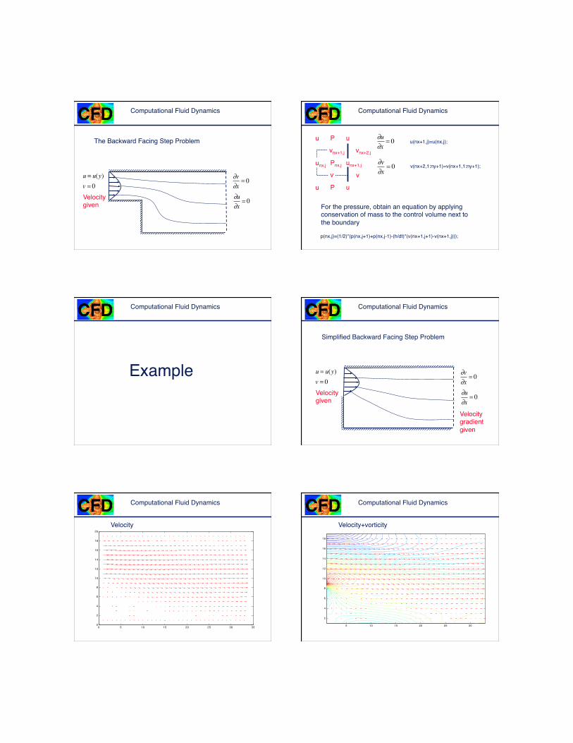
The Backward Facing Step Problem!

Velocity given!

�

u = u(y)v = 0

�

∂u∂x

= 0

�

∂v∂x

= 0


u!

vnx+1,j!

P!

unx,j! Pnx,j!

u! P!

v!

u!

unx+1,j!

u!

vnx+2,j!

v!v(nx+2,1:ny+1)=v(nx+1,1:ny+1);!

u(nx+1,j)=u(nx,j);!

p(nx,j)=(1/2)*(p(nx,j+1)+p(nx,j-1)-(h/dt)*(v(nx+1,j+1)-v(nx+1,j)));!!

�

∂u∂x

= 0

�

∂v∂x

= 0

For the pressure, obtain an equation by applying conservation of mass to the control volume next to the boundary!


Example!


Simplified Backward Facing Step Problem!

Velocity given!

�

u = u(y)v = 0

�

∂u∂x

= 0

Velocity gradient given!

�

∂v∂x

= 0


0 5 10 15 20 25 30 350

2

4

6

8

10

12

14

16

18

20

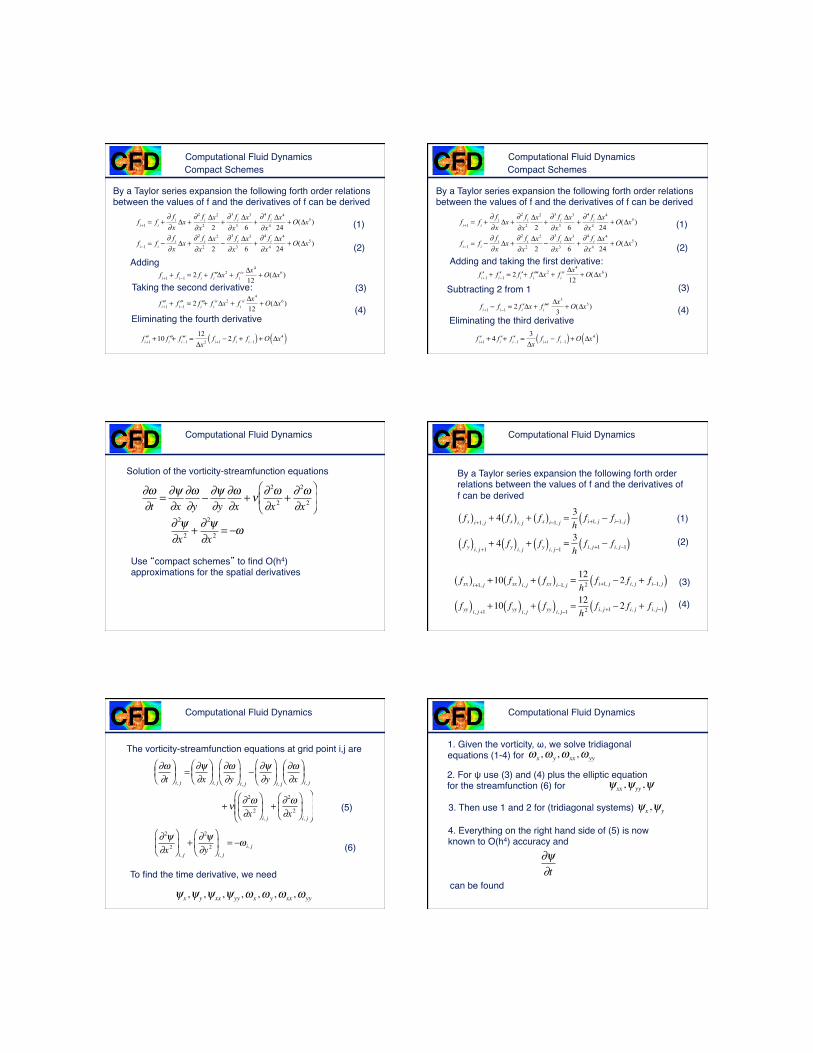
Velocity!


5 10 15 20 25 30

2

4

6

8

10

12

14

16

18

Velocity+vorticity!


05

1015

20

0

10

20

30

40-2.5

-2

-1.5

-1

-0.5

0

0.5

Pressure!

Inflow!


Periodic Boundary conditions!In many cases it is possible to use periodic boundary conditions, where what flows out through one boundary reappears flowing in through the opposite boundary. Such conditions are particularly suitable for theoretical studies of idealized flows. For such boundaries it is easiest to specify the pressure drop, but by adjusting the pressure gradient it is possible to specify the volume flux!


External flow!

Free outflow!

Free stream (uniform flow, for example)!

Boundary of computational domain!


Other ways to deal with free-stream boundaries!!Include potential flow perturbation!!Compute flow from vorticity distribution!!Map the boundary at infinity to a finite distance!

Fundamentally, the specification of the boundary conditions does not have a unique solution and is also faced by experimentalists. However, by taking the boundaries far away and checking the solution for the effect of moving the boundaries, good results can be obtained!


Compact schemes!


The standard way to obtain higher order approximations to derivatives is to include more points. This can lead to very wide stencils and near boundaries this requires a large number of “ghost” points outside the boundary. This can be overcome by “compact” schemes, where we derive expressions relating the derivatives at neighboring points to each other and the function values.!

Compact Schemes!


By a Taylor series expansion the following forth order relations between the values of f and the derivatives of f can be derived!

(1)!

(2)!

(3)!

(4)!

Adding!

fi+1 = fi +∂ fi

∂xΔx +

∂ 2 fi

∂x2

Δx2

2+∂ 3 fi

∂x3

Δx3

6+∂ 4 fi

∂x4

Δx4

24+ O(Δx5)

fi−1 = fi −∂ fi

∂xΔx +

∂ 2 fi

∂x2

Δx2

2−∂ 3 fi

∂x3

Δx3

6+∂ 4 fi

∂x4

Δx4

24+ O(Δx5)

′′fi+1 + ′′fi−1 = 2 ′′fi + fi

ivΔx2 + fivi Δx4

12+ O(Δx6 )

fi+1 + fi−1 = 2 fi + ′′fi Δx2 + fi

iv Δx4

12+ O(Δx6 )

Taking the second derivative:!

Eliminating the fourth derivative!

′′fi+1 +10 ′′fi + ′′fi−1 =

12Δx2 fi+1 − 2 fi + fi−1( ) + O Δx4( )

Compact Schemes!Computational Fluid Dynamics


(1)!

(2)!

(3)!

(4)!

fi+1 = fi +∂ fi

∂xΔx +

∂ 2 fi

∂x2

Δx2

2+∂ 3 fi

∂x3

Δx3

6+∂ 4 fi

∂x4

Δx4

24+ O(Δx5)

fi−1 = fi −∂ fi

∂xΔx +

∂ 2 fi

∂x2

Δx2

2−∂ 3 fi

∂x3

Δx3

6+∂ 4 fi

∂x4

Δx4

24+ O(Δx5)

′fi+1 + ′fi−1 = 2 ′fi + ′′′fi Δx2 + fi

iv Δx4

12+ O(Δx6 )

Adding and taking the first derivative:!

Subtracting 2 from 1!

′fi+1 + 4 ′fi + ′fi−1 =

3Δx

fi+1 − fi−1( ) + O Δx4( )

fi+1 − fi−1 = 2 ′fi Δx + ′′′fi

Δx3

3+ O(Δx5)

Eliminating the third derivative!

Compact Schemes!


�

∂ω∂t

= ∂ψ∂x

∂ω∂y

− ∂ψ∂y

∂ω∂x

+ ν ∂ 2ω∂x 2

+ ∂ 2ω∂x 2

⎛

⎝ ⎜

⎞

⎠ ⎟

�

∂ 2ψ∂x 2

+ ∂ 2ψ∂x 2

= −ω

Use “compact schemes” to find O(h4) approximations for the spatial derivatives!

Solution of the vorticity-streamfunction equations!


�

fx( )i+1, j + 4 fx( )i, j + fx( )i−1, j = 3h

fi+1, j − fi−1, j( )fy( )i, j+1

+ 4 fy( )i, j + fy( )i, j−1 = 3h

fi, j+1 − fi, j−1( )

�

fxx( )i+1, j +10 fxx( )i, j + fxx( )i−1, j = 12h2

fi+1, j − 2 f i, j + fi−1, j( )fyy( )i, j+1

+10 fyy( )i, j + fyy( )i, j−1 = 12h2

fi, j+1 − 2 f i, j + fi, j−1( )


(1)!

(2)!

(3)!

(4)!


�

∂ω∂t

⎛ ⎝ ⎜

⎞ ⎠ ⎟ i, j

= ∂ψ∂x

⎛ ⎝ ⎜

⎞ ⎠ ⎟ i, j

∂ω∂y

⎛

⎝ ⎜

⎞

⎠ ⎟ i, j

− ∂ψ∂y

⎛

⎝ ⎜

⎞

⎠ ⎟ i, j

∂ω∂x

⎛ ⎝ ⎜

⎞ ⎠ ⎟ i, j

+ ν ∂ 2ω∂x 2

⎛

⎝ ⎜

⎞

⎠ ⎟ i, j

+ ∂ 2ω∂x 2

⎛

⎝ ⎜

⎞

⎠ ⎟ i, j

⎛

⎝ ⎜ ⎜

⎞

⎠ ⎟ ⎟

�

∂ 2ψ∂x 2

⎛

⎝ ⎜

⎞

⎠ ⎟ i, j

+ ∂ 2ψ∂y 2

⎛

⎝ ⎜

⎞

⎠ ⎟ i, j

= −ω i, j

To find the time derivative, we need!

The vorticity-streamfunction equations at grid point i,j are!

�

ψx,ψy,ψxx,ψyy,ωx,ωy,ωxx,ωyy

(5)!

(6)!


1. Given the vorticity, ω, we solve tridiagonal equations (1-4) for!

�

ωx,ωy,ωxx,ωyy

�

ψxx ,ψyy ,ψ2. For ψ use (3) and (4) plus the elliptic equation for the streamfunction (6) for!

�

ψx,ψy3. Then use 1 and 2 for (tridiagonal systems)!

�

∂ψ∂t

4. Everything on the right hand side of (5) is now known to O(h4) accuracy and !

can be found!


The main advantage of compact schemes is that it is somewhat easier to implement boundary conditions than for high order schemes that use a broad stencil !


Conservation of kinetic energy!


Conservation of kinetic energy on a centered regular mesh!

�

∂f∂t

+ f ∂f∂x

= 0

�

Ekin = 12

f 2dx∫

�

f ∂f∂t

+ f 2 ∂f∂x

⎛ ⎝ ⎜

⎞ ⎠ ⎟ ∫ dx = 0

�

ddt

12f 2∫ dx = − 1

3∂f 3

∂x∫ dx = 0

Define:!

Multiply by f and integrate!

Therefore:!The kinetic energy is conserved!

Consider:!


�

∂f∂t

= − f ∂f∂x

≈ − f i f i+1 − fi−1( ) /2h

�

∂f∂t

= − 12∂f 2

∂x≈ − 1

2fi+12 − f i−1

2( ) /2h

Consider two different discretizations of the nonlinear term!

and!

Both conserve f!

Is f2 conserved?!


Check conservation:!

�

= … + f j−12 f j − f j−2( ) + f j

2 f j+1 − f j−1( ) + … ≠ 0

�

ddt

12f 2∫ dx = − f j

h2

∂f 2

∂x⎛

⎝ ⎜

⎞

⎠ ⎟ ∑j

= − 12f j f j+1

2 − f j−12( )⎧

⎨ ⎩

⎫ ⎬ ⎭ ∑

�

ddt

12f 2∫ dx = − f jh f ∂f

∂x⎛ ⎝ ⎜

⎞ ⎠ ⎟ ∑j

= − f j2 f j+1 − f j−1( ){ }∑

�

= … + 12f j−1 f j

2 − f j−22( ) + 1

2f j f j+1

2 − f j−12( ) + … ≠ 0

Second scheme:!

First scheme:!


Combine both schemes:!

�

∂f∂t

≈ − 12h

α f i f i+1 − f i−1( ) − 1−α( )2

f i+12 − f i−1

2( )⎧ ⎨ ⎩

⎫ ⎬ ⎭

�

∂f 2

∂tdx∫ ≈ − 1

2α f j

2 f j+1 − f j−1( ) − 1−α( )2

f j f j+12 − f j−1

2( )⎧ ⎨ ⎩

⎫ ⎬ ⎭

∑

�

= … + α f j−12 f j − f j−2( ) +

1−α( )2

f j−1 f j2 − f j−2

2( ) +

α f j2 f j+1 − f j−1( ) − 1−α( )

2f j f j+1

2 − f j−12( ) + … = 0

Write out the terms for the kinetic energy!


�

= … + α f j−12 f j − f j−1

2 f j−2( ) +1−α( )2

f j−1 f j2 − f j−1 f j−2

2( ) +

α f j2 f j+1 − f j

2 f j−1( ) − 1−α( )2

f j f j+12 − f j f j−1

2( ) + … = 0

�

α −1−α( )2

= 0

�

3α −12

= 0

�

α = 13

�

∂f∂t

≈ − 16h

fi fi+1 − f i−1( ) − f i+12 − f i−1

2( ){ }= − 1

2hfi+1 + f i + f i−1

3f i+1 − f i−1( )⎧

⎨ ⎩

⎫ ⎬ ⎭

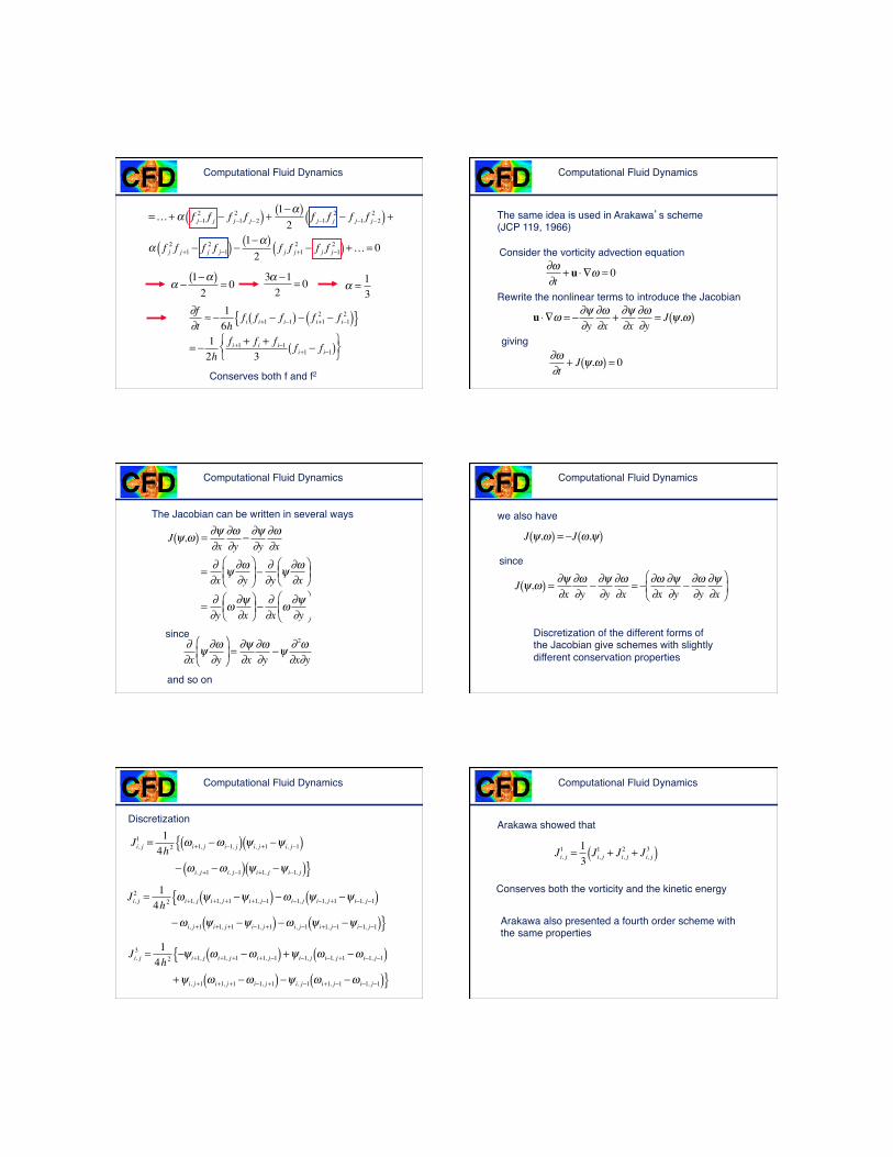
Conserves both f and f2!


The same idea is used in Arakawa’s scheme (JCP 119, 1966)!

�

∂ω∂t

+ u ⋅ ∇ω = 0

�

u ⋅ ∇ω = −∂ψ∂y

∂ω∂x

+ ∂ψ∂x

∂ω∂y

= J ψ,ω( )

�

∂ω∂t

+ J ψ,ω( ) = 0

Consider the vorticity advection equation!

Rewrite the nonlinear terms to introduce the Jacobian!

giving!


�

J ψ,ω( ) = ∂ψ∂x

∂ω∂y

− ∂ψ∂y

∂ω∂x

= ∂∂x

ψ ∂ω∂y

⎛

⎝ ⎜

⎞

⎠ ⎟ −

∂∂y

ψ ∂ω∂x

⎛ ⎝ ⎜

⎞ ⎠ ⎟

= ∂∂y

ω ∂ψ∂x

⎛ ⎝ ⎜

⎞ ⎠ ⎟ −

∂∂x

ω ∂ψ∂y

⎛

⎝ ⎜

⎞

⎠ ⎟

�

∂∂x

ψ ∂ω∂y

⎛

⎝ ⎜

⎞

⎠ ⎟ = ∂ψ

∂x∂ω∂y

−ψ ∂ 2ω∂x∂y

since!

and so on!

The Jacobian can be written in several ways!


�

J ψ,ω( ) = −J ω,ψ( )we also have!

�

J ψ,ω( ) = ∂ψ∂x

∂ω∂y

− ∂ψ∂y

∂ω∂x

= − ∂ω∂x

∂ψ∂y

− ∂ω∂y

∂ψ∂x

⎛

⎝ ⎜

⎞

⎠ ⎟

since!

Discretization of the different forms of the Jacobian give schemes with slightly different conservation properties !


�

Ji, j1 = 1

4h2ω i+1, j −ω i−1, j( ) ψ i, j+1 −ψ i, j−1( ){

− ω i, j+1 −ω i, j−1( ) ψi+1, j −ψ i−1, j( )}

Discretization!

�

Ji, j2 = 1

4h2ω i+1, j ψi+1, j+1 −ψ i+1, j−1( ){ −ω i−1, j ψ i−1, j+1 −ψ i−1, j−1( )−ω i, j+1 ψ i+1, j+1 −ψ i−1, j+1( ) −ω i, j−1 ψi+1, j−1 −ψ i−1, j−1( )}

�

Ji, j3 = 1

4h2−ψi+1, j ω i+1, j+1 −ω i+1, j−1( ){ +ψ i−1, j ω i−1, j+1 −ω i−1, j−1( )

+ψi, j+1 ω i+1, j+1 −ω i−1, j+1( ) −ψ i, j−1 ω i+1, j−1 −ω i−1, j−1( )}


Arakawa showed that!

Conserves both the vorticity and the kinetic energy!

�

Ji, j1 = 1

3Ji, j1 + Ji, j

2 + Ji, j3( )

Arakawa also presented a fourth order scheme with the same properties!


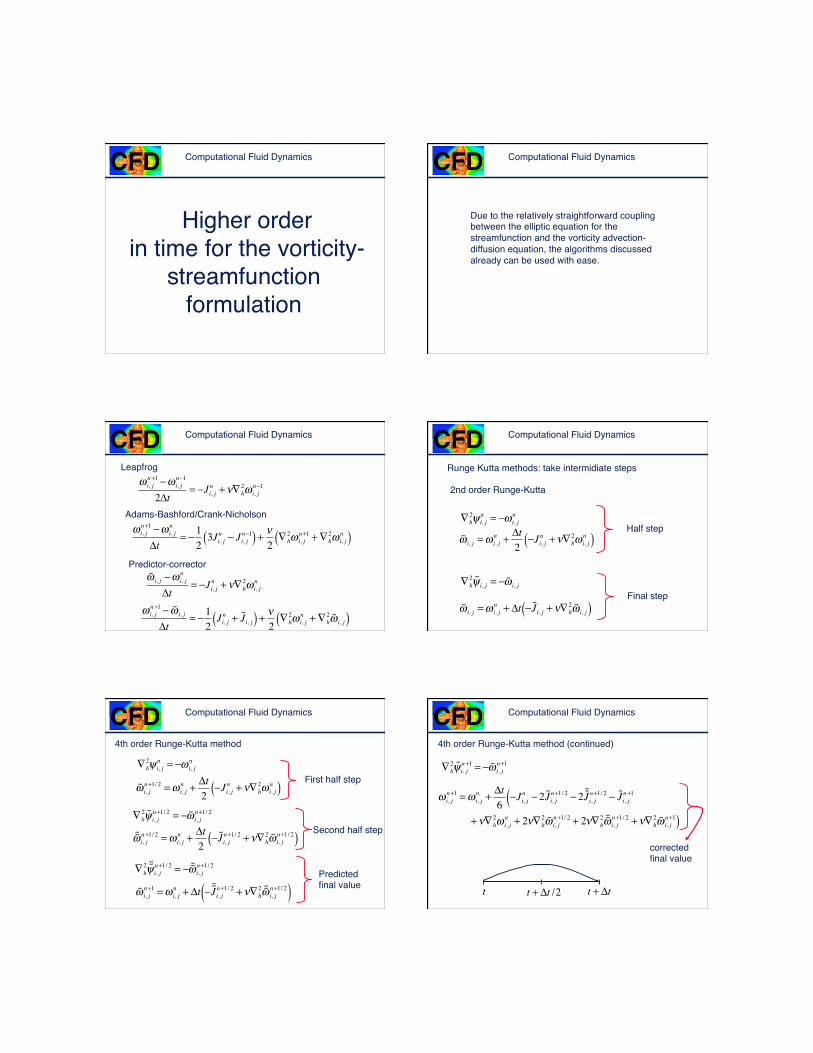
Higher order!in time for the vorticity-

streamfunction formulation !


Due to the relatively straightforward coupling between the elliptic equation for the streamfunction and the vorticity advection-diffusion equation, the algorithms discussed already can be used with ease.!


�

ω i, jn+1 −ω i, j

n−1

2Δt= −Ji, j

n + ν∇h2ω i, j

n−1

Leapfrog!

�

ω i, jn+1 −ω i, j

n

Δt= − 1

23Ji, j

n − Ji, jn−1( ) + ν

2∇h2ω i, j

n+1 + ∇h2ω i, j

n( )Adams-Bashford/Crank-Nicholson!

Predictor-corrector!

�

ω i, jn +1 − ˜ ω i, j

Δt= − 1

2Ji, j

n + ˜ J i, j( ) + ν2

∇h2ω i, j

n + ∇h2 ˜ ω i, j( )

�

˜ ω i, j −ω i, jn

Δt= −Ji, j

n + ν∇h2ω i, j

n


2nd order Runge-Kutta!

�

˜ ω i, j = ω i, jn + Δt

2−Ji, j

n + ν∇h2ω i, j

n( )

Runge Kutta methods: take intermidiate steps!

�

∇h2ψi, j

n = −ω i, jn

�

∇h2 ˜ ψ i, j = − ˜ ω i, j

�

˜ ω i, j = ω i, jn + Δt − ˜ J i, j + ν∇h

2 ˜ ω i, j( )

Half step!

Final step!


4th order Runge-Kutta method!

�

˜ ω i, jn+1/ 2 = ω i, j

n + Δt2

−Ji, jn + ν∇h

2ω i, jn( )

�

∇h2ψi, j

n = −ω i, jn

�

∇h2 ˜ ˜ ψ i, j

n+1/ 2 = − ˜ ˜ ω i, jn+1/ 2

�

˜ ω i, jn +1 = ω i, j

n + Δt − ˜ ˜ J i, jn +1/ 2 + ν∇h

2 ˜ ˜ ω i, jn +1/ 2( )

First half step!

Predicted final value!

�

∇h2 ˜ ψ i, j

n+1/ 2 = − ˜ ω i, jn+1/ 2

�

˜ ˜ ω i, jn +1/ 2 = ω i, j

n + Δt2

− ˜ J i, jn +1/ 2 + ν∇h

2 ˜ ω i, jn +1/ 2( ) Second half step!


4th order Runge-Kutta method (continued)!

�

ω i, jn +1 = ω i, j

n + Δt6

−Ji, jn − 2 ˜ J i, j

n +1/ 2 − 2 ˜ ˜ J i, jn +1/ 2 − ˜ J i, j

n +1(+ ν∇h

2ω i, jn + 2ν∇h

2 ˜ ω i, jn +1/ 2 + 2ν∇h

2 ˜ ˜ ω i, jn +1/ 2 + ν∇h

2 ˜ ω i, jn +1)

corrected final value!

�

∇h2 ˜ ψ i, j

n+1 = − ˜ ω i, jn+1

�

t

�

t + Δt

�

t + Δt /2


Generating higher order methods for the Navier-Stokes equations in the vorticity/streamfunction form is relatively straight forward and any method developed for the advection diffusion equation can be used without much difficulty!


Boundary Conditions for Inflow and Outflow!Compact schemes!Conservation of energy!Higher order in time for ! the ψ-ω formulation!

Outline!

Boundary conditions Inﬂow and outﬂowgtryggva/CFD-Course/2013-Lecture-22.pdf · Periodic...

Documents

Transcript of Boundary conditions Inﬂow and outﬂowgtryggva/CFD-Course/2013-Lecture-22.pdf · Periodic...