SUBLINEARLY MORSE BOUNDARY II: PROPER GEODESIC SPACES

YULAN QING, KASRA RAFI, AND GIULIO TIOZZO

Abstract. We build an analogue of the Gromov boundary for any proper geodesic metric space,hence for any finitely generated group. More precisely, for any proper geodesic metric space X andany sublinear function κ, we construct a boundary for X, denoted ∂κX, that is quasi-isometricallyinvariant and metrizable. As an application, we show that when G is the mapping class group ofa finite type surface, or a relatively hyperbolic group, then with minimal assumptions the Poissonboundary of G can be realized on the κ-Morse boundary of G equipped the word metric associatedto any finite generating set.

1. Introduction

In this paper, we construct an analogue of the Gromov boundary for a general proper geodesicmetric space. That is, a notion of a boundary at infinity that is invariant under quasi-isometry,has good topological properties and is as large as possible. Our guiding principle is that, movingfrom the setting of Gromov hyperbolic spaces to general metric spaces, most key arguments stillgo through if we replace uniform bounds with sublinear bounds (with respect to distance to somebase point). Examples of this philosophy have appeared in the literature before, for example in[Dru00, Kar11, EFW12, EFW13, ACGH17, EMR18]. In a prequel to this paper [QRT19], such aboundary was constructed in the setting of CAT(0) metric spaces.

Statement of Results. Let (X, dX) be a proper, geodesic metric space with a base point o. Recallthat, when X is Gromov hyperbolic, the Gromov boundary of X is the set of equivalence classesof quasi-geodesic rays emanating from o, equipped with the cone topology. Two quasi-geodesicrays are considered equivalent if they stay within bounded distance from each other. In a Gromovhyperbolic space, every quasi-geodesic ray β is Morse: that is, any other quasi-geodesic segment γwith endpoints on β stays in a bounded neighborhood of β.

Similarly, we consider quasi-geodesic rays in X (rays are always assumed to be emanating fromo). Roughly speaking, we say a quasi-geodesic ray β is sublinearly Morse if any other quasi-geodesic segment γ with endpoints sublinearly close to β stays in a sublinear neighborhood of β(see Definition 3.2 for the precise definition). We group the set of sublinearly Morse quasi-geodesicrays into equivalence classes by setting quasi-geodesic rays α and β to be equivalent if they staysublinearly close to each other. We call the set of equivalence classes of sublinearly Morse quasi-geodesic rays, equipped with a coarse version of the cone topology, the sublinearly Morse boundaryof X.

In fact, the above construction works for any given sublinear function κ : [0,∞)→ [1,∞), whereκ is a concave, increasing function with

limt→∞

κ(t)

t= 0.

Then, we define the κ-Morse boundary ∂κX to be the space of equivalence classes of κ-Morse quasi-geodesic rays equipped with the coarse cone topology (see Definition 4.1). We obtain a possiblylarge family of boundaries for X, each associated to a different sublinear function κ.

Date: November 6, 2020.1

We show that ∂κX is metrizable and invariant under quasi-isometries; moreover, κ-boundariesassociated to different sublinear functions are topological subspaces of each other.

Theorem A. Let X be a proper, geodesic metric space, and let κ be a sublinear function. Then weconstruct a topological space ∂κX with the following properties:

(1) (Metrizability) The spaces ∂κX and X ∪∂κX are metrizable, and X ∪∂κX is a bordificationof X;

(2) (QI-invariance) Every (k,K)-quasi-isometry Φ: X → Y between proper geodesic metricspaces induces a homeomorphism Φ? : ∂κX → ∂κY ;

(3) (Compatibility) For sublinear functions κ and κ′ where κ ≤ c · κ′ for some c > 0, wehave ∂κX ⊂ ∂κ′X where the topology of ∂κX is the subspace topology. Further, letting∂X :=

⋃κ ∂κX, we obtain a quasi-isometry invariant topological space that contains all

∂κX as topological subspaces. We call ∂X the sublinearly Morse boundary of X.

Note that from QI-invariance it follows that ∂κX and ∂X do not depend on the base point o.Moreover, it also implies that the κ-Morse boundary of a finitely generated group G is independentof the generating set. Thus ∂κG and ∂G are well defined.

We now argue that, in different settings, the κ-Morse boundary ∂κX is large for an appropriatechoice of κ. Recall that the Poisson boundary is the maximal boundary from the measurable pointof view (see Section 6). In this paper, we let G be either a mapping class group or a relativelyhyperbolic group and X be a Cayley graph of G and show that ∂κX is a topological model for thePoisson boundary of (G,µ) associated to any non-elementary finitely supported measure µ.

In fact, we show the following general criterion: if almost every sample path of the random walkdriven by µ sublinearly tracks a κ-Morse geodesic, then the κ-Morse boundary can be identifiedwith the Poisson boundary. The following result was obtained in collaboration with Ilya Gekhtman.

Theorem B. Let G be a finitely generated group, and let (X, dX) be a Cayley graph of G. Let µbe a probability measure on G with finite first moment with respect to dX , such that the semigroupgenerated by the support of µ is a non-amenable group. Let κ be a sublinear function, and supposethat for almost every sample path ω = (wn), there exists a κ-Morse geodesic ray γω such that

(1) limn→∞

dX(wn, γω)

n= 0.

Then almost every sample path converges to a point in ∂κX, and moreover the space (∂κX, ν), whereν is the hitting measure for the random walk, is a model for the Poisson boundary of (G,µ).

For comparison, recall that the visual boundary of CAT(0) spaces is not invariant by quasi-isometries [CK00]. The Gromov boundary [Gro87], on the other hand, is QI-invariant, but onlydefined if the group is hyperbolic; a natural generalization is the Morse boundary [Cor18], which isalways well-defined and QI-invariant, but very often it is too small: in particular, it has measurezero with respect to the hitting measure for most random walks on relatively hyperbolic groups[CDG20]. This is related to the fact that a typical sample path is expected to have unboundedexcursions in the peripherals.

Mapping class groups. Let S be a surface of finite hyperbolic type and Map(S) be the mappingclass group of S. Let dw be the word metric on Map(S) with respect to some finite generatingset. Then letting (X, dX) = (Map(S), dw) we can consider the κ-Morse boundary ∂κ Map(S) of themapping class group. We show the following characterization.

Theorem C. Let µ be a finitely supported, non-elementary probability measure on Map(S), and letp := 3 g(S)− 3 + b(S) be the complexity of S. Then for κ(t) = logp(t), we have:

(1) Almost every sample path (wn) converges to a point in ∂κ Map(S);2

(2) The κ-Morse boundary (∂κ Map(S), ν) is a model for the Poisson boundary of (Map(S), µ)where ν is the hitting measure associated to the random walk driven by µ.

The proof uses the machinery of curve complexes introduced by Masur-Minsky [MM00], as wellthe study of random walks in mapping class groups carried by Maher [Mah10], [Mah12], Sisto[Sis17], Maher-Tiozzo [MT18] and Sisto-Taylor [ST19]. In particular, by [ST19], a typical samplepath makes logarithmic progress in each subsurface, which explains the function log(t), while p isrelated to the “depth" of the hierarchy paths in Map(S).

Moreover, we also obtain the following tracking result between geodesics and sample paths in themapping class group.

Theorem D. Let µ be a finitely supported, non-elementary probability measure on Map(S), and letp as above. Then, for almost every sample path there exists a κ-Morse geodesic ray γω in Map(S)such that

lim supn→∞

dw(wn, γω)

logp+1(n)< +∞.

This result improves the tracking result of Sisto [Sis17], where the tracking function is√n log n.

Sublinear tracking for random walks with respect to the Teichmüller metric was obtained in [Tio15].

Relatively hyperbolic groups. Now consider a finitely generated group G equipped with a wordmetric dw associated to a finite generating set. Recall that G is relatively hyperbolic with respectto a family of subgroups H1, . . . ,Hk if, after contracting the Cayley graph of G along Hi-cosets,the resulting graph equipped with the usual graph metric is Gromov hyperbolic. Further, Hi-cosetshave to satisfy the technical condition of bounded coset penetration. Similarly to above, we show:

Theorem E. Let G be a non-elementary relatively hyperbolic group, and let µ be a probabilitymeasure whose support is finite and generates G as a semigroup. Then for κ(t) = log(t), we have:

(1) Almost every sample path (wn) converges to a point in ∂κG;(2) The κ-Morse boundary (∂κG, ν) is a model for the Poisson boundary of (G,µ) where ν is

the hitting measure associated to the random walk driven by µ.

Remark 1.1. The proof of Theorem C also works in the setting of hierarchically hyperbolic spaces[BHS17]. Hierarchically hyperbolic spaces are a family of axiomatically defined spaces with proper-ties that are modelled after the mapping class groups. Hence, all the tools we use, such as subsurfaceprojections, distance formulas and the Bounded Geodesic Image Theorem also exist in the settingof hierarchically hyperbolic spaces.

Sublinearly Morse vs. Sublinearly Contracting. In the construction of the κ-Morse boundary∂κX, several different definitions are possible for the notion of a κ-Morse quasi-geodesic. The goal isalways to emulate the behavior of quasi-geodesics in a Gromov hyperbolic space but with sublinearerrors (instead of uniform additive errors).

The definition of κ-Morse given in this paper (Definition 3.2) is equivalent to the definition ofstrongly Morse in [QRT19]. Another natural condition is to require a quasi-geodesic ray β to beκ-weakly contracting (Definition 5.3): that is, that the projection of a ball disjoint from β to β hasa diameter that is bounded by a sublinear function of the distance of the center of the ball to theorigin.

In the setting of CAT(0) spaces, these two notions are equivalent ([QRT19, Theorem 3.8]), but thisis no longer true for general metric spaces. In the Appendix, we prove that κ-weakly contractingquasi-geodesics are always κ-Morse. The converse is known not to be the case in general: forexample, when κ is the constant function, a geodesic axis of a pseudo-Anosov element in the mappingclass group is always Morse [MM00], but not always strongly contracting [RV18]. However, κ-Morsequasi-geodesics are always κ′-weakly contracting for a larger sublinear function κ′:

3

Theorem F. Let X be a proper geodesic metric space, let κ be a sublinear function, and let β be aquasi-geodesic ray in X. Then:

(1) If β is κ-weakly contracting, it is κ-Morse;(2) There is a sublinear function κ′ such that if β is κ-Morse then it is κ′-weakly contracting.

The definition of κ-Morse we use in this paper is the one that matches our philosophical approachthe best, is the most flexible and makes the arguments simplest. Hence, we think it is the correctdefinition with minimal assumptions.

In some places, the same arguments as in [QRT19] apply directly, while in others new ideas areneeded; for the sake of brevity, we shall skip the proofs when the arguments are exactly the same.

History. The notion of a Morse geodesic is classical [Mor24], and much progress has been madein recent years using Morse geodesics to define boundaries of groups. In [Cor18], Cordes, inspiredby the sublinear boundary for CAT(0) spaces of Charney and Sultan [CS15], constructed the Morseboundary for all proper geodesic spaces, where a quasi-geodesic γ is Morse if there are uniformneighborhoods, with size depending on (q,Q), in which all (q,Q)-quasi-geodesic segments withendpoints on γ lie. The Morse boundaries are equipped with a direct limit topology and are invariantunder quasi-isometries. However, this space does not have good topological properties; for example,it is not first countable. Cashen-Mackay [CM19], following the work of Arzhantseva-Cashen-Gruber-Hume [ACGH17], defined a different topology on the Morse boundary. They showed that it isHausdorff and when there is a geometric action by a countable group, it is also metrizable; notethat Theorem A does not assume any geometric action. Another notion, more closely related toour definition of κ-Morse boundary, is defined by Kar [Kar11]: a geodesic space is asymptoticallyCAT(0) if balls of radius r are coarsely CAT(0) with an error of f(r), where the function f(r) issublinear. That is to say, a space is asymptotically CAT(0) if it has the same κ-Morse boundary asa CAT(0) space, where κ = f(r).

The definition of a contracting geodesic originates from [Mor24] and has been brought back toattention by [Gro87]. In [MM00] Masur-Minsky proved that axes of pseudo-Anosov elements arecontracting, and since then various versions of this condition have been discussed, in particular thenotions of strongly contracting and weakly contracting, see e.g. [Beh06], [BF09], [AK11], [ACT15],[Sis18], [Yan20], and [RV18]. Our definition of κ-weakly contracting is even weaker, and for thatreason it is expected to be generic with respect to many notions of genericity. For random walks,genericity of sublinearly contracting geodesics in relatively hyperbolic groups follows from [Sis17], inhierarchically hyperbolic groups it follows from [ST19] and in CAT(0) groups it follows from [GQR].For the counting measure, genericity of log-weakly contracting geodesics in RAAGs has been shownin [QT19].

The Poisson boundary of (G,µ) is trivial for all non-degenerate measures µ on abelian groups[CD60] and nilpotent groups [DM60]. Discrete subgroups of SL(d,R) are treated in [Fur63], wherethe Poisson boundary is related to the space of flags. For random walks on Lie groups, the study andthe description of the Poisson boundary was extensively developed in the 70’s and the 80’s by manyauthors, most notably Furstenberg. The Poisson boundary of some Fuchsian groups has also beendescribed by Series [Ser83] as being the limit set of the group. Kaimanovich [Kai94] identified thePoisson boundary of hyperbolic groups with their Gromov boundaries with the associated hittingmeasures. Karlsson and Margulis proved that visual boundaries of nonpositively curved spaces serveas models for their Poisson boundaries [KM99]. Kaimanovich and Masur [KM96, KM98] proved thatthe Poisson boundary of the mapping class group is the boundary of Thurston’s compactificationof Teichmüller space. Their description also runs for the Poisson boundary of the braid group; see[FM98].

4

Acknowledgement. Y.Q. thanks the University of Toronto for its hospitality in Fall 2020. K.R.is partially supported by NSERC. G.T. is partially supported by NSERC and the Alfred P. Sloanfoundation. This material is based upon work supported by the National Science Foundation underGrant No. DMS-1928930 while G.T. participated in a program hosted by the Mathematical SciencesResearch Institute in Berkeley, California, during the Fall 2020 semester. We thank Ilya Gekhtmanfor several useful conversations.

2. Preliminaries

Let (X, dX) be a proper, geodesic metric space, and let o ∈ X be a base point. Given a pointp ∈ X, we denote ‖p‖ := dX(o, p). Let α be a quasi-geodesic ray starting at o. For r > 0, let tr bethe first time where ‖α(tr)‖ = r and denote the point α(tr) with

αr := α(tr),

while the segment from α(0) to α(tr) will be denoted as

α|r := α([0, tr]).

We collect here the two basic geometric properties of the space that we need:

Lemma 2.1. Let (X, dX) be a proper, geodesic metric space. Then:• For any closed set Z ⊂ X and any point x ∈ X, there is a closed set πZ(x) of nearest pointsin Z to x. We refer to any point in πZ(x) as a nearest point projection from x to Z.• Any sequence of geodesics βn : [0, n] → X with β0 = o has a subsequence that convergesuniformly on compact sets to a geodesic ray β0 : [0,∞)→ X.

The following lemma about nearest point projections will be used several times.

Lemma 2.2. Let α, β be two quasi-geodesic rays starting at the base point o ∈ X. Let x be a pointon α, and let p be a nearest point projection of x onto β. Then we have

‖p‖ ≤ 2‖x‖.Proof. Note that, since p is a nearest point projection of x onto β and o belongs to β, we have

dX(x, p) ≤ dX(o, x).

Hence, by the triangle inequality,

‖p‖ = dX(o, p) ≤ dX(o, x) + dX(x, p) ≤ 2dX(o, x) = 2‖x‖.

2.1. Sublinear functions. In this paper, a sublinear function will be a function κ : [0,∞)→ [1,∞)such that

limt→∞

κ(t)

t= 0.

Moreover, we say that κ : [0,∞) → [1,∞) is a concave sublinear function if it is sublinear andmoreover it is increasing and concave.

Remark 2.3. The assumptions that κ is increasing and concave make certain arguments cleaner,otherwise they are not really needed. One can always replace any sublinear function κ with anothersublinear function κ so that κ(t) ≤ κ(t) ≤ C κ(t) for some constant C and κ is monotone increasingand concave. For example, define

κ(t) := supλκ(u) + (1− λ) · κ(v)

∣∣∣ 0 ≤ λ ≤ 1, u, v > 0, and λu+ (1− λ)v = t.

Lemma 2.4. If κ : [0,∞)→ [1,∞) is a concave sublinear function and λ > 1, then

κ(λt) ≤ λκ(t)

for any t ≥ 0.5

Proof. By concavity,

κ(t) = κ

(1

λλt+ (1− λ−1) · 0

)≥ 1

λκ(λt) + (1− λ−1) · κ(0) ≥ 1

λκ(λt)

from which the claim follows.

3. The κ-Morse boundary

We now introduce the definition of κ-Morse quasi-geodesic, which will be fundamental for ourconstruction. To set the notation, we say a quantity D is small compared to a radius r > 0 if

(2) D ≤ r

2κ(r).

We will fix once and for all a base point o ∈ X, and all quasi-geodesic rays we consider will bebased at o. Given a quasi-geodesic ray α and a constant m, we define

Nκ(α,m) :=x ∈ X : dX(x, α) ≤ m · κ(‖x‖)

.

The following observation will be useful.

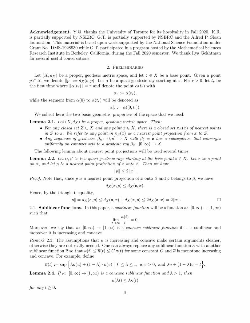
Lemma 3.1. Let β be a quasi-geodesic ray and α be a geodesic ray, both based at o ∈ X. Supposethat

β ⊆ Nκ(α,m)

for some function κ and some constant m. Then we also have

α ⊆ Nκ(β, 2m).

o α

β

yq

z

Figure 1. ‖y‖ = ‖z‖ and q ∈ πα(z) as in the proof of Lemma 3.1.

Proof. Let y ∈ α be a point and let r := ‖y‖. Let z ∈ β be a point such that ‖z‖ = r and let q bea nearest point projection of z to α. By assumption,

dX(z, q) ≤ m · κ(r).

On the other hand,

dX(y, q) = |‖y‖ − ‖q‖| since α is geodesic= |‖z‖ − ‖q‖|≤ dX(z, q) by triangle inequality.

Therefore we have

dX(y, β) ≤ dX(y, z) ≤ dX(y, q) + dX(q, z)

≤ 2dX(z, q)

≤ 2m · κ(r)

which completes the proof. 6

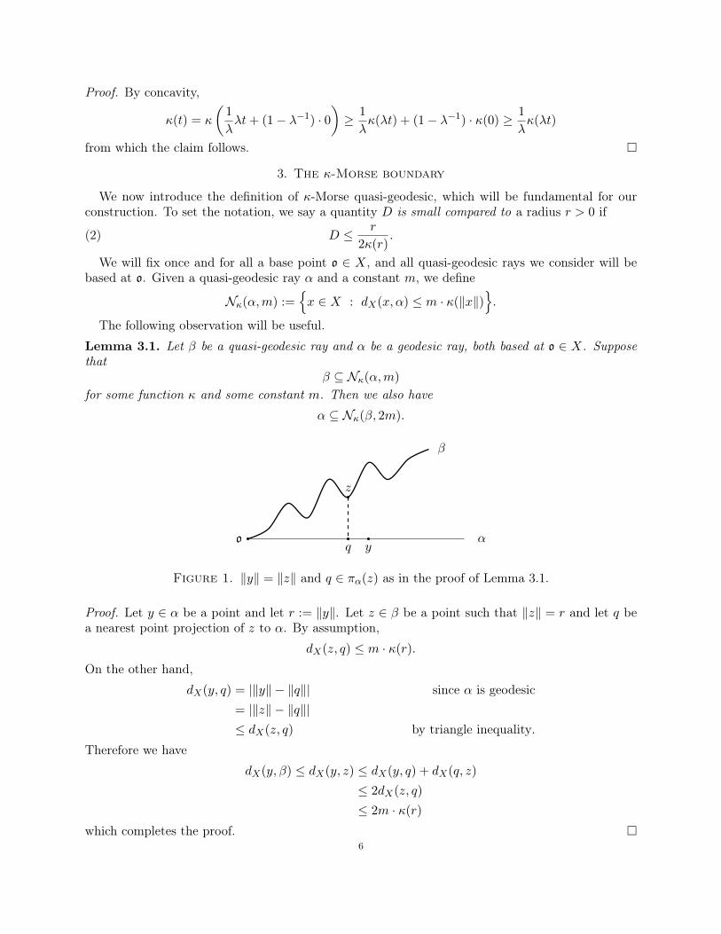
Definition 3.2. Let Z ⊆ X be a closed set, and let κ be a concave sublinear function. We say thatZ is κ-Morse if there exists a proper function mZ : R2 → R such that for any sublinear function κ′and for any r > 0, there exists R such that for any (q,Q)-quasi-geodesic ray β with mZ(q,Q) smallcompared to r, if

dX(βR, Z) ≤ κ′(R) then β|r ⊂ N(Z,mZ(q,Q)

)The function mZ will be called a Morse gauge of Z.

Note that we can always assume without loss of generality that maxq,Q ≤ mZ(q,Q), and wewill assume this in the following.

o Z

mZ(q,Q) · κ(r)

Rr

κ′(R)

βRβ

Figure 2. Definition of κ-Morse set Z: Every quasi-geodesic ray β has the propertythat there exists R(Z, r, q,Q, κ′), such that if βR is distance κ′(R) from Z, then β|ris in the neighborhood Nκ(Z,mZ(q,Q)).

3.1. Equivalence classes.

Definition 3.3. Given two quasi-geodesic rays α, β based at o, we say that β ∼ α if they sublinearlytrack each other: i.e. if

limr→∞

dX(αr, βr)

r= 0.

By the triangle inequality, ∼ is an equivalence relation on the space of quasi-geodesic rays basedat o, hence also on the space of κ-Morse quasi-geodesic rays.

Lemma 3.4. Let α be a κ-Morse quasi-geodesic rays with Morse gauge mα, and let β ∼ α be a(q,Q)-quasi-geodesic ray. Then:

(i) β is κ-Morse, and moreover

β ⊆ Nκ(α,mα(q,Q));

(ii) if in addition α is a geodesic ray, then

α ⊆ Nκ(β, 2mα(q,Q)).

Proof. (i) Define κ′(r) := dX(αr, βr). By definition of ∼, the function κ′ is sublinear, and moreover,for any R > 0,

dX(βR, α) ≤ κ′(R).

Hence, since α is κ-Morse, for any r we have

β|r ≤ mα(q,Q) · κ(r)

thus

(3) β ⊆ Nκ(α,mα(q,Q)),7

o α

β

β′

≤ κ′(R)

≤ κ′(R+ κ′(R))yt

qt

st

β′R

pR

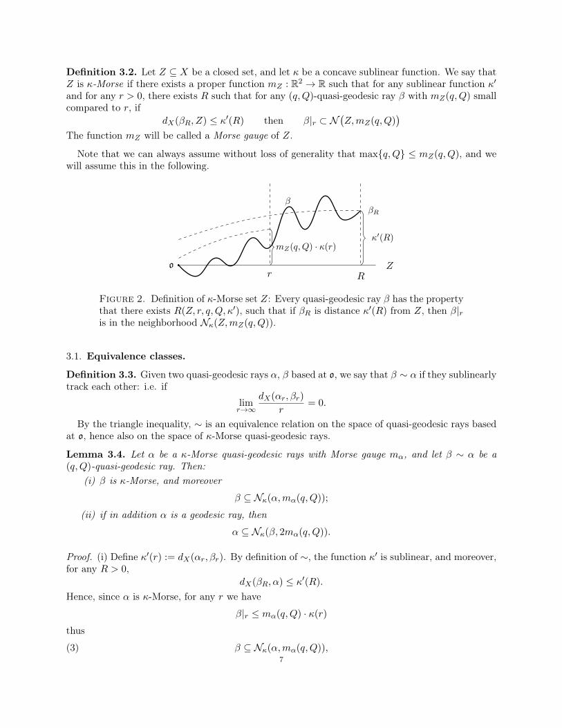
Figure 3. The setup in the proof of Lemma 3.4 (i).

which proves the second part of (i). Let us now prove that β is κ-Morse. Let κ′ be a sublinearfunction, let r > 0 and let β′ be a (q′, Q′)-quasi-geodesic ray such that

dX(β′R, β) ≤ κ′(R)

for some sufficiently large R. Let pR be a nearest point projection of β′R to β; by Lemma 2.2 wehave

‖pR‖ ≤ 2‖β′R‖ = 2R.

Then, by the triangle inequality and equation (3),

dX(β′R, α) ≤ dX(β′R, pR) + dX(pR, α)

≤ κ′(R) +mα(q,Q) · κ(‖pR‖)≤ κ′(R) +mα(q,Q) · κ(2R).

Since κ′′(R) := κ′(R) + m(q,Q) · κ(2R) is also a sublinear function, and since α is κ-Morse, thisimplies that

β|r ⊆ Nκ(α,mα(q′, Q′)).

Let yt be any point on β′ with ‖yt‖ = t ≤ r. By Lemma 2.2, if qt is a nearest point projection of ytto α, we have

‖qt‖ ≤ 2‖yt‖ = 2t.

Now, if q is a point on α and s is a nearest point projection of q to β, by the triangle inequality andthe Morse property,

‖q‖ ≥ ‖s‖ − dX(s, q) ≥ ‖s‖ −mα(q,Q) · κ(‖s‖).Moreover, by Lemma 2.2, ‖s‖ ≤ 2‖q‖, hence by concavity

dX(s, q) ≤ mα(q,Q) · κ(‖s‖) ≤ 2mα(q,Q) · κ(‖q‖).

Now, if st is a nearest point projection of qt to β, the above estimate yields

dX(qt, st) ≤ 2mα(q,Q) · κ(‖qt‖)≤ 4mα(q,Q) · κ(t)

hence, putting everything together,

dX(yt, β) ≤ dX(yt, qt) + dX(qt, st)

≤ mα(q′, Q′) · κ(t) + 4mα(q,Q) · κ(t)

which, by setting mβ(q′, Q′) := mα(q′, Q′) + 4mα(q,Q), proves the claim.(ii) It follows immediately from (i) and Lemma 3.1.

8

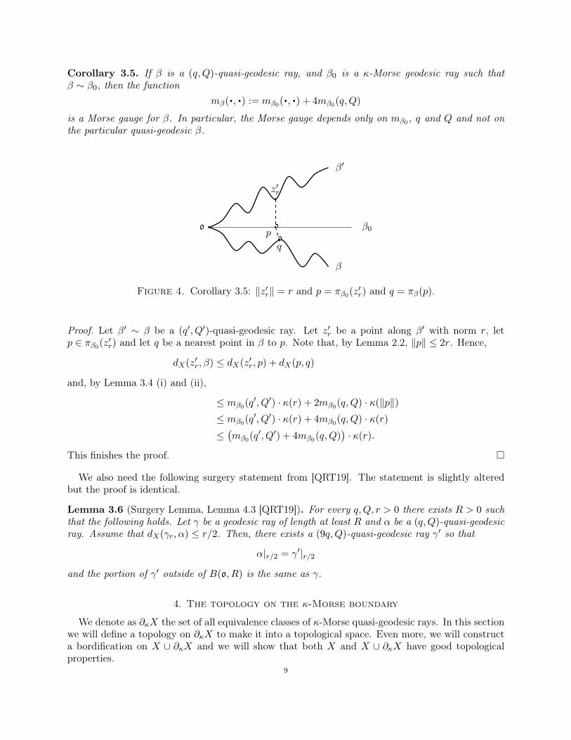
Corollary 3.5. If β is a (q,Q)-quasi-geodesic ray, and β0 is a κ-Morse geodesic ray such thatβ ∼ β0, then the function

mβ(, ) := mβ0(, ) + 4mβ0(q,Q)

is a Morse gauge for β. In particular, the Morse gauge depends only on mβ0, q and Q and not onthe particular quasi-geodesic β.

o β0

β′

β

p

q

z′r

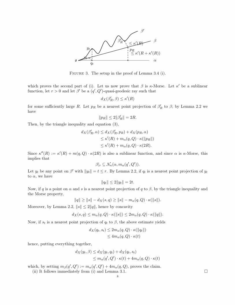
Figure 4. Corollary 3.5: ‖z′r‖ = r and p = πβ0(z′r) and q = πβ(p).

Proof. Let β′ ∼ β be a (q′, Q′)-quasi-geodesic ray. Let z′r be a point along β′ with norm r, letp ∈ πβ0(z′r) and let q be a nearest point in β to p. Note that, by Lemma 2.2, ‖p‖ ≤ 2r. Hence,

dX(z′r, β) ≤ dX(z′r, p) + dX(p, q)

and, by Lemma 3.4 (i) and (ii),

≤ mβ0(q′, Q′) · κ(r) + 2mβ0(q,Q) · κ(‖p‖)≤ mβ0(q′, Q′) · κ(r) + 4mβ0(q,Q) · κ(r)

≤(mβ0(q′, Q′) + 4mβ0(q,Q)

)· κ(r).

This finishes the proof.

We also need the following surgery statement from [QRT19]. The statement is slightly alteredbut the proof is identical.

Lemma 3.6 (Surgery Lemma, Lemma 4.3 [QRT19]). For every q,Q, r > 0 there exists R > 0 suchthat the following holds. Let γ be a geodesic ray of length at least R and α be a (q,Q)-quasi-geodesicray. Assume that dX(γr, α) ≤ r/2. Then, there exists a (9q,Q)-quasi-geodesic ray γ′ so that

α|r/2 = γ′|r/2

and the portion of γ′ outside of B(o, R) is the same as γ.

4. The topology on the κ-Morse boundary

We denote as ∂κX the set of all equivalence classes of κ-Morse quasi-geodesic rays. In this sectionwe will define a topology on ∂κX to make it into a topological space. Even more, we will constructa bordification on X ∪ ∂κX and we will show that both X and X ∪ ∂κX have good topologicalproperties.

9

4.1. Bordification. Let β be a κ-Morse quasi-geodesic ray based at o and let mβ be a Morse gaugefor β.

Definition 4.1. We define the set U(β, r) ⊆ X ∪ ∂κX as follows.• An equivalence class a ∈ ∂κX belongs to U(β, r) if, for any (q,Q)-quasi-geodesic ray α ∈ a,where mβ(q,Q) is small compared to r (in the sense of Equation 2), we have the inclusion

α|r ⊆ Nκ(β,mβ(q,Q)

).

• A point p ∈ X belongs to U(β, r) if dX(o, p) ≥ r and, for every (q,Q)-quasi-geodesic αbetween o and p where mβ(q,Q) is small compared to r, we have

α|r ⊆ Nκ(β,mβ(q,Q)

).

We denote U(β, r) ∩ ∂κX by ∂U(β, r).

We now verify the following basic properties of U(β, r).

Lemma 4.2. Let β be a quasi-geodesic ray which belongs to the class b. Then:(1) There exists a (not necessarily unique) geodesic ray in the class b;(2) The class b belongs to U(β, r) for any r > 0;(3)

⋂r>0 U(β, r) = b;

(4) If β1 ∼ β2 are two κ-Morse quasi-geodesic rays, for any r1 > 0, there exists r2 > 0 such that

U(β1, r1) ⊇ U(β2, r2).

Proof. (1) Consider the geodesic segment βn connecting o and β(n) for n = 1, 2, 3.... The sequenceof geodesic segments has a convergent subsequence converging to a geodesic ray β′ by Arzelá-Ascoli.Since β is κ-Morse, βn ⊂ Nκ

(β,mβ(1, 0)

). Therefore the same is true for β′ and hence β′ belongs

to the class b.(2) If β′ is a (q,Q)-quasi-geodesic ray which belongs to b, then by Lemma 3.4

β′ ⊆ Nκ(β,mβ(q,Q))

hence alsoβ′|r ⊆ Nκ(β,mβ(q,Q))

for any r > 0, as needed.(3) Let c ∈ ∂κX be a class which belongs to U(β, r) for any r, let (q′, Q′) be the quasi-geodesic

constants of β, and let γ ∈ c be a (q,Q)-quasi-geodesic ray. Let β′ be a geodesic ray based at owith β′ ∼ β.

Take y ∈ γ such that ‖y‖ = r. Then, by assumption,

γ|r ⊆ Nκ(β,mβ(q,Q)

),

for any r. Hence, if p is a nearest point projection of y onto β, we have

dX(y, β) = dX(y, p) ≤ mβ(q,Q) · κ(r).

Moreover, by Lemma 2.2, we have ‖p‖ ≤ 2‖y‖ = 2r and, by Lemma 3.4 (i), we have

dX(y, β′) ≤ dX(y, p) + dX(p, β′)

≤ mβ(q,Q) · κ(r) + 2mβ′(q′, Q′) · κ(r).

Settingmβ′(q,Q) := mβ(q,Q) + 2mβ′(q′, Q′),

we get,γ|r ⊆ Nκ

(β′, mβ′(q,Q)

),

for any r > 0.10

Let now pr be a nearest point projection of γr to β′. Then

|dX(o, pr)− r| = |dX(o, pr)− dX(o, γr)| ≤ dX(γr, pr) ≤ mβ′(q,Q) · κ(r).

Since β′ is geodesic, we have

dX(pr, β′r) = |dX(o, pr)− r| ≤ mβ′(q,Q) · κ(r)

anddX(γr, β

′r) ≤ dX(γr, pr) + dX(pr, β

′r) ≤ 2mβ′(q,Q) · κ(r).

But κ(r) is sublinear, therefore,

limr→∞

dX(γr, β′r)

r= 0

which implies γ ∈ b and c = b. Finally, since p ∈ U(β, r) implies dX(o, p) ≥ r, the intersection⋂r>0 U(β, r) does not contain any point of X.(4) Let β1 be a (q1, Q1)-quasi-geodesic ray, β2 a (q2, Q2)-quasi-geodesic ray with β1 ∼ β2, and

let r1 > 0. For r > 0, let a ∈ U(β2, r), and pick α ∈ a be a (q,Q)-quasi-geodesic ray such thatmβ2(q,Q) is small compared to r. By definition of U(β2, r) we have

dX(αr, β2) ≤ mβ2(q,Q) · κ(r).

Let pr be a nearest point projection of αr to β2. By Lemma 2.2,

‖pr‖ ≤ 2r.

Moreover, by Lemma 3.4 (i),

dX(pr, β1) ≤ κ(‖pr‖)mβ1(q2, Q2) ≤ 2mβ1(q2, Q2) · κ(r)

hence

(4) dX(αr, β1) ≤ mβ2(q,Q) · κ(r) + 2mβ1(q2, Q2) · κ(r).

Now, if we takeκ′(r) := mβ2(q,Q) · κ(r) + 2mβ1(q2, Q2) · κ(r),

by Definition 3.2, there exists r2 such that (4) for r = r2 implies

α|r1 ⊆ Nκ(β1,mβ1(q,Q)

)hence a ∈ U(β1, r1), as required.

We now verify that a sequence of points of X that sublinearly tracks a quasi-geodesic ray γ,converges to the class of γ in ∂κX.

Lemma 4.3. Let γ ∈ c be a κ-Morse quasi-geodesic ray based at o ∈ X and let (xn) ⊆ X be asequence of points with ‖xn‖ → ∞. Moreover, suppose that there exists a constant C > 0 such that

(5) dX(xn, γ) ≤ C · κ(‖xn‖)

for all n. Then the sequence (xn) converges to c in the topology of X ∪ ∂κX.

Proof. In order to show the claim, we need to prove that for any quasi-geodesic ray β ∈ c and anyr > 0 there exists n0 such that for all n ≥ n0 we have

xn ∈ U(β, r).

Equivalently, we need to show that, for any r and any (q,Q)-quasi-geodesic segment α joining oand xn with mβ(q,Q) small with respect to r, we have

α|r ⊆ Nκ(β,mβ(q,Q)).11

Let pn be a nearest point projection of xn onto γ; by Lemma 2.2, ‖pn‖ ≤ 2‖xn‖. Now, by (5) andLemma 3.4,

dX(xn, β) ≤ dX(xn, pn) + dX(pn, β)

≤ C · κ(‖xn‖) + 2mβ(q′, Q′) · κ(‖xn‖)

where (q′, Q′) are the quasi-geodesic constants of γ. Note moreover that β is κ-Morse by Lemma3.4. Hence, consider the sublinear function

κ′(r) :=(C + 2mβ(q′, Q′)

)· κ(r)

and apply the definition of κ-Morse, obtaining R such that if dX(xn, β) ≤ κ′(R) then α|r ⊆Nκ(β,mβ(q,Q)). Thus, if we choose n0 so that ‖xn‖ ≥ R for all n ≥ n0, the definition of κ-Morse implies the following as needed,

α|r ⊆ Nκ(β,mβ(q,Q)).

We now show that the sets U(β, r) and ∂U(β, r) as a neighborhood basis to define topologies onX ∪ ∂κX and ∂κX.

Definition 4.4. Given an equivalence class b, we define the set B(b) as the set of subsets V ⊆X ∪ ∂κX such that there exists β ∈ b and r > 0 for which U(β, r) ⊆ V. Let ∂B(b) be the set ofsubsets of ∂κX of the form V ∩ ∂κX where V ∈ B(b), equivalently a set in ∂B(b) contains a set ofthe form ∂U(β, r). Also, for x ∈ X, define B(x) to be the set of subsets V of X such that V containsa ball B(x, r) of radius r centered at x.

Lemma 4.5. For every b ∈ ∂κX, the set B(b) satisfies the following properties:(i) Every subset of X ∪ ∂κX which contains a set belonging to B(b) itself belongs to B(b);(ii) Every finite intersection of sets of B(b) belongs to B(b);(iii) The element b is in every set of B(b);(iv) If V ∈ B(b) then there is W ∈ B(b) such that, for every a ∈ W, we have V ∈ B(a).

Furthermore, the same is true for subsets of ∂B(b) and B(x).

Proof. We prove the Lemma for B(b). The proof for ∂B(b) is identical. The proof for B(x) isimmediate from the fact that the open balls in X define a neighborhood basis for X.(i) This is immediate from the definition of B(b).(ii) It is enough to show that, for β1, . . . , βk ∈ b and r1, . . . , rk > 0, the intersection

U(β1, r1) ∩ U(β2, r2) ∩ · · · ∩ U(βk, rk),

belongs to B(b). By Lemma 4.2 (4), for any i = 1, . . . , k there exists Ri such that

U(βi, ri) ⊇ U(β1, Ri).

Thus, if we set

r := max1≤i≤k

Ri we havek⋂i=1

U(βi, ri) ⊇ U(β1, r)

and hence the intersection belongs to B(b).(iii) Established by Lemma 4.2 (2).(iv) We need to prove the following claim.

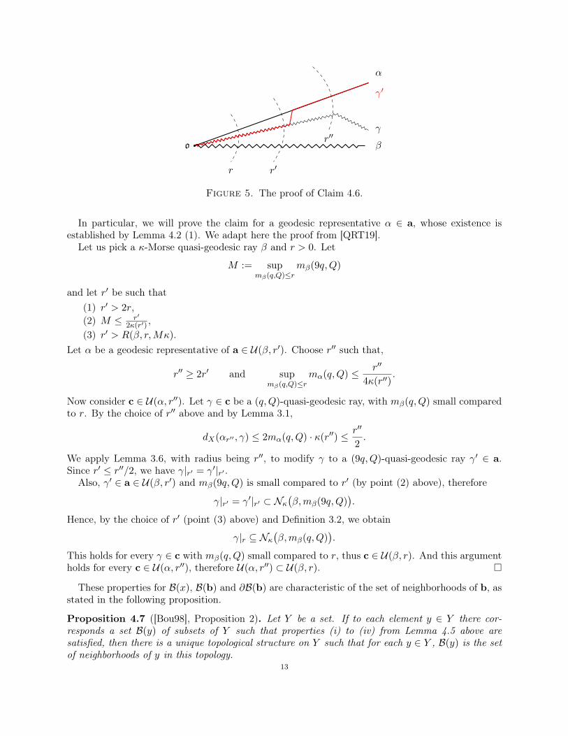
Claim 4.6. For any U(β, r), there exists r′ (usually larger than r) such that if a ∈ U(β, r′) thenthere exists r′′ (depending on α and r′ but not on β) such that U(α, r′′) ⊆ U(β, r) for some αrepresentative of a.

12

o β

α

γ′

γ

r r′

r′′

Figure 5. The proof of Claim 4.6.

In particular, we will prove the claim for a geodesic representative α ∈ a, whose existence isestablished by Lemma 4.2 (1). We adapt here the proof from [QRT19].

Let us pick a κ-Morse quasi-geodesic ray β and r > 0. Let

M := supmβ(q,Q)≤r

mβ(9q,Q)

and let r′ be such that(1) r′ > 2r,(2) M ≤ r′

2κ(r′) ,(3) r′ > R(β, r,Mκ).

Let α be a geodesic representative of a ∈ U(β, r′). Choose r′′ such that,

r′′ ≥ 2r′ and supmβ(q,Q)≤r

mα(q,Q) ≤ r′′

4κ(r′′).

Now consider c ∈ U(α, r′′). Let γ ∈ c be a (q,Q)-quasi-geodesic ray, with mβ(q,Q) small comparedto r. By the choice of r′′ above and by Lemma 3.1,

dX(αr′′ , γ) ≤ 2mα(q,Q) · κ(r′′) ≤ r′′

2.

We apply Lemma 3.6, with radius being r′′, to modify γ to a (9q,Q)-quasi-geodesic ray γ′ ∈ a.Since r′ ≤ r′′/2, we have γ|r′ = γ′|r′ .

Also, γ′ ∈ a ∈ U(β, r′) and mβ(9q,Q) is small compared to r′ (by point (2) above), therefore

γ|r′ = γ′|r′ ⊂ Nκ(β,mβ(9q,Q)

).

Hence, by the choice of r′ (point (3) above) and Definition 3.2, we obtain

γ|r ⊆ Nκ(β,mβ(q,Q)

).

This holds for every γ ∈ c with mβ(q,Q) small compared to r, thus c ∈ U(β, r). And this argumentholds for every c ∈ U(α, r′′), therefore U(α, r′′) ⊂ U(β, r).

These properties for B(x), B(b) and ∂B(b) are characteristic of the set of neighborhoods of b, asstated in the following proposition.

Proposition 4.7 ([Bou98], Proposition 2). Let Y be a set. If to each element y ∈ Y there cor-responds a set B(y) of subsets of Y such that properties (i) to (iv) from Lemma 4.5 above aresatisfied, then there is a unique topological structure on Y such that for each y ∈ Y , B(y) is the setof neighborhoods of y in this topology.

13

Thus we now use the sets ∂B(b) to equip ∂κX with a topological structure and use the sets B(b)and B(x) to equip X∪∂κX with a topological structure. Note that, since neighborhoods in ∂κX areintersections of neighborhoods of X ∪ ∂κX with ∂κX, we have that the inclusion ∂κX ⊂ X ∪ ∂κXis a topological embedding and X ∪ ∂κX is a bordification of X.

Recall that a set is open if it contains a neighborhood of each of its points. Thus, a setW ⊆ ∂κXis open if for every b ∈ W there is β ∈ b and r > 0 such that ∂U(β, r) ⊂ W. A set W ⊂ X ∪ ∂κXis open if its intersection with both X and ∂κX is open.

4.2. Metrizability. We now establish the metrizability of the space ∂κX. To begin with, we needthe following property of the topology:

Lemma 4.8. For each κ-Morse quasi-geodesic ray β and r > 0, there exists a radius r′ > 0 suchthat for any point a ∈ ∂κX there exists r′′ > 0 (depending only on a and r′ and not on β) such thatfor every geodesic representative α0 ∈ a

U(α0, r′′) ∩ U(β, r′) 6= ∅ =⇒ a ∈ ∂U(β, r).

Similarly, for x ∈ X, let B(x, 1) be the ball of radius 1 centered at x. Then

B(x, 1) ∩ U(β, r′) 6= ∅ =⇒ x ∈ U(β, r).

Proof. This will be done using the Surgery Lemma 3.6. Pick a κ-Morse quasi-geodesic ray β andr > 0. Let Q := (q,Q) : mβ(q,Q) ≤ r

2κ(r), which is bounded by properness. Set

M := sup(q,Q)∈Q

mβ(9q,Q+ 1),

and r′ := R(β, r,Mκ). Let a ∈ ∂κX.By Corollary 3.5, there exists a constant u > 0 such that, for any geodesic ray ? ∈ a and any

(q,Q) ∈ Q we havem?(1, 0) + 3m?(q,Q) ≤ u.

Let R be the radius given in Lemma 3.6 associated to q,Q and 2r′, and let r′′ be large enough sothat

r′′ ≥ max2u · κ(r′′), 2r′, R.Let α0 be a geodesic ray in a. By assumption, there is a point c inside the intersection

c ∈ U(α0, r′′) ∩ U(β, r′).

If c ∈ ∂κX, let γ ∈ c be a geodesic ray in this class and if c ∈ X, let γ be a geodesic ray connectingo to c. In either case, γr′′ is well defined since, in the second case, dX(o, c) ≥ r′′. Let α ∈ a be a(q,Q)-quasi-geodesic ray with mβ(q,Q) small compared to r. To conclude a ∈ ∂U(β, r) we need toshow that α|r ⊂ Nκ(β,mβ(q,Q)).

Since c ∈ U(α0, r′′),

dX(γr′′ , α0) ≤ mα0(1, 0) · κ(r′′).

Let p ∈ πα0(γr′′). By definition of u and r′′, we have

‖p‖ ≤ r′′ +mα0(1, 0) · κ(r′′) ≤ 3

2r′′.

Therefore, Lemma 3.4 (ii) implies

dX(p, α) ≤ 2mα0(q,Q) · κ(p) ≤ 3mα0(q,Q) · κ(r′′).

Hence,dX(γr′′ , α) ≤ dX(γr′′ , p) + dX(p, α) ≤ u · κ(r′′) ≤ r′′/2.

14

We can now apply the Surgery lemma (Lemma 3.6) to α and γ with radius 2r′ to obtain a (9q,Q)-quasi-geodesic ray γ′ that is either in the class c if c ∈ ∂κX or ends in c if c ∈ X where γ′|r′ = α|r′ .Since c ∈ U(β, r′), we have

α|r′ = γ′|r′ ⊂ Nκ(β,mβ(9q,Q)

).

Observing that α|r′ is (q,Q)-quasi-geodesic and letting κ′ = mβ(9q,Q) · κ, the definition of r′ andκ-Morse implies that

α|r ⊂ Nκ(β,mβ(q,Q)

),

hence a ∈ U(β, r).To see the second assertion, assume y ∈ B(x, 1) ∩ U(β, r′). Let α be a (q,Q)-quasi-geodesic ray

ending at x where mβ(q,Q) is small compared to r. Let γ be a quasi-geodesic ray that is identical toα but at the last point in sent to y instead of x. Then γ is (q,Q+ 1)-quasi-geodesic. The definitionof r′ and κ-Morse implies that

α|r = γ|r ⊂ Nκ(β,mβ(q,Q)

),

hence x ∈ U(β, r).

Our method for establishing metrizability is via the following criterion.

Theorem 4.9 (Theorem 3, [Fri37]). Assume, for every point b of a topological space, there exists amonotonically decreasing sequence V1(b),V2(b), · · · ,Vi(b), · · · of neighborhoods whose intersectionis b and such that the following holds: For every point b of the neighborhood space and every integeri, there exists an integer j = j(b, i) > i such that if a is a point for which Vj(a) and Vj(b) have apoint in common then Vj(a) ⊂ Vi(b). Then the space is homeomorphic to a metric space.

We check this condition for ∂κX, using as neighborhoods Vi(b) the sets ∂U(β, r) previouslydefined.

Theorem 4.10. The space ∂κX is metrizable.

Proof. Our goal is to construct, for any i ∈ N and b ∈ ∂κX, neighborhoods Vi(b) which satisfy theconditions of Theorem 4.9.

Recall that, given a κ-Morse quasi-geodesic ray β and r > 0, we can define r′ as

r′(β, r) := R(β, r,Mκ),

as in the proof of Lemma 4.8. Note that both in Claim 4.6 and in Lemma 4.8, r′′ does not dependon β or r, but it depends on α, r′ and on

supmβ(q,Q)≤r

mα(q,Q).

Since q,Q ≤ mβ(q,Q) ≤ r ≤ r′, the maximum value of q,Q can be bounded in terms of α, r′,without referring to β or r. Hence, we can consider the function r′′(α, r′) such that both Claim 4.6and Lemma 4.8 hold.

For i ∈ N and a ∈ ∂κX, pick a geodesic representative α0 ∈ a and define

Vi(a) := ∂U(α0, ri(a)), where ri(a) := max(i, r′′(α0, i)

).

Also, given b and i, we define ρi(b) := r′(β0, ri(b)), and

j = j(b, i) :=⌈r′(β0, ρi(b)

)⌉,

where β0 is a geodesic representative in b. Assume Vj(a) and Vj(b) have a point in common, thatis,

∂U(α0, rj(a)

)∩ ∂U

(β0, rj(b)

)6= ∅.

15

Then, since rj(a) ≥ r′′(α0, j) and rj(b) ≥ j, by Lemma 4.8 we have

a ∈ ∂U(β0, ρi(b)

).

Now, Claim 4.6 implies

∂U(α0, r

′′(α0, ρi(b)))⊂ ∂U

(β0, ri(b)

).

But rj(a) = max(j, r′′(α0, j)

), thus

rj(a) ≥ r′′(α0, r′(β0, ρi(b))) ≥ r′′(α0, ρi(b)).

Therefore,

∂U(α0, rj(a)

)⊂ ∂U

(β0, ri(b)

),

which is to say Vj(a) ⊂ Vi(b). The theorem now follows from Theorem 4.9.

Similarly, we have

Theorem 4.11. The space X ∪ ∂κX is metrizable.

Proof. For i ∈ N and a ∈ ∂κX, let ri(a) be as in the proof of Theorem 4.10 and let

Vi(a) := U(α0, ri(a)).

For a point x ∈ X, we define Vi(x) := B(x, 1i ), the ball of radius 1i centered around x. Since

Lemma 4.8 holds for U(α0, ri(a)), the same proof as above works to check the conditions of Theo-rem 4.9 for any point b ∈ ∂κX.

For x ∈ X, we define j(x, i) := 3i. Then, if

Vj(x) ∩ Vj(y) 6= ∅,

there is a point z ∈ B(x, 13i) ∩B(y, 1

3i) and, by the triangle inequality,

Vj(y) = B(y, 13i) ⊂ B(x, 1i ).

Also, if Vj(x) ∩ Vj(b) 6= ∅, for x ∈ X and b ∈ ∂κX, then B(x, 1) ∩ U(β, rj(b)) 6= ∅. By thedefinition of j(b, i) and the second part of Lemma 4.8, this implies that

Vi(x) ⊂ B(x, 1) ⊂ U(β, ri(b)).

Again, the theorem follows from Theorem 4.9.

We are now ready to establish the quasi-isometric invariance of ∂κX.

Theorem 4.12. Consider proper geodesic metric spaces X and Y , let Φ: X → Y be a (k,K)-quasi-isometry and let κ be a concave sublinear function. Then Φ induces a homeomorphism Φ? : ∂κX →∂κY where, for b ∈ ∂sX and β ∈ b,

Φ?(b) = [Φ β],

where [·] denotes the equivalence class of a quasi-geodesic ray.

The proof is identical to the proof of Theorem 5.1 in [QRT19].16

4.3. The union of ∂κX. We note that topologies of different sublinear boundaries are compatible.

Proposition 4.13 (Proposition 4.10, [QRT19]). Let κ and κ′ be sublinear functions such that, forsome M > 0

κ′(t) ≤M · κ(t), ∀ t > 0.

Then, ∂κ′X ⊂ ∂κX as a subspace with the subspace topology.

The proof is identical to the proof of Proposition 4.10 from [QRT19] and is skipped. In view ofthis proposition, we can define the sublinearly Morse boundary of X as

∂X :=⋃κ

∂κX

which is the space of equivalence classes (up to sublinear fellow traveling) of all sublinearly Morsequasi-geodesic rays in X.

Remark 4.14. An open neighborhood V of a point b ∈ ∂X can be described as follows: assumeb ∈ ∂κX for some κ and choose a quasi-geodesic ray β ∈ b and a radius r > 0. Let Uκ(β, r) be theneighborhood of b in (X ∪ ∂κX) and let V be the closure of Uκ(β, r) in (X ∪ ∂X). That is, a pointin V ∩ ∂X is a class of κ′-sublinearly Morse quasi-geodesic rays for some κ′ different from κ thatare eventually contained in Uκ(β, r). The intersection V ∩X equals X ∩ Uκ(β, r).

Similar arguments as in Theorem 4.10 and Theorem 4.11 can be used to show that ∂X and(X ∪ ∂X) are also metrizable. We skip these, for the sake of brevity.

5. General projections and weakly sublinearly contracting sets

In order to deal with several applications to proper geodesic spaces (in particular, our applicationsto mapping class groups and relatively hyperbolic groups we shall see next), the usual notion ofnearest point projection may be ill-suited; for instance, it is well-known that nearest point projectionto a closed subset of a general (e.g., not hyperbolic) metric space need not be, even coarsely, well-defined.

Thus, we now introduce a more general notion of projection, which we call κ-projection, wherewe allow an additive error which is controlled by a sublinear function κ.

Let us denote as P(Z) the set of subsets of Z, and let us use the notation κ(x) := κ(‖x‖).

Definition 5.1. Let (X, dX) be a proper geodesic metric space and Z ⊆ X a closed subset, and letκ be a concave sublinear function. A map πZ : X → P(Z) is a κ-projection if there exist constantsD1, D2, depending only on Z and κ, such that for any points x ∈ X and z ∈ Z,

diamX(z ∪ πZ(x)) ≤ D1 · dX(x, z) +D2 · κ(x).

A κ-projection differs from a nearest point projection by a uniform multiplicative error and asublinear additive error.

Lemma 5.2. Given a closed set Z, we have for any x ∈ X

diamX(x ∪ πZ(x)) ≤ (D1 + 1) · dX(x, Z) +D2 · κ(x).

Proof. Let z ∈ Z be a point that realizes dX(x, Z). Then, by triangle inequality and applyingDefinition 5.1, we obtain

diamX(x ∪ πZ(x)) ≤ dX(x, z) + diamX(z ∪ πZ(x)) ≤ (D1 + 1) · dX(x, Z) +D2 · κ(x).

We now formulate a general definition of κ-weakly contracting with respect to a κ-projection πZ .17

Definition 5.3 (κ-weakly contracting). For a closed subspace Z of a metric space (X, dX) and aκ-projection πZ onto Z, we say Z is κ-weakly contracting with respect to πZ if there are constantsC1, C2, depending only on Z and κ, such that, for every x, y ∈ X

dX(x, y) ≤ C1 · dX(x, Z) =⇒ diamX

(πZ(x) ∪ πZ(y)

)≤ C2 · κ(x).

In the special case that πZ is the nearest point projection and C1 = 1, this property was calledκ-contracting in [QRT19]. It was shown in [QRT19] that, in the setting of CAT(0) spaces, this isstronger than the κ-Morse condition.

With respect to any projection we prove the following analogous statement of [QRT19, Theorem3.14]:

Theorem 5.4 (κ-weakly contracting implies sublinearly Morse). Let κ be a concave sublinear func-tion and let Z be a closed subspace of X. Let πZ be a κ-projection onto Z and suppose that Z isκ-weakly contracting with respect to πZ . Then, there is a function mZ : R2 → R such that, for everyconstant r > 0 and every sublinear function κ′, there is an R = R(Z, r, κ′) > 0 where the followingholds: Let η : [0,∞) → X be a (q,Q)-quasi-geodesic ray so that mZ(q,Q) is small compared to r,let tr be the first time ‖η(tr)‖ = r and let tR be the first time ‖η(tR)‖ = R. Then

dX(η(tR), Z

)≤ κ′(R) =⇒ η([0, tr]) ⊂ Nκ

(Z,mZ(q,Q)

).

The proof of this result is similar to the one in [QRT19], so we will postpone it to the appendix.Moreover, in the appendix we shall prove the following equivalence between κ-weakly contractingand κ-Morse (with a possibly different sublinear function) for any given closed set.

Theorem 5.5. Let (X, o) be a proper geodesic metric space with a fixed base point. Let Z be aclosed set and πZ be a κ-projection onto Z. The following hold:

(1) If Z is κ-weakly contracting with respect to πZ , then it is κ-Morse;(2) If Z is κ-Morse, then it is κ′-weakly contracting with respect to πZ for some sublinear

function κ′.

6. The Poisson boundary

We now show a general criterion (Theorem 6.2) for the κ-Morse boundary of a group to beidentified with its Poisson boundary.

Random walks. Let G be a locally compact, second countable group, with left Haar measure m,and let µ be a Borel probability measure on G, which we assume to spread-out, i.e. such that thereexists n for which µn is not singular w.r.t. m. Given µ, we consider the step space (GN, µN), whoseelements we denote as (gn). The random walk driven by µ is the G-valued stochastic process (wn),where for each n we define the product

wn := g1g2 . . . gn.

We denote as (Ω,P) the path space, i.e. the space of sequences (wn), where P is the measure inducedby pushing forward the measure µN from the step space. Elements of Ω are called sample paths andwill be also denoted as ω. Finally, let T : Ω→ Ω be the left shift on the path space.

Background on boundaries. Let us recall some fundamental definitions from the boundary the-ory of random walks. We refer to [Kai00] for more details. Let (B,A) be a measurable space onwhich G acts by measurable isomorphisms; a measure ν on B is µ-stationary if ν =

∫G g?ν dµ(g),

and in that case the pair (B, ν) is called a (G,µ)-space. Recall that a µ-boundary is a measurable(G,µ)-space (B, ν) such that there exists a T -invariant, measurable map bnd : (Ω,P) → (B, ν),called the boundary map.

18

Moreover, a function f : G → R is µ-harmonic if f(g) =∫G f(gh) dµ(h) for any g ∈ G. We

denote by H∞(G,µ) the space of bounded, µ-harmonic functions. One says a µ-boundary is thePoisson boundary of (G,µ) if the map

Φ : H∞(G,µ)→ L∞(B, ν)

given by Φ(f)(g) :=∫B f dg?ν is a bijection. The Poisson boundary (B, ν) is the maximal µ-

boundary, in the sense that for any other µ-boundary (B′, ν ′) there exists a G-equivariant, measur-able map p : (B, ν)→ (B′, ν ′).

Finally, a metric d on G is temperate if there exists C such that

m(g ∈ G : d(1, g) ≤ R) ≤ CeCR

for any R > 0. A measure µ has finite first moment with respect to d if∫G d(1, g) dµ(g) < +∞.

We will use the ray approximation criterion from [Kai00] for the Poisson boundary (for thisprecise version, see [FT18]).

Theorem 6.1. Let G be a locally compact, second countable group equipped with a temperate metricd, and let µ be a spread-out probability measure on G with finite first moment with respect to d. Let(B, λ) be a µ-boundary, and suppose that there exist maps πn : B → G for any n ∈ N such that foralmost every sample path ω = (wn) we have

(6) limn→∞

d(wn, πn(bnd(ω))

)n

= 0.

Then (B, λ) is the Poisson boundary of (G,µ).

The κ-Morse boundary is the Poisson boundary. We now apply this criterion to identify thePoisson boundary with the κ-Morse boundary. The following result was obtained in collaborationwith Ilya Gekhtman.

Theorem 6.2. Let G be a finitely generated group, and let (X, dX) be a Cayley graph of G. Let µbe a probability measure on G with finite first moment with respect to dX , such that the semigroupgenerated by the support of µ is a non-amenable group. Let κ be a concave sublinear function, andsuppose that for almost every sample path ω = (wn), there exists a κ-Morse geodesic ray γω suchthat

(7) limn→∞

dX(wn, γω)

n= 0.

Then almost every sample path converges to a point in ∂κX, and moreover the space (∂κX, ν), whereν is the hitting measure for the random walk, is a model for the Poisson boundary of (G,µ).

Proof. By the subadditive ergodic theorem and finite first moment, the limit

` := limn→∞

dX(o, wn)

n

exists almost surely and is constant, and ` > 0 since the group generated by the support of µ isnon-amenable (see [Woe00, Theorem 8.14 and Corollary 12.5]).

By Lemma 4.3 and Eq. (7), almost every sequence converges to [γω] ∈ ∂κX. Thus, we can definebnd : Ω→ ∂κX as

bnd(ω) := limn→∞

wn ∈ ∂κX,

which is T -invariant by definition. Moreover, bnd is measurable, since it is a pointwise limit of themeasurable functions wn with values in the space X ∪ ∂κX, which is metrizable by Theorem 4.11.Since G is finitely generated, any word metric dX on it is temperate.

19

Finally, by Eq. (7), almost every sample path sublinearly tracks a κ-Morse quasi-geodesic ray.Hence, let us define πn : ∂κX → G as πn(ξ) := αrn where α is a geodesic representative of the classof ξ ∈ ∂κX, and rn := b`nc.

Now, let ω ∈ Ω and γ = γω, and let pn be a nearest point projection of wn onto γ. By (7), wehave for almost every ω ∈ Ω

limn→∞

dX(wn, pn)

n→ 0,

hence also ‖pn‖n → `. Since pn and γrn lie on the same geodesic, this implies

dX(wn, γrn)

n≤ dX(wn, pn)

n+dX(pn, γrn)

n(8)

≤ dX(wn, pn)

n+|‖pn‖ − rn|

n→ 0 + `− ` = 0(9)

as n→∞. Finally, we obtaindX(wn, πn(bnd(ω)))

n=dX(wn, αrn)

n≤ dX(wn, γrn)

n+dX(γrn , αrn)

n,

and the first term tends to 0 because of (8), while the second term tends to 0 since α ∼ γ. Hence,by Theorem 6.1, (∂κX, ν) is a model for the Poisson boundary of (G,µ).

7. Boundaries of mapping class groups

In this section, we show that for an appropriate choice of κ, the κ-Morse boundary of any mappingclass group G = Map(S) can function as a topological model for the Poisson boundary of the pair(G,µ), where µ is any finitely-supported non-elementary measure.

We need to show that a generic sample path of such a random walk sublinearly tracks a κ-Morsequasi-geodesic ray. We will do so but showing that, in fact, the limiting quasi-geodesic ray isκ-weakly contracting.

7.1. Background on mapping class groups. Let S be a surface of finite hyperbolic type, let g(S)be its genus and b(S) the number of its boundary components. Let Map(S) denote the mappingclass group of S equipped with a word metric dw associated to a finite generating set. That is, weare in the setting where (X, dX) = (Map(S), dw).

Ending laminations. Let C(S) denote the curve graph of S (see [MM00] for definition and details).The curve graph is known to be δ-hyperbolic [MM00]. By [Kla98], the Gromov boundary of C(S)can be identified with the space of ending laminations EL(S), that is, the space of minimal fillinglaminations after forgetting the measure.

Subsurface projections. By a subsurface Y we always mean a connected π1-injective subsurfaceof S. For any subsurface Y let C(Y ) denote the curve graph of Y . Let ∂Y denote the multi-curveconsisting of all boundary components of Y . There is a projection map πY : C(S)→ C(Y ) definedon a subset of C(S) consisting of curves that intersect Y . This is essentially a map that sends acurve α ∈ C(S) to a set of curves in Y obtained from surgery between α and ∂Y . (Again, see[MM00] for details). The set πY (α) has a uniformly bounded diameter in C(Y ), independent of αor Y .

We can extend this projection to a map πY : Map(S) → C(Y ) as follows. Consider a set θ ofcurves on S that fill S. For example, following [MM00], we can assume θ is the union of a pantsdecomposition and a set of dual curves, one transverse to each curve in the pants decomposition.Then for x ∈ Map(S), define

πY (x) :=⋃α∈θ

πY (x(α)).

20

Again, the set πY (x) has a uniformly bounded diameter in C(Y ). For, x, y ∈ Map(S) define

dY (x, y) := diamC(Y )(πY (x) ∪ πY (y)).

In particular,dS(x, y) := diamC(S)(x(θ), y(θ)).

Also, when Y is an annulus with core curve α, we often use dα(x, y) instead of dY (x, y).In the discussion above, x and y can be replaced with an ending lamination ξ ∈ EL(S) since ξ

has non-trivial projection to every subsurface and πY (ξ) is always well-defined. That is, we define

dY (x, ξ) := diamC(Y )(πY (x), πY (ξ)).

The distance formula. In [MM00], it was shown that the word metric on Map(S) can be estimatedup to uniform additive and multiplicative constants by these subsurface projection distances. Tosimplify the exposition, we adopt the following notation. We fix S and a generating set for Map(S),and we say a constant M is uniform if it depends only on the topology of S and the generating set.For two quantities A and B, we write A ≺ B if there is a uniform constant M such that

A ≤M ·B +M.

We write A B if A ≺ B and B ≺ A and we use the notation O(A) for a quantity that has anupper bound of M ·A. Also, recall that, for K > 0,

bAcK :=

x x ≥ K0 x < K.

Now the Masur-Minsky distance formula can be stated as follows: there exists K such that forx, y ∈ Map(S) we have:

(10) dw(x, y) ∑Y⊆S

⌊dY (x, y)

⌋K.

The hierarchy of geodesics. To every pair of points x, y ∈ Map(S) one can associate a hierarchyof geodesics connecting x(θ) to y(θ) [MM00, Theorem 4.6]. The hierarchy H = H(x, y) consistsof a geodesic [x, y]S in C(S) connecting x(θ) to y(θ) and other geodesics [x, y]Y in various curvegraphs C(Y ), where [x, y]Y is essentially a geodesic connecting πY (x) to πY (y). Hence we writeH = [x, y]Y . Besides S, other subsurfaces that appear in H are described as follows: for everycurve α in [x, y]S , we include every component of S −α that is not a pair of pants and the annulusAα (the annulus whose core curve is α). Also, if a subsurface Y appears in H, then for every β thatappears in [x, y]Y , we also include every component of Y − β that is not a pair of pants and theannulus Aβ . The length |H| is defined to be the sum of the lengths

∣∣[x, y]Y∣∣ of geodesics [x, y]Y .

By [MM00, Theorem 3.1], there exists K, depending only on the topology of S, such that for everysubsurface Y , if dY (x, y) ≥ K then Y is included in H. Furthermore, by [MM00, Theorems 6.10,6.12 and 7.1] we have

(11) dw(x, y) |H(x, y)| ∑

Y in H

∣∣[x, y]Y∣∣.

A resolution G(x, y) of a hierarchy H(x, y) is a uniform quasi-geodesic in Map(S) connecting x to ywhere, for any subsurface Y , the projection of G(x, y) to C(Y ) is contained in a uniformly boundedneighborhood of the geodesic segment [x, y]Y .

We can also replace x or y with a point ξ ∈ EL. We start with a (tight) geodesic [x, ξ)S in C(S)and build H(x, ξ) the same as before replacing, for every subsurface Y , πY (y(θ)) with πY (ξ). Theresolution G(x, ξ) of H(x, ξ) is then a uniform quasi-geodesic in Map(S) starting from x such thatthe shadow of G(x, ξ) in C(S) (namely, the set z(θ) : z ∈ G(x, ξ)) converges to ξ.

We use the hierarchy paths to show:21

Proposition 7.1. Let p := 3 g(S) − 3 + b(S) be the complexity of S. For any x, y ∈ X, assumethat dY (x, y) ≤ E for all Y ( S and some E > 1. Then we have

dw(x, y) ≺ dS(x, y) · Ep.

Proof. This is essentially contained in [MM00]. We sketch the proof here and refer the reader to[MM00] for definitions and details. In view of Equation (11), we need to show

|H(x, y)| ≺ dS(x, y) · Ep.

The restriction of H(x, y) to a subsurface Y is again a hierarchy which we denote with HY (x, y).We check the Proposition inductively. When S is S1,1 or S0,4, we have p = 1 and for every curveα in S, S − α does not have any complementary component that is not a pair of pants. Also,by assumption, for every α ∈ [x, y]S , we have

∣∣[x, y]α∣∣ ≺ dα(x, y) ≤ E. Therefore, |H(x, y)| ≺

E ·∣∣[x, y]S

∣∣ ≺ E · dS(x, y) ≤ E, as required.Now let S be a larger surface and assume, by induction, that for every subsurface Y , the hierarchy

HY (x, y) satisfies |HY (x, y)| ≺ dY (x, y) · Ep−1. We have

|H(x, y)| ≺∑

α∈[x,y]S

(∣∣[x, y]α∣∣+

∑Y⊂S−α

|HY (x, y)|

)≺∣∣[x, y]S

∣∣ · (E + 2dY (x, y) · Ep−1).

But dY (x, y) ≤ E and∣∣[x, y]S

∣∣ ≺ dS(x, y), thus |H(x, y)| ≺ dS(x, y) · Ep.

Projections in mapping class groups. Here, we recall the construction of the center of a trianglein Map(S) according to Eskin-Masur-Rafi [EMR17]. For x ∈ Map(S) and a subsurface Y , we denoteπY (x(θ)) simply by xY . Also, as before, for x, y ∈ Map(S), the geodesic segment in C(Y ) connectingxY and yY is denoted by [x, y]Y . For any subsurface Y , the curve graph C(Y ) is δ-hyperbolic forsome uniform constant δ. Thus, for any three points x, y, z ∈ Map(S) and every subsurface Y , thereexists a point ctrY (x, y, z) in C(Y ) that is δ-close to all three geodesic segments [x, y]Y , [x, z]Y and[y, z]Y . We refer to ctrY (x, y, z) as the center of the triple xY , yY , zY ∈ C(Y ).

It was shown in [EMR17] that there is an element η ∈ Map(S) that projects near the center ofxY , yY , zY for every subsurface Y . More precisely:

Lemma 7.2 ([EMR17, Lemma 4.11]). There exists a constant D such that the following holds. Forany x, y, z ∈ Map(S), there exists a point η ∈ Map(S) such that, for any subsurface Y ⊆ S, we have

dY(ηY , ctrY (x, y, z)

)≤ D.

We call η the center of x, y and z and we denote it by ctr(x, y, z).

Note that, as always, we can replace each of x, y, z with an ending lamination ξ ∈ PML. Thatis, ctr(x, y, ξ) is a well-defined element of Map(S). From now on, we will denote as o the identityelement in Map(S), which will function as base point.

Definition 7.3. Let D be given from Lemma 7.2, and let ξ ∈ EL be an ending lamination on S.We define a D-cloud of a ray in the direction of ξ to be

Z(o, ξ) :=z ∈ Map(S)

∣∣ dC(Y )

(zY , [o, ξ)Y

)≤ D ∀Y

.

By construction, the resolution G(o, ξ) of the hierarchy H(o, ξ) is contained in Z(o, ξ). Fixingξ ∈ EL, we define a projection map

Πξ : Map(S)→ Z(o, ξ) where Πξ(x) := ctr(o, x, ξ), x ∈ Map(S).

We now check that Πξ satisfies the usual properties of a projection; in particular, it is a κ-projection according to Definition 5.1.

22

Lemma 7.4. For any ξ ∈ EL, the map Πξ is coarsely Lipschitz with respect to dw. Furthermore, ifx ∈ Z(o, ξ), then dw(x,Πξ(x)) is uniformly bounded. As a consequence, Πξ is a κ-projection.

Proof. Consider points x, x′ ∈ Map(S) where dw(x, x′) ≤ 1. Then x(θ) and x′(θ) have a uniformlybounded intersection number, which implies that there exists a uniform constant C1 > 0 such that

∀Y, dY (xY , x′Y ) ≤ C1.

Let η := ctr(o, x, ξ) and η′ := ctr(o, x′, ξ). Since C(Y ) is hyperbolic, the dependence of ηY on xY isLipschitz, that is, there exists a uniform constant C2 > 0 such that

∀Y ⊆ S, dY (ηY , η′Y ) ≤ C2.

Now, Proposition 7.1 implies that

dw(Πξ(x),Πξ(x′)) ≺ (C2)

p+1

which means Πξ is coarsely Lipschitz. Similarly, if x ∈ Z(o, ξ) then for η = ctr(o, x, ξ) we havedY (xY , ηY ) ≤ C2 for all subsurfaces Y and hence, dY (x,Πξ(x)) ≺ (C2)

p+1.

This projection has the following desirable property as shown by Duchin-Rafi [DR09].

Theorem 7.5 ([DR09], Theorem 4.2). There exist constants B1, B2 depending on the topology ofthe surface S and D such that, for x, y ∈ Map(S),

dw(x,Z(o, ξ)) ≥ B1 · dw(x, y) =⇒ dS(Πξ(x),Πξ(y)) ≤ B2.

In [DR09], the theorem is proven under the assumption that the geodesic (or cloud) is cobounded.However, the result holds in general: we will see in Proposition 8.5 a detailed proof for relativelyhyperbolic groups, which can be easily adapted to mapping class groups.

Logarithmic projections. We now consider the set of points in EL that have logarithmicallybounded projection to all subsurfaces. Given a proper subsurface Y ( S, let ∂Y denote the multi-curve of boundary components of Y and define

‖Y ‖S := dS(θ, ∂Y ).

Similarly, for x ∈ Map(S), define‖x‖S := dS

(θ, x(θ)

).

Definition 7.6. For a constant c > 0, let Lc be the set of points ξ ∈ EL such that

(12) dY (o, ξ) ≤ c · log‖Y ‖Sfor every subsurface Y ( S.

Proposition 7.7. For any ξ ∈ Lc, the set Z(o, ξ) is κ-weakly contracting, where κ(r) = logp(r).Furthermore, any resolution G(o, ξ) of the hierarchy H(o, ξ) is also κ-Morse.

Proof. In this proof, we use the notations ≺c and Oc to mean that the implicit constants additionallydepend on c. Let Z = Z(o, ξ). Given x, x′ ∈ X where

B1 · dw(x, x′) < dw(x,Z),

let y = Πξ(x), y′ = Πξ(x′). We claim that, for every proper subsurface Y ,

dY (y, y′) ≺c log‖x‖S .Since C(S) is hyperbolic, nearest point projection in C(S) is coarsely distance decreasing, hence

‖y‖S ≺ ‖x‖S . Also, by Theorem 7.5

(13) dS(y, y′) ≤ B2

23

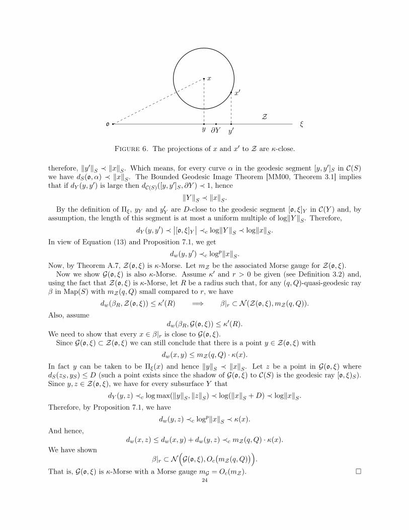
o ξZ

x

x′

y ∂Y y′

Figure 6. The projections of x and x′ to Z are κ-close.

therefore, ‖y′‖S ≺ ‖x‖S . Which means, for every curve α in the geodesic segment [y, y′]S in C(S)we have dS(o, α) ≺ ‖x‖S . The Bounded Geodesic Image Theorem [MM00, Theorem 3.1] impliesthat if dY (y, y′) is large then dC(S)([y, y′]S , ∂Y ) ≺ 1, hence

‖Y ‖S ≺ ‖x‖S .By the definition of Πξ, yY and y′Y are D-close to the geodesic segment [o, ξ]Y in C(Y ) and, by

assumption, the length of this segment is at most a uniform multiple of log‖Y ‖S . Therefore,dY (y, y′) ≺

∣∣[o, ξ]Y ∣∣ ≺c log‖Y ‖S ≺ log‖x‖S .In view of Equation (13) and Proposition 7.1, we get

dw(y, y′) ≺c logp‖x‖S .Now, by Theorem A.7, Z(o, ξ) is κ-Morse. Let mZ be the associated Morse gauge for Z(o, ξ).

Now we show G(o, ξ) is also κ-Morse. Assume κ′ and r > 0 be given (see Definition 3.2) and,using the fact that Z(o, ξ) is κ-Morse, let R be a radius such that, for any (q,Q)-quasi-geodesic rayβ in Map(S) with mZ(q,Q) small compared to r, we have

dw(βR,Z(o, ξ)) ≤ κ′(R) =⇒ β|r ⊂ N (Z(o, ξ),mZ(q,Q)).

Also, assumedw(βR,G(o, ξ)) ≤ κ′(R).

We need to show that every x ∈ β|r is close to G(o, ξ).Since G(o, ξ) ⊂ Z(o, ξ) we can still conclude that there is a point y ∈ Z(o, ξ) with

dw(x, y) ≤ mZ(q,Q) · κ(x).

In fact y can be taken to be Πξ(x) and hence ‖y‖S ≺ ‖x‖S . Let z be a point in G(o, ξ) wheredS(zS , yS) ≤ D (such a point exists since the shadow of G(o, ξ) to C(S) is the geodesic ray [o, ξ)S).Since y, z ∈ Z(o, ξ), we have for every subsurface Y that

dY (y, z) ≺c log max(‖y‖S , ‖z‖S) ≺ log(‖x‖S +D) ≺ log‖x‖S .Therefore, by Proposition 7.1, we have

dw(y, z) ≺c logp‖x‖S ≺ κ(x).

And hence,dw(x, z) ≤ dw(x, y) + dw(y, z) ≺c mZ(q,Q) · κ(x).

We have shownβ|r ⊂ N

(G(o, ξ), Oc

(mZ(q,Q)

)).

That is, G(o, ξ) is κ-Morse with a Morse gauge mG = Oc(mZ). 24

7.2. Convergence to the κ-Morse boundary. Let µ be a probability measure on Map(S). Wesay that µ is non-elementary if the semigroup generated by its support contains two pseudo-Anosovelements with disjoint fixed sets in PMF .

Let us recall some useful facts on random walks on the mapping class group.

Theorem 7.8. Let µ be a finitely supported, non-elementary probability measure on Map(S). Then:(1) For almost every sample path ω = (wn), the sequence (wn) converges to a point ξω in the

Gromov boundary of C(S), which is EL(S).(2) Moreover, there exists ` > 0, c < 1 such that

P (dS(o, wn) ≥ `n) ≥ 1− cn

for any n.(3) Further, for any k > 0 there exists C > 0 such that

P (dS(wn, γω) ≥ C log n) ≤ n−k

for any n, where γω = [o, ξω)S.

Claim (2) is proven by Maher ([Mah10], [Mah12]), while (1) and (3) are proven in [MT18]. Also,exactly the same proof as in [QRT19, Theorem A.17] (inspired by [ST19] and [Sis17, Lemma 4.4]),yields for the mapping class group:

Theorem 7.9. Let µ be a finitely supported, non-elementary probability measure on Map(S). Thenfor any k > 0 there exists C > 0 such that for all n we have

P(

supYdY (o, wn) ≥ C log n

)≤ Cn−k,

where the supremum is taken over all (proper) subsurfaces Y of S. As a consequence, for almostevery sample path there exists C > 0 such that for all n

supYdY (o, wn) ≤ C log n.

We now prove show that almost every sample path converges to a point in the κ-Morse boundaryof the mapping class group, where κ(r) = logp(r).

Theorem 7.10. Let µ be a finitely supported, non-elementary probability measure on Map(S), andlet κ(r) := logp(r). Then:

(1) Almost every sample path ω = (wn) converges to a point in the κ-Morse boundary withrespect to the topology of X ∪ ∂κX;

(2) Moreover, for almost every sample path there exists a κ-Morse geodesic ray Gω in Map(S)such that

lim supn→∞

d(wn,Gω)

logp+1(n)< +∞.

Proof. By Theorem 7.8, for almost every sample path, wnθ converges to a point ξω on the boundaryof C(S) (with respect to the topology on C(S) ∪ EL(S)).

Let G = G(o, ξω) be a resolution of a hierarchy towards ξω and let γω := [o, ξω)S be the shadowof G, which is a geodesic ray in C(S) starting from θ and limiting to ξω.

By Proposition 7.7, in order to prove that G is κ-Morse, it is sufficient to prove that there is aconstant c such that

(14) supYdY (o, ξω) ≤ c log dS(o, ∂Y ).

In the next few steps, we will show that (14) holds for almost every ω.25

Let pn be a nearest point projection (in C(S)) of wnθ to γω and cn := ctr(o, wn, ξω). By thedefinition of center and the hyperbolicity of C(S), there is D′ > 0 depending on D and δ such thatdS(cn, pn) ≤ D′ for any n.

Step 1. We claim that there exists C > 0 such that

(15) P(supYdY (wn, cn) ≥ C log n) ≤ Cn−2

for all n.

Proof. Since the drift of the random walk is positive with exponential decay (Theorem 7.8 (2)), wehave by the Markov property that there exists 0 < C0 < 1 such that

(16) P(dS(wn, w2n) ≤ `n) = P(dS(o, wn) ≤ `n) ≤ (C0)n ∀n

where ` > 0 is the drift of the random walk. By Theorem 7.8 (3), there exists C1 > 0 so that

(17) P(dS(wn, pn) ≥ C1 log n) ≤ C1n−2 ∀n

and, by Theorem 7.9, there exists C2 > 0 such that

(18) P(supYdY (wn, w2n) ≥ C2 log n) = P(sup

YdY (o, wn) ≥ C2 log n) ≤ C2n

−2 ∀n.

Now, since projection in a δ-hyperbolic space is coarsely distance-decreasing,

dY (wn, w2n) ≤ C2 log n

impliesdY (cn, c2n) ≤ C2 log n+ 2D,

for some D which depends only on δ, hence we also have for some new constant C3 > 0

(19) P(supYdY (cn, c2n) ≥ C3 log n) ≤ C3n

−2 ∀n.

Now, the complement of the union of all events expressed by (16), (17),(18),(19) has measure atleast 1− C5n

−2 for some new C5. We will consider from now on a sample path in such a set.Let us now pick a subsurface Y . By the bounded geodesic image theorem, there exists C4

(independent of Y ) such that if ∂Y is far from the geodesic segment [wn, pn] in C(S), namely

dC(S)(∂Y, [wn, pn]) ≥ C4,

then dY (wn, cn) ≤ C4 is uniformly bounded.On the other hand, if dC(S)(∂Y, [wn, pn]) ≤ C4, let us denote by q1 a nearest point projection of

∂Y onto [wn, pn] and by q2 a nearest point projection of ∂Y onto [w2n, p2n]. Then

dS(∂Y, [w2n, p2n]) = dS(∂Y, q2) ≥ dS(wn, w2n)− dS(∂Y, q1)− dS(q1, wn)− dS(w2n, q2)

≥ dS(wn, w2n)− dS(∂Y, q1)− dS(wn, pn)− dS(w2n, p2n)

≥ `n− C4 − C1 log n− C1 log(2n) > C4

for n sufficiently large (independently of Y and ω). Hence, by the bounded geodesic image theorem,

dY (w2n, c2n) ≤ C4.

By putting these estimates together and by the triangle inequality we obtain

dY (wn, cn) ≤ dY (wn, w2n) + dY (w2n, c2n) + dY (c2n, cn)

≤ C2 log n+ C4 + C3 log n ≤ C log n

by setting C appropriately, which proves the claim. 26

Step 2. We show that there exists a constant C7 such that for any n we have

(20) P(supYdY (o, cn) ≥ C7 log dS(o, pn) + C7) ≤ C7n

−2.

Proof. First note that by the triangle inequality if dS(o, wn) ≥ `n and dS(wn, pn) ≤ C1 log n then

dS(o, pn) ≥ dS(o, wn)− dS(wn, pn)

≥ `n− C1 log n ≥ `n/2

for n sufficiently large, hence by (16) and (17) there exists C6 for which

P(dS(o, pn) ≥ `n/2) ≥ 1− C6n−2 ∀n.

Then, by the triangle inequality

dY (o, cn) ≤ dY (o, wn) + dY (wn, cn)

and by Theorem 7.9 and Step 1.

≤ C2 log n+ C log n

≤ (C2 + C) log dS(o, pn) + (C2 + C) log(2/`)

≤ C7 log dS(o, pn) + C7

for the appropriate choice of C7.

Step 3. For almost every ω, there exists C8(ω) such that,

(21) dY (o, ξω) ≤ C8(ω) log dS(o, ∂Y )

for every subsurface Y 6= S.

Proof. By Step 2. and Borel-Cantelli, for almost every ω there exists n0 = n0(ω) such that

(22) supYdY (o, cn) ≤ C7 log dS(o, pn) + C7

for any n ≥ n0.Now, observe that the random walk is finitely supported, so dS(wn, wn+1) is uniformly bounded,

hence, since nearest point projection is coarsely distance decreasing, there exists D1 > 0 such that

dS(pn, pn+1) ≤ D1

is also uniformly bounded.Now, let Y be a subsurface. By the bounded geodesic image theorem, dY (o, ξω) ≤ C4 unless ∂Y

lies in a C4-neighborhood of [o, ξω)S . Let us suppose that ∂Y lies in a C4-neighborhood of [o, ξω)Sand let n = n(Y, ω) be the smallest integer such that dS(o, pn) ≥ dS(o, ∂Y ) + C4.

Note that by minimality, dS(o, pn) − D1 ≤ dS(o, pn−1) ≤ dS(o, ∂Y ) + C4 ≤ dS(o, pn), hencedS(o, pn) ≤ dS(o, ∂Y ) +D1 + C4.

Moreover, by the bounded geodesic image theorem,

|dY (o, ξω)− dY (o, cn)| ≤ C4

since the projection of [pn, ξ)S to C(Y ) is uniformly bounded. Hence by (22), if n ≥ n0(ω) then

dY (o, ξω) ≤ dY (o, cn) + C4

≤ C7 log dS(o, pn) + C7 + C4

≤ C7 log(dS(o, ∂Y ) +D1 + C4) + C7 + C4

27

On the other hand, if n(Y, ω) ≤ n0(ω) then dS(o, ∂Y ) ≤ dS(o, pn) ≤ dS(o, pn0(ω)), and there are atmost finitely many such subsurfaces Y for which the projection of [o, ξω)S onto C(Y ) is large. Hence

supY :n(Y,ω)≤n0

dY (o, ξω) < +∞,

thus the claim follows by adjusting the constant to a constant C8(ω), which depends on ω, to takeinto account the initial part.

Now, from (14) and Proposition 7.7, we obtain that the quasi-geodesic ray G in Map(S) is κ-Morse.

Let us now prove the second claim, namely the tracking estimate between the sample path andthe geodesic ray. From that and Lemma 4.3, it follows that almost every sample path converges inthe topology of X ∪ ∂κX.

For a given sample path ω = (wn), let ξ ∈ EL(S) be the ending lamination the path (wn) isconverging to, and let cn := ctr(o, wn, ξ). Note that by construction the projection of cn onto C(S)is within uniformly bounded distance of pn. Then, by equation (15), there exists C > 0 such that

P(supYdY (wn, cn) ≥ C log n) ≤ Cn−2

for any n. Applying Proposition 7.1 with D = log n, there exists C > 0 such that

(23) P(dw(wn, cn) ≥ C logp+1(n)) ≤ Cn−2

for any n. As a consequence, the Borel-Cantelli lemma implies that for almost every ω ∈ Ω thereexists n0 such that

(24) dw(wn, cn) ≤ C logp+1(n)

for all n ≥ n0. The claim follows by noting that dw(wn,G) ≤ dw(wn, cn) +O(1).

We now complete the proof of Theorem C by identifying the κ-Morse boundary with the Poissonboundary.

Theorem 7.11. Let µ be a non-elementary, finitely supported measure on G = Map(S). Then forκ(r) := logp(r), the κ-Morse boundary is a model for the Poisson boundary of (G,µ).

Proof. By Theorem 7.10, almost every sample path sublinearly tracks a κ-Morse geodesic ray, withκ(r) = logp(r), so we can apply Theorem 6.2.

8. Relatively hyperbolic groups

8.1. Background. Let G be a finitely generated group, and let P1, P2, . . . , Pk be a set of subgroupsof G which we call peripheral subgroups. Fix a finite generating set S. Let (G, dG) denote the Cayleygraph ofG with respect to S, equipped with the word metric. Following [Sis13], we denote by (G, d

G)

the metric graph obtained from the Cayley graph of G by adding an edge between every pair ofdistinct vertices contained in a left coset P of a peripheral subgroup. Setting up this way, G andG have the same vertex set, so any set in G can also be considered as a set in G. However, forx, y ∈ G, d

G(x, y) ≤ dG(x, y). In this Section, [x, y] will denote the geodesic segment between x, y

in the metric dGand Jx, yK the geodesic segment in dG.

Definition 8.1. A group G is relatively hyperbolic, relative to peripheral subgroups P1, P2, . . . , Pk,if the graph G has the properties:

• It is δ-hyperbolic;• It is fine: for each integer n, every edge belongs to only finitely many simple cycles of lengthn.

28

The collection of all cosets of peripheral subgroups is denoted by P. We shall denote as ND(P ) theD-neighborhood of P in the metric dG.

Moreover, we say a relatively hyperbolic group is non-elementary if it is infinite, not virtuallycyclic, and each Pi is infinite and with infinite index in G. We now fix a non-elementary relativelyhyperbolic group G and a generating set. We shall use the symbols ≺ and as before, wherethe implicit constants depend only on G and the generating set; we shall write K if the implicitconstants additionally depend on K. By definition of relative hyperbolicity, the graph G is δ-hyperbolic for some δ > 0. Moreover, for P ∈ P we let πP : G → P be a nearest point projectionto P , and denote

dP (x, y) := dG(πP (x), πP (y)).

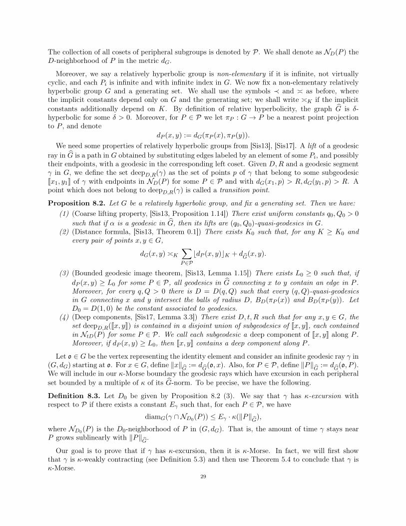
We need some properties of relatively hyperbolic groups from [Sis13], [Sis17]. A lift of a geodesicray in G is a path in G obtained by substituting edges labeled by an element of some Pi, and possiblytheir endpoints, with a geodesic in the corresponding left coset. Given D,R and a geodesic segmentγ in G, we define the set deepD,R(γ) as the set of points p of γ that belong to some subgeodesicJx1, y1K of γ with endpoints in ND(P ) for some P ∈ P and with dG(x1, p) > R, dG(y1, p) > R. Apoint which does not belong to deepD,R(γ) is called a transition point.

Proposition 8.2. Let G be a relatively hyperbolic group, and fix a generating set. Then we have:(1) (Coarse lifting property, [Sis13, Proposition 1.14]) There exist uniform constants q0, Q0 > 0

such that if α is a geodesic in G, then its lifts are (q0, Q0)-quasi-geodesics in G.(2) (Distance formula, [Sis13, Theorem 0.1]) There exists K0 such that, for any K ≥ K0 and

every pair of points x, y ∈ G,

dG(x, y) K∑P∈PbdP (x, y)cK + d

G(x, y).

(3) (Bounded geodesic image theorem, [Sis13, Lemma 1.15]) There exists L0 ≥ 0 such that, ifdP (x, y) ≥ L0 for some P ∈ P, all geodesics in G connecting x to y contain an edge in P .Moreover, for every q,Q > 0 there is D = D(q,Q) such that every (q,Q)-quasi-geodesicsin G connecting x and y intersect the balls of radius D, BD(πP (x)) and BD(πP (y)). LetD0 = D(1, 0) be the constant associated to geodesics.

(4) (Deep components, [Sis17, Lemma 3.3]) There exist D, t,R such that for any x, y ∈ G, theset deepD,R(Jx, yK) is contained in a disjoint union of subgeodesics of Jx, yK, each containedin NtD(P ) for some P ∈ P. We call each subgeodesic a deep component of Jx, yK along P .Moreover, if dP (x, y) ≥ L0, then Jx, yK contains a deep component along P .

Let o ∈ G be the vertex representing the identity element and consider an infinite geodesic ray γ in(G, dG) starting at o. For x ∈ G, define ‖x‖

G:= d

G(o, x). Also, for P ∈ P, define ‖P‖

G:= d

G(o, P ).

We will include in our κ-Morse boundary the geodesic rays which have excursion in each peripheralset bounded by a multiple of κ of its G-norm. To be precise, we have the following.

Definition 8.3. Let D0 be given by Proposition 8.2 (3). We say that γ has κ-excursion withrespect to P if there exists a constant Eγ such that, for each P ∈ P, we have

diamG(γ ∩ND0(P )) ≤ Eγ · κ(‖P‖G

),

where ND0(P ) is the D0-neighborhood of P in (G, dG). That is, the amount of time γ stays nearP grows sublinearly with ‖P‖

G.

Our goal is to prove that if γ has κ-excursion, then it is κ-Morse. In fact, we will first showthat γ is κ-weakly contracting (see Definition 5.3) and then use Theorem 5.4 to conclude that γ isκ-Morse.

29

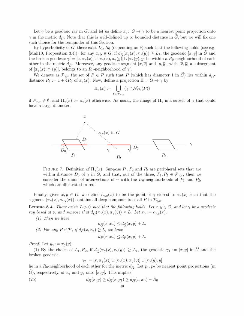
Let γ be a geodesic ray in G, and let us define πγ : G→ γ to be a nearest point projection ontoγ in the metric d

G. Note that this is well-defined up to bounded distance in G, but we will fix one

such choice for the remainder of this Section.By hyperbolicity of G, there exist L1, R0 (depending on δ) such that the following holds (see e.g.

[Mah10, Proposition 3.4]): for any x, y ∈ G, if dG

(πγ(x), πγ(y)) ≥ L1, the geodesic [x, y] in G andthe broken geodesic γ′ = [x, πγ(x)]∪ [πγ(x), πγ(y)]∪ [πγ(y), y] lie within a R0-neighborhood of eachother in the metric d

G. Moreover, any geodesic segment [x, x] and [y, y], with [x, y] a subsegment

of [πγ(x), πγ(y)], belongs to an R0-neighborhood of γ′.We denote as Pγ,x the set of P ∈ P such that P (which has diameter 1 in G) lies within d

G-

distance R1 := 1 + 4R0 of πγ(x). Now, define a projection Πγ : G→ γ by

Πγ(x) :=⋃

P∈Pγ,x

(γ ∩ND0(P ))

if Pγ,x 6= ∅, and Πγ(x) := πγ(x) otherwise. As usual, the image of Πγ is a subset of γ that couldhave a large diameter.

γD0

D0

D0

πγ(x) in G

P1 P2P3

x

Figure 7. Definition of Πγ(x). Suppose P1, P2 and P3 are peripheral sets that arewithin distance D0 of γ in G, and that, out of the three, P1, P2 ∈ Pγ,x; then weconsider the union of intersections of γ with the D0-neighborhoods of P1 and P2,which are illustrated in red.

Finally, given x, y ∈ G, we define cγ,y(x) to be the point of γ closest to πγ(x) such that thesegment Jπγ(x), cγ,y(x)K contains all deep components of all P in Pγ,x.Lemma 8.4. There exists L > 0 such that the following holds. Let x, y ∈ G, and let γ be a geodesicray based at o, and suppose that d

G(πγ(x), πγ(y)) ≥ L. Let xγ := cγ,y(x).

(1) Then we havedG

(x, xγ) ≤ dG

(x, y) + L.

(2) For any P ∈ P, if dP (x, xγ) ≥ L, we have

dP (x, xγ) ≤ dP (x, y) + L.

Proof. Let yγ := πγ(y).(1) By the choice of L1, R0, if dG(πγ(x), πγ(y)) ≥ L1, the geodesic γ1 := [x, y] in G and the

broken geodesicγ2 := [x, πγ(x)] ∪ [πγ(x), πγ(y)] ∪ [πγ(y), y]

lie in a R0-neighborhood of each other for the metric dG. Let p1, p2 be nearest point projections (in

G), respectively, of xγ and yγ onto [x, y]. This implies

dG

(x, y) ≥ dG

(x, p1) ≥ dG(x, xγ)−R0(25)30

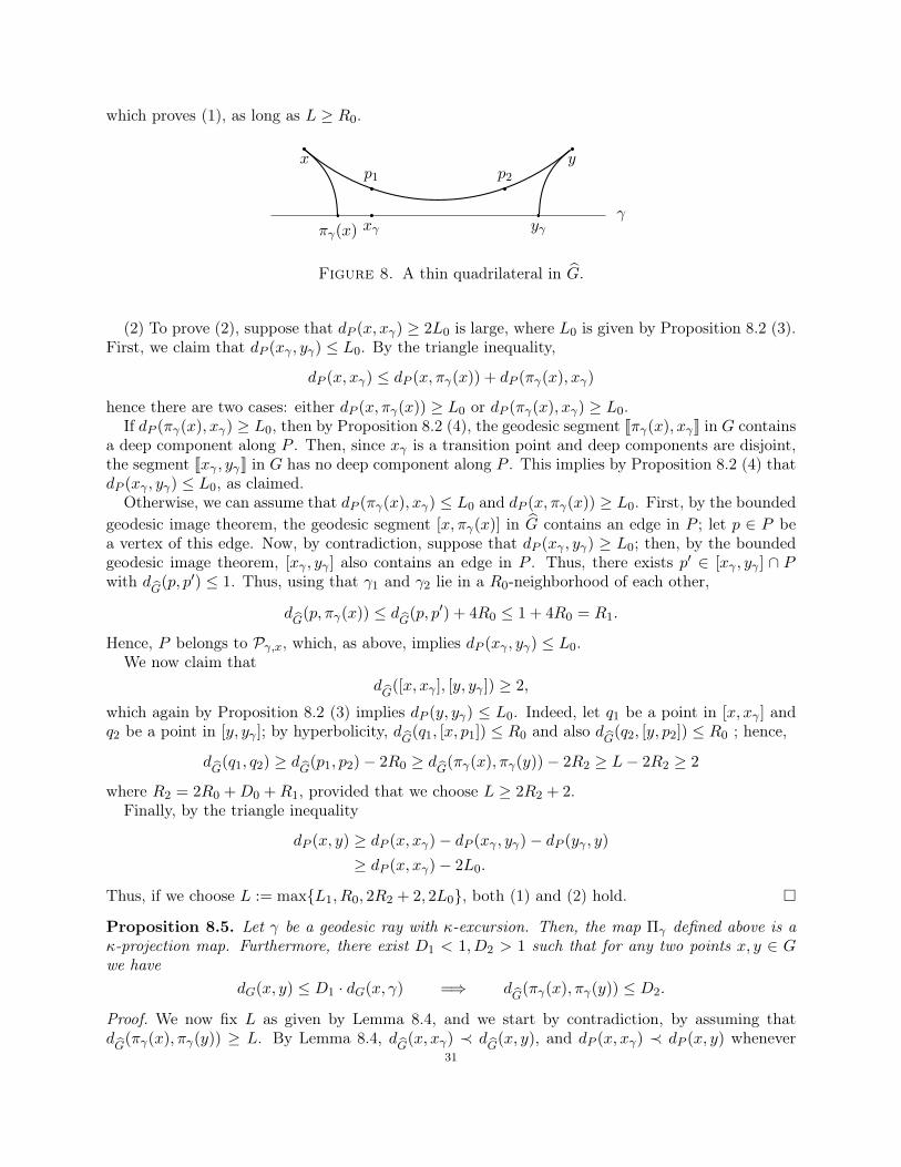
which proves (1), as long as L ≥ R0.

πγ(x) yγ

x y

xγ

p1 p2

γ

Figure 8. A thin quadrilateral in G.

(2) To prove (2), suppose that dP (x, xγ) ≥ 2L0 is large, where L0 is given by Proposition 8.2 (3).First, we claim that dP (xγ , yγ) ≤ L0. By the triangle inequality,

dP (x, xγ) ≤ dP (x, πγ(x)) + dP (πγ(x), xγ)

hence there are two cases: either dP (x, πγ(x)) ≥ L0 or dP (πγ(x), xγ) ≥ L0.If dP (πγ(x), xγ) ≥ L0, then by Proposition 8.2 (4), the geodesic segment Jπγ(x), xγK in G contains

a deep component along P . Then, since xγ is a transition point and deep components are disjoint,the segment Jxγ , yγK in G has no deep component along P . This implies by Proposition 8.2 (4) thatdP (xγ , yγ) ≤ L0, as claimed.

Otherwise, we can assume that dP (πγ(x), xγ) ≤ L0 and dP (x, πγ(x)) ≥ L0. First, by the boundedgeodesic image theorem, the geodesic segment [x, πγ(x)] in G contains an edge in P ; let p ∈ P bea vertex of this edge. Now, by contradiction, suppose that dP (xγ , yγ) ≥ L0; then, by the boundedgeodesic image theorem, [xγ , yγ ] also contains an edge in P . Thus, there exists p′ ∈ [xγ , yγ ] ∩ Pwith d

G(p, p′) ≤ 1. Thus, using that γ1 and γ2 lie in a R0-neighborhood of each other,

dG

(p, πγ(x)) ≤ dG

(p, p′) + 4R0 ≤ 1 + 4R0 = R1.

Hence, P belongs to Pγ,x, which, as above, implies dP (xγ , yγ) ≤ L0.We now claim that

dG

([x, xγ ], [y, yγ ]) ≥ 2,

which again by Proposition 8.2 (3) implies dP (y, yγ) ≤ L0. Indeed, let q1 be a point in [x, xγ ] andq2 be a point in [y, yγ ]; by hyperbolicity, d

G(q1, [x, p1]) ≤ R0 and also d

G(q2, [y, p2]) ≤ R0 ; hence,

dG

(q1, q2) ≥ dG(p1, p2)− 2R0 ≥ dG(πγ(x), πγ(y))− 2R2 ≥ L− 2R2 ≥ 2

where R2 = 2R0 +D0 +R1, provided that we choose L ≥ 2R2 + 2.Finally, by the triangle inequality

dP (x, y) ≥ dP (x, xγ)− dP (xγ , yγ)− dP (yγ , y)

≥ dP (x, xγ)− 2L0.

Thus, if we choose L := maxL1, R0, 2R2 + 2, 2L0, both (1) and (2) hold.

Proposition 8.5. Let γ be a geodesic ray with κ-excursion. Then, the map Πγ defined above is aκ-projection map. Furthermore, there exist D1 < 1, D2 > 1 such that for any two points x, y ∈ Gwe have

dG(x, y) ≤ D1 · dG(x, γ) =⇒ dG

(πγ(x), πγ(y)) ≤ D2.

Proof. We now fix L as given by Lemma 8.4, and we start by contradiction, by assuming thatdG

(πγ(x), πγ(y)) ≥ L. By Lemma 8.4, dG

(x, xγ) ≺ dG

(x, y), and dP (x, xγ) ≺ dP (x, y) whenever31

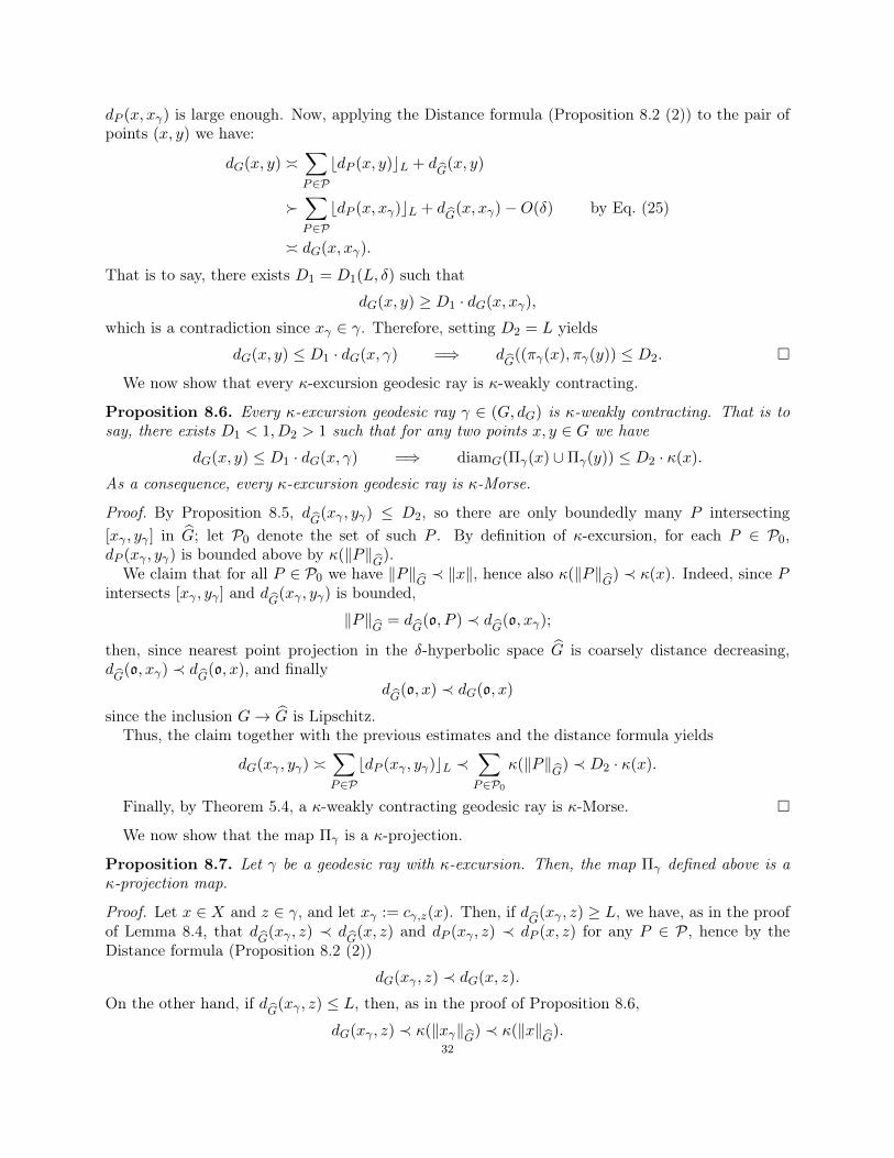
dP (x, xγ) is large enough. Now, applying the Distance formula (Proposition 8.2 (2)) to the pair ofpoints (x, y) we have:

dG(x, y) ∑P∈PbdP (x, y)cL + d

G(x, y)

∑P∈PbdP (x, xγ)cL + d

G(x, xγ)−O(δ) by Eq. (25)

dG(x, xγ).

That is to say, there exists D1 = D1(L, δ) such that

dG(x, y) ≥ D1 · dG(x, xγ),

which is a contradiction since xγ ∈ γ. Therefore, setting D2 = L yields

dG(x, y) ≤ D1 · dG(x, γ) =⇒ dG

((πγ(x), πγ(y)) ≤ D2.

We now show that every κ-excursion geodesic ray is κ-weakly contracting.

Proposition 8.6. Every κ-excursion geodesic ray γ ∈ (G, dG) is κ-weakly contracting. That is tosay, there exists D1 < 1, D2 > 1 such that for any two points x, y ∈ G we have

dG(x, y) ≤ D1 · dG(x, γ) =⇒ diamG(Πγ(x) ∪Πγ(y)) ≤ D2 · κ(x).

As a consequence, every κ-excursion geodesic ray is κ-Morse.

Proof. By Proposition 8.5, dG

(xγ , yγ) ≤ D2, so there are only boundedly many P intersecting[xγ , yγ ] in G; let P0 denote the set of such P . By definition of κ-excursion, for each P ∈ P0,dP (xγ , yγ) is bounded above by κ(‖P‖

G).

We claim that for all P ∈ P0 we have ‖P‖G≺ ‖x‖, hence also κ(‖P‖

G) ≺ κ(x). Indeed, since P

intersects [xγ , yγ ] and dG

(xγ , yγ) is bounded,

‖P‖G

= dG

(o, P ) ≺ dG

(o, xγ);

then, since nearest point projection in the δ-hyperbolic space G is coarsely distance decreasing,dG

(o, xγ) ≺ dG

(o, x), and finallydG

(o, x) ≺ dG(o, x)

since the inclusion G→ G is Lipschitz.Thus, the claim together with the previous estimates and the distance formula yields

dG(xγ , yγ) ∑P∈PbdP (xγ , yγ)cL ≺

∑P∈P0

κ(‖P‖G

) ≺ D2 · κ(x).

Finally, by Theorem 5.4, a κ-weakly contracting geodesic ray is κ-Morse.

We now show that the map Πγ is a κ-projection.

Proposition 8.7. Let γ be a geodesic ray with κ-excursion. Then, the map Πγ defined above is aκ-projection map.

Proof. Let x ∈ X and z ∈ γ, and let xγ := cγ,z(x). Then, if dG

(xγ , z) ≥ L, we have, as in the proofof Lemma 8.4, that d

G(xγ , z) ≺ d

G(x, z) and dP (xγ , z) ≺ dP (x, z) for any P ∈ P, hence by the

Distance formula (Proposition 8.2 (2))

dG(xγ , z) ≺ dG(x, z).

On the other hand, if dG

(xγ , z) ≤ L, then, as in the proof of Proposition 8.6,

dG(xγ , z) ≺ κ(‖xγ‖G) ≺ κ(‖x‖G

).32

Moreover, since γ has κ-excursion, we have diamG(Πγ(x)) ≺ Eγ · κ(‖xγ‖G) ≺ Eγ · κ(‖x‖G

). Thus,we obtain

diamG(Πγ(x) ∪ z) ≤ C1 · dG(x, z) + C2 · κ(x),

where C1, C2 depend only on γ, completing the proof.

The following is our main result on relatively hyperbolic groups.

Theorem 8.8. Let µ be a finitely supported probability measure on a relatively hyperbolic group G,and let S be a finite generating set. Let κ(r) := log r, and let ∂κX be the κ-Morse boundary of theCayley graph X of G with respect to S. Then:

(1) Almost every sample path (wn) converges to a point in ∂κX;(2) The pair (∂κX, ν), where ν is the hitting measure of the random walk on ∂κX, is a model

for the Poisson boundary of (G,µ).

Proof. The proof is fairly similar to the proof of Theorem 7.10 for the mapping class group, afterreplacing subsurfaces Y by peripherals P ∈ P, dY by dP , and the curve complex C(S) by G. Note,however, that one difference is that there need not be a hyperbolic space analogous to C(Y ) foreach P ∈ P; moreover, the concept of center is not well-defined. Essentially, the only step wherethe proof as written does not immediately generalize is the proof of Eq. (19), where we do notknow that nearest point projections are distance decreasing (not even coarsely). We shall give analternative proof of this point, not using the hyperbolicity of C(Y ).

By Theorem 7.8, almost every sample path ω = (wn) converges to a point ξω in the Gromovboundary of G. Consider a geodesic ray in G joining the base point o and ξω, and let γ = γω be alift to G.

Let cn := cγ,w2n(wn), following the notation before Lemma 8.4. We replace Step 1 in the proofof Theorem 7.10 with the following.

Step 1. We claim that there exists C > 0 such that

(26) P(supPdP (wn, cn) ≥ C log n) ≤ Cn−2

for all n.

Proof. Since the drift of the random walk is positive with exponential decay (Theorem 7.8 (2)), wehave by the Markov property that there exists 0 < C0 < 1 such that

(27) P(dG

(wn, w2n) ≤ `n) = P(dG

(o, wn) ≤ `n) ≤ (C0)n ∀n

where ` > 0 is the drift of the random walk. By Theorem 7.8 (3), and recalling that cn projectsclose to, there exists C1 > 0 so that

(28) P(dG

(wn, cn) ≥ C1 log n) ≤ C1n−2 ∀n.

If a sample path lies in the complement of the union of the events expressed by (27), (28), we have

dG

(cn, c2n) ≥ dG

(wn, w2n)− dG

(wn, cn)− dG

(w2n, c2n)

≥ `n− C1 log n− C2 log(2n) ≥ Lwhere L is given by Lemma 8.4, hence, by Lemma 8.4, we have

(29) dP (wn, cn) ≤ dP (wn, w2n) + L

for any P ∈ P. Moreover, by [Sis17, Lemma 4.4], there exists C2 > 0 for which

(30) P(supPdP (wn, w2n) ≥ C2 log n) = P(sup

PdY (o, wn) ≥ C2 log n) ≤ C2n

−2 ∀n.

hence, by combining Eq. (29) and (30) we obtain (26). 33

Then, we proceed exactly as in Theorem 7.10 (Steps 2 and 3), proving that for almost everyω ∈ Ω, there is a constant c such that

(31) supP∈P

diamG(γ ∩ND0(P )) ≤ c log dG

(o, P ).

Hence, by Proposition 8.6, the geodesic ray γω has κ-excursion, hence it is κ-Morse. This shows(1).

Finally, (2) follows by Theorem 6.1 using Theorem 6.2.

Remark 8.9. Continuing as in the proof of Theorem 7.10, the above argument also shows thefollowing tracking result: for almost every sample path there exists a geodesic ray γ in G such that

lim supn→∞

d(wn, γ)

log2(n)< +∞.

However, [Sis17] already shows the stronger tracking result with log(n) instead of log2(n), hence wedo not write out the details.

Appendix A. General projection and Weakly κ-Contracting Property

We begin this appendix by proving the following, announced in Section 5.

Theorem A.1 (κ-weakly contracting implies sublinearly Morse). Let κ be a concave sublinearfunction and let Z be a closed subspace of X. Let πZ be a κ-projection onto Z and suppose that Z isκ-weakly contracting with respect to πZ . Then, there is a function mZ : R2 → R such that, for everyconstant r > 0 and every sublinear function κ′, there is an R = R(Z, r, κ′) > 0 where the followingholds: Let η : [0,∞) → X be a (q,Q)-quasi-geodesic ray so that mZ(q,Q) is small compared to r,let tr be the first time ‖η(tr)‖ = r and let tR be the first time ‖η(tR)‖ = R. Then

dX(η(tR), Z

)≤ κ′(R) =⇒ η([0, tr]) ⊂ Nκ

(Z,mZ(q,Q)

).

Proof. Let C1, C2, D1, D2 be the constants which appear in the definitions of κ-projection and κ-weakly contracting (Definition 5.1 and Definition 5.3). Note that the condition of being κ-weaklycontracting becomes weaker as C1 gets smaller, hence we can assume that C1 ≤ 1/2. We first set

(32) m0 := max

q(qC2 + q + 1) +Q

C1,2C2(D1 + 1)

(q − 1), Q

, m1 := q(C2 + 1)(D1 + 1).

Claim A.2. Consider a time interval [s, s′] during which η is outside of Nκ(Z,m0). Then thereexists a constant A depending only on C1, C2, D1, D2, q,Q, such that

(33) |s′ − s| ≤ m1

(dX(η(s), Z

)+ dX

(η(s′), Z

))+ A · κ(η(s′)).

Proof of Claim A.2. Lets = t0 < t1 < t2 < · · · < t` = s′

be a sequence of times such that, for i = 0, . . . , `− 2, we have ti+1 is a first time after ti where

(34) dX(η(ti), η(ti+1)

)= C1dX(η(ti), Z) and dX

(η(t`−1), η(t`)

)≤ C1dX(η(t`−1), Z).

To simplify the notation, we define

ηi := η(ti), ri := ‖η(ti)‖and moreover, we pick some πi ∈ πZ(ηi) and let

dπi := dX(ηi, πi), di := dX(ηi, Z).

Note that, by assumption

(35) dπi ≥ di = dX(ηi, Z) ≥ m0 · κ(ri).34

Claim A.3. We have the inequality dπ`−1 ≤ 2(D1 + 1) dπ` +D2 · κ(η`−1).

Proof of Claim A.3. By the triangle inequality and Eq. (34),

dX(η`−1, Z) ≤ dX(η`−1, η`) + dX(η`, Z)

≤ C1dX(η`−1, Z) + dX(η`, Z)

hence, using C1 ≤ 1/2,

dX(η`−1, Z) ≤ 1

1− C1dX(η`, Z) ≤ 2dX(η`, Z).

Thus, by Lemma 5.2,

dπ`−1 ≤ (D1 + 1)dX(η`−1, Z) +D2 · κ(η`−1)

and by the above equation

≤ 2(D1 + 1)dX(η`, Z) +D2 · κ(η`−1)

≤ 2(D1 + 1)dπ` +D2 · κ(η`−1).

Now, since Z is κ-weakly contracting, by Definition 5.3 we get

dX(π0, π`

)≤

`−1∑i=0

dX(πi, πi+1

)≤

`−1∑i=0

C2 · κ(ri).

But η is (q,Q)-quasi-geodesic, hence,

|s′ − s| ≤ q dX(η0, η`) +Q

≤ q(dπ0 + dX

(π0, π`

)+ dπ`

)+Q(36)

≤ q C2

(`−1∑i=0

κ(ri)

)+ q (dπ0 + dπ` ) +Q.

On the other hand,

|s′ − s| =`−1∑i=0

|ti+1 − ti| ≥1

q

`−1∑i=0

(dX(ηi, ηi+1)−Q) .

Meanwhile, for i = 0, . . . , ` − 2 we have dX(ηi, ηi+1) = C1dX(ηi, Z). Furthermore, we have bytriangle inequality,

dX(η`−1, η`) + dπ` + dX(π`−1, π`) ≥ dπ`−1 ≥ dX(η`−1, Z),

which gives

dX(η`−1, η`) ≥ dX(η`−1, Z)− dπ` − C2 · κ(r`−1).35

Hence, together with Equation (35) and using C1 ≤ 1 we have

|s′ − s| ≥ 1

q

`−1∑i=0

(C1dX(ηi, Z)−Q)−dπ` + C2 · κ(r`−1)

q

≥ 1

q

`−1∑i=0

(C1m0 · κ(ri)−Q)−dπ`q− C2

κ(r`−1)

qBy Equation (35)

≥ 1

q

`−1∑i=0

(C1m0 · κ(ri)−Q · κ(ri))−dπ`q− C2

κ(r`−1)

qκ(t) ≥ 1 for all t

≥(C1m0 −Q

q

) `−1∑i=0

κ(ri)−dπ`q− C2

κ(r`−1)

q.

Combining the above inequality with Equation (36) we get

q (dπ0 + dπ` ) +Q+dπ`q

+ C2κ(r`−1)

q≥(C1m0 −Q

q− q C2

) `−1∑i=0

κ(ri)(37)

≥ (q + 1)`−1∑i=0

κ(ri),

where in the last step we plugged in the definition of m0 from (32).By (35) we also have

q (dπ0 + dπ` ) +Q+dπ`q

+ C2κ(r`−1)

q≤ q (dπ0 + dπ` ) +Q+

dπ`q

+ C2

dπ`−1m0 q

By the expression of m0 in (32), Q ≤ m0 and by Equation (35), m0 ≤ dπ0 . Thus we have Q ≤ dπ0and again by plugging in m0 and using Claim A.3, we obtain

q (dπ0 + dπ` ) +Q+dπ`q

+ C2

dπ`−1m0 q

≤ (q + 1)(dπ0 + dπ` ) +C2D2

m0 q· κ(η`−1).

Plugging this inequality into Equation (37), we get`−1∑i=0

κ(ri) ≤ dπ0 + dπ` +C2D2

m0 q(q + 1)· κ(η`−1)

≤ (D1 + 1)(d0 + d`) +D2(κ(η0) + κ(η`)) +C2D2

m0 q(q + 1)· κ(η`−1)

where we recall di = dX(ηi, Z), and the last inequality comes from Lemma 5.2 (note the differencebetween di and dπi = dX(ηi, πi)).

Lastly, we claim that since η is a quasi-geodesic ray, there is a constant C3, related to q,Q, suchthat ηi ≤ C3 · η(s′) +C3 for i = 0, . . . , `, hence also κ(ηi) ≤ 2C3 ·κ(η(s′)) +κ(2C3); thus, to shortenthe preceding expression, let A be a constant, depending on C1, C2, D1, D2, q,Q, κ, such that

q(C2 + 1)D2(κ(η0) + κ(η`)) +Q+C22D2

m0(q + 1)· κ(η`−1) ≤ A · κ(η(s′)).

By Equation (36) and the definition m1 = q(C2 + 1)(D1 + 1) from (32),

|s′ − s| ≤ m1(d0 + d`) + A · κ(η(s′)).

This proves Claim A.2. 36

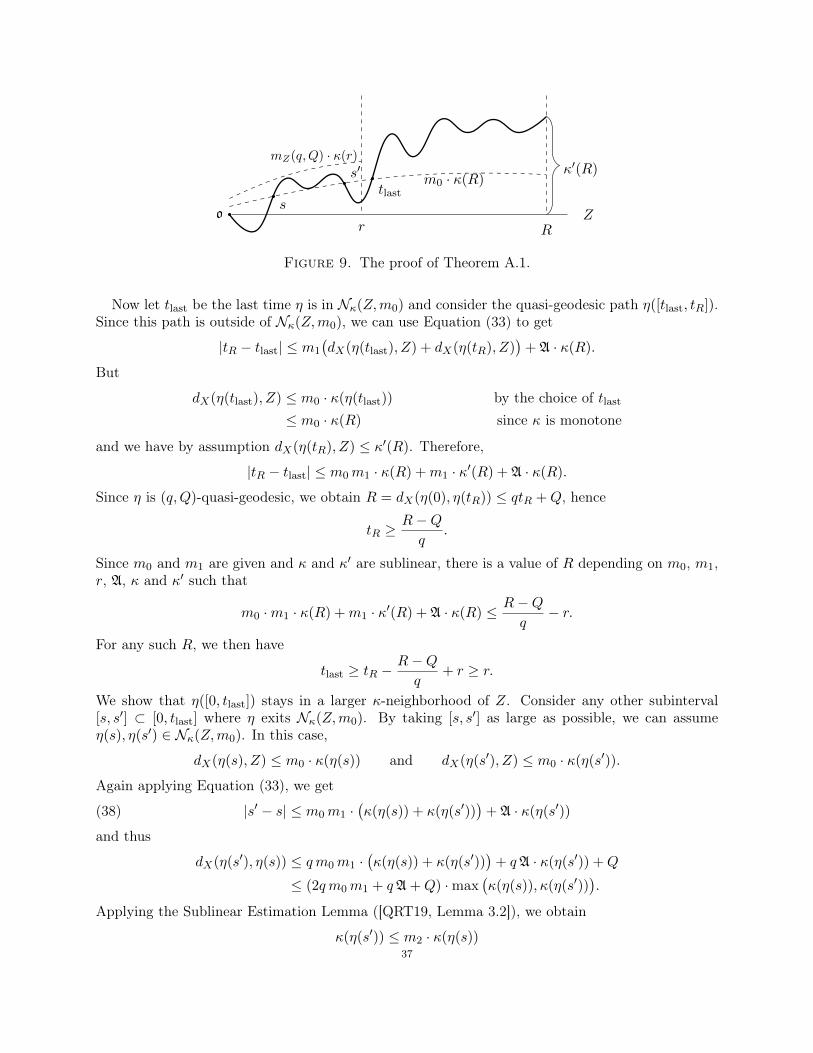
o Z

m0 · κ(R)

mZ(q,Q) · κ(r)

Rr

κ′(R)

tlasts

s′

Figure 9. The proof of Theorem A.1.

Now let tlast be the last time η is in Nκ(Z,m0) and consider the quasi-geodesic path η([tlast, tR]).Since this path is outside of Nκ(Z,m0), we can use Equation (33) to get

|tR − tlast| ≤ m1

(dX(η(tlast), Z) + dX(η(tR), Z)

)+ A · κ(R).

But

dX(η(tlast), Z) ≤ m0 · κ(η(tlast)) by the choice of tlast≤ m0 · κ(R) since κ is monotone

and we have by assumption dX(η(tR), Z) ≤ κ′(R). Therefore,

|tR − tlast| ≤ m0m1 · κ(R) +m1 · κ′(R) + A · κ(R).

Since η is (q,Q)-quasi-geodesic, we obtain R = dX(η(0), η(tR)) ≤ qtR +Q, hence

tR ≥R−Qq

.

Since m0 and m1 are given and κ and κ′ are sublinear, there is a value of R depending on m0, m1,r, A, κ and κ′ such that

m0 ·m1 · κ(R) +m1 · κ′(R) + A · κ(R) ≤ R−Qq− r.

For any such R, we then have

tlast ≥ tR −R−Qq

+ r ≥ r.

We show that η([0, tlast]) stays in a larger κ-neighborhood of Z. Consider any other subinterval[s, s′] ⊂ [0, tlast] where η exits Nκ(Z,m0). By taking [s, s′] as large as possible, we can assumeη(s), η(s′) ∈ Nκ(Z,m0). In this case,

dX(η(s), Z) ≤ m0 · κ(η(s)) and dX(η(s′), Z) ≤ m0 · κ(η(s′)).

Again applying Equation (33), we get

(38) |s′ − s| ≤ m0m1 ·(κ(η(s)) + κ(η(s′))

)+ A · κ(η(s′))

and thus

dX(η(s′), η(s)) ≤ q m0m1 ·(κ(η(s)) + κ(η(s′))

)+ qA · κ(η(s′)) +Q

≤ (2q m0m1 + qA +Q) ·max(κ(η(s)), κ(η(s′))

).

Applying the Sublinear Estimation Lemma ([QRT19, Lemma 3.2]), we obtain

κ(η(s′)) ≤ m2 · κ(η(s))37

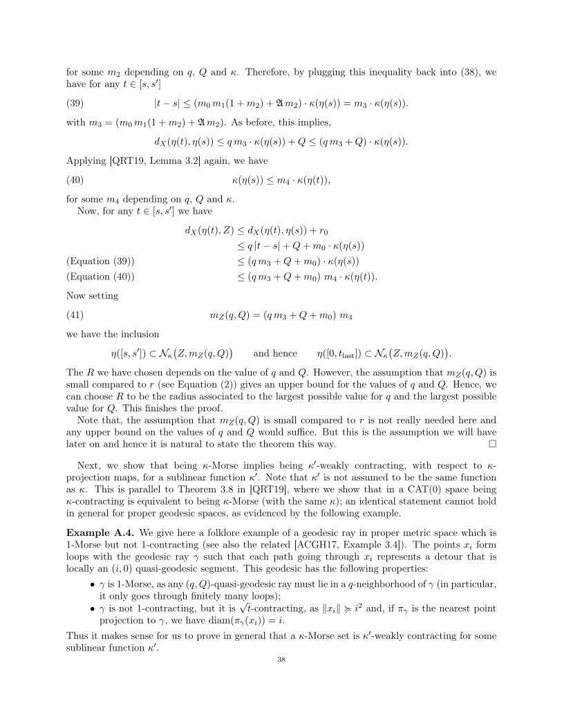
for some m2 depending on q, Q and κ. Therefore, by plugging this inequality back into (38), wehave for any t ∈ [s, s′]

(39) |t− s| ≤ (m0m1(1 +m2) + Am2) · κ(η(s)) = m3 · κ(η(s)).

with m3 = (m0m1(1 +m2) + Am2). As before, this implies,

dX(η(t), η(s)) ≤ q m3 · κ(η(s)) +Q ≤ (q m3 +Q) · κ(η(s)).

Applying [QRT19, Lemma 3.2] again, we have

(40) κ(η(s)) ≤ m4 · κ(η(t)),

for some m4 depending on q, Q and κ.Now, for any t ∈ [s, s′] we have

dX(η(t), Z) ≤ dX(η(t), η(s)) + r0

≤ q |t− s|+Q+m0 · κ(η(s))

≤ (q m3 +Q+m0) · κ(η(s))(Equation (39))≤ (q m3 +Q+m0) m4 · κ(η(t)).(Equation (40))

Now setting

(41) mZ(q,Q) = (q m3 +Q+m0) m4

we have the inclusion

η([s, s′]) ⊂ Nκ(Z,mZ(q,Q)

)and hence η([0, tlast]) ⊂ Nκ

(Z,mZ(q,Q)

).

The R we have chosen depends on the value of q and Q. However, the assumption that mZ(q,Q) issmall compared to r (see Equation (2)) gives an upper bound for the values of q and Q. Hence, wecan choose R to be the radius associated to the largest possible value for q and the largest possiblevalue for Q. This finishes the proof.

Note that, the assumption that mZ(q,Q) is small compared to r is not really needed here andany upper bound on the values of q and Q would suffice. But this is the assumption we will havelater on and hence it is natural to state the theorem this way.

Next, we show that being κ-Morse implies being κ′-weakly contracting, with respect to κ-projection maps, for a sublinear function κ′. Note that κ′ is not assumed to be the same functionas κ. This is parallel to Theorem 3.8 in [QRT19], where we show that in a CAT(0) space beingκ-contracting is equivalent to being κ-Morse (with the same κ); an identical statement cannot holdin general for proper geodesic spaces, as evidenced by the following example.

Example A.4. We give here a folklore example of a geodesic ray in proper metric space which is1-Morse but not 1-contracting (see also the related [ACGH17, Example 3.4]). The points xi formloops with the geodesic ray γ such that each path going through xi represents a detour that islocally an (i, 0) quasi-geodesic segment. This geodesic has the following properties:

• γ is 1-Morse, as any (q,Q)-quasi-geodesic ray must lie in a q-neighborhood of γ (in particular,it only goes through finitely many loops);• γ is not 1-contracting, but it is

√t-contracting, as ‖xi‖ < i2 and, if πγ is the nearest point

projection to γ, we have diam(πγ(xi)) = i.Thus it makes sense for us to prove in general that a κ-Morse set is κ′-weakly contracting for somesublinear function κ′.

38

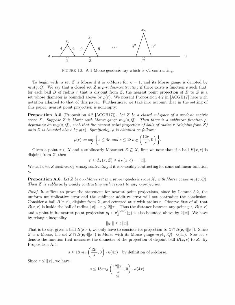
o γ

x2x3

xn

4 4 9 9n2 n2

2 3 n

Figure 10. A 1-Morse geodesic ray which is√t-contracting.

To begin with, a set Z is Morse if it is κ-Morse for κ = 1, and its Morse gauge is denoted bymZ(q,Q). We say that a closed set Z is ρ-radius-contracting if there exists a function ρ such that,for each ball B of radius r that is disjoint from Z, the nearest point projection of B to Z is aset whose diameter is bounded above by ρ(r). We present Proposition 4.2 in [ACGH17] here withnotation adapted to that of this paper. Furthermore, we take into account that in the setting ofthis paper, nearest point projection is nonempty:

Proposition A.5 (Proposition 4.2 [ACGH17]). Let Z be a closed subspace of a geodesic metricspace X. Suppose Z is Morse with Morse gauge mZ(q,Q). Then there is a sublinear function ρ,depending on mZ(q,Q), such that the nearest point projection of balls of radius r (disjoint from Z)onto Z is bounded above by ρ(r). Specifically, ρ is obtained as follows:

ρ(r) := sups

s ≤ 4r and s ≤ 18mZ

(12r

s, 0

).

Given a point x ∈ X and a sublinearly Morse set Z ⊆ X, first we note that if a ball B(x, r) isdisjoint from Z, then

r ≤ dX(x, Z) ≤ dX(x, o) = ‖x‖.We call a set Z sublinearly weakly contracting if it is κ-weakly contracting for some sublinear functionκ.

Proposition A.6. Let Z be a κ-Morse set in a proper geodesic space X, with Morse gaugemZ(q,Q).Then Z is sublinearly weakly contracting with respect to any κ-projection.

Proof. It suffices to prove the statement for nearest point projections, since by Lemma 5.2, theuniform multiplicative error and the sublinear additive error will not contradict the conclusion.Consider a ball B(x, r), disjoint from Z, and centered at x with radius r. Observe first of all thatB(x, r) is inside the ball of radius ‖x‖+ r ≤ 2‖x‖. Thus the distance between any point y ∈ B(x, r)

and a point in its nearest point projection y1 ∈ π(near)Z (y) is also bounded above by 2‖x‖. We haveby triangle inequality

‖y1‖ ≤ 4‖x‖.That is to say, given a ball B(x, r), we only have to consider its projection to Z ∩B(o, 4‖x‖). SinceZ is κ-Morse, the set Z ∩ B(o, 4‖x‖) is Morse with its Morse gauge mZ(q,Q) · κ(4x). Now let sdenote the function that measures the diameter of the projection of disjoint ball B(x, r) to Z. ByProposition A.5,

s ≤ 18mZ

(12r

s, 0

)· κ(4x) by definition of κ-Morse.

Since r ≤ ‖x‖, we have

s ≤ 18mZ

(12‖x‖s

, 0

)· κ(4x).

39

Suppose s is not a sublinear function of ‖x‖, that is to say, as ‖x‖ → ∞, there exists a sequence ofdisjoint balls Bi with projections si such that there exists a positive number c such that

limi→∞

si‖x‖i

≥ c

then for every ε, there exists N such that for all j > N ,

sj ≤ 18mZ

(12‖x‖jsj

, 0

)· κ(4xj)

≤ 18mZ

(12

(1

c− ε), 0

)· κ(4xj).

That is to say, s is bounded above by a sublinear function of ‖x‖, which means s itself is a sublinearfunction of ‖x‖, which is contrary to our assumption. Therefore, there does not exists such asequence of balls and thus s is a sublinear function of ‖x‖, which we denote as κ′(x).

Lastly, by Lemma 5.2, the same claim holds for all κ-projection maps.

To summarize, we prove the equivalence between κ-weakly contracting and κ-Morse (for a possiblydifferent κ) for any given closed set:

Theorem A.7. Let (X, o) be a proper geodesic metric space with a fixed base point. Let Z be aclosed set and π be a κ-projection in the sense of Definition 5.1. The following hold:

(1) If Z is κ-weakly contracting with respect to π, then it is κ-Morse;(2) If Z is κ-Morse, then it is κ′-weakly contracting with respect to π for some sublinear function

κ′.

Proof. If Z is κ weakly contracting, then by Theorem 5.3 it is κ-Morse. On the other hand, ifZ is κ-Morse, by Proposition A.6 there exists a sublinear function κ′ for which Z is κ′-weaklycontracting.

References

[AK11] Y. Algom-Kfir, Strongly contracting geodesics in outer space, Geom. Topol. 15 (2011), no. 4, 2181–2233.[ACGH17] G. Arzhantseva, C. Cashen, D. Gruber, and D. Hume, Characterizations of Morse quasi-geodesics via

superlinear divergence and sublinear contraction, Doc. Math. 22 (2017), 1193–1224.[ACT15] G. Arzhantseva, C. Cashen and J. Tao, Growth tight actions, Pacific J. Math. 278 (2015), no. 1, 1–49.[Beh06] J. Behrstock, Asymptotic geometry of the mapping class group and Teichmüller space, Geom. Topol. 10

(2006), 1523–1578.[BHS17] J. Behrstock, M. Hagen and A. Sisto, Hierarchically hyperbolic spaces, I: Curve complexes for cubical groups,

Geom. Topol. 21 (2017), no. 3, 1731–1804.[BF09] M. Bestvina and K. Fujiwara, A characterization of higher rank symmetric spaces via bounded cohomology,

Geom. Funct. Anal. 19 (2009), no. 1, 11–40.[Bou98] N. Bourbaki, General topology. Chapters 1-4, Translated from the French. Reprint of the 1989 English

translation. Elements of Mathematics (Berlin), Springer-Verlag, Berlin, 1998. vii+437.[Cas16] C. Cashen, Quasi-isometries need not induce homeomorphisms of contracting boundaries with the Gromov

product topology, Anal. Geom. Metr. Spaces 4 (2016), no. 1, 278–281.[CM19] C. Cashen and J. Mackay, A metrizable topology on the contracting boundary of a group, Trans. Amer.

Math. Soc. 372 (2019), no. 3, 1555–1600.[CS15] R. Charney and H. Sultan, Contracting boundaries of CAT(0) spaces, J. Topol. 8 (2015), no. 1, 93–117.[CD60] G. Choquet and J. Deny, Sur l’ équation de convolution µ = µ∗σ, C. R. Math. Acad. Sci. Paris 250 (1960),

799–801.[Cor18] M. Cordes, Morse boundaries of proper geodesic spaces, Groups Geom. Dyn. 11 (2017), no. 4, 1281–1306.[CDG20] M. Cordes, M. Dussaule, and I. Gekhtman, An embedding of the Morse boundary in the Martin boundary,

preprint arXiv:2004.14624.[CK00] C. B. Croke and B. Kleiner, Spaces with nonpositive curvature and their ideal boundaries, Topology 39

(2000), no. 3, 549–556.40

[Dru00] C. Drutu, Quasi-isometric classification of non-uniform latticed in semisimple groups of higher rank, Geom.Funct. Anal. 10 (2000), 327–388.

[DR09] M. Duchin and K. Rafi, Divergence of Geodesics in Teichmüller Space and the Mapping Class Group, Geom.Funct. Anal. 19 (2009), 722–742.

[DM60] E. B. Dynkin and M. B. Maljutov, Random walk on groups with a finite number of generators, Dokl. Akad.Nauk SSSR 137 (1961), 1042–1045.

[EFW12] A. Eskin, D. Fisher and K. Whyte, Coarse differentiation of quasi-isometries I: Spaces not quasi-isometricto Cayley graphs, Ann. of Math. (2) 176 (2012), no. 1, 221–260.

[EFW13] A. Eskin, D. Fisher and K. Whyte, Coarse differentiation of quasi-isometries II: Rigidity for Sol andlamplighter groups, Ann. of Math. (2) 177 (2013), no. 3, 869–910.

[EMR18] A. Eskin, H. Masur and K. Rafi, Rigidity of Teichmüller space, Geom. Topol. 22 (2018), no. 7, 4259–4306.[EMR17] A. Eskin, H. Masur and K. Rafi, Large scale rank of Teichmüller space, Duke Math. J. 166 (2017), no. 8,

1517–1572.[Far98] B. Farb, Relatively hyperbolic groups, Geom. Funct. Anal. 8 (1998), 810–840.[FM98] B. Farb and H. Masur, Superrigidity and mapping class groups, Topology 37 (1998), 1169–1176.[FT18] B. Forghani and G. Tiozzo, Shannon’s theorem for locally compact groups, preprint arXiv:1812.07292.[Fri37] A. Frink, Distance functions and the metrization problem, Bull. Amer. Math. Soc. 43 (1937), no. 2, 133–142.[Fur63] H. Furstenberg, A Poisson Formula for Semi-Simple Lie Groups, Ann. of Math. (2) 77 (1963), no. 2,

335–386.[GM12] F. Gautero and F. Mathéus, Poisson boundary of groups acting on R-trees, Israel J. Math. 191 (2012), no.

2, 585–646.[Gro87] M. Gromov, Hyperbolic groups, in S. Gersten (ed.), Essays in group theory, Mathematical Sciences Research

Institute Publications 8, Springer, New York, 1987, 75–263.[GQR] I. Gekhtman, Y. Qing and K. Rafi, QI-invariant model of Poisson boundaries of CAT(0) groups, in prepa-

ration.[Kai94] V. Kaimanovich, The Poisson boundary of hyperbolic groups, C. R. Acad. Sci. Paris 318 (1994), no. 1, 59–64.[Kai00] V. Kaimanovich, The Poisson formula for groups with hyperbolic properties, Ann. of Math. (2) 152 (2000),

no. 3, 659–692.[KM96] V. Kaimanovich and H. Masur, The Poisson boundary of the mapping class group, Invent. Math. 125 (1996),

no. 2, 221–264.[KM98] V. Kaimanovich and H. Masur, The Poisson boundary of Teichmüller space, J. Funct. Anal. 156 (1998),

no. 2, 301–332.[Kar11] A. Kar, Asymptotically CAT(0) groups, Publ. Mat. 55 (2011), no. 1, 67–91.[KM99] A. Karlsson and G. Margulis, A multiplicative ergodic theorem and nonpositively curved spaces, Comm.

Math. Phys. 208 (1999), no. 1, 107–123.[Kla98] E. Klarreich, The Boundary at Infinity of the Curve Complex and the Relative Teichmüller Space, preprint

arXiv:1803.10339.[Mah10] J. Maher, Linear progress in the complex of curves, Trans. Amer. Math. Soc. 362 (2010), no. 6, 2963–2991.[Mah12] J. Maher, Exponential decay in the mapping class group, J. Lond. Math. Soc. (2) 86 (2012), no. 2, 366–386.[MT18] J. Maher and G. Tiozzo, Random walks on weakly hyperbolic groups, J. Reine Angew. Math. 742, (2018),

187–239.[MM00] H. Masur and Y. Minsky, Geometry of the complex of curves. II. Hierarchical structure, Geom. Funct. Anal.

10 (2000), no. 4, 902–974.[Mor24] H. M. Morse, A fundamental class of geodesics on any closed surface of genus greater than one, Trans.

Amer. Math. Soc. 26 (1924), 25–60.[Qin16] Y. Qing, Geometry of Right-Angled Coxeter Groups on the Croke-Kleiner Spaces, Geom. Dedicata 183

(2016), no. 1, 113–122.[QRT19] Y. Qing, K. Rafi and G. Tiozzo, Sublinearly Morse boundary I: CAT(0) spaces, preprint arXiv:1909.02096[QT19] Y. Qing and G. Tiozzo, Excursions of generic geodesics in right-angled Artin groups and graph products,

Int. Math. Res. Not. IMRN (2019), rnz294.[RV18] K. Rafi and Y. Verberne, Geodesics in the mapping class groups, preprint arXiv:1810.12489.[Ser83] C. Series, Martin boundaries of random walks on Fuchsian groups, Israel J. Math. 44 (1983), 221–242.[Sis13] A. Sisto, Projections and relative hyperbolicity, Enseign. Math. (2) 59 (2013), no. 1-2, 165–181.[Sis17] A. Sisto, Tracking rates of random walks, Israel J. Math. 220 (2017), 1–28.[Sis18] A. Sisto, Contracting elements and random walks, J. Reine Angew. Math. 742 (2018), 79–114.[ST19] A. Sisto and S. Taylor, Largest projections for random walks and shortest curves for random mapping tori,

Math. Res. Lett. 26 (2019) no. 1, 293–321.

41

[Tio15] G. Tiozzo, Sublinear deviation between geodesics and sample paths, Duke Math. J. 164 (2015), no. 3, 511–539.

[Woe00] W. Woess, Random Walks on Infinite Graphs and Groups, Cambridge Tracts in Mathematics, CambridgeUniversity Press, Cambridge, 2000.

[Yan20] W. Yang, Genericity of contracting elements in groups, Math. Ann. 376 (2020), 823–861.

Department of Mathematics, Fudan University, ChinaE-mail address: yulan.qing@gmail.com

Department of Mathematics, University of Toronto, Toronto, ON, CanadaE-mail address: rafi@math.toronto.edu

Department of Mathematics, University of Toronto, Toronto, ON, CanadaE-mail address: tiozzo@math.toronto.edu

42