Vínculos internos y externos. Láminas y análisis de cadenas.
Dealing with Uncertaintiesin the Assessment of
Existing RC Buildings
Ludovica Elefante
Universityof NaplesFederico II
Ph.D. Programme in Engineering of Materials and Structures XXII cycle
Y
λY
P0P0
XYZ
Seismic Risk
Materials Defects
Structural Modeling Input
Knowledge Levels
123
0
UNIVERSITY OF NAPLES FEDERICO II Faculty of Engineering
PH.D. PROGRAMME in MATERIALS and STRUCTURES COORDINATOR PROF. DOMENICO ACIERNO
XXII CYCLE
LUDOVICA ELEFANTE
PH.D. THESIS
Dealing with Uncertainties in the Assessment of Existing RC Buildings
TUTOR PROF. ING. GAETANO MANFREDI CO-TUTOR DR. ING. IUNIO IERVOLINO,
DR. ING. FATEMEH JALAYER

II

III
“Anyone who has never made a mistake has never tried anything new”
Albert Einstein

IV

V
Acknowledgements I have decided to write these few words in Italian because it is the language of my feelings. Ad un passo dalla fine di questa meravigliosa esperienza ho la sensazione che questi tre anni siano passati troppo in fretta; probabilmente perché il Dipartimento di Ingegneria Strutturale è stato per me come una seconda “casa” e per questo desidero ringraziare l’intero dipartimento. Spero di essere in grado di esprimere la mia gratitudine ai professori Gaetano Manfredi e Edoardo Cosenza per le numerose opportunità di crescita intellettuale e umana che mi hanno offerto in questi anni; sentirmi parte della loro “squadra” è sempre stato per me motivo di orgoglio. Ringrazio Iunio Iervolino che mi ha accompagnato attraverso questa esperienza con impegno e pazienza; la sua passione e dedizione per la ricerca sono state in questi anni un esempio per me. Un ringraziamento speciale va a Fatemeh Jalayer; poter lavorare a suo fianco (anche in senso fisico per la posizione delle nostre scrivanie) mi ha arricchito profondamente, non solo da un punto di vista scientifico, ma anche personale ed umano. Vorrei inoltre ringraziare Andrea Prota, Gerardo Verderame e Marco Di Ludovico che fin dalla tesi di laurea hanno seguito il mio percorso sostenendomi e consigliandomi. Grazie a tutti i miei colleghi ed amici con i quali in questi anni ho condiviso difficoltà, scadenze, ma anche tanti momenti felici. Ringrazio di cuore tutta la mia famiglia che mi ha sempre sostenuto ed incoraggiato nei momenti difficili con infinita pazienza: devo a loro, ed in particolare ai miei genitori, ciò che sono. Grazie a Vitale che è la mia forza ed il mio conforto; credo che l’amore che ci lega mi renda ai suoi occhi migliore di quella che sono e ciò è per me uno stimolo continuo a migliorare.
Ludovica

VI

VII
Alla mia cara zia, Anna.

VIII
IX
Index
Introduction 1I.1. Objectives 2
I.2. Problems of Existing RC Buildings 4
I.3. Evolution of the Legislation and Practice Project 5
I.4. Evolution of Structural Materials 11
I.5. Open Issues in the Current Code-Based Approach 12
I.6. Variability in the Assessment Results 13
I.7. The Organization of the Thesis 14
I.8. References 17
Chapter I. Approaches to Structural Safety Problems 191. Introduction 192. Engineering Safety Problems 20
2.1. Deterministic Approach 202.2. Semi-Probabilistic Approach 202.3. Probabilistic Approach 21
2.3.1. Exact Probabilistic Approach 222.3.2. Simplified Probabilistic Approach 26
3. Aleatory and Epistemic Uncertainties 294. Statistical and Non-Statistical Information 29
X
5. Decision Making under Uncertainty 30 5.1. Bayesian Decision Theory 30 5.2. Classical Decision Theory 31
6. The Total Probability Theorem 32 7. Probabilistic Performance-Based Assessment 32
7.1. Decision Variables 32 7.2. Intensity Measures 33 7.3. Engineering Demand Parameter 33 7.4. Damage Measures 34 7.5. PBEE Probability Framework Equation 34
8. References 36
Chapter II. Confidence Factor: the State of Research 37 1. Some Interesting Works 37 2. Confidence Factor and Structural Reliability 38
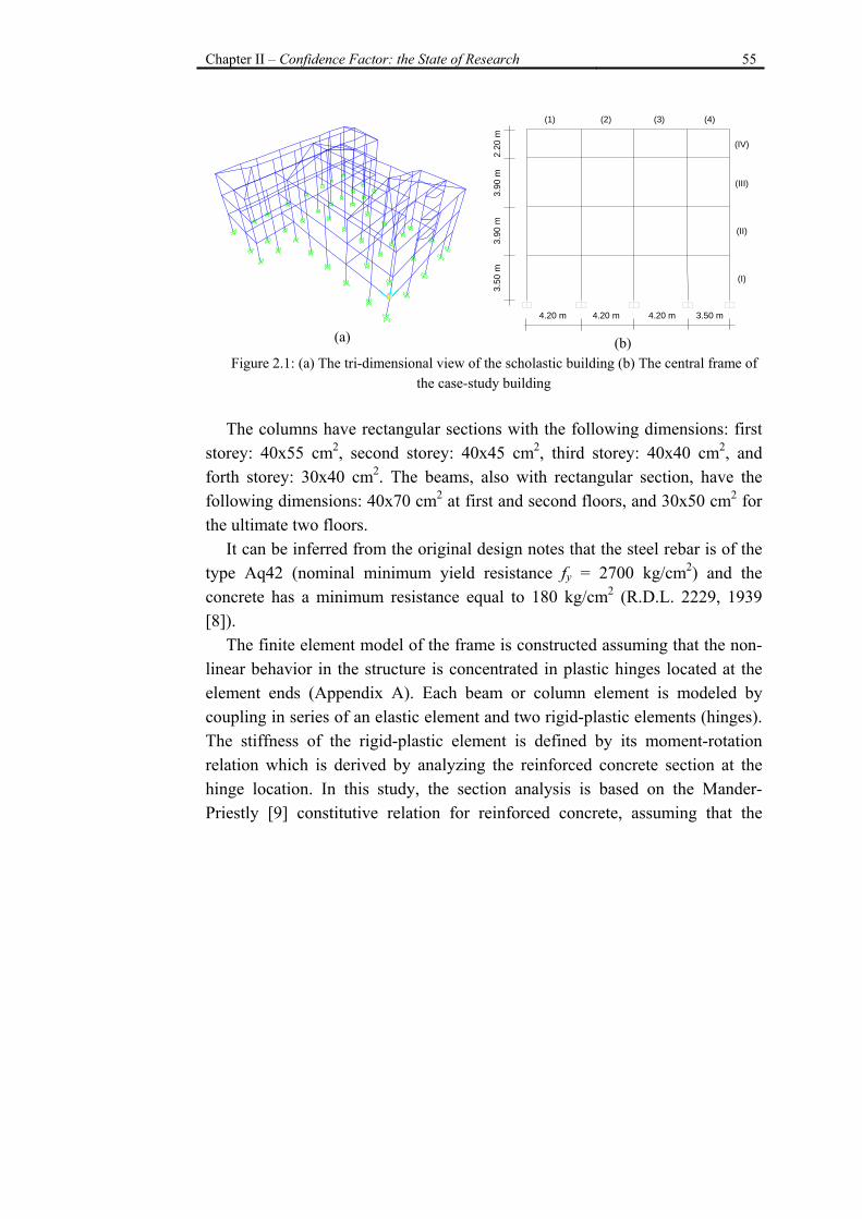
2.1. The Case-Study Structure 40 2.2. Evaluation of Robust Reliability 43 2.3. The Algorithm for Calculating the Structural Reliability 45 2.4. Calculating the Failure Probability using Subset Simulation 45 2.5. Structural Performance and Conventional Collapse 46 2.6. Characterization of Uncertainties 47
2.6.1. Materials 47 2.6.2. Structural Details 48
2.7. A Proposal for a Probabilistic Definition of Confidence Factors 49 3. Conclusions 51 4. References 53 Chapter III. Uncertainty in the Ground Motion Representation 55 1. Introduction 55 2. Ground Motion Record Selection 56
XI
3. Probabilistic Assessment based on Non-Linear Dynamic Analyis 573.1. The Intensity Measures for Predicting Structural Response 603.2. The Structural Engineering Parameter 61
4. The Case-Study Structure 625. The Suites of Ground Motion Records and Their Properties 63
5.1. Record Selection A 645.2. Record Selection B 65
6. The Disaggregation of Seismic Hazard 677. Residual-Residual Plot 718. The Cloud Method 74
8.1. The Weighted Cloud Method 759. The Multiple-Stripe Analysis 76
9.1. The Weighted Multiple-Stripe Analysis 779.2. Accounting for Collapse Cases in Multiple-Stripe Analysis 81
10. Numerical Results 8210.1. Cloud Method 82
10.1.1. Record Selection A 8310.1.2. Record Selection B 86
10.2. Multiple-Stripe Analysis 9210.2.1. Record Selection A 9310.2.2. Record Selection B 95
11. Conclusions 9812. References 103
Chapter IV. An Efficient Bayesian Method for Taking into Account the Modeling Uncertainties in the Evaluation of Structural Reliability 106
1. Introduction 1062. The Methodology 107
2.1. The Vector of Uncertain Parameters 107
XII
2.2. The Characterization of the Uncertainties 108 2.3. The Structural Performance Index 108 2.4. The Effect of Uncertainty on Structural Risk Assessment 109
3. A Closed-Form Solution for Structural Reliability 110 3.1. Uncertainty in Material Properties 111 3.2. Taking into Account Uncertainty in Structural Details 111 3.3. Taking into Account Uncertainty in Ground Motion
Representation 112 4. Numerical Results 115
4.1. The Structural Reliability given the Design Spectrum 115 4.2. The Structural Reliability taking into account Ground Motion
Uncertainty 118 5. Conclusions 121 6. References 123
Chapter V. An Alternative Performance-Based Safety-Checking Format 124
1. Introduction 124 2. The Knowledge Levels 125 3. The Methodology 126
3.1. Load and Resistance Factor Design Framework 126 3.2. Demand and Capacity Factor Design Framework 128
3.2.1. DCFD and PBEE Frameworks 129 3.2.2. Non-Linear Static Analysis 132 3.2.3. Non-Linear Dynamic Analysis 133
3.3. Characterization of the Uncertainties for KL0 134 3.3.1. Materials 135 3.3.2. Structural Details 135 3.3.3. Ground Motion 137
3.4. Updating the Probability Distributions 138
XIII
3.5. Using the Efficient Method for Estimating the Robust Reliability 142
4. Application to the Case-Study Structure 1464.1. Non-Linear Static Analysis 146
4.1.1. Calculation of the Structural Fragility 1464.1.2. Verification of Results Using the Standard Monte Carlo
Simulation 1514.2. Non-Linear Dynamic Analysis 152
4.2.1. The Code-Based Method 1534.2.2. Calculation of the Structural Reliability 155
5. Code-Based Implementation of the Alternative Performance-Based Safety-Checking Format 157
6. Conclusions 1597. References 163
Chapter VI. How to Characterize Prior Probability Distributions for Structural Details: a Survey for Professional Engineers 165
1. Introduction 1652. The Survey for Professional Engineers 1663. Preliminary Results 1804. References 184
Conclusions 185
Appendices 190A. Lumped Plasticity Model 190B. Plastic Hinge Characterization 193C. Capacity Spectrum Method 194D. Weighted Least Squares 198E. Shear Failure 200References 205

XIV
Introduction 15
Introduction
From a literature review it has been possible to point out, starting from Greek and Latin literature references, the development of at least 160 catastrophic seismic events in the Mediterranean.
Studies and researches have shown that about 60% of such events have been recorded in Italy as well as more than 50% of the recorded damages. This data can be ascribed to the high intensity of the recorded earthquakes in Italy, but also to both the high density of population and the presence of many structures under-designed or designed following old codes and construction practice: for this reasons the seismic risk in Italy is very high.
In fact, the seismic risk is defined by the convolution of three terms: hazard vulnerability and exposure. The hazard is linked to the probability that, in the analyzed area, a seismic event occurs in a given period of time. The vulnerability, also known as fragility, is related to the propensity of people and goods to be injured or damaged during a seismic event. The exposure is rather closely related to the aftermath analysis of a seismic event and in particular to location, consistency, quality and value of goods and activities on the territory that may be affected directly or indirectly from the event of earthquake.
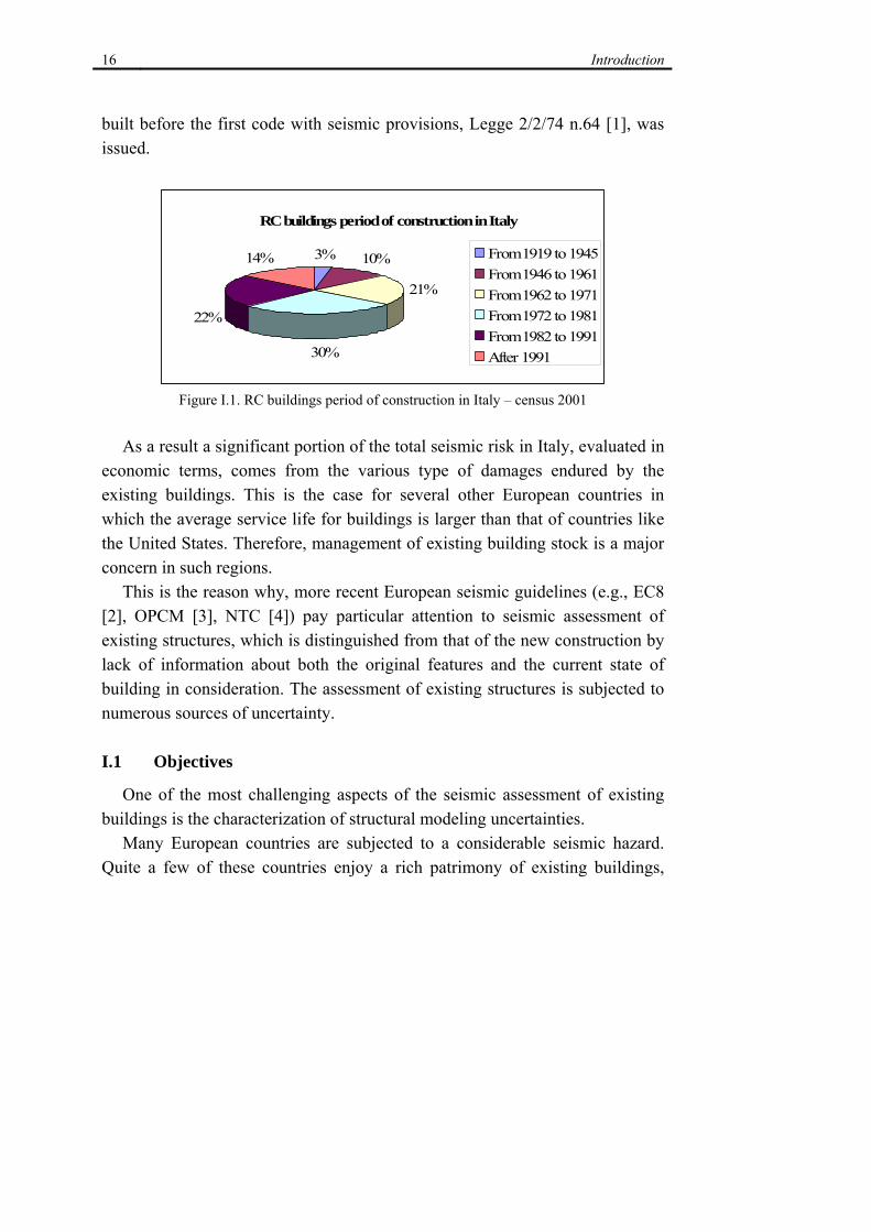
Moreover by analysing the data provided by the 14th census of population and buildings (2001) in Italy, it is possible to have a clear idea regarding the period of construction of the existing reinforced concrete buildings (see Figure I.1); such data show that about one million of building units (35%) have been
16 Introduction
built before the first code with seismic provisions, Legge 2/2/74 n.64 [1], was issued.
RC buildings period of construction in Italy
10%
21%
30%
22%
14% 3% From 1919 to 1945From 1946 to 1961From 1962 to 1971From 1972 to 1981From 1982 to 1991After 1991
Figure I.1. RC buildings period of construction in Italy – census 2001
As a result a significant portion of the total seismic risk in Italy, evaluated in
economic terms, comes from the various type of damages endured by the existing buildings. This is the case for several other European countries in which the average service life for buildings is larger than that of countries like the United States. Therefore, management of existing building stock is a major concern in such regions.
This is the reason why, more recent European seismic guidelines (e.g., EC8 [2], OPCM [3], NTC [4]) pay particular attention to seismic assessment of existing structures, which is distinguished from that of the new construction by lack of information about both the original features and the current state of building in consideration. The assessment of existing structures is subjected to numerous sources of uncertainty. I.1 Objectives
One of the most challenging aspects of the seismic assessment of existing buildings is the characterization of structural modeling uncertainties.
Many European countries are subjected to a considerable seismic hazard. Quite a few of these countries enjoy a rich patrimony of existing buildings,
Introduction 17
which for the most part were built before the specific seismic design provisions made their way into the constructions codes. Therefore, the existing buildings can potentially pose serious fatality and economic risks in the event of a strong earthquake. One very recent and very unfortunate case is the L’Aquila Earthquake of 6 April 2009 in central Italy. One main feature distinguishing the assessment of existing buildings from that of the new construction is the large amount of uncertainty present in determining the structural modeling parameters. Recent codes such as Eurocode 8 [2] seem to synthesize the effect of structural modeling uncertainties in the so-called confidence factors (CFs) that are applied to mean material property values. The confidence factors are classified and tabulated as a function of discrete knowledge levels acquired based on the results of specific in-situ tests and inspections.
With the emerging of probability-based concepts such as life-cycle cost analysis and performance-based design, the question arises as to what the CF would signify and would guarantee in terms of the structural seismic reliability [5,6]. This would not be possible without a thorough characterization of the uncertainties in the structural modeling parameters [5,7].
A fully probabilistic method coupled with non-linear dynamic analysis would be the best method in order to incorporate all relevant sources of uncertainties; however pragmatism oblige the adoption of a simplified format, calibrated on the fully probabilistic method, able to put the engineer in the condition to approach the problem by incorporating the uncertainties of different nature in the assessment procedure.
The objective of this thesis work is to investigate how dealing with the different sources of uncertainty that affect the assessment of existing RC buildings.
Methods alternative to the code based confidence factors are proposed and adopted for the case study structure.
These methods employ a Bayesian framework in order to update the global structural performance-based reliability in relation of different knowledge levels obtained for the analyzed structure.
18 Introduction
I.2 Problems of Existing RC Buildings
The problem of structural safety for existing buildings must be addressed by identifying the technical and social reasons that make a large number of buildings potentially at risk. The quality of constructions in Italy, especially in the last fifty years, is poor with respect to the constructions of the same period in other European country [8]. This situation is probably due to the “construction-boom” which gave rise, in the last fifty years, to a considerable urbanization phenomenon; this buildings, often unlawful, are characterized by insufficient design standards, lack of attention in structural details and use of poor quality materials. Most of reinforced concrete (RC) existing structures have been designed mainly for gravity loads and the seismic provisions considered in the design process are very poor or non-existent. In addition, this buildings, which are often subjected to load conditions not foreseen during the design process and used for purposes other than those they were designed for, may experience significant degradation.
The assessment of existing structures is distinguished from that of the new construction by lack of information about both the original features and the current state of building in consideration. In fact, design documentation for this buildings tends to be poor and original design calculations and working drawings usually are unavailable.
Even in cases in which the original documentation is available, it may be that, during the construction process (which is rarely subjected to quality control) something has been changed from the original documents due to lack of attention, unavailability of materials or speculative reasons. Furthermore design codes, materials and construction practices are changed, and material specifications may be difficult to obtain. Moreover not all members may be accessible for inspection and previous maintenance operation, even if conducted, may have caused undesirable strength and stiffness variations. In any case; full documentation relative to the maintenance operations performed in the past are often unavailable.
Introduction 19
In short determining the structural modelling parameters such as, materials properties and structural detailing parameters in existing RC structures is not an easy task and is subjected to a significant level of uncertainty.
I.3 Evolution of the Legislation and Practice Project
While new buildings are designed based on Performance-Based design principles, the existing buildings are designed based on an engineering conception founded on deterministic models of actions and resistances. Thus the structure would be verified only in relation to the maximum resistance of its composing structural elements.
Moreover, as stated previously, most of existing RC structures have been designed mainly for gravity loads and the seismic provisions considered in the design process are very poor or non-existent.
In fact the first identification of seismic zones in Italy, took place in early 900 through the instrument of the Regi Decreti, issued following the destructive earthquake of Messina and Reggio Calabria 28/12/1908. A list of the cities which were hit by the earthquake was compiled. The hit towns were divided into two categories, in relation to their degree of seismicity and their geological formation. After occurrence of each strong earthquake, the so-called list was updated by simply adding new towns affected by seismic event.
The first code in which was established a framework for classifying national seismic hazard with special requirements for seismic zones, as well as drafting of technical regulations, is the Legge 2/2/1974, n. 64 [1], “Provvedimenti per le costruzioni con particolari prescrizioni per le zone sismiche”.
It should be noted that the distinctive character of this law was the opportunity to update the rules whenever it was warranted by evolving knowledge of seismic phenomena; instead for the seismic classification was made, as in the past, simply by appending to the list the new towns affected by the new earthquakes.
Seismological characterizations conducted in the aftermath of the earthquakes of Friuli Venezia Giulia, 1976, and of Irpinia, 1980, have led to a significant increase in knowledge on the seismicity of the national territory and
20 Introduction
have led to a proposal for seismic classification of the national territory. This has been translated into a series of decrees approved between 1980 and 1984, which defined the Italian seismic classification, until the OPCM [3].
As much as it concerns the technical standards, the first seismic provisions were already enacted with the DM 3/3/1975 [9], subsequently supplemented by a series of successive decrees, with some relevant technical information contained in the accompanying ministerial circulars.
Immediately after the earthquake of 31 October 2002, which hit the territories on the border between the Molise and Puglia, the Department of Civil Protection (DPC) has adopted the OPCM [3], in order to provide an immediate response to the need for updating the seismic zonation and seismic provisions.
Among the major innovations of this new legislation, one can name the extension of the seismic zonation throughout the country, the replacement of the allowable stress method in favor of the limit state method of verification, and attention to proper structural modeling analysis.
Unlike the earlier seismic provisions, in the OPCM [3], and subsequent modifications, the entire national territory has been classified as seismic and is divided into 4 zones, characterized by decreasing seismic hazard; these areas have been identified by 4 classes of peak ground acceleration with a probability of exceedance of 10% in 50 years. In this new classification the three zones of high, medium and low seismicity, were provided the standards of seismic design with different levels of severity, while for zone 4, a new feature was introduced, which gave the regions the option to to require the standards for seismic design.
It should be stressed, moreover, the close link between the rules contained in the OPCM [3] and the system of laws already established in Europe, Eurocode 8 [2].
The main difference between the new generation codes, such as EC8 [2] and OPCM [3], and the traditional ones, is the substitution of conventional design and purely prescriptive approach with a performance-based approach in which the objectives of design are declared, and the set of rules and methods used for
Introduction 21
this purpose (the procedures for structural analysis and sizing of elements) are individually justified. Another innovative aspect of the OPCM [3] is that for the first time the problem of evaluation of existing structures was explicitly addressed and an entire chapter was dedicated to it.
Together with the DM 14/09/2005 [10] the “Technical standards for construction” have been approved, which represent a first attempt towards unification of a highly fragmented and inhomogeneous framework. In fact, the design and assessment criteria for various building types are all outlined in one text. This includes both the mechanical material properties and the definition of loading. In this uniform code, the set of external actions are fixed base on the level of safety to be achieved and the minimum performance expectations for structures.
Regarding the characterization of seismic actions the general approach introduced by OPCM [3] is maintained; however the operative design procedures described in detail in the OPCM [3] must be taken only as illustrative suggestions and are not obligatory.
Together with the DM 14/01/2008, the new “Technical standards for construction” (NTC) [4] is published that is the result of the revision of standards approved in 2005.
These new rules, which generally confirm the basic approach in the 2005 rules, introduce some changes and provide a series of clarifications on specific aspects, some of which were taken from OPCM [3] and its subsequent modifications. Among the most important change include; • the definition of seismic intensity parameters as a function of the
coordinates of the location and class of use of the building; • slight variations in load factors and their combination; • redefinition of the parameters relating to verification of the load-bearing
capacity of foundations; • redefinition of the shear capacity assessment for RC elements; • definition of design rules for performance-based design and the
parameters that govern the achievement of the high and low ductility classification;
22 Introduction
• changes in expressions of the structural factor (q); • recommendation of the use of static pushover analysis as
complementary or alternative method with respect to linear analysis methods for checking the safety of buildings subject to earthquake.
This research work has been developed during the last steps of the described code evolution, therefore we will refer to both the OPCM [3] and the NTC [4].
As stated previously, more recent European seismic guidelines pay particular attention to seismic assessment of existing structures. In particular, existing buildings are distinguished from those of the new design since the project reflects the state of knowledge at the time of construction and may contain conceptual flaws of various kinds including those related to the construction process. Moreover, these buildings may have been subjected to past earthquakes or other accidental actions whose effects are not evident. Consequently the assessment of existing structures appears highly sensitive to uncertainties that maybe comparable to those related to the representation of seismic ground motion.
European and Italian seismic guidelines synthesize the effect of structural modeling uncertainties in the so-called confidence factors (CF) which have to be applied to mean material properties, assumed a priori or obtained by performing in-situ tests on the structure. The primary scope for introduction of these confidence factors is to allow for a certain level of conservatism, through the use of material strength values smaller than that of the corresponding mean values determined based on available knowledge, in the seismic assessment of existing structures.
Evaluation of these confidence factors is based on three increasing levels of knowledge about the structure, each of which are required for specific sets of tests (destructive and non-destructive) and inspections. The quantity and quality of data collected determines the method of analysis and values of the confidence factor applicable to the properties of materials to use later on in the safety checks.
Introduction 23
In particular there are three levels of knowledge: • KL1 - Limited; • KL2 - Extended; • KL3 - Comprehensive.
The aspects that define the levels of knowledge are: - geometry, i.e., the geometric characteristics of structural elements; - structural details, namely, the quantity and the arrangement of steel
reinforcement, including the stirrup spacing and closure; - materials, i.e., the mechanical properties of materials.
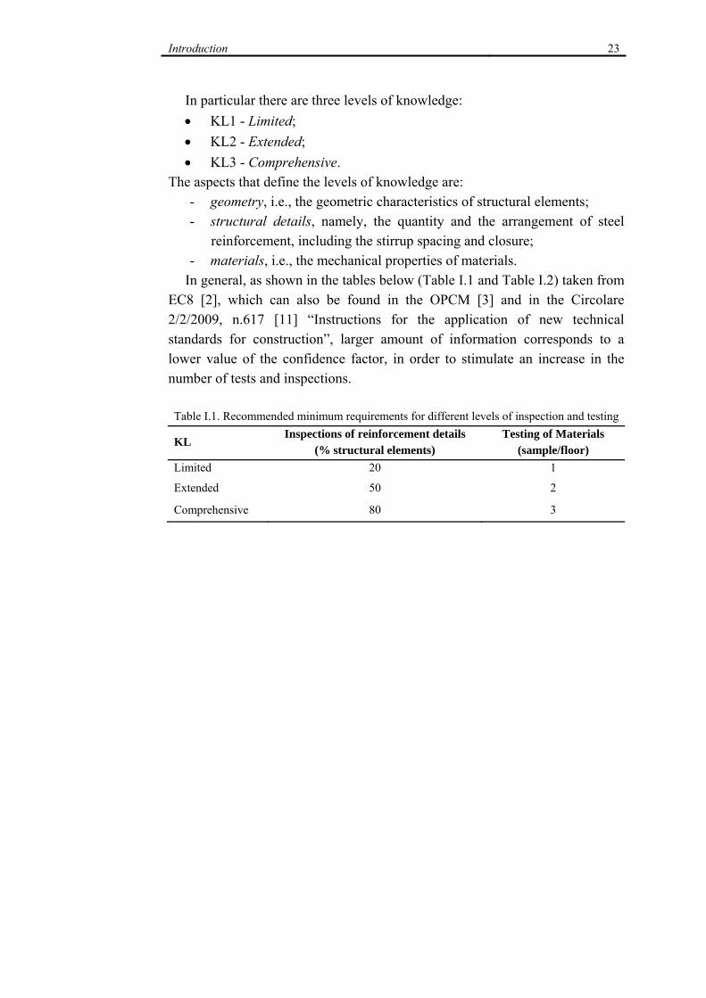
In general, as shown in the tables below (Table I.1 and Table I.2) taken from EC8 [2], which can also be found in the OPCM [3] and in the Circolare 2/2/2009, n.617 [11] “Instructions for the application of new technical standards for construction”, larger amount of information corresponds to a lower value of the confidence factor, in order to stimulate an increase in the number of tests and inspections. Table I.1. Recommended minimum requirements for different levels of inspection and testing
KL Inspections of reinforcement details
(% structural elements) Testing of Materials
(sample/floor) Limited 20 1
Extended 50 2
Comprehensive 80 3
24 Introduction
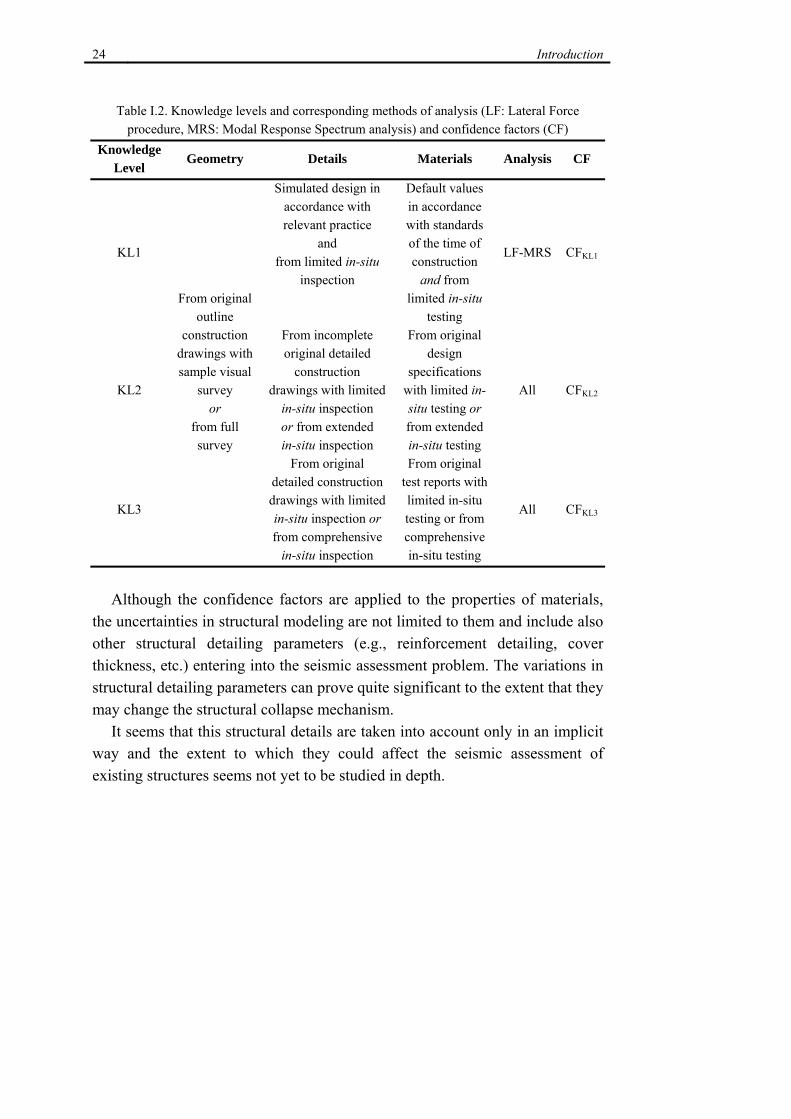
Table I.2. Knowledge levels and corresponding methods of analysis (LF: Lateral Force procedure, MRS: Modal Response Spectrum analysis) and confidence factors (CF)
Knowledge Level
Geometry Details Materials Analysis CF
KL1
From original outline
construction drawings with sample visual
survey or
from full survey
Simulated design in accordance with relevant practice
and from limited in-situ
inspection
Default values in accordance with standards of the time of construction
and from limited in-situ
testing
LF-MRS CFKL1
KL2
From incomplete original detailed
construction drawings with limited
in-situ inspection or from extended in-situ inspection
From original design
specifications with limited in-situ testing or from extended in-situ testing
All CFKL2
KL3
From original detailed construction drawings with limited in-situ inspection or from comprehensive
in-situ inspection
From original test reports with limited in-situ testing or from comprehensive in-situ testing
All CFKL3
Although the confidence factors are applied to the properties of materials,
the uncertainties in structural modeling are not limited to them and include also other structural detailing parameters (e.g., reinforcement detailing, cover thickness, etc.) entering into the seismic assessment problem. The variations in structural detailing parameters can prove quite significant to the extent that they may change the structural collapse mechanism.
It seems that this structural details are taken into account only in an implicit way and the extent to which they could affect the seismic assessment of existing structures seems not yet to be studied in depth.

Introduction 25
I.4 Evolution of Structural Materials
The importance of materials properties is evident in the approach prescribed for the assessment of existing buildings in the recent European and Italian seismic codes.
The mechanical properties of structural materials are important for sizing the elements in relation to the design action as well as for evaluating the structural capacity.
The material properties in an existing RC building can be determined from the following sources of information:
• common value used by the practice at the time of the construction; • original specifications of the original project or test certificates; • in-situ tests. The extent of in-situ tests depends on the chosen level of knowledge and on
other information available. Particularly important is the estimation of the concrete compressive strength
not only for the role it has on the load-bearing capacity and durability of the structure, but also because other properties of concrete such as the elastic modulus and tensile strength can be obtained directly or indirectly from it. In order to evaluate this quantity in existing RC structures, various methods of investigation both of destructive (i.e., involving localized removal of material as the carrot test) and non-destructive (e.g., rebound hammer test, ultrasonic test and the Sonreb combined method) nature can be used.
Moreover, chemical tests may be useful in order, for example, to detect the presence and the degree of carbonization, which can led to the corrosion of steel reinforcement.
It should be noted that these methods have undergone a substantial evolution in recent years but are efficient and reliable only when used properly. Nevertheless, a crucial role in the inspection process is still assumed by a visual direct examination [12].
The knowledge of historical data, namely the properties required by technical regulations in force at the construction time and / or quality of
26 Introduction
materials usually adopted in different periods of time and different regions, such as the specifications derived from the manuals (e.g., [13,14]), are very important for the estimation of material properties, especially reinforcing steel.
In fact the mechanical properties of steel are difficult to assess with non-destructive in-situ tests. Therefore their evaluations generally requires the removal of reinforcement to be tested later in the laboratory. These pieces have to be taken under particular conditions and from locations that would not compromise the integrity of the structural element and would minimize the resulting damage.
However both concrete and reinforcement steel mechanical properties have had a substantial improvement in quality and in performance, thanks to new technology for their production and also to the development of more severe acceptance criteria as a result of updating of constructions codes. I.5 Open Issues in the Current Code-Based Approach
At a first glance, the application of the confidence factor seems to be a deterministic method for addressing an inherently probabilistic problem.
In the code approach, the effect of the application of the confidence factors on structural reliability is not explicitly stated. Instead, with the emerging of probability-based concepts such as life-cycle cost analysis and performance-based design, the question arises as to what the CF would signify and would guarantee in terms of the structural seismic reliability [5,6]. This would not be possible without a thorough characterization of the uncertainties in the structural modeling parameters [5,7].
Another issue regards the definition of the level of knowledge (KL). The current code definition in Table I.2 leaves a lot of room for interpretation. For example, it does not explicitly specify the spatial configuration and the outcome of the test results. Moreover, the logical connection between the numerical values for the CFs and the onset of the KLs is not clear.
These problems underline the necessity of developing simple and approachable methods, based on structural reliability concepts, in order to
Introduction 27
assess the structural performance of existing RC structures in the presence of modeling uncertainties. I.6 Variability of the Assessment Results
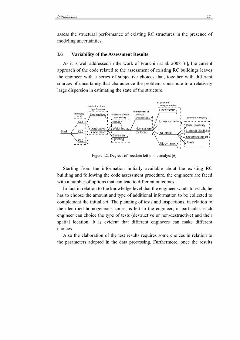
As it is well addressed in the work of Franchin at al. 2008 [6], the current approach of the code related to the assessment of existing RC buildings leaves the engineer with a series of subjective choices that, together with different sources of uncertainty that characterize the problem, contribute to a relatively large dispersion in estimating the state of the structure.
Figure I.2. Degrees of freedom left to the analyst [6].
Starting from the information initially available about the existing RC
building and following the code assessment procedure, the engineers are faced with a number of options that can lead to different outcomes.
In fact in relation to the knowledge level that the engineer wants to reach, he has to choose the amount and type of additional information to be collected to complement the initial set. The planning of tests and inspections, in relation to the identified homogeneous zones, is left to the engineer; in particular, each engineer can choice the type of tests (destructive or non-destructive) and their spatial location. It is evident that different engineers can make different choices.
Also the elaboration of the test results requires some choices in relation to the parameters adopted in the data processing. Furthermore, once the results
28 Introduction
have been collected, these have to be integrated with the initial data set. It could happen that the results contradict the initial data set: one engineer might accept the discrepancy, within certain limits, while another may choose to rely entirely on in-situ information adopting a comprehensive survey on the structure.
Therefore, for the same existing building, different engineers can obtain different structural models; moreover they could choose different analysis methods.
If the chosen analysis method is the dynamic one, another relevant source of uncertainty could affect the assessment results, that is the uncertainty in the representation of the ground motion. This source of uncertainty is strictly related to the selection of the ground motion records to be used in the structural assessment employing time-history analysis procedures. In fact, the seismic input selection represents one of the main issues in assessing the seismic response of a structure through numerical dynamic analysis; this choice may be affected by the interface variable used to measure the intensity of ground motion and may cause bias in assessment results.
Therefore, at the end of the assessment process, for the same existing RC structure we can have a large variability of results. I.7 The Organization of the Thesis
In this thesis the problem of the seismic assessment of existing RC buildings is addressed, with particular attention to the various sources of uncertainty associated with it.
In chapter I, different approaches to the structural safety problem are briefly presented and discussed. Particular attention is given to how dealing with uncertainties in engineering safety problems and decision making under uncertainty. The probability-based performance assessment framework is described in details.
In chapter II a review of some interesting research works concerning the problem of the seismic assessment of existing RC buildings, with particular attention to the confidence factors defined in the code, is presented. The relation between confidence factor and structural reliability for the case study
Introduction 29
structure is investigated accounting for both material properties uncertainty and structural detailing uncertainty. A proposal for a probability-based definition of confidence factor in relation to the global structural performance is presented.
In chapter III, the representation of ground motion in the seismic assessment and the uncertainties associated with it is discussed. A graphical and statistical tool is implemented in order to evaluate the fulfillment of the condition of sufficiency for different intensity measures adopted to represent the ground motion in the assessment; a simplified method using the statistical tool of the weighted regression is presented and adopted when this condition is not verified in order to modify the assessment of the structural performance in relation to the observed dependencies. The weights are assigned in relation to the results of the seismic hazard disaggregation for the site of interest.
In chapter IV an efficient simulation method that allows the robust estimation of the structural fragility with a small number of analysis is presented and implemented for the case study structure, accounting for the uncertainty in the materials properties and the construction detail parameters. The efficient simulation method is implemented using both static and dynamic non-linear analysis; in the case of dynamic analysis, also the uncertainty in the ground motion representation is taken into account.
In chapter V, in the framework of demand and capacity factor design, an alternative probabilistic-based formulation of the confidence factors for the estimation of structural safety of existing buildings is presented for both static and dynamic non-linear analysis procedures, in relation to different knowledge levels. The proposed approach, similar to that adopted by the SAC-FEMA guidelines [15], takes into account the uncertainty about the structural modeling parameters (materials and details), and those related to the ground motion representation. This alternative formulation is applied to the case study structure for different hypotheses related to the outcome of tests and inspections. A code-based implementation of the proposed alternative performance-based safety-checking format is presented.
Finally, in chapter VI a survey for professional engineers is presented in order to obtain a database based on expert opinion for characterizing prior

30 Introduction
probability distributions for structural details. Preliminary testing results obtained by interviewing a small group of professionals are presented.

Introduction 31
I.8 References
[1] Legge 2 febbraio 1974 n. 64, “Provvedimenti per le costruzioni con particolari prescrizioni per le zone sismiche” (in Italian).
[2] CEN, European Committee for Standardisation TC250/SC8/ [2003] “Eurocode 8: Design Provisions for Earthquake Resistance of Structures, Part 1.1: General rules, seismic actions and rules for buildings,” PrEN1998-1.
[3] Ordinanza del Presidente del Consiglio dei Ministri (OPCM) n. 3431, “Ulteriori modifiche ed integrazioni all'ordinanza del Presidente del Consiglio dei Ministri n. 3274 del 20 marzo 2003”. Gazzetta Ufficiale della Repubblica Italiana n. 107 del 10-5-2005 (Suppl. Ordinario n.85), 2005 (in Italian).
[4] CS..LL.PP, DM 14 gennaio, Norme Techniche per le Costruzioni (NTC). Gazzetta Ufficiale della Repubblica Italiana, 29, 2008 (in Italian).
[5] Jalayer F., Iervolino I., Manfredi G., “Structural modeling uncertainties and their influence on seismic assessment of existing RC structures”, submitted to Structural Safety, 2008.
[6] Franchin P., Pinto P. E., Pathmanathan R., Assessing the adequacy of a single confidence factor in accounting for epistemic uncertainty, Convegno RELUIS “Valutazione e riduzione della vulnerabilità sismica di edifici esistenti in cemento armato”, Roma 29-30 maggio 2008.
[7] Monti G., Alessandri S., Confidence factors for concrete and steel strength, Convegno RELUIS “Valutazione e riduzione della vulnerabilità sismica di edifici esistenti in cemento armato”, Roma 29-30 maggio 2008.
[8] “Valutazione riduzione della vulnerabilità sismica di edifici esistenti in cemento armato”, Cosenza E., Manfredi G., Monti G. editors, Polimetrica publisher, 2008.
[9] Decreto Ministero per i lavori pubblici, 3 marzo 1975, “Disposizioni concernenti l’applicazione delle norme tecniche per le costruzioni in zone sismiche”, (in Italian)..
[10] Decreto del Ministero delle infrastrutture e dei trasporti, 14 settembre 2005, “Norme Tecniche per le costruzioni”, (in Italian)..
[11] Circolare del Ministero delle infrastrutture e dei trasporti n.617, 2 febbraio 2009, “Istruzioni per l’applicazione delle Nuove norme tecniche delle costruzioni di cui al DM 14 gennaio 2008”, (in Italian)..

32 Introduction
[12] “Valutazione degli edifici esistenti in cemento armato”, G. Manfredi, A. Masi, R. Pinho, G. M. Verderame, M. Vona, Manuale IUSS Press, 2007.
[13] Santarella L. “Il cemento armato – Le applicazioni alle costruzioni civili ed industriali”, Edizione Hoepli 1968.
[14] Pagano M. “Teoria degli edifici - Edifici in cemento armato”, Napoli, Edizione Liguori 1968.
[15] Federal Emergency Management Agency (FEMA), 2000. Pre-Standard and Commentary for the Seismic Rehabilitation of Buildings. FEMA 356, Washington, D.C.
Chapter I – Approaches to Structural Safety Problems 33
Chapter I
Approaches to Structural Safety Problems
1. Introduction
Recent significant advances in the engineering design and the revolution in information technology and computing have made possible to predict the behavior and performance of complex engineered system with an increasing level of accuracy.
However numerous sources of uncertainties arise in the analysis and assessment process, causing a significant impact on technical, economic and social decisions. Some of these uncertainties stem from randomness inherent in nature, others arise from a lack of knowledge and ignorance. Both sources of uncertainty are equally important and must be considered in engineering safety problems [1].
The inevitable consequence of these uncertainties is that the engineering system may fail to perform as intended by the owner, occupant or user, or society as a whole.
It is not feasible to eliminate risk entirely; rather, the risk must be managed in the public interest by engineers, code bodies and political system.
Engineers traditionally have dealt with risk and uncertainty by making conservative assumptions in analysis and design, postulating worst-case scenarios, and applying factors of safety. Such approaches provide an unknown
34 Chapter I – Approaches to Structural Safety Problems
margin of safety against the failure state, however it is defined. Often, the decision is so conservative as to be wasteful of resources; occasionally, it errs in the non-conservative direction.
In recent years, there has been a growth in the use of reliability and risk analysis, founded in the mathematics of probabilistic and statistics, to support decision making in the presence of uncertainty. 2. Engineering Safety Problems
In this section a brief review of different approaches that can be used in order to solve engineering safety problems are presented. 2.1. Deterministic Approach
The first non-empirical approach to engineering safety problems is for sure the “allowable stress” method introduced at the beginning of 1900 and widely used till last few years. This approach consists in verifying that the maximum calculated tension in the most stressed section, in relation to the most unfavourable load condition, should be smaller than a certain allowable stress level. This allowable stress value is evaluated in relation to the material fracture stress, scaled by a safety factor that accounts for the uncertainties related to load and stress conditions. 2.2. Semi-Probabilistic Approach
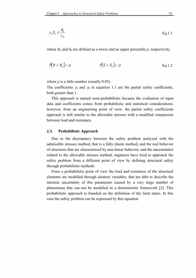
Recent codes and provisions have introduced the evaluation of structural safety through a semi-probabilistic approach based on the definition of the limit states; this approach is closer to the probabilistic one, that will be discussed later, but is based on the introduction of partial safety coefficients to the characteristic values of the load and resistance. This approach is also known as the first level method.
Within this method the engineer has only to ensure that:
Chapter I – Approaches to Structural Safety Problems 35
R
kkS
RSγ
γ ≤ Eq.1.1
where Rk and Sk are defined as a lower and an upper percentile p, respectively.
[ ] pRRP k =< [ ] pSSP k => Eq.1.2
where p is a little number (usually 0.05). The coefficients γS and γR in equation 1.1 are the partial safety coefficients, both greater than 1.
This approach is named semi-probabilistic because the evaluation of input data and coefficients comes from probabilistic and statistical considerations; however, from an engineering point of view, the partial safety coefficients approach is still similar to the allowable stresses with a modified comparsion between load and resistance. 2.3. Probabilistic Approach
Due to the discrepancy between the safety problem analyzed with the admissible stresses method, that is a fully elastic method, and the real behavior of structures that are characterized by non-linear behavior, and the uncertainties related to the allowable stresses method, engineers have tried to approach the safety problem from a different point of view by defining structural safety through probabilistic methods.
From a probabilistic point of view the load and resistance of the structural elements are modelled through aleatory variables, that are able to describe the intrinsic uncertainty of this parameters caused by a very large number of phenomena that can not be modelled in a deterministic framework [2]. This probabilistic approach is founded on the definition of the limit states. In this case the safety problem can be expressed by this equation:
36 Chapter I – Approaches to Structural Safety Problems
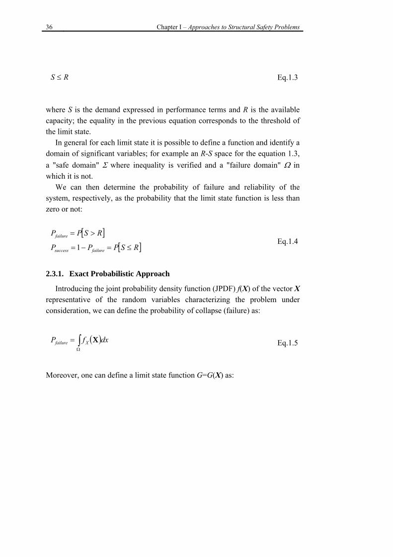
RS ≤ Eq.1.3
where S is the demand expressed in performance terms and R is the available capacity; the equality in the previous equation corresponds to the threshold of the limit state.
In general for each limit state it is possible to define a function and identify a domain of significant variables; for example an R-S space for the equation 1.3, a "safe domain" Σ where inequality is verified and a "failure domain" Ω in which it is not.
We can then determine the probability of failure and reliability of the system, respectively, as the probability that the limit state function is less than zero or not:
[ ]RSPPfailure >=
[ ]RSPPP failuresuccess ≤=−= 1 Eq.1.4
2.3.1. Exact Probabilistic Approach
Introducing the joint probability density function (JPDF) f(X) of the vector X representative of the random variables characterizing the problem under consideration, we can define the probability of collapse (failure) as:
( )dxfP Xfailure X∫Ω
= Eq.1.5
Moreover, one can define a limit state function G=G(X) as:
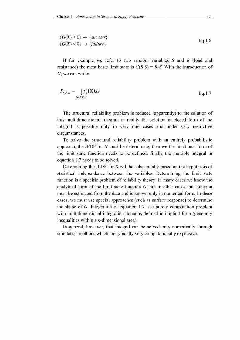
Chapter I – Approaches to Structural Safety Problems 37
G(X) > 0 → success G(X) < 0 → failure
Eq.1.6
If for example we refer to two random variables S and R (load and
resistance) the most basic limit state is G(R,S) = R-S. With the introduction of G, we can write:
( )dxfPG
Xfailure XX∫
≤
=0)(
Eq.1.7
The structural reliability problem is reduced (apparently) to the solution of
this multidimensional integral; in reality the solution in closed form of the integral is possible only in very rare cases and under very restrictive circumstances.
To solve the structural reliability problem with an entirely probabilistic approach, the JPDF for X must be determinate; then we the functional form of the limit state function needs to be defined; finally the multiple integral in equation 1.7 needs to be solved.
Determining the JPDF for X will be substantially based on the hypothesis of statistical independence between the variables. Determining the limit state function is a specific problem of reliability theory: in many cases we know the analytical form of the limit state function G, but in other cases this function must be estimated from the data and is known only in numerical form. In these cases, we must use special approaches (such as surface response) to determine the shape of G. Integration of equation 1.7 is a purely computation problem with multidimensional integration domains defined in implicit form (generally inequalities within a n-dimensional area).
In general, however, that integral can be solved only numerically through simulation methods which are typically very computationally expensive.
38 Chapter I – Approaches to Structural Safety Problems
However in the case of the two-dimensional problem of independent load and resistance variables and linear limit state function, it is possible to find a closed form solution of the integral.
For example in the case of the formulation of structural reliability problem based on the limit state function defined as G(R,S) = R-S, where R and S are independent variables for which the functions of marginal probability density PDFs (Probability Density Functions), fR(r) and fS(s), are known, equation 1.7 can be written in this form:
[ ]∫∫
<−
==0
, ),(SR
SRffailure drdssrfPP Eq.1.8
Since the independence of the variables we can write:
( ) ( )sfrfsrf SRSR =),(, Eq.1.9
and by substitution in equation 1.8:
[ ]( ) ( ) ( )∫∫ ∫∫∫
∞∞
<−
=⎥⎦
⎤⎢⎣
⎡==
00 00, )(),( dssFsfdsdrrfsfdrdssrfP RS
s
RSSR
SRf Eq.1.10
and then the probability of failure is given by the convolution integral of two functions of s, where fS(s) is the PDF of S and FR(s)=P[R<S] is the CDF (Cumulative Distribution Function) of R.
In general, cases where the integral is solved analytically coming to the exact solution are extremely rare. However, there are numerical methods for solving the problem of calculating the probability of failure. These simulation methods sample the variables in the safety-checking problem from their JPDF.

Chapter I – Approaches to Structural Safety Problems 39
For each realization of these variables, the limit state function is checked to see whether the sample lies in the failure space or not. These procedures, more or less refined, are all characterized by an accuracy inversely proportional to the number of simulations.
The easier simulation method, but also the best known, is the so-called Monte Carlo method. It calculates the integral defining an auxiliary function I, called indicator function, which takes the value zero for values of the vector X for which the limit state function G is positive (safe space) and unit value for values of the vector X for which the limit state function takes negative values (failure space).
⎩⎨⎧
≤>
=0)(10)(0
)(XX
XGifGif
I Eq.1.11
The indicator function is used to calculate the probability of collapse by
extending the integral to the whole space of definition of X, thus overcoming the problem of having to determine the failure domain Ω. It can be shown that, in this way, the integral in equation 1.7 is approximated by the ratio between the number of repetitions of the experiment that have given a negative result (Nf) and the total number of tests performed.
TOT
f
RXXf N
NdXfIdXfP
n
≅== ∫∫Ω
)()()( XXX Eq.1.12
It can be shown that the coefficient of variation of probability of collapse is
equal to the following expression:
PfNPfPVOC f ⋅
−=
1).(.. Eq.1.13
40 Chapter I – Approaches to Structural Safety Problems
Therefore, for example in order to estimate a probability of collapse equal to
10-3 with a coefficient of variation around 30%, one needs to perform at least 104 simulations .
Since the probability of collapse in structures is generally very small and each simulation requires a complete structural analysis, the computational effort can be prohibitive even for computers. Therefore alternative simulation methods, called smart simulation methods, have been developed. Generally speaking, these methods represent modifications of the Monte Carlo method in order to try to reduce the number of simulations needed to calculate the reliability with a given accuracy. 2.3.2. Simplified Probabilistic Approach
The integral in equation 1.5 in most cases can only be solved numerically. As described in the previous section, numerous numerical simulations will result very costly in terms of time and computing power.
As stated before, the main problems related to the calculation of the integral can be summarized as follows [3]: 1) the domain of integration is known only in implicit form; 2) the domain of integration is generally "far" from the mean of the vector X; 3) the integrand may have a steep slope in the domain of integration. The first point makes it difficult to find the limits (bounds) for the domain of integration. The second point makes it difficult to efficiently generate the random numbers, while the third point requires an accurate choice of the integration pattern in order to avoid losing some peak value of the integrand. For these reasons, several authors have proposed the idea of assess the reliability with an index β, called reliability index [4]. This index measures, in units of standard deviation, the distance between the average value of the vector X and the boundary of the domain of failure, or the distance between this average value and the point of the limit state function (G(X)=0) which is closest
Chapter I – Approaches to Structural Safety Problems 41
to the average value (design point). The evaluation of the index β is therefore a constrained minimization problem.
Once this index has been calculated, it is possible to calculate the probability of collapse and compare it with the reference values to assess the degree of reliability of the structure, obviously the greater the value of β, the lower the probability of collapse.
In the case of the load-resistance model, assuming that the vector of random variables R and S is normally distributed, the function G = R-S is still normally distributed. Assuming that R and S are also uncorrelated, the mean and standard deviation of G are given by:
SRG µµµ −= 22SRG σσσ +=
Eq.1.14
In this particular case the probability of collapse can be calculated simply by
recalling the Gauss integral:
( ) ( )βΦ−=β−Φ=⎟⎟
⎠
⎞
⎜⎜
⎝
⎛
σ+σ
µ−µ−Φ=
πσ= ∫
∞−
⎟⎟⎠
⎞⎜⎜⎝
⎛σ
µ−−
12
122
021
2
SR
SR
g
Gf dgeP G
G
Eq.1.15
where β is the value at which the Gaussian function is calculated in order to obtain the probability of collapse. This result is susceptible to a geometric interpretation: indeed posing y2=(r-µR)/σR and y1=(s-µS)/σS, the limit state function can be expressed as follows:
SRSR yySRG µµσσ −+−= 12),( Eq.1.16
42 Chapter I – Approaches to Structural Safety Problems
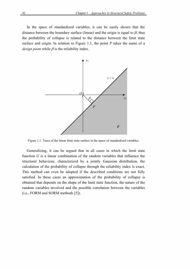
In the space of standardized variables, it can be easily shown that the distance between the boundary surface (linear) and the origin is equal to β; thus the probability of collapse is related to the distance between the limit state surface and origin. In relation to Figure 1.1, the point P takes the name of a design point while β is the reliability index.
. Figure 1.1. Trace of the linear limit state surface in the space of standardized variables.
Generalizing, it can be argued that in all cases in which the limit state
function G is a linear combination of the random variables that influence the structural behaviour, characterized by a jointly Gaussian distribution, the calculation of the probability of collapse through the reliability index is exact. This method can even be adopted if the described conditions are not fully satisfied. In these cases an approximation of the probability of collapse is obtained that depends on the shape of the limit state function, the nature of the random variables involved and the possible correlation between the variables (i.e., FORM and SORM methods [5]).
y1
P
O β
r = s
F
y2
Chapter I – Approaches to Structural Safety Problems 43
3. Aleatory and Epistemic Uncertainties
It is common in risk analysis and engineering safety problems to distinguish between uncertainty that reflects the variability of the outcome of a repeatable experiment (aleatory uncertainty) and uncertainty due to limited or imperfect knowledge (epistemic uncertainty). The times and magnitudes of future earthquakes in a region, record-to-record variability in acceleration time-history amplitudes and phases are examples of the former type, while uncertainty on the age of the universe, the geologic profile of a site, or the earthquake capability of a fault are examples of the latter [1].
It may thus appear that the labeling of any given uncertainty as aleatory or epistemic is self-evident, but in fact the aleatory/epistemic quality is not an absolute attribute of uncertainty. Rather, it depends on the deterministic or stochastic representation that we make of a phenomenon [6].
However, the importance of distinguishing between aleatory and epistemic uncertainty it is not relevant for decision making, but serves the useful practical purpose of forcing the analyst to consider all sources of uncertainty. 4. Statistical and Non-Statistical Information
In essence, uncertainty about the applicable model (and its parameters) is epistemic, whereas uncertainty given the model (and its parameters) is aleatory.
Classical and Bayesian statistics handle epistemic uncertainty in different ways. In Bayesian statistics one first identifies the set of plausible models and then assigns to each model a probability of being correct based on all available information. In principle, the initial selection of models can be arbitrarily broad, since the implausible models can subsequently be assigned zero probability, without affecting the final result.
By contrast, classical statistics does not assign probabilities to models and deals exclusively with statistical data (with information in the form of outcomes of statistical experiments). Any non-statistical information (for example theoretical arguments, physical constraints, expert opinion) constrains
44 Chapter I – Approaches to Structural Safety Problems
the set of plausible models, but is not subsequently used to quantify uncertainty within the chosen set of models.
Therefore, the selection of plausible models is usually a more sensitive operation in classical statistics than in Bayesian statistics. 5. Decision Making Under Uncertainty
There are two main approaches to decision making under uncertainty, namely classical decision theory and Bayesian decision theory. Bayesian decision theory is conceptually simpler because it treats aleatory and epistemic uncertainty in the same way. It is also the more broadly applicable one, because as previously noted it can handle also non-statistical information. 5.1. Bayesian Decision Theory
In this framework a utility function can be defined to express the relative desirability of alternative actions (e.g. seismic design decisions) taken when confronting with possible future events (future earthquakes and their consequences). An action is then considered optimal if it maximizes the expected utility relative to all uncertain quantities. Bayesian decision theory involves three basic steps: 1. Identify all uncertain quantities that affect the utility U(A) for each action A.
We denote by X the vector of such uncertain quantities. 2. Quantify uncertainty on (X|D). This is done by separately considering
statistical and non-statistical information. Non-statistical information is used to produce a prior distribution of X (“the prior”). Statistical data are subsequently accounted for by calculating the likelihood of (X|D). The posterior distribution of (X|D) is given by the normalized product of the prior and the likelihood function:
)()(
)|()|( XPDP
XDPDXP = Eq.1.17
Chapter I – Approaches to Structural Safety Problems 45
3. Specify a utility function U(A,X) to measure the relative desirability of alternative (A,X) combinations. Decisions are ranked according to the utility U(A), given by:
∫=allX
DX xdFAxUAU )(),()( | Eq.1.18
where FX|D is the posterior distribution of (X|D). Hence, a decision A* is considered optimal if it maximizes U(A) in equation 1.18 [1].
It should be noted that the posterior distribution accounts for all available information on (X|D), whether statistical or not, and all uncertainty, whether aleatory or epistemic. Hence neither of these distinctions is influential on the decision and all that ultimately matters is the total uncertainty. 5.2. Classical Decision Theory
Classical decision analysis differs from Bayesian decision analysis in that it does not represent quantities with epistemic uncertainty as random variables. While this leads to certain complications and limitations, decisions involving epistemic uncertainty can still be made.
Contrary to the Bayesian case, non-statistical information cannot be incorporated in the decision-making problem.
However, for complex decision problems, the classical procedure becomes inadequate, first of all because in cases that involve many random variables and uncertain parameters (for example in earthquake loss estimation problems, which combine earthquake recurrence, attenuation, system response and damage models) it may be difficult to define functions with distributions that do not depend on the unknown parameters. In these cases a practical way to make decisions is to set the unknown parameters to conservative values such as upper or lower confidence limits. This “confidence approach” is frequently used in practice, but is not satisfactory since there is no objective way to choose the acceptable level of confidence.
46 Chapter I – Approaches to Structural Safety Problems
6. The Total Probability Theorem
The total probability theorem is one of the most useful theorems of the probability theory. Given a set of mutually exclusive and collectively exhaustive events, B1, B2, …, Bn, the probability P[A] of another event A can always be expanded in terms of the following joint probabilities:
][]|[][1
i
n
ii BPBAPAP ⋅= ∑
= Eq.1.19
7. Probabilistic performance-based assessment
This section focuses on the general performance assessment methodology developed by Pacific Earthquake Engineering Research (PEER) Center for buildings in the framework of Performance-Based Earthquake Engineering (PBEE). The approach is aimed at improving decision making related to seismic risk associated with direct losses, downtime and life safety [7]. 7.1. Decision Variables
By definition PBEE is based on achieving desired performance objectives that are of concern to society as a whole or to specific groups or individual owners, such as life safety, dollar losses and downtime (or loss of function). It is postulated that the performance objective can be expressed in terms of a quantifiable entity and, for instance, its annual probability of exceedance. For instance the mean annual frequency1 (MAF) of collapse, or of the loss exceeding a certain quantity y of dollars, can be used as performance objectives. The quantifiable entities, on which the performance assessment is based, are referred to as decision variables (DVs). In the assessment methodology the key issue is to identify and quantify decision variables of
1 The MAF is approximately equal to the annual probability for the small probability values
of interest here.
Chapter I – Approaches to Structural Safety Problems 47
primary interest for the decision makers, with due consideration given to all important uncertainties.
In order to compute DVs and their uncertainties, other variables that define the seismic hazard, the demands imposed on the building systems by the hazard and the state of damage have to be defined and evaluated. 7.2. Intensity Measures
The seismic hazard is quantified in terms of a vector of intensity measures (IMs), which should comprehensively define the seismic input to the structure.
The vector can have a single component (scalar IM), such as spectral acceleration at the first mode period of the structure, Sa(T1), or can have several components [8], as it will be discussed in chapter III. If a scalar IM is adopted, such as Sa(T1), the hazard is usually defined in terms of a hazard curve.
The outcome of hazard analysis, which forms the input to demand evaluation, is usually expressed in terms of the MAF of exceeding the IM vector and denoted by λ(IM). 7.3. Engineering Demand Parameters
Given ground motion hazard, a vector of engineering demand parameters (EDPs) needs to be computed, which define the response of the building in terms of parameters that can be related to DVs. Relationships between EDPs and IMs are typically obtained through non-linear time-history analyses of the structure subject to a set of ground motion records. The outcome of this process, which may be referred to as probabilistic seismic demand analysis, can be expressed as G(EDP|IM) or more specifically as G[EDP ≥ y | IM = x], which is the probability that the EDP exceeds a specified value y, given (conditional) that the IM is equal to a particular value x.
48 Chapter I – Approaches to Structural Safety Problems
7.4. Damage Measures
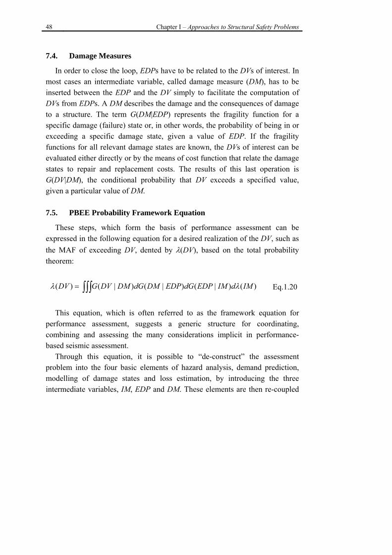
In order to close the loop, EDPs have to be related to the DVs of interest. In most cases an intermediate variable, called damage measure (DM), has to be inserted between the EDP and the DV simply to facilitate the computation of DVs from EDPs. A DM describes the damage and the consequences of damage to a structure. The term G(DM|EDP) represents the fragility function for a specific damage (failure) state or, in other words, the probability of being in or exceeding a specific damage state, given a value of EDP. If the fragility functions for all relevant damage states are known, the DVs of interest can be evaluated either directly or by the means of cost function that relate the damage states to repair and replacement costs. The results of this last operation is G(DV|DM), the conditional probability that DV exceeds a specified value, given a particular value of DM. 7.5. PBEE Probability Framework Equation
These steps, which form the basis of performance assessment can be expressed in the following equation for a desired realization of the DV, such as the MAF of exceeding DV, dented by λ(DV), based on the total probability theorem:
∫∫∫= )()|()|()|()( IMdIMEDPdGEDPDMdGDMDVGDV λλ Eq.1.20
This equation, which is often referred to as the framework equation for
performance assessment, suggests a generic structure for coordinating, combining and assessing the many considerations implicit in performance-based seismic assessment.
Through this equation, it is possible to “de-construct” the assessment problem into the four basic elements of hazard analysis, demand prediction, modelling of damage states and loss estimation, by introducing the three intermediate variables, IM, EDP and DM. These elements are then re-coupled

Chapter I – Approaches to Structural Safety Problems 49
by integration over all levels of the selected intermediate variables [7]. This integration required that the conditional probabilities G(EDP|IM), G(DM|EDP) and G(DV|DM) must be characterized over a suitable range of DM, EDP and IM levels.
The form of equation 1.20 implies that the intermediate variables (DMs and EDPs) are chosen such that the conditional probabilities are independent of one another and conditioning information need to be carried forward. This implies, for example, that given the structural response described by EDP, the damage measures (DMs) are conditionally independent of the ground motion intensity (IM), i.e., there are no significant effects of ground motion that influence damage and are not reflected in the calculated EDPs. The same can be said about the conditional independence of the decision variables (DV) from ground motion IM or structural EDP, given G(DV|DM). Likewise, the intensity measure (IM) should be chosen such that the structural response (EDP) is not also further influenced by, say, magnitude or distance, which have already been integrated into the determination of dλ(IM). Apart from facilitating the probability calculation, this independence of parameters serves to compartmentalize discipline-specific knowledge necessary to evaluate relationships between the key variables.

50 Chapter I – Approaches to Structural Safety Problems
8. References
[1] Y. K. Wen, B. R. Ellingwood, D. Veneziano, and J. Bracci “Uncertainty Modeling in Earthquake Engineering”, MAE Center Project FD-2 Report February 12, 2003.
[2] O. Ditlevsen, H.O. Madsen, “Structural Reliability Methods”, John Wiley & Sons Ltd, Chichester, 1996
[3] F. Casciati, J. Roberts, “Models for structural reliability analysis”, CRC Press, 1996.
[4] C.A. Cornell, “Bounds on the reliability of structural systems”, Journal ofstructural division, ASCE, Vo. 93, No. ST1, February 1967.
[5] C.A. Cornell, “A probability based structural code”, J. Am. Concr. Inst., 66, pp.974-985, 1969.
[6] W. M. Bulleit, “Uncertainty in Structural Engineering”, Practice Periodical on Structural Design and Construction, Vol. 13, No. 1, February 1, 2008. ©ASCE.
[7] G.G. Deierlein, H. Krawinkler, and C.A. Cornell, “A framework for performance-based earthquake engineering”, Pacific Conference on Earthquake Engineering (2003).
[8] J. W. Baker, C. A. Cornell, “Uncertainty propagation in probabilistic seismic loss estimation”, Structural Safety 30 (2008) 236–252.
51 Chapter II – Confidence Factor: the State of Research
Chapter II
Confidence Factor: the State of Research
1. Some Interesting Works
As it has been stressed in the introduction of this thesis, the problem of the assessment of existing RC buildings is of primary concern, not only for the engineers, but also for the political and research world. In fact the Italian Civil Protection has financed through RELUIS (Rete Laboratori Universitari di Ingegneria Sismica) different scientific tasks concerning the evaluation and reduction of seismic vulnerability of existing reinforced concrete buildings. In particular, a special task has been dedicated to the confidence factors.
In this context, some interesting works have addressed the open issues in the current code-based approach, obviously analyzing the problems from different points of view.
In particular, in the work of G. Monti and S. Alessandri (2008) [1], the authors chose to distinguish information about the strength of materials, that is affected by both inherent and epistemic uncertainties, from the information relative to construction details, affected only by epistemic uncertainties. For this reason a different approach has been proposed, in which confidence factors are evaluated separately for each material type. In particular, a method is proposed for the calibration of CF’s for the resistance of materials based on a Bayesian framework. This method allows to use the results obtained from
52 Chapter II – Confidence Factor: the State of Research
destructive and non-destructive tests to update the a priori probability distribution, taking into account the accuracy of individual tests. Thus a benchmark for the strength of materials is obtained in relation to a lower level percentile of the updated probability distribution for material properties.
The work by G. Monti and S. Alessandri focus on materials and evaluate the CF’s for different material properties. This CF’s are calibrated based on the material’s resistance and not on the global response of the structure.
In the work developed by P. Franchin et al.(2009) [2] a single value of the CF was adopted, taking into account all types of uncertainty. A reference structure was created in order to represent the complete state of knowledge and several realization of structural models were generated in which, for each knowledge level, the structure was known partially. The paper discusses the fact that, for each given level of knowledge, every analyst can develop a different (incomplete) picture of the structure. This way, probability distributions for the global response of the structure can be constructed , representing the variability of the choices each analyst can make (adhering to code specifications). The confidence factor was calibrated by setting a chosen lower percentile of the response value (say 10%) equal to one (the onset of collapse limit state).
The following describes, a fully probabilistic method for the assessment of the structural response developed by Jalayer et al. ([3,4]). This method calibrates the CF based on the probability distribution for the variable that describes the global performance of the structure, accounting for the uncertainties involved in the analysis of an existing structure. The uncertainties related to seismic motion were not taken into account in this work in order to use the typical analysis tools for the professional engineers: the static push-over and the capacity spectrum method [5] (Appendix C). 2. Confidence Factor and Structural Reliability
As mentioned in the precedent section, in a previous work by Jalayer et al., 2008 [4], here briefly presented and discussed, the authors have strived to quantify and to update both the modeling uncertainties and the structural
Chapter II – Confidence Factor: the State of Research 53
reliability for a case-study existing RC building, given the state of knowledge about the existing structure and given a specific level of seismic intensity, inside a Bayesian probabilistic framework. The focus of the study is on the uncertain parameters that are specific to an existing building as opposed to a building of new construction; thus, the uncertainties in the seismic action and the modeling uncertainties in the component capacities (e.g., the modeling uncertainty in determining the ultimate rotation in a section) were not taken into account.
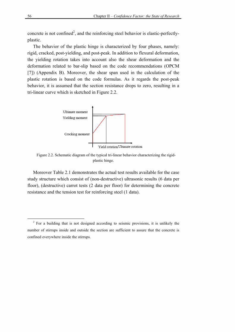
The characterization of uncertainties in this framework is preformed in two levels. In the first level, prior probability distributions for the uncertain modeling parameters are constructed based on information available from original design documents and professional judgment. In the second level, the results of in-situ tests and inspections are implemented in the Bayesian framework in order to both update the prior distributions for the modeling parameters and also to update the distribution for structural reliability using simulation-based reliability methods. The Bayesian updating procedure employed allows for updating the probability distributions for both structural modeling parameters and the structural global response within the simulation routine. Moreover, it is general enough to allow for both consideration of various types of inspections ranging from carrot tests, pacometric tests to pseudo-dynamic health-monitoring tests and also consideration of the corresponding measurement errors.
The updating of structural reliability across increasing amount of test results makes the authors able to, (i) introduce a performance-based probabilistic definition of the confidence factor as the value that, once applied to the mean material properties, leads to a value for structural performance measure with a specified probability of being exceeded (e.g., 5%), (ii) evaluate the code-based recommendations regarding confidence factors and the corresponding knowledge levels. The methodology presented allows for characterizing structural modeling uncertainties specific to existing buildings using a rigorous probabilistic framework. The relevant information has been implemented in
54 Chapter II – Confidence Factor: the State of Research
this framework in order to update both the modeling uncertainties and the probabilistic performance assessments. 2.1. The Case-Study Structure
As the case-study, an existing school building in the city of Avellino, Italy, is considered herein. Avellino is a city located in the Irpinia region, which is an historical and geographical region of central-southern of Italy. This region is notorious for the Irpinia Earthquake, that occurred on 23th of November 1980 and struck the central Campania and Basilicata. Characterized by a magnitude 6.9 on the Richter scale, with its epicenter in the town of Conza (AV), caused about 280,000 displaced persons, 8848 injured and 2914 deaths.
The Irpinia region was classified in the Italian seismic guidelines OPCM [6, 7] as seismic zone II. According to this classification, for this seismic zone a value of 0.25g is indicated for the maximum horizontal acceleration on the soil category A, with a probability of exceedance equal to 10% in 50 years.
The structure consists of three stories and a semi-embedded story and its foundation lies on soil type B. For the structure in question, the original design notes and graphics have been gathered.
The building is constructed in the 1960's and it is designed for gravity loads only, as it is frequently encountered in the post second world war construction.
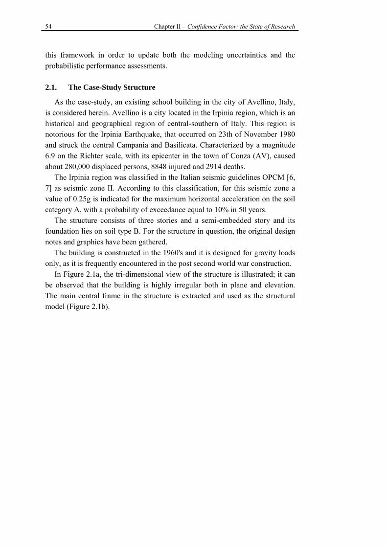
In Figure 2.1a, the tri-dimensional view of the structure is illustrated; it can be observed that the building is highly irregular both in plane and elevation. The main central frame in the structure is extracted and used as the structural model (Figure 2.1b).
Chapter II – Confidence Factor: the State of Research 55
XY XZY Z
(a)
(IV)
(III)
(II)
(I)
(1) (2) (3) (4)
3.50
m3.
90 m
3.90
m2.
20 m
4.20 m 4.20 m 4.20 m 3.50 m
(b) Figure 2.1: (a) The tri-dimensional view of the scholastic building (b) The central frame of
the case-study building
The columns have rectangular sections with the following dimensions: first storey: 40x55 cm2, second storey: 40x45 cm2, third storey: 40x40 cm2, and forth storey: 30x40 cm2. The beams, also with rectangular section, have the following dimensions: 40x70 cm2 at first and second floors, and 30x50 cm2 for the ultimate two floors.
It can be inferred from the original design notes that the steel rebar is of the type Aq42 (nominal minimum yield resistance fy = 2700 kg/cm2) and the concrete has a minimum resistance equal to 180 kg/cm2 (R.D.L. 2229, 1939 [8]).
The finite element model of the frame is constructed assuming that the non-linear behavior in the structure is concentrated in plastic hinges located at the element ends (Appendix A). Each beam or column element is modeled by coupling in series of an elastic element and two rigid-plastic elements (hinges). The stiffness of the rigid-plastic element is defined by its moment-rotation relation which is derived by analyzing the reinforced concrete section at the hinge location. In this study, the section analysis is based on the Mander-Priestly [9] constitutive relation for reinforced concrete, assuming that the
56 Chapter II – Confidence Factor: the State of Research
concrete is not confined2, and the reinforcing steel behavior is elastic-perfectly-plastic.
The behavior of the plastic hinge is characterized by four phases, namely: rigid, cracked, post-yielding, and post-peak. In addition to flexural deformation, the yielding rotation takes into account also the shear deformation and the deformation related to bar-slip based on the code recommendations (OPCM [7]) (Appendix B). Moreover, the shear span used in the calculation of the plastic rotation is based on the code formulas. As it regards the post-peak behavior, it is assumed that the section resistance drops to zero, resulting in a tri-linear curve which is sketched in Figure 2.2.
Figure 2.2. Schematic diagram of the typical tri-linear behavior characterizing the rigid-
plastic hinge.
Moreover Table 2.1 demonstrates the actual test results available for the case study structure which consist of (non-destructive) ultrasonic results (6 data per floor), (destructive) carrot tests (2 data per floor) for determining the concrete resistance and the tension test for reinforcing steel (1 data).
2 For a building that is not designed according to seismic provisions, it is unlikely the
number of stirrups inside and outside the section are sufficient to assure that the concrete is
confined everywhere inside the stirrups.
Chapter II – Confidence Factor: the State of Research 57
Table 2.1.Test results available for the structure
Test # data Type Standard Error
Carrot test Basement 2 destructive 0.150
Carrot test Ground floor 2 destructive 0.150
Carrot test Fisrt floor 2 destructive 0.150
Ultrasonic test Basement 6 non-destructive 0.335
Ultrasonic test Ground floor 6 non-destructive 0.335
Ultrasonic test First floor 6 non-destructive 0.335
Tension test Reinforcing steel 1 destructive 0.080
It should be noted that the standard error assigned to the ultrasonic tests is
larger than that assigned to the carrot tests to take into account the fact that the ultrasonic results are calibrated (using regression analysis) with respect to the carrot tests. 2.2. Evaluation of Robust Reliability
In the presence of structural modeling uncertainty, instead of a unique structural model, a set of plausible structural models can be identified. A robust assessment of structural reliability takes into account a whole set of possible structural models that are weighted by their corresponding plausibility. A Bayesian updating framework can be implemented in order to update both the structural modeling properties and the reliability based on test results [10]. Nevertheless, model updating is not an end by itself, and it is normally desirable to also improve the predictions of structural reliability.
Let the vector θ denote the set of uncertain model parameters. Let D denote some test data and consider that the set of possible structural models can be defined by M to specify (both the structural and the probabilistic) modeling assumptions used in the analysis. The Bayesian framework used provides a rigorous method for updating the plausibility of each of the models in representing the structure. The plausibility of a model is quantified by a
58 Chapter II – Confidence Factor: the State of Research
probability distribution over the vector of model parameters θ =[θ1,...,θn] that define a model within the set of possible models. The updated probability distribution can be defined using the Bayes Theorem [11]:
( ) ( ) ( )( ) ( )Mp
MDpMDp
MDppD θθ
=θ=θ,
, Eq.2.1
where p(θ |M) is the prior probability distribution for θ specified by M, p(D|M) is the probability distribution for data D specified by M, and p(D|θ,M) is the (updated) probability distribution for observed data D given the vector of parameters θ specified by M.
Updated response predictions can be made implementing data D through pD(θ ) given by equation 2.1. For example, if the probability of a failure event F based on modeling parameters θ is denoted by P(F|D,M), the robust failure probability can be calculated from the following integral defined over the whole domain of θ:
( ) ( ) ( ) θθθ= ∫ dMDpMFPMDFP ,,, Eq.2.2
where P(F|θ,M) is the failure probability for the structural model defined by θ. In particular, given a specific representation of ground motion, P(F|θ,M) reduces to a deterministic index function IF(θ,M). This index function is equal to one in the event of failure and equal to zero otherwise:
( ) ( ) ( )( ) ( ) θθ
θθ= ∫ dMp
MDpMDp
MIMDFP F,
,, Eq.2.3
Chapter II – Confidence Factor: the State of Research 59
2.3. The Algorithm for Calculating the Structural Reliability
The cited paper utilizes a Markov Chain Monte Carlo (MCMC) simulation method to evaluate the robust reliability in equation 2.3 [11]. The MCMC method employs the Metropolis-Hastings (MH) algorithm [12] in order to generate samples as a Markov chain sequence which are used later to estimate the robust reliability by statistical averaging. The Metropolis-Hastings algorithm is normally used to generate samples according to an arbitrary PDF when the target PDF is known only up to a scaling constant. 2.4. Calculating the Failure Probability using Subset Simulation
In order to calculate the small failure probabilities encountered in the seismic reliability problem, the failure probability can be calculated using a simulation method known as Subset Simulation [13], in which the failure region is modeled as the last element in a sequence of embedded failure regions
11 ... FFFF mm ⊂⊂⊂= − . Therefore, the failure probability can be derived as
the following:
( ) ( ) ( )∏−
=+=
1
111
m
iii FFPFPFP Eq.2.4
where, F1 is the first element in the failure sequence (i.e., largest failure region) and F=Fm is the target failure region and the last element in the failure sequence. The first term in the second member of equation 2.4 P(F1) can be calculated using standard Monte Carlo simulation, generating samples from the original PDF for the modeling parameters:
( ) ( ) ( ) θθθ= ∫ dpIFP F11 Eq.2.5
60 Chapter II – Confidence Factor: the State of Research
And the intermediate failure probabilities P(Fi+1|Fi) is equal to:
( ) ( ) ( ) θθθ= ∫ ++ dFpIFFP iFFiiii 11 Eq.2.6
Again the MH algorithm can be used to generate samples as the states of a Markov chain with target distribution equal to the conditional PDF p(θ|Fi) for each intermediate failure region (see [14] for details on how to choose the candidate PDF). The subset simulation is shown to be especially efficient for modeling rare failure events. 2.5. Structural Performance and Conventional Collapse
The failure event F can be defined as when structural demand, denoted as D(θ), exceeds structural capacity C(θ): F=θ : D(θ) > C(θ).
Assuming scalar demand and capacity, the (scalar) demand to capacity ratio can be defined as Y(θ)=D(θ)/C(θ) [15]. Therefore, the failure region F can be defined as F=θ : Y(θ)=1 and the sequence of embedded intermediate failure regions can be generated as F=θ : Y(θ)>.yi where 0<y1<…<ym=1.
In the study, the structural capacity is obtained using the pushover analysis as the global displacement at which the first element is loses its load bearing capacity (i.e., 3/4th of the of ultimate chord rotation in the member).
The structural demand is defined as the global displacement corresponding to the intersection of the capacity curve for the equivalent SDOF system and the corresponding code-based seismic response spectra for the seismicity and the soil characteristics at the site of the project.
It should be mentioned that the code-based seismic response spectra can be applied to represent the seismic action for both the existing structures and the new construction; therefore, the uncertainties in representation of the seismic action are not taken into account herein.
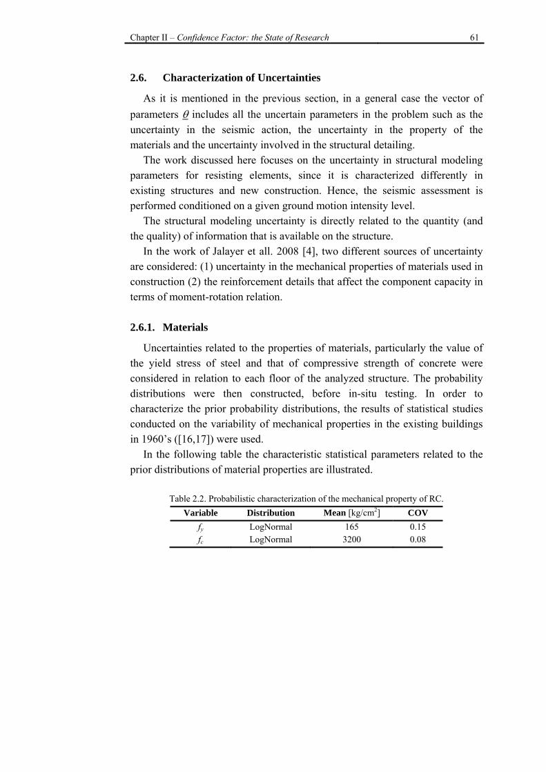
Chapter II – Confidence Factor: the State of Research 61
2.6. Characterization of Uncertainties
As it is mentioned in the previous section, in a general case the vector of parameters θ includes all the uncertain parameters in the problem such as the uncertainty in the seismic action, the uncertainty in the property of the materials and the uncertainty involved in the structural detailing.
The work discussed here focuses on the uncertainty in structural modeling parameters for resisting elements, since it is characterized differently in existing structures and new construction. Hence, the seismic assessment is performed conditioned on a given ground motion intensity level.
The structural modeling uncertainty is directly related to the quantity (and the quality) of information that is available on the structure.
In the work of Jalayer et all. 2008 [4], two different sources of uncertainty are considered: (1) uncertainty in the mechanical properties of materials used in construction (2) the reinforcement details that affect the component capacity in terms of moment-rotation relation. 2.6.1. Materials
Uncertainties related to the properties of materials, particularly the value of the yield stress of steel and that of compressive strength of concrete were considered in relation to each floor of the analyzed structure. The probability distributions were then constructed, before in-situ testing. In order to characterize the prior probability distributions, the results of statistical studies conducted on the variability of mechanical properties in the existing buildings in 1960’s ([16,17]) were used.
In the following table the characteristic statistical parameters related to the prior distributions of material properties are illustrated.
Table 2.2. Probabilistic characterization of the mechanical property of RC. Variable Distribution Mean [kg/cm2] COV
fy LogNormal 165 0.15 fc LogNormal 3200 0.08
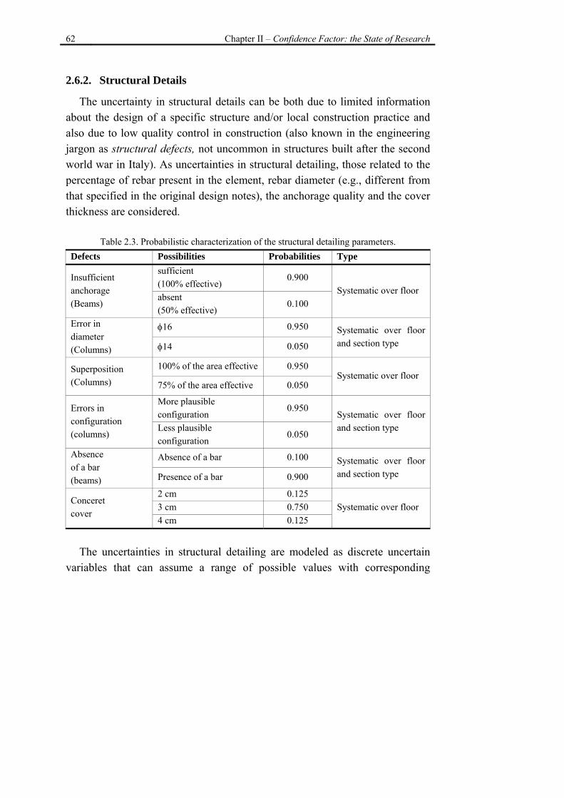
62 Chapter II – Confidence Factor: the State of Research
2.6.2. Structural Details
The uncertainty in structural details can be both due to limited information about the design of a specific structure and/or local construction practice and also due to low quality control in construction (also known in the engineering jargon as structural defects, not uncommon in structures built after the second world war in Italy). As uncertainties in structural detailing, those related to the percentage of rebar present in the element, rebar diameter (e.g., different from that specified in the original design notes), the anchorage quality and the cover thickness are considered.
Table 2.3. Probabilistic characterization of the structural detailing parameters. Defects Possibilities Probabilities Type
Insufficient anchorage (Beams)
sufficient (100% effective)
0.900 Systematic over floor
absent (50% effective)
0.100
Error in diameter (Columns)
φ16 0.950 Systematic over floor and section type φ14 0.050
Superposition (Columns)
100% of the area effective 0.950 Systematic over floor
75% of the area effective 0.050
Errors in configuration (columns)
More plausible configuration
0.950 Systematic over floor and section type Less plausible
configuration 0.050
Absence of a bar (beams)
Absence of a bar 0.100 Systematic over floor and section type Presence of a bar 0.900
Conceret cover
2 cm 0.125 Systematic over floor 3 cm 0.750
4 cm 0.125
The uncertainties in structural detailing are modeled as discrete uncertain
variables that can assume a range of possible values with corresponding
Chapter II – Confidence Factor: the State of Research 63
plausibilities/weights. In the absence of test results and in situ inspections, the a priori plausibility of each possible value is assigned qualitatively based on engineering consensus, judgment and experience.
It should be mentioned that once the test results are available on the quantity in question, they can be used applying the Bayesian methodology described in the previous sections to update the plausibility of each possible value for the corresponding discrete uncertain variable.
As it regards the correlation between different uncertain parameters, a simplified model of correlation is constructed by classifying different sets of correlated uncertain parameters within groups that are not cross-correlated [14]. 2.7. A Proposal for a Probabilistic Definition of Confidence Factor
Using the results of this work the authors have proposed a probability-based definition of the confidence factor.
In Figure 2.3 the histograms and the lognormal curves fitted for the demand to capacity ratio for three increasing levels of data considered in the work are shown. The first level corresponds to the prior lognormal probability distribution for the demand to capacity ratio before taking into consideration the test results. The second level corresponds to the updated distribution after considering the carrot test results for concrete and the tension test result for reinforcing steel. The last level illustrates the updated distribution for structural performance variable after considering also the ultrasonic test results for concrete.
For all three values of confidence level suggested by the code (i.e., CF=1,1.2,1.35) the corresponding demand to capacity ratios for the structure is calculated. The resulting three values for demand to capacity ratio are marked on the curves illustrated in Figure 2.3. Note that the failure threshold is also marked at the value of ln ln1.0 0.0Y = = .
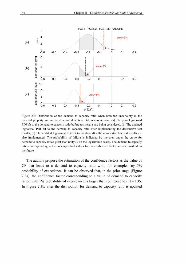
64 Chapter II – Confidence Factor: the State of Research
(a) -0.6 -0.5 -0.4 -0.3 -0.2 -0.1 0 0.1 0.2
0
2
4
6
prio
r
-0.6 -0.5 -0.4 -0.3 -0.2 -0.1 0 0.1 0.20
5
10
post
erio
r 1s
t le
vel
-0.6 -0.5 -0.4 -0.3 -0.2 -0.1 0 0.1 0.20
5
10
15
ln D/C
post
erio
r 2n
d le
vel
FC=1 FC=1.2 FC=1.35 FAILURE
area=5%
area=5%
area=5%
(b) (c)
Figure 2.3: Distribution of the demand to capacity ratio when both the uncertainty in the material property and in the structural defects are taken into account: (a) The prior lognormal PDF fit to the demand to capacity ratio before test results are being considered, (b) The updated lognormal PDF fit to the demand to capacity ratio after implementing the destructive test results, (c) The updated lognormal PDF fit to the data after the non-destructive test results are also implemented. The probability of failure is indicated by the area under the curve for demand to capacity ratios great than unity (0 on the logarithmic scale). The demand to capacity ratios corresponding to the code-specified values for the confidence factor are also marked on the figure.
The authors propose the estimation of the confidence factors as the value of CF that leads to a demand to capacity ratio with, for example, say 5% probability of exceedance. It can be observed that, in the prior stage (Figure 2.3a), the confidence factor corresponding to a value of demand to capacity ration with 5% probability of exceedance is larger than (but close to) CF=1.35. In Figure 2.3b, after the distribution for demand to capacity ratio is updated
Chapter II – Confidence Factor: the State of Research 65
after the destructive test results are considered, the demand to capacity ratio with 5% probability of exceedance corresponds to a confidence factor between CF=1.0 and CF=1.20. In Figure 2.3c, after the non-destructive test results are also considered, the demand to capacity ratio with 5% probability of exceedance corresponds to a confidence factor slightly greater than 1.0 which corresponds to the code-recommended value for the most complete level of knowledge. 3. Conclusions
In this chapter some interesting works which have addressed the open issues in the current code-based approach, obviously from different points of view, have been briefly discussed.
The present thesis work deals with the uncertainty in the assessment of existing RC buildings, analyzing the problem from the same point of view highlighted in the recent work of Jalayer et all, 2008 [4]. As in this chapter briefly presented and discussed, in this work the authors demonstrated that uncertainties in structural detailing can affect the structural reliability significantly. It was shown that considering the uncertainty in structural detailing parameters increases both the mean and standard deviation of the demand to capacity ratio for the structure. This finding, in the context of the code-based approach in which the confidence factors are applied to the mean material strength values only, emphasizes on the importance of calibrating them with respect to the global structural performance.
In order to characterize the uncertainties in the structural detailing parameters, prior probability mass functions are constructed based on all the information available excluding the test results. It was shown how a qualitative database of possible detailing parameters can be created by identifying the set of possibilities for each parameter and the corresponding plausibilities. This type of database, in lieu of test results and complete information about the structure, can be constructed based on both the qualitative judgment of the profession and also based on the construction practice at the time when the structure in question has been built.
66 Chapter II – Confidence Factor: the State of Research
The Bayesian updating algorithm implemented is general with respect to the type of in-situ test (e.g., also pseudo-dynamic test results can be implemented) performed and the standard error associated with it. Moreover, it allows for implementing the test data gradually and across increasing levels of knowledge with the goal of studying the changes in the updated representation of the structural performance. It was also demonstrated that the quality and quantity of the acquired test data significantly affects the updated (robust) reliability of the structure. It can observed that even a very small number of tests (e.g., only one in the case of steel resistance) can affect the distribution of demand to capacity ratio.
Moreover, defining the confidence factor as the value which leads to a demand to capacity ratio with a specified probability of being exceeded (e.g., 5%) in contrast to the code-specified values that are applied to mean values for material strength, has the advantage of measuring these factors in terms of the eventual structural performance instead of a modeling parameter. Nevertheless, for the case-study structure, the confidence factors, associated to each increasing level of knowledge, calculated based on the updated distribution of structural performance variable were consistent with the code-specified values.
Chapter II – Confidence Factor: the State of Research 67
4. References
[1] Monti G., Alessandri S., “Confidence factors for concrete and steel strength”, Convegno RELUIS “Valutazione e riduzione della vulnerabilità sismica di edifici esistenti in cemento armato”, Roma 29-30 maggio 2008.
[2] Franchin P., Pinto P. E., Pathmanathan R., “Confidence in confidence factor”, Convegno Finale RELUIS – REte Laboratori Universitari Ingegneria Sismica, Napoli, Italia, 1-3aprile 2009.
[3] Jalayer F., Iervolino I., Manfredi G., “Influenza dei parametri di modellazione e dell’incertezza associata nella valutazione sismica di edifici esistenti in cemento armato”, Proceedings XII Convegno ANIDIS, Giugno 2007.
[4] Jalayer F., Iervolino I., Manfredi G., “Structural modeling uncertainties and their influence on seismic assessment of existing RC structures”, submitted to Structural Safety, 2008.
[5] Fajfar, P. “Capacity spectrum method based on inelastic demand spectra”, Earthquake Engineering and Structural Dynamics; 28:979–93, 1999.
[6] Ordinanza del Presidente del Consiglio dei Ministri (OPCM) n. 3431, Ulteriori modifiche ed integrazioni all'ordinanza del Presidente del Consiglio dei Ministri n. 3274 del 20 marzo 2003. Gazzetta Ufficiale della Repubblica Italiana n. 107 del 10-5-2005 (Suppl. Ordinario n.85), 2005.
[7] Ordinanza del Presidente del Consiglio dei Ministri (OPCM) n. 3519. Criteri per l’individuazione delle zone sismiche e la formazione e l’aggiornamento degli elenchi delle medesime zone. Gazzetta Ufficiale della Repubblica Italiana n. 108, 2006.
[8] Regio Decreto Legge (R.D.L.) 2229. Norme per l’esecuzione delle opere in conglomerato cementizio semplice o armato, 1939.
[9] Mander J.B., Priestley M.J.N., Park R., Theoretical stress-strain model for confined concrete, Journal of Structural Engineering, vol.114, n.8, August 1988, pp.1804-1826.
[10] Beck, J.L., Katafigiotis, L.S. “Updating models and their uncertainties. I: Bayesian statistical framework”, Journal of Engineering Mechanics, Vol. 124, no. 4, April 1998.
[11] Beck J.L., Au S.K., “Bayesian updating of structural models and reliability using Markov chain Monte Carlo simulation”, Journal of Engineering Mechanics, Vol.128, no. 4, April 2002.

68 Chapter II – Confidence Factor: the State of Research
[12] Hastings, W.K. Monte-Carlo sampling methods using Markov Chains and their applications. Biometrika; 57(1), 97-109, 1970.
[13] Au S.K., Beck J.L. First excursion probabilities for linear systems by very efficient importance sampling. Probabilistic Engineering Mechanics; Vol. 16:193-207, 2001.
[14] Au, S.K., Beck, J.L. “Subset simulation and its application to probabilistic seismic performance assessment”, Journal of Engineering Mechanics, Vol. 16, no. 4, 2003.
[15] Jalayer, F., Franchin, P. and Pinto, P.E. “A Scalar Decision Variable for Seismic Reliability Analysis of RC Frames”, Earthquake Engineering and Structural Dynamics Special Issue on Structural Reliability, Vol. 36 (13): 2050-2079, 2007a.
[16] Verderame, G.M., Manfredi, G., Frunzio G., “Le proprietà meccaniche dei calcestruzzi impiegati nelle strutture in cemento armato realizzate negli anni ’60”, X Congresso Nazionale “L’ingegneria Sismica in Italia”, Potenza-Matera 9-13 settembre 2001a.
[17] Verderame, G.M., Stella, A., Cosenza, E., “Le proprietà meccaniche degli acciai impiegati nelle strutture in cemento armato realizzate negli anni ’60”, X Convegno Nazionale "L'Ingegneria Sismica in Italia", Potenza e Matera 9-13 Settembre 2001b.
69 Chapter III – Uncertainty in the Representation of Ground Motion
Chapter III
Uncertainty in the Representation of Ground Motion
1. Introduction
The uncertainty in the representation of ground motion is strictly related to the selection of the ground motion records to be used in the structural assessment employing dynamic analysis.
The seismic input selection represents one of the main issues in assessing the seismic response of a structure through numerical dynamic analysis. In some cases the records are selected to have response spectra that approximate the uniform hazard spectrum or other “design” response spectrum (e.g., [1, 2]). In general, it is reasonable to choose ground motion records whose magnitude, distance, site conditions and mechanisms of fault are representative for the seismic hazard at the site of the structure under consideration. This choice may be guided by the disaggregation of the seismic hazard [3] for the site of interest. However, once the set of records is chosen, there are several techniques to evaluate the structural seismic response [4].
In the framework of PBEE (chapter II), the choice of the ground motions may be affected by the interface variable used to measure the intensity of ground motion, known as the intensity measure IM.
70 Chapter III – Uncertainty in the Representation of Ground Motion
According to criteria proposed by Luco and Cornell [5] a preferred IM is both “sufficient” with respect to the ground motion characteristics and also “efficient”. A sufficient IM renders the structural response conditionally statistically independent of other ground motion characteristics such as event magnitude, while an efficient IM predicts the structural response with (relatively) small record-to-record variability.
Theoretically, careful record selection is not essential if the IM is demonstrated to be sufficient with respect to ground motion characteristics [6]. It has to be recalled that sufficiency of a specific IM depends on the structure, the structural response parameters and the ground motion characteristics. Ground motion parameters such as site amplification and/or directivity may prove particularly troublesome because they may imply strong sensitivity of spectral shape to certain ground motion parameters [7].
A useful strategy, in cases where the adopted scalar intensity measure IM1 does not prove to be sufficient, is to introduce an additional intensity measure, IM2. That is, one can adopt a vector-valued intensity measure IM=[IM1,IM2], consisting of two scalar IM’s, in order to render a more complete description of the ground motion characteristics [8]. 2. Ground Motion Record Selection
In this chapter, an approximate method based on linear regression is used in order to establish possible correlation between the structural response conditional on the primary intensity measure IM1 and the secondary intensity measure IM2. Moreover, a weighting scheme based on seismic hazard disaggregation is used, in the framework of the scalar intensity measure IM1, in order to adjust the structural response for possible correlations with a candidate secondary intensity measure. This weighting scheme can be implemented in non-linear dynamic analysis procedure both for a wide range of ground motion intensities and also for a limited range of ground motion intensities.
The efficiency of the weighting scheme is evaluated in terms of seismic risk which is represented herein by the mean annual frequency (MAF) of exceeding the critical component demand to capacity ratio. The seismic risk curves are
Chapter III – Uncertainty in the Representation of Ground Motion 71
obtained related to the adoption of both scalar and vector-valued intensity measures.
The chapter begins by an overview of the procedure for probabilistic performance assessment of buildings based on both scalar and vector ground motion intensity measures. Then the structural model chosen as the case-study and the ground motion record selections used for non-linear dynamic analysis are presented. In subsequent sections the IM’s studied in this work for predicting structural response and the structural engineering parameter used to measure the global performance of the structure are introduced. It is demonstrated how site-specific seismic hazard disaggregation can be used in order to obtain the conditional probability distribution for the secondary IM given the primary IM. Moreover, the application of the so-called residual-residual plots in establishing sufficiency of the adopted IM is discussed.
Distinguished by the amount of structural analysis required, two alternative non-linear dynamic analysis procedures, namely the cloud and the stripe method are introduced. The weighted cloud and the weighted stripes methods are then introduced as analysis procedures which manipulate the structural response to the selected ground motion records by employing the information provided from the seismic hazard analysis. Finally, the mean annual frequency of exceeding a global structural performance variable is used in order to benchmark the candidate intensity measures for the case-study structure. 3. Probabilistic Assessment based on Non-Linear Dynamic Analysis
As discussed in chapter II, a probabilistic performance-based criterion for seismic assessment of existing structures can be written as:
0PDM ≤λ Eq.3.1
72 Chapter III – Uncertainty in the Representation of Ground Motion
where λDM refers to the MAF of exceeding a specified damage level3 and P0 is the allowable probability threshold for the assessment4.
In order to calculate λDM using non-linear time-history analyses, it is common to use an intermediate parameter known as the IM in order to relate the characteristics ground motion record to the structural performance. The annual rate of exceeding a specified limit state can be expanded, using the principles of probability theory, with respect to the adopted (scalar) IM in the following:
∫ >= )()()( xdxyDMPy IMIMDMDM λλ Eq.3.2
The first term in the integrand PDM|IM(DM > y|x) is the conditional
probability of exceeding the damage threshold y for a given value of the IM=x. This term is also known as the structural fragility. The second term in the integrand is the absolute value of the derivative of the annual rate of exceeding IM=x; this second term is known as the hazard for the adopted IM. Ideally, the hazard function for the adopted IM is obtained from the results of site-specific probabilistic seismic hazard analysis (PSHA, see [9]).
The non-linear dynamic analysis procedures based on a limited suite of ground motion records can be used to estimate the fragility term in the integrand in equation 3.2. Depending on the amount of structural analysis and also on the range of limit states for which the performance assessment is done, two alternative non-linear dynamic analysis procedures are considered in this work, the cloud method and the stripes method [10, 4, 11].
3 It is desirable to express the performance objectives in terms of life-cycle cost [9]. However, the focus of this work is on ground motion record selection for the purpose of estimating non-linear structural response. Therefore, the performance objective is hereby stated in terms of a structural damage index instead of economic indices. 4 Note that in equation 3.1 it has been assumed that the numerical value for rate of exceedance is close to that of the probability of exceedance; this is true for small values of the exceedance probability representing very rare events.
Chapter III – Uncertainty in the Representation of Ground Motion 73
The cloud method employs the linear least squares scheme to the specified DM based on non-linear structural response (cloud response) for a suite of ground motion records (un-scaled) in order to estimate the conditional mean and standard deviation of DM given IM. A linear relationship (determined using regression) between the logarithms of the two variables provides a reasonable estimate of the mean value of the logarithm of DM. Moreover, by assuming that the errors of the least square estimate are independent and identically distributed (i.i.d.), and assuming a Gaussian distribution for the logarithm of DM given IM), the PDM|IM(DM > y|x) can be estimated using the Complementary Cumulative Distribution Function (CCDF):
⎟⎟⎠
⎞⎜⎜⎝
⎛ −Φ−==>
)(ln)(lnln
1)()(xy
xyyxyGxyDMP IMDMIMDM σ
η Eq.3.3
where η(ln y|x) and σ(ln y|x) are the conditional mean and standard deviation of the logarithm of DM given a specific IM level respectively.
Alternatively, the stripes method provides the non-linear structural response parameters for the suite of records that are scaled to successively increasing IM levels: this is referred to as the stripe response. Subsequently, the statistical properties of the stripe responses for various IM levels, calculated based on the response to the suite of records, can be employed to obtain the probability of exceeding a specified damage level.
In the case where a vector-valued IM=[IM1,IM2] consisting of two scalar IM’s is adopted, the fragility term in equation 3.2 for the annual rate of exceeding DM=y can be expanded with respect to IM2 and re-arranged as following:
)()(),()(11212 , xdxzfzxyDMPy IMIMIMIMIMDMDM λλ ∫∫ >= Eq.3.4
74 Chapter III – Uncertainty in the Representation of Ground Motion
The first term in the integrand is the conditional probability of exceeding DM=y given IM1 and IM2 and the second term is the conditional probability density function (PDF) for IM2=z given IM1=x. Similar to the case regarding scalar IM, both cloud method and stripes method can be employed in order to perform probabilistic seismic risk assessments. In the context of cloud method, the two-variable linear least squares scheme can be used to estimate the statistical parameters for the damage measure conditional on both IM1 and IM2. Also in this case, by assuming that the errors of the multiple linear least square estimate are independent and identically distributed (i.i.d.), and assuming a Gaussian distribution for the logarithm of DM given IM1 and IM2, the
),(21 , zxyDMP IMIMDM > can be estimated using the Complementary
Cumulative Distribution Function (CCDF):
=> ),(21 , zxyDMP IMIMDM
⎟⎟⎠
⎞⎜⎜⎝
⎛
σ
η−Φ−==
),(ln),(lnln
1),(21 , zxy
zxyyzxyG IMIMDM
Eq.3.5
where η(ln y|x,z) and σ(ln y|x,z) are the conditional mean and standard deviation of the logarithm of DM given IM1=x and IM2=z. Alternatively, using the stripes methods, the simple linear least squares can be applied to the stripe response at various IM1 level with IM2 as the independent variable. 3.1. The Intensity Measures for Predicting Structural Response
The IMs can be considered either as a scalar or a vector of parameters that are proxies for the ground motion potential with respect to structural response. In this chapter, both scalar and vector IM’s are studied.
As scalar IM’s, the peak ground acceleration (PGA) and the spectral acceleration at the first mode denoted as Sa(T1) are considered. As vector IM’s, the pairs consisting of PGA and magnitude M, Sa(T1) and the deviation from the ground motion prediction model, ε, are considered. Furthermore, the pair
Chapter III – Uncertainty in the Representation of Ground Motion 75
consisting of Sa(T1) and the spectral acceleration at a period T2 ≠ T1, (Sa(T2)) is considered. In particular, as will be explained later, T2 is the second period whose spectral acceleration is most efficient in predicting structural response.
PGA has been widely used as the ground motion IM in the past. Recently, Sa(T1) is considered and verified to be a more suitable choice of an IM, as it reflects the elastic response of a single degree of freedom (SDOF) system with a period equal to the first-mode period of the structure and hazard curves are also available for this IM. However, it is unable to reflect the effect of higher frequencies (higher modes in a structure with several degrees of freedom) or lower frequencies (severe non-linear behavior in the structural elements) or the near-source effects (a single low frequency pulse dominating the ground motion record).
Ideally, one should use a vector consisting of Sa(T1) and an IM related to the spectral shape, for example the ratio R(T) = Sa(T)/ Sa(T1) [12], where T is the second period whose spectral value is considered as important to the structural response. It has been also demonstrated that epsilon may act as a proxy for the spectral shape [8]. 3.2. The Structural Engineering Parameters
The structural engineering parameter used in this work, to measure the global performance of the structure subjected to seismic excitation, is the critical demand to capacity ratio.
It is desirable to express the performance objective in terms of a (scalar) system damage measure which reflects how far away the structure is from the threshold of the limit state [13], namely:
01 PDVLS ≤= >λλ Eq.3.6
The decision variable can be defined as the ratio of system demand D to
system capacity CLS, (e.g., ratio of θmax to θCLS) or it can be defined as a functional of component demand and capacities, which is equal to one at the
76 Chapter III – Uncertainty in the Representation of Ground Motion
onset of failure. This latter formulation is the one adopted in this work. In this work the scalar system decision variable, denoted by Y, is defined as the demand to capacity ratio of the critical component, i.e., that component that brings the system closest to failure:
1 1max minmech l jlN Nl j
jl
DY
C= == Eq.3.7
where Nmech is the number of considered potential failure mechanisms and Nl is the number of components taking part in the lth mechanism. This corresponds to the system reliability concept of cut-set [14], defined as any set of components whose joint failure, jljl
ljl CDY 1min == , implies the failure of the system,
lNl YY mech
1max == .
4. The Case-Study Structure
The case study structure analyzed is the same considered in the previous chapter that is an existing RC school building in the city of Avellino.
In order to employ non-linear dynamic analysis both for a limited and a wide range of value of the IM, the finite element model of the central frame of the structure is constructed using the Open System for Earthquake Engineering Simulation (OpenSees) software. In particular the force-based beam with hinges model [15] has been employed assuming that the non-linear behavior in the structure is concentrated in plastic hinges located at the element ends (Appendix A). This type of element consists of three parts. Two hinges at the ends characterized as rigid plastic elements, and a linear-elastic region in the middle. The stiffness of the rigid-plastic element is defined by its moment-rotation relation which is derived by analyzing the reinforced concrete section at the hinge location. In this study, the section analysis is based on the Mander-Priestly [16] constitutive relation for reinforced concrete assuming that the concrete is not confined and the reinforcing steel behavior is elastic-plastic.
Chapter III – Uncertainty in the Representation of Ground Motion 77
As mentioned in the previous chapter the behavior of the plastic hinge is characterized by four phases, namely: rigid phase, cracked phase, post-yielding phase and post-peak phase. In addition to flexural deformation, the yielding rotation takes into account also the shear deformation and the deformation related to bar slip based on the code recommendations [17] (Appendix B). Moreover, the shear span used in the calculation of the plastic rotation is based on the code formulas. As it regards the post-peak behavior, it is assumed that the section resistance drops to zero, resulting in a tri-linear curve.
The length of the two hinges at the ends is approximated by the semi-empirical formulas provided for the plastic hinge length in the Italian code [17] which take into account both the effect of shear and bar slip in the (post peak) ultimate phase of the section behavior. The plastic hinges take into account the superposition of both flexural and axial action. The axial action models, in parallel, the reinforcing steel as elastic-perfectly plastic and concrete as elastic-no tension. In order to model the flexural action in the hinges, the moment-curvature curves calculated for the plastic hinges described above are utilized. The structural damping is modeled based on the Rayleigh model and is assumed to be equal to 5% for the first two modes. The small amplitude period for the first two vibration modes are equal to 0.73 and 0.26 seconds respectively. 5. The Suites of Ground Motion Records and their Properties
Two different suites, respectively of 21 (Sel_A) and 20 (Sel_B) ground motion records, have been selected for this study. They are all main-shock recordings recorded on stiff soil (400 m/s < Vs30 < 700 m/s) which is consistent with the soil-type for the site. The first suite of records has been chosen in order to cover a wide range of moment magnitude values; for the second suite of records the same goal has been pursued in terms of the deviation from the ground motion prediction model epsilon.
Epsilon is defined as the number of standard deviations by which an observed logarithmic spectral acceleration differs from the mean logarithmic spectral acceleration of a ground-motion prediction (attenuation) equation. The

78 Chapter III – Uncertainty in the Representation of Ground Motion
equation corresponding to this definition is:
)(ln
)(ln
ˆˆ)(ln
TS
TSa
a
aTSσ
µε
−= Eq.3.8
where ln Sa(T) is the natural logarithm of the spectral acceleration value of the record at a specified period T, and )(lnˆ TSa
µ and )(lnˆ TSaσ are the estimate mean
and standard deviation as predicted by an attenuation equation. The definition of ε is valid for any ground motion prediction model, but the model of Sabetta and Pugliese [18] is the only one used in calculations here. It should be noted that epsilon is defined with respect to the unscaled record and will not change in value when the record is scaled. 4.1. Record Selection A (Sel_A)
The first suite is based on Mediterranean events taken from European Strong-Motion Database or ESD5 (17 recordings) and Pacific Earthquake Engineering Research Next Generation Attenuation of Ground Motions or PEER NGA6 Database (4 recordings). The earthquake events have moment magnitude (Mw) between 5.3 and 7.2, and closest distances ranging between 7km and 30km. Table 3.1 illustrates the ground motion recordings, their Mw, the fault mechanism (FM), the velocity of propagations of the shear waves (Vs30, symbol “?” indicates that the value is not available), epicentral distance (ED), fault distance (FD), peak ground acceleration (PGA), spectral acceleration at the first mode (Sa(T1)) and ε values for each record.
5 http://www.isesd.cv.ic.ac.uk/ESD/Database/Database.htm 6http://peer.berkeley.edu/nga/flatfile.html
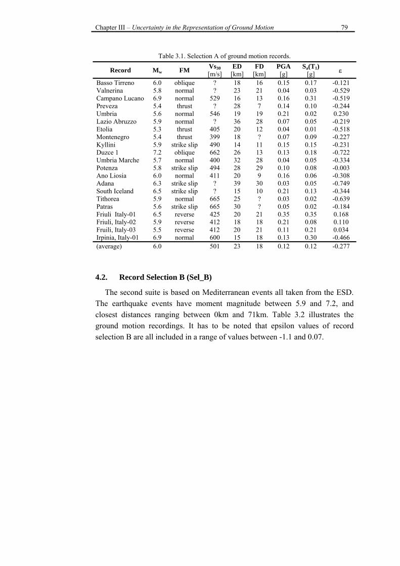
Chapter III – Uncertainty in the Representation of Ground Motion 79
Table 3.1. Selection A of ground motion records.
Record Mw FM Vs30 [m/s]
ED [km]
FD [km]
PGA [g]
Sa(T1) [g] ε
Basso Tirreno 6.0 oblique ? 18 16 0.15 0.17 -0.121 Valnerina 5.8 normal ? 23 21 0.04 0.03 -0.529 Campano Lucano 6.9 normal 529 16 13 0.16 0.31 -0.519 Preveza 5.4 thrust ? 28 7 0.14 0.10 -0.244 Umbria 5.6 normal 546 19 19 0.21 0.02 0.230 Lazio Abruzzo 5.9 normal ? 36 28 0.07 0.05 -0.219 Etolia 5.3 thrust 405 20 12 0.04 0.01 -0.518 Montenegro 5.4 thrust 399 18 ? 0.07 0.09 -0.227 Kyllini 5.9 strike slip 490 14 11 0.15 0.15 -0.231 Duzce 1 7.2 oblique 662 26 13 0.13 0.18 -0.722 Umbria Marche 5.7 normal 400 32 28 0.04 0.05 -0.334 Potenza 5.8 strike slip 494 28 29 0.10 0.08 -0.003 Ano Liosia 6.0 normal 411 20 9 0.16 0.06 -0.308 Adana 6.3 strike slip ? 39 30 0.03 0.05 -0.749 South Iceland 6.5 strike slip ? 15 10 0.21 0.13 -0.344 Tithorea 5.9 normal 665 25 ? 0.03 0.02 -0.639 Patras 5.6 strike slip 665 30 ? 0.05 0.02 -0.184 Friuli Italy-01 6.5 reverse 425 20 21 0.35 0.35 0.168 Friuli, Italy-02 5.9 reverse 412 18 18 0.21 0.08 0.110 Fruili, Italy-03 5.5 reverse 412 20 21 0.11 0.21 0.034 Irpinia, Italy-01 6.9 normal 600 15 18 0.13 0.30 -0.466 (average) 6.0 501 23 18 0.12 0.12 -0.277 4.2. Record Selection B (Sel_B)
The second suite is based on Mediterranean events all taken from the ESD. The earthquake events have moment magnitude between 5.9 and 7.2, and closest distances ranging between 0km and 71km. Table 3.2 illustrates the ground motion recordings. It has to be noted that epsilon values of record selection B are all included in a range of values between -1.1 and 0.07.
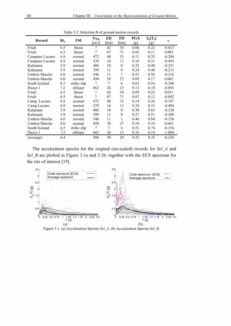
80 Chapter III – Uncertainty in the Representation of Ground Motion
Table 3.2. Selection B of ground motion records.
Record Mw FM Vs30 [m/s]
ED [km]
FD [km]
PGA [g]
Sa(T1) [g] ε
Friuli 6.5 thrust ? 42 34 0.06 0.22 -0.015 Friuli 6.5 thrust ? 87 71 0.05 0.11 0.003 Campano Lucano 6.9 normal 472 48 33 0.11 0.25 -0.204 Campano Lucano 6.9 normal 529 16 13 0.16 0.31 -0.493 Kalamata 5.9 normal 486 10 0 0.22 0.48 -0.231 Kalamata 5.9 normal 399 11 0 0.24 0.48 -0.233 Umbria Marche 6.0 normal 546 11 1 0.52 0.56 -0.216 Umbria Marche 6.0 normal 450 38 27 0.09 0.17 0.062 South Iceland 6.5 strike slip ? 7 6 0.63 0.54 -0.288 Duzce 1 7.2 oblique 662 26 13 0.13 0.18 -0.893 Friuli 6.5 thrust ? 42 34 0.09 0.25 0.031 Friuli 6.5 thrust ? 87 71 0.07 0.12 -0.002 Camp. Lucano 6.9 normal 472 48 33 0.14 0.26 -0.187 Camp.Lucano 6.9 normal 529 16 13 0.18 0.31 -0.484 Kalamata 5.9 normal 486 10 0 0.30 0.63 -0.120 Kalamata 5.9 normal 399 11 0 0.27 0.51 -0.208 Umbria Marche 6.0 normal 546 11 1 0.46 0.64 -0.156 Umbria Marche 6.0 normal 450 38 27 0.10 0.18 0.065 South Iceland 6.5 strike slip ? 7 6 0.51 0.74 -0.154 Duzce 1 7.2 oblique 662 26 13 0.16 0.14 -1.004 (average) 6.4 506 30 20 0.22 0.35 -0.236
The acceleration spectra for the original (un-scaled) records for Sel_A and Sel_B are plotted in Figure 3.1a and 3.1b, together with the EC8 spectrum for the site of interest [19].
(a) (b)
Figure 3.1. (a) Acceleration Spectra Sel_A. (b) Acceleration Spectra Sel_B.
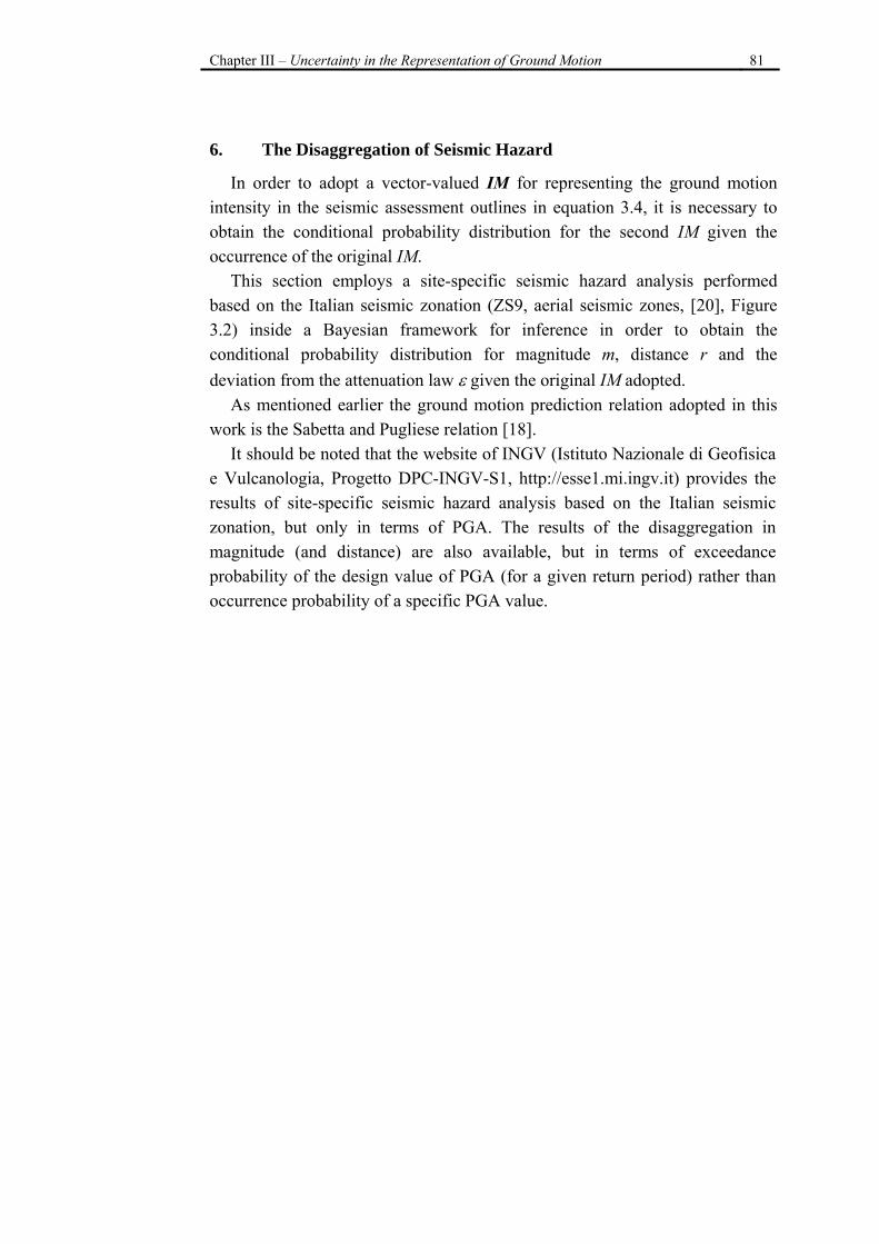
Chapter III – Uncertainty in the Representation of Ground Motion 81
6. The Disaggregation of Seismic Hazard
In order to adopt a vector-valued IM for representing the ground motion intensity in the seismic assessment outlines in equation 3.4, it is necessary to obtain the conditional probability distribution for the second IM given the occurrence of the original IM.
This section employs a site-specific seismic hazard analysis performed based on the Italian seismic zonation (ZS9, aerial seismic zones, [20], Figure 3.2) inside a Bayesian framework for inference in order to obtain the conditional probability distribution for magnitude m, distance r and the deviation from the attenuation law ε given the original IM adopted.
As mentioned earlier the ground motion prediction relation adopted in this work is the Sabetta and Pugliese relation [18].
It should be noted that the website of INGV (Istituto Nazionale di Geofisica e Vulcanologia, Progetto DPC-INGV-S1, http://esse1.mi.ingv.it) provides the results of site-specific seismic hazard analysis based on the Italian seismic zonation, but only in terms of PGA. The results of the disaggregation in magnitude (and distance) are also available, but in terms of exceedance probability of the design value of PGA (for a given return period) rather than occurrence probability of a specific PGA value.
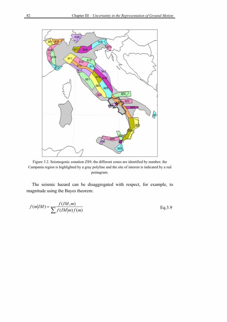
82 Chapter III – Uncertainty in the Representation of Ground Motion
Figure 3.2. Seismogenic zonation ZS9; the different zones are identified by number; the
Campania region is highlighted by a gray polyline and the site of interest is indicated by a red pentagram.
The seismic hazard can be disaggregated with respect, for example, to
magnitude using the Bayes theorem:
∑=
)()(),()(
mfmIMfmIMfIMmf Eq.3.9
Chapter III – Uncertainty in the Representation of Ground Motion 83
Supposing that the site of interest is surrounded by aerial seismic zones, and using the total probability theorem, the term f(IM,m) can be further expanded with respect to the seismo-genetic areas surrounding the site and the distance r of the points within each area to the site of interest:
)(
)()()(),,()(
IMp
frfmfrmIMIIMmf i R
i∑∑∑= ε
εεα Eq.3.10
where αi is the relative seismicity of seismic area Ai with respect to other
seismic zones considered (αi=λi/Σλ, where λi is the seismicity of zone i). The term Ι(IM | m, r, ε) is an indicator function reflecting the fact that given the epsilon, distance and magnitude, the IM value is going to be known deterministically from the ground motion prediction relationship. That is Ι(IM | m, r, ε) can assume only two values, namely, zero and unity. It should be noted that, given that an earthquake takes place in seismic zone Ai, it is assumed that it is equally likely to have its epicenter located anywhere inside the area. Therefore, the probability f(r) of having an earthquake with its epicenter inside the areal increment dA, whose center is individuated by the distance r, can be calculated as dA/A where A is the total area of the seismic zone.
The probability density function (PDF) for the magnitude can be calculated from the Gutenberg-Richter truncated distribution:
ul mm
m
eeemf ⋅−⋅−
⋅−
−⋅
= ββ
ββ)( Eq.3.11
where β is the Richter b-value times ln(10) and ml and mu are a lower and an upper bound magnitude, respectively.
Table 3.3 illustrates the seismicity λ, the Richter b-value and a lower and upper magnitude bound (ml and mu, respectively) for those ZS9 seismic zones surrounding the Campania region.
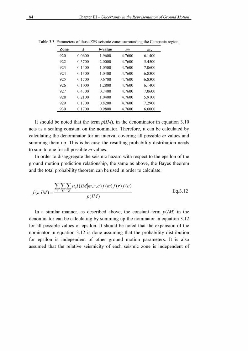
84 Chapter III – Uncertainty in the Representation of Ground Motion
Table 3.3. Parameters of those ZS9 seismic zones surrounding the Campania region.
Zone λ b-value ml mu 920 0.0600 1.9600 4.7600 6.1400 922 0.3700 2.0000 4.7600 5.4500 923 0.1400 1.0500 4.7600 7.0600 924 0.1300 1.0400 4.7600 6.8300 925 0.1700 0.6700 4.7600 6.8300 926 0.1000 1.2800 4.7600 6.1400 927 0.4300 0.7400 4.7600 7.0600 928 0.2100 1.0400 4.7600 5.9100 929 0.1700 0.8200 4.7600 7.2900 930 0.1700 0.9800 4.7600 6.6000
It should be noted that the term p(IM), in the denominator in equation 3.10
acts as a scaling constant on the nominator. Therefore, it can be calculated by calculating the denominator for an interval covering all possible m values and summing them up. This is because the resulting probability distribution needs to sum to one for all possible m values.
In order to disaggregate the seismic hazard with respect to the epsilon of the ground motion prediction relationship, the same as above, the Bayes theorem and the total probability theorem can be used in order to calculate:
)(
)()()(),,()(
IMp
frfmfrmIMIIMf i M R
i∑∑∑=
εεαε Eq.3.12
In a similar manner, as described above, the constant term p(IM) in the
denominator can be calculating by summing up the nominator in equation 3.12 for all possible values of epsilon. It should be noted that the expansion of the nominator in equation 3.12 is done assuming that the probability distribution for epsilon is independent of other ground motion parameters. It is also assumed that the relative seismicity of each seismic zone is independent of
Chapter III – Uncertainty in the Representation of Ground Motion 85
other parameters. Moreover, it is assumed that the probability distribution for magnitude is the same for all the points within a given seismic area.
The conditional probability distributions of magnitude given peak ground acceleration and of epsilon of the prediction law given the spectral acceleration at first mode, have been obtained through the disaggregation of the seismic hazard for the site of the case study structure using the Bayesian framework here described.
Figure 3.3. (a) Conditional probability distribution of M given some values of PGA and
histogram of M values for Sel_A. (b) Conditional probability distribution of ε given some values of Sa(T1) and histogram of ε values for Sel_B.
The distributions f(m|PGA) obtained for increasing levels of PGA are
illustrated in Figure 3.3a; moreover, the histogram of the values of magnitude of the record selection A is also shown in the bottom of the figure. In the same manner, the distributions f(ε|Sa(T1))) obtained for increasing levels of Sa(T1) are illustrated in Figure 3.3b; the histogram of the values of epsilon of the record selection B is also plotted in the bottom of the figure.
7. Residual – Residual Plot
Linear regression is a useful statistical tool for investigating efficiency and sufficiency criteria for a candidate IM (see [21, 22]). The damage measure, Y,
86 Chapter III – Uncertainty in the Representation of Ground Motion
can be predicated as a function of the candidate IM, e.g., PGA or Sa(T1), by performing linear regression (usually in the logarithmic scale). The efficiency of the candidate IM can be measured by the variability in the residuals of the regression analysis. In order to establish sufficiency, the effectiveness of ground motion characteristic variables as additional regression variables (i.e., in addition to IM1) can be investigated. In other words, ground motion characteristic variables cause very little improvement in the regression prediction as regression variables in addition to a “sufficient” IM. This improvement may be judged by the reduction in the dispersion of the regression residuals and/or the statistical significance of the regression coefficients corresponding to the ground motion characteristic variables.
In this study, a simplified statistical approach based on regression is implemented for measuring the effectiveness of ground motion characteristics as additional regression variables. This method uses a graphical statistical tool known as the residual-residual plot. The main advantage of the residual-residual plots is that they offer visual means for judging the improvement caused by an additional regression variable.
Residual-residual plots are used in the applied statistics in order to investigate whether adding a second variable to the regression improves the predictions compared to predictions based on the regression on the first variable only. These plots are constructed by: a) performing regression of the dependent variable (e.g., the damage measure, Y) versus the (first) independent variable IM1 (e.g., PGA or Sa(T1)) b) performing regression of the second independent variable IM2 (e.g., one of the ground motion characteristics) on also the first variable IM1 c) plotting the residuals of the two regressions mentioned above against each other.
Roughly speaking, the two regressions on the first variable “eliminate” possible dependence of both the dependent variable (Y) and the second independent variable (one of the ground motion characteristics) on the first independent variable (PGA or Sa(T1)). This facilitates investigating the potential dependence of the dependent variable on the second variable, by observing a (statistically) significant trend, in the residual-residual plot,
Chapter III – Uncertainty in the Representation of Ground Motion 87
between the two sets of residuals explained above. In order to simplify future references to these residuals, the residuals of the regression of the dependent variable on the first variable are also called the “response residuals”, and the residual of the regression of the second variable on the first variable are also called the “second-variable residuals”. The possible trend between the two sets of residuals may be observed by performing linear regression of “response residuals” on “second variable residuals”. The significance of the trend measured by both the variability in the residuals of such regression and/or testing the following hypothesis: “The slope of the regression line is zero” (i.e., test of hypothesis). The significance of the slope is usually measured by a quantity known as the p-value, assuming that the slope of the regression line is a random variable described by Student’s T-distribution (see [23]). The hypothesis is rejected (i.e., the slope is non-zero) if the p-value is smaller than a certain (small) value, e.g., 0.01. If a two-variable regression of the response on both the first and the second independent variable is performed, it can be shown that the regression coefficient for the second variable is going to be the same as the slope of the (simple) regression of the “response residuals” on “second-variable residuals”. Moreover, the results of the hypothesis test are going to be identical.
As it is mentioned above, one way to measure the significance of an additional regression variable is by measuring the amount of reduction it causes in the variability of data around the regression prediction. The variability of data around the regression line can be estimated by the (square) root of the mean of squares (RMS) of regression residuals, which is also referred to as the “sigma” of the regression. It should be noted that the “sigma” of the residual-residual regression is the same as that of the two-variable regression of response (dependent variable) on the two independent variables, i.e., the two approaches are equivalent. The smaller is the ratio of the sigma of the residual-residual regression (explained above) to the sigma of the regression of dependent variable on the first variable (or “original” regression for brevity), the more significant is the role of the second regression variable. In simple terms, an effective second regression variable is going to “explain” part of the
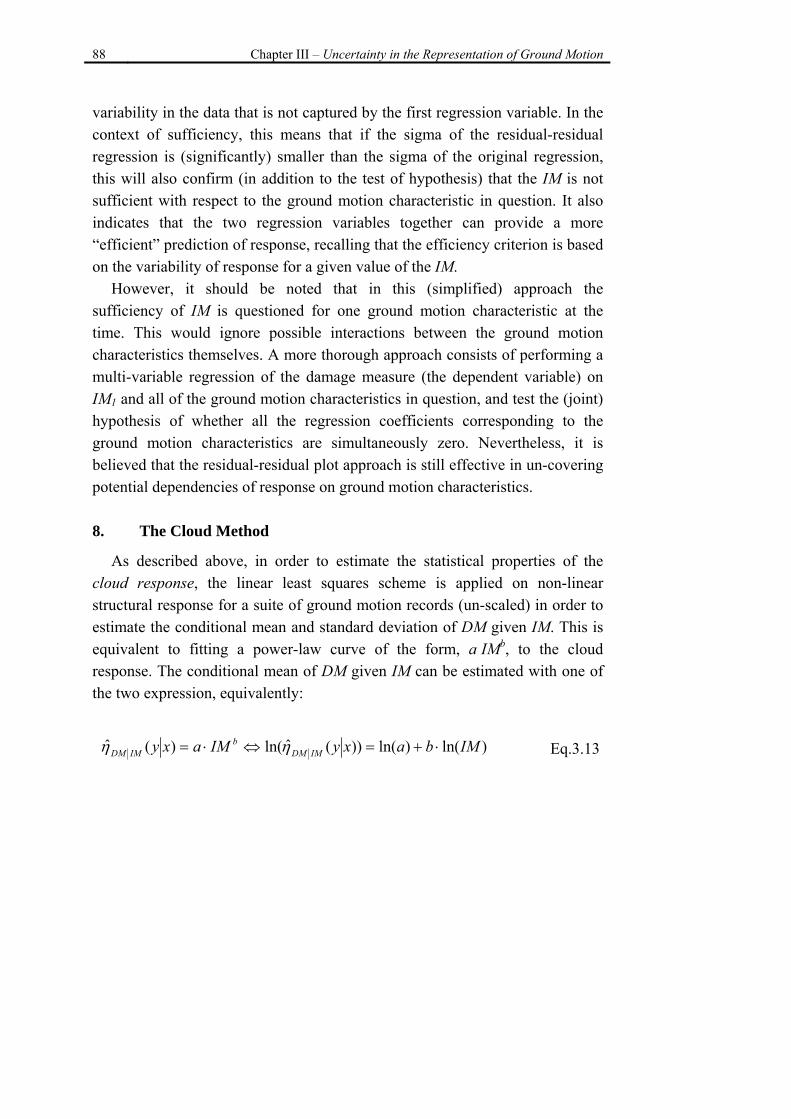
88 Chapter III – Uncertainty in the Representation of Ground Motion
variability in the data that is not captured by the first regression variable. In the context of sufficiency, this means that if the sigma of the residual-residual regression is (significantly) smaller than the sigma of the original regression, this will also confirm (in addition to the test of hypothesis) that the IM is not sufficient with respect to the ground motion characteristic in question. It also indicates that the two regression variables together can provide a more “efficient” prediction of response, recalling that the efficiency criterion is based on the variability of response for a given value of the IM.
However, it should be noted that in this (simplified) approach the sufficiency of IM is questioned for one ground motion characteristic at the time. This would ignore possible interactions between the ground motion characteristics themselves. A more thorough approach consists of performing a multi-variable regression of the damage measure (the dependent variable) on IM1 and all of the ground motion characteristics in question, and test the (joint) hypothesis of whether all the regression coefficients corresponding to the ground motion characteristics are simultaneously zero. Nevertheless, it is believed that the residual-residual plot approach is still effective in un-covering potential dependencies of response on ground motion characteristics. 8. The Cloud Method
As described above, in order to estimate the statistical properties of the cloud response, the linear least squares scheme is applied on non-linear structural response for a suite of ground motion records (un-scaled) in order to estimate the conditional mean and standard deviation of DM given IM. This is equivalent to fitting a power-law curve of the form, a·IMb, to the cloud response. The conditional mean of DM given IM can be estimated with one of the two expression, equivalently:
)ln()ln())(ˆln()(ˆ IMbaxyIMaxy IMDMb
IMDM ⋅+=⇔⋅= ηη Eq.3.13
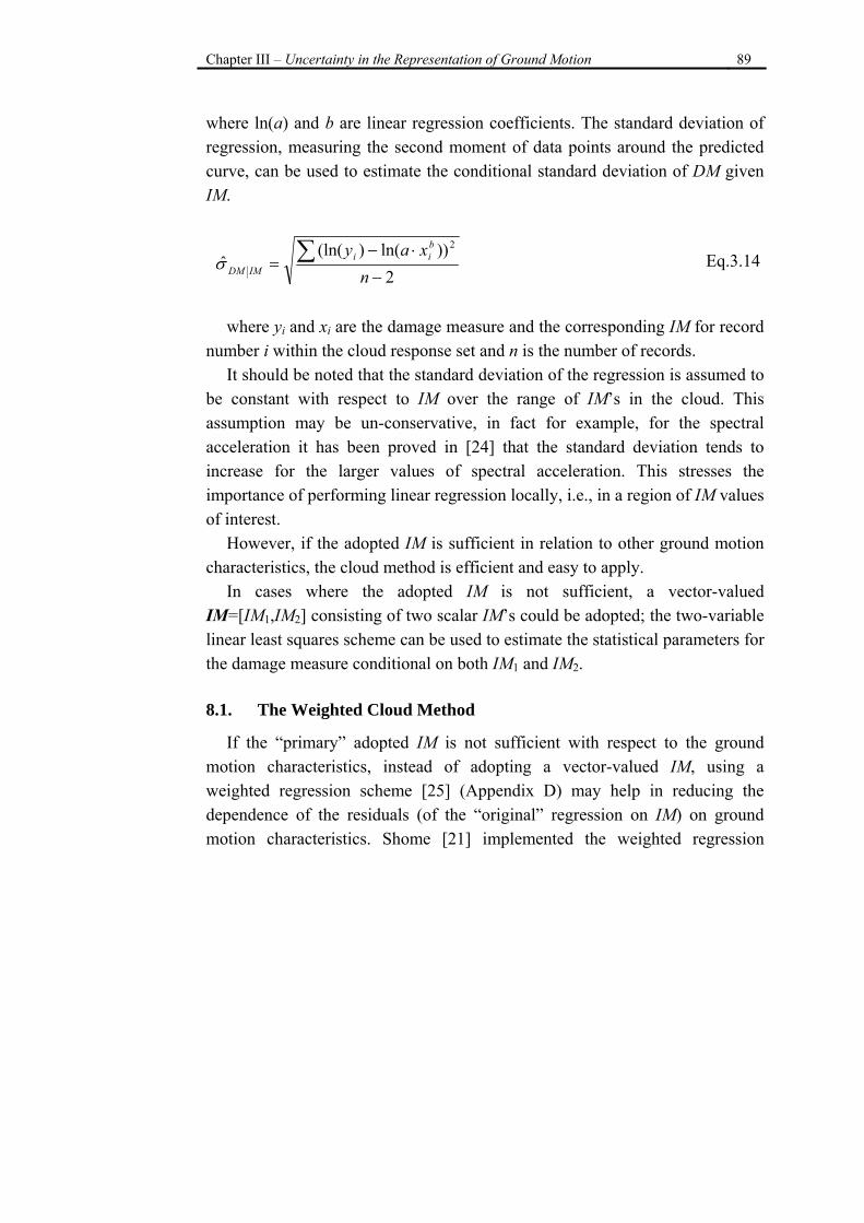
Chapter III – Uncertainty in the Representation of Ground Motion 89
where ln(a) and b are linear regression coefficients. The standard deviation of regression, measuring the second moment of data points around the predicted curve, can be used to estimate the conditional standard deviation of DM given IM.
2))ln()(ln(
ˆ2
−
⋅−= ∑
nxay b
iiIMDMσ Eq.3.14
where yi and xi are the damage measure and the corresponding IM for record
number i within the cloud response set and n is the number of records. It should be noted that the standard deviation of the regression is assumed to
be constant with respect to IM over the range of IM’s in the cloud. This assumption may be un-conservative, in fact for example, for the spectral acceleration it has been proved in [24] that the standard deviation tends to increase for the larger values of spectral acceleration. This stresses the importance of performing linear regression locally, i.e., in a region of IM values of interest.
However, if the adopted IM is sufficient in relation to other ground motion characteristics, the cloud method is efficient and easy to apply.
In cases where the adopted IM is not sufficient, a vector-valued IM=[IM1,IM2] consisting of two scalar IM’s could be adopted; the two-variable linear least squares scheme can be used to estimate the statistical parameters for the damage measure conditional on both IM1 and IM2. 8.1. The Weighted Cloud Method
If the “primary” adopted IM is not sufficient with respect to the ground motion characteristics, instead of adopting a vector-valued IM, using a weighted regression scheme [25] (Appendix D) may help in reducing the dependence of the residuals (of the “original” regression on IM) on ground motion characteristics. Shome [21] implemented the weighted regression
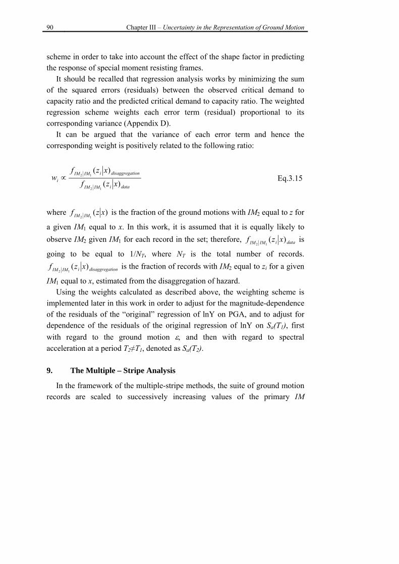
90 Chapter III – Uncertainty in the Representation of Ground Motion
scheme in order to take into account the effect of the shape factor in predicting the response of special moment resisting frames.
It should be recalled that regression analysis works by minimizing the sum of the squared errors (residuals) between the observed critical demand to capacity ratio and the predicted critical demand to capacity ratio. The weighted regression scheme weights each error term (residual) proportional to its corresponding variance (Appendix D).
It can be argued that the variance of each error term and hence the corresponding weight is positively related to the following ratio:
dataiIMIM
tiondisaggregaiIMIMi xzf
xzfw
)(
)(
12
12∝ Eq.3.15
where )(
12xzf IMIM is the fraction of the ground motions with IM2 equal to z for
a given IM1 equal to x. In this work, it is assumed that it is equally likely to observe IM2 given IM1 for each record in the set; therefore, dataiIMIM xzf )(
12 is
going to be equal to 1/NT, where NT is the total number of records.
tiondisaggregaiIMIM xzf )(12
is the fraction of records with IM2 equal to zi for a given
IM1 equal to x, estimated from the disaggregation of hazard. Using the weights calculated as described above, the weighting scheme is
implemented later in this work in order to adjust for the magnitude-dependence of the residuals of the “original” regression of lnY on PGA, and to adjust for dependence of the residuals of the original regression of lnY on Sa(T1), first with regard to the ground motion ε, and then with regard to spectral acceleration at a period T2≠T1, denoted as Sa(T2). 9. The Multiple – Stripe Analysis
In the framework of the multiple-stripe methods, the suite of ground motion records are scaled to successively increasing values of the primary IM
Chapter III – Uncertainty in the Representation of Ground Motion 91
parameter. The set of corresponding structural damage measures calculated for each primary IM value can be referred to as the stripe response for the IM level. The statistical properties of the stripe responses for various IM levels, can be evaluated based on the response to the suite of records, in order to estimate the fragility using equation 3.3.
In cases where the adopted IM is not sufficient, a vector-valued IM=[IM1,IM2] consisting of two scalar IM’s could be adopted. In this case the linear regression analysis can be employed in order to investigate the dependence of the stripe response for each IM1 level on the secondary IM2 parameter. In contrast to the cloud method, the constant coefficients a and b and the standard deviation of the regression residuals, estimated from the observed prediction errors, are re-estimated at every IM1 stripe and depend on the IM1 value at each stripe. 9.1. The Weighted Multiple-Stripe Analysis
Also in the framework of the multiple-stripe analysis, if the “primary” adopted IM is not sufficient with respect to the ground motion characteristics, instead of adopting a vector-valued IM, a procedure similar to the one used in the weighted cloud method can be employed, in order to account for additional information available on the correlation between the adopted primary IM and a candidate secondary IM (e.g, the information extracted from seismic disaggregation). In fact, for a given suite of ground motion records, one could re-weight the stripe response in relation to the conditional probability distribution f(IM2|IM1) at each IM1 level. This approximate method, which has been proposed by Shome and Cornell [21] and Jalayer [24], incorporates the available information about a secondary IM given that the IM1 is known, in the framework of seismic assessments based on the scalar intensity measure IM1.
The first and second central moment (i.e., expected value and variance) of the stripe response for each IM level can be calculated as described in the following. It can be recalled first that the sample average and the sample variance of the relevant damage measure Y can be calculated as:
92 Chapter III – Uncertainty in the Representation of Ground Motion
∑==TN
iiY
NYEY
T
1][ Eq.3.16
222 )(-][ YYEsY = Eq.3.17
where ][⋅E denotes the expected value (mean) estimated by the sample average. The above equations can also be applied to the natural logarithm of the relevant damage measure for a given IM level, x:
∑=≅TN
iiIMY Y
NIMYEx
T
1][ln)(ˆlnη Eq.3.18
222ln
2 ])IM[ln(-]IM[lnˆ YEYEYY == σβ Eq.3.19
where the (log of) median has been approximated by the sample average of the logarithm of the response. Nevertheless, for a lognormal variable, the mean of the logarithm is exactly equal to the logarithm of the median.
Expanding the estimated median and the standard deviation (of the logarithm) with respect to IM2, the mean of the logarithm of the stripe response can also be calculated as:
∑=
=
=≅η
2
21
1
1|21
|
)|(.],|),([ln
)]([ln)(ˆlnIMN
jjIMIMj
IMY
xzfIMIMzxYE
xYEx
Eq.3.20
where )(ˆ ⋅η denotes the estimated median for the stripe response. For a selection consisting of NT ground motion records the above expression can be expanded by dividing the chosen records into
2IMN bins, in which each bin is represented
by value, zj. The E[ln Y(x, zj)] is the estimated conditional mean (i.e., sample average) for the natural logarithm of response in each bin, represented by value,
Chapter III – Uncertainty in the Representation of Ground Motion 93
zj, for a given IM1 value, x and )|(12 | xzf jIMIM is the probability that IM2 is
equal to z (in bin j) given IM1 equal to x (e.g. it can be obtained from disaggregation).
In a similar manner, the conditional variance of the natural logarithm of response for a given IM1=x, can be expanded with respect to a candidate secondary intensity measure, IM2, as:
21
|2122
|ln
])|[ln(
)|(],|)),([(ln)(ˆ 2
211
IMYE
xzfIMIMzxYExIMN
jjIMIMjIMY
−
−⋅≅β ∑=
Eq.3.21
Here, E[(lnY(x, zj))2|IM1,IM2] denotes the expected value estimated by the
conditional sample average of the squares of the natural logarithm (i.e., the estimated second moment) of structural response to ground motions in each bin represented by the value zj (for a given IM1 = x).
As it was stated in the beginning of this work, an intensity measure IM1 is sufficient if it renders the critical demand to capacity ratio or the damage measure considered conditionally independent of the ground motion characteristics, for a given intensity level (e.g., IM1=x). The statistical equivalent to this statement is to establish that the conditional probability distribution for the critical demand to capacity ratio of the structure for a given intensity level is independent of other ground motion characteristics, namely:
),( )(211 ,|| jIMIMYIMY zxfxf = Eq.3.22
for any zj value.
The sufficiency criterion can be also “approximated” in terms of the (conditional) statistical moments of the response (e.g., conditional mean and variance) being independent of the ground motion characteristics. For example, a “first-order measure” of the sufficiency criterion can be obtained by
94 Chapter III – Uncertainty in the Representation of Ground Motion
establishing that the first (conditional) moment of the response for a given IM1 level, x, is independent of other ground motion characteristics:
],|),([ln]|)([ln 211 IMIMzxYEIMxYE j= Eq.3.23
for all zj value.
For a lognormal random variable, the above equation can be written as the equality of the medians:
]),([ln)(ˆln1 jIMY zxYEx =η Eq.3.24
If an IM is sufficient, it can be demonstrated that the two sides of equation
3.20 will be always equal (by substituting ),(ˆ21 ,| jIMIMY zxη by )(ˆ
1| xIMYη in the
equation) and does not depend on the probability distribution 12 |IMIMf :
∑
∑
=
=
⋅=
=⋅=
2
121
2
1211
1||
1|||
)|( )(ˆn
)|( )(ˆn )(ˆn
IM
IM
N
jjIMIMIMY
N
jjIMIMIMYIMY
xzfxl
xzfxlxl
η
ηη
Eq.3.25
The above conclusion is based on the fact that the sum of the fractions
)|(12 | xzf jIMIM is equal to unity. A “second order measure” of sufficiency
criterion can be expressed in terms of the (conditional) second moment of the response:
],|)),([(ln]|))([(ln 212
12 IMIMzxYEIMxYE j= Eq.3.26
for all zj value.
Chapter III – Uncertainty in the Representation of Ground Motion 95
Similarly, it can be demonstrated that the two sides of equation 3.21 will always be equal, independent of )|(
12 | xzf jIMIM , if the second-order
approximation to sufficiency are established. 9.2. Accounting for Collapse Cases in Multiple-Stripe Analysis
When multiple-stripe analysis is performed for high IM levels, it happens quite often that the structural analysis cases do not yield meaningful values. This could either imply that the structure has lost its load bearing capacity or may simply signal a numerical in-convergence. Since both cases are characterized by very large damage measure values, they are both referred to, for simplicity, as the “collapse cases”.
In this study the logistic regression is used in order take into account the collapse cases, that happen in the structural analysis for increasing level of IM1. In order to explicitly take into account collapse cases the stripe response is divided into two parts, namely, the non-collapse and the collapse parts. As far as it regards the non-collapse part of the stripe response, one could proceed as described in the previous section. For example, the linear least squares can be applied to the non-collapse part in order to model the correlation between IM1
and IM2. Alternatively, it can be divided into different bins. The logistic regression [25] is applied to the collapse data in order to predict the probability collapse as a function of the second intensity measure IM2, rather than estimating the probability of collapse simply as the fraction of records in an IM1 stripe that cause collapse (in the latter case, probability of collapse will not depend on IM2).
Using the indicator variable C to designate occurrence of collapse (C equals 1 if the record causes collapse and 0 otherwise), the following functional form is fitted:
zxbxa
zxbxa
eezIMxIMCP ⋅+
⋅+
+=== )()(
)()(
21 1),( Eq.3.27
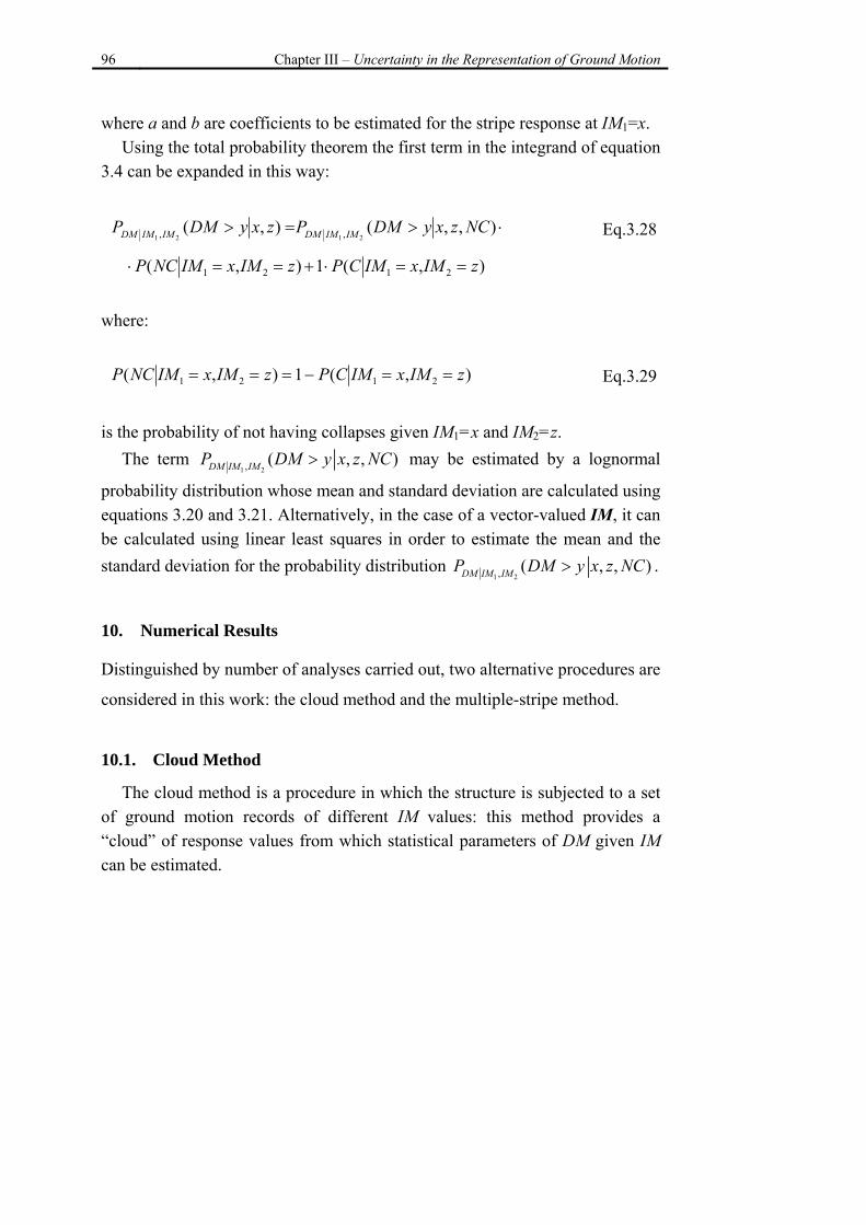
96 Chapter III – Uncertainty in the Representation of Ground Motion
where a and b are coefficients to be estimated for the stripe response at IM1=x. Using the total probability theorem the first term in the integrand of equation
3.4 can be expanded in this way:
⋅>=> ),,(),(2121 ,, NCzxyDMPzxyDMP IMIMDMIMIMDM Eq.3.28
),(1),( 2121 zIMxIMCPzIMxIMNCP ==⋅+==⋅ where:
),(1),( 2121 zIMxIMCPzIMxIMNCP ==−=== Eq.3.29
is the probability of not having collapses given IM1=x and IM2=z.
The term 1 2, ( , , )DM IM IMP DM y x z NC> may be estimated by a lognormal
probability distribution whose mean and standard deviation are calculated using equations 3.20 and 3.21. Alternatively, in the case of a vector-valued IM, it can be calculated using linear least squares in order to estimate the mean and the standard deviation for the probability distribution
1 2, ( , , )DM IM IMP DM y x z NC> .
10. Numerical Results
Distinguished by number of analyses carried out, two alternative procedures are
considered in this work: the cloud method and the multiple-stripe method.
10.1. Cloud Method
The cloud method is a procedure in which the structure is subjected to a set of ground motion records of different IM values: this method provides a “cloud” of response values from which statistical parameters of DM given IM can be estimated.
Chapter III – Uncertainty in the Representation of Ground Motion 97
10.1.1. Record Selection A (Sel_A)
For record selection A (Sel_A) the primary IM used in this study in a scalar form is the peak ground acceleration (PGA), that can be regarded as a scale factor of the single spectrum of the selection of records, paired in vector form, with magnitude (M), since it can be regarded as a “shape factor” of the single spectrum.
In Figure 3.4a the results obtained using the cloud method for the PGA and Y data pairs are shown. As stated in advance, in order to establish sufficiency of the primary IM and the effectiveness of ground motion characteristic variables as additional regression variables, a graphical statistical tool known as the residual-residual plot is used. The main advantage of the residual-residual plots is that they offer visual means for judging the improvement caused by an additional regression variable. In Figure 3.4b the residual-residual plot related to the introduction of magnitude as additional intensity measure, and the p-values calculated for the hypotheses test are shown. Judging from both the p-value and the reported b value, a significant positive trend in the plot can be observed: this indicates that, as expected, the peak ground acceleration is not sufficient with respect to the magnitude. Figure 3.4c shows the results obtained by the cloud method adopting the vector intensity measure [PGA, M]. The multiple regression is used to predict the structural damage measure as a function of both peak ground acceleration and magnitude.
98 Chapter III – Uncertainty in the Representation of Ground Motion
Figure 3.4. (a) Simple regression PGA-Y, Sel_A. (b) Residual-residual plot for magnitude
as a second independent variable. (c) Multiple regression PGA-M-Y , Sel_A. (d) Weighted regression PGA-M-Y, Sel_A.
It would be interesting to study how the seismic risk, represented herein by
the mean annual frequency of exceeding the structural damage measure, is affected by the weighed regression scheme. The results of weighted regression (Figure 3.4d) can be used in order to predict the conditional mean and standard deviation of the damage measure as a function of PGA; these parameters are then incorporated in equation 3.3 in order to calculate the structural fragility. The mean annual frequency of exceeding the structural damage measure can be calculated from equation 3.2 by integrating the structural fragility and the peak ground acceleration hazard curve (Figure 3.11b) (extracted from the site of
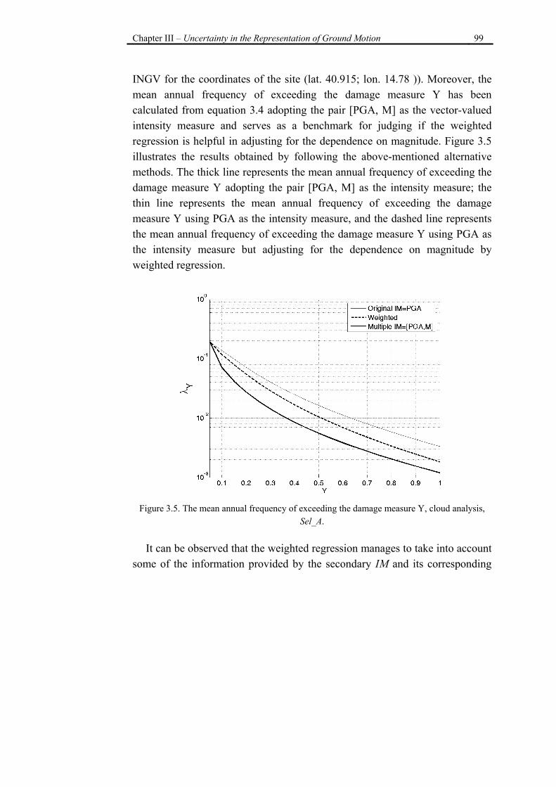
Chapter III – Uncertainty in the Representation of Ground Motion 99
INGV for the coordinates of the site (lat. 40.915; lon. 14.78 )). Moreover, the mean annual frequency of exceeding the damage measure Y has been calculated from equation 3.4 adopting the pair [PGA, M] as the vector-valued intensity measure and serves as a benchmark for judging if the weighted regression is helpful in adjusting for the dependence on magnitude. Figure 3.5 illustrates the results obtained by following the above-mentioned alternative methods. The thick line represents the mean annual frequency of exceeding the damage measure Y adopting the pair [PGA, M] as the intensity measure; the thin line represents the mean annual frequency of exceeding the damage measure Y using PGA as the intensity measure, and the dashed line represents the mean annual frequency of exceeding the damage measure Y using PGA as the intensity measure but adjusting for the dependence on magnitude by weighted regression.
Figure 3.5. The mean annual frequency of exceeding the damage measure Y, cloud analysis,
Sel_A.
It can be observed that the weighted regression manages to take into account some of the information provided by the secondary IM and its corresponding
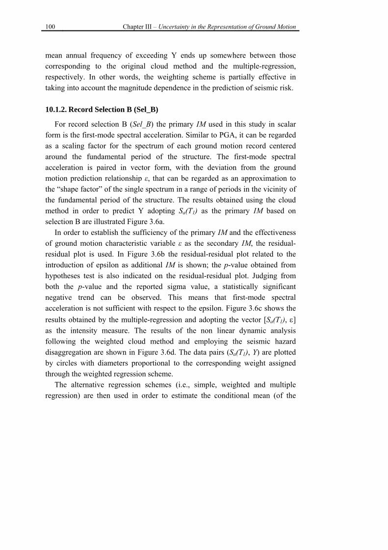
100 Chapter III – Uncertainty in the Representation of Ground Motion
mean annual frequency of exceeding Y ends up somewhere between those corresponding to the original cloud method and the multiple-regression, respectively. In other words, the weighting scheme is partially effective in taking into account the magnitude dependence in the prediction of seismic risk. 10.1.2. Record Selection B (Sel_B)
For record selection B (Sel_B) the primary IM used in this study in scalar form is the first-mode spectral acceleration. Similar to PGA, it can be regarded as a scaling factor for the spectrum of each ground motion record centered around the fundamental period of the structure. The first-mode spectral acceleration is paired in vector form, with the deviation from the ground motion prediction relationship ε, that can be regarded as an approximation to the “shape factor” of the single spectrum in a range of periods in the vicinity of the fundamental period of the structure. The results obtained using the cloud method in order to predict Y adopting Sa(T1) as the primary IM based on selection B are illustrated Figure 3.6a.
In order to establish the sufficiency of the primary IM and the effectiveness of ground motion characteristic variable ε as the secondary IM, the residual-residual plot is used. In Figure 3.6b the residual-residual plot related to the introduction of epsilon as additional IM is shown; the p-value obtained from hypotheses test is also indicated on the residual-residual plot. Judging from both the p-value and the reported sigma value, a statistically significant negative trend can be observed. This means that first-mode spectral acceleration is not sufficient with respect to the epsilon. Figure 3.6c shows the results obtained by the multiple-regression and adopting the vector [Sa(T1), ε] as the intensity measure. The results of the non linear dynamic analysis following the weighted cloud method and employing the seismic hazard disaggregation are shown in Figure 3.6d. The data pairs (Sa(T1), Y) are plotted by circles with diameters proportional to the corresponding weight assigned through the weighted regression scheme.
The alternative regression schemes (i.e., simple, weighted and multiple regression) are then used in order to estimate the conditional mean (of the
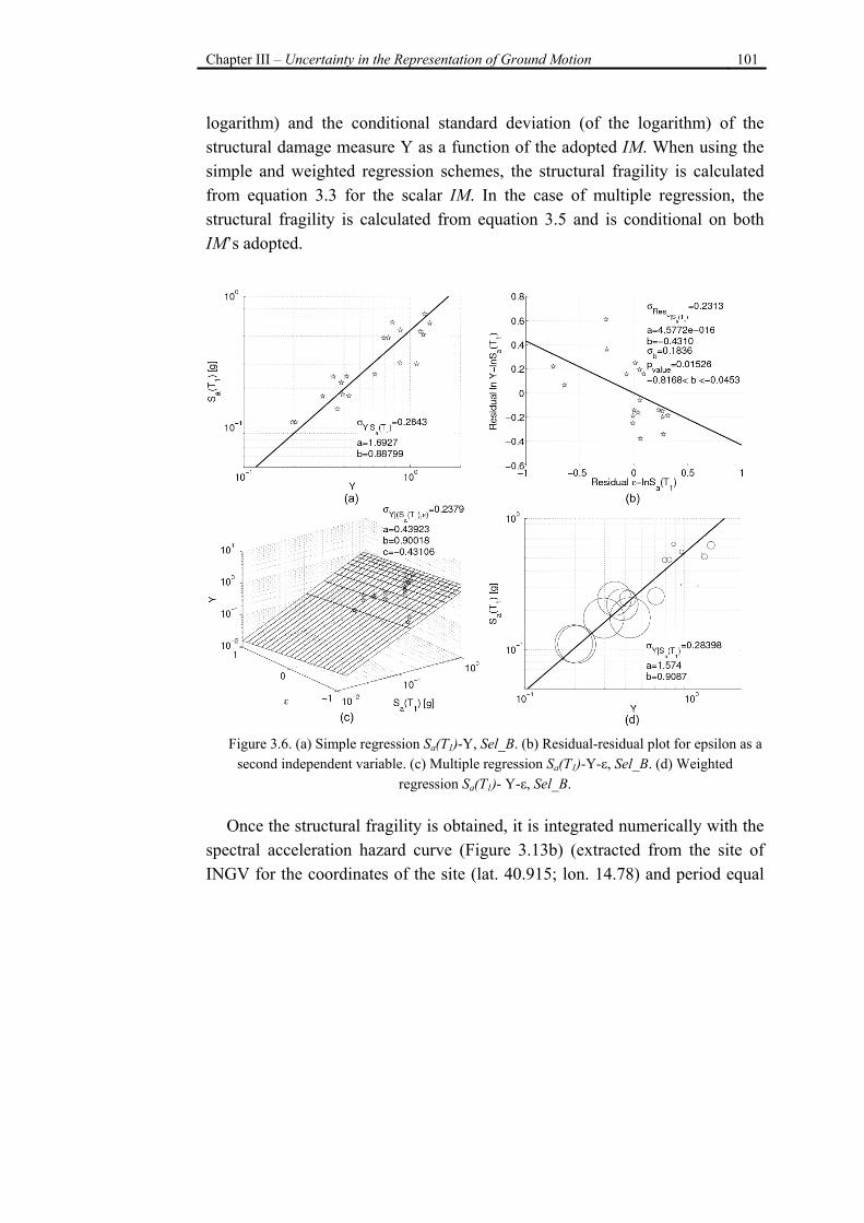
Chapter III – Uncertainty in the Representation of Ground Motion 101
logarithm) and the conditional standard deviation (of the logarithm) of the structural damage measure Y as a function of the adopted IM. When using the simple and weighted regression schemes, the structural fragility is calculated from equation 3.3 for the scalar IM. In the case of multiple regression, the structural fragility is calculated from equation 3.5 and is conditional on both IM’s adopted.
Figure 3.6. (a) Simple regression Sa(T1)-Y, Sel_B. (b) Residual-residual plot for epsilon as a
second independent variable. (c) Multiple regression Sa(T1)-Y-ε, Sel_B. (d) Weighted regression Sa(T1)- Y-ε, Sel_B.
Once the structural fragility is obtained, it is integrated numerically with the
spectral acceleration hazard curve (Figure 3.13b) (extracted from the site of INGV for the coordinates of the site (lat. 40.915; lon. 14.78) and period equal
102 Chapter III – Uncertainty in the Representation of Ground Motion
to 0.75 seconds) in order to calculate the mean annual frequency of exceeding the damage measure Y or the seismic risk curve. Figure 3.7 illustrates the seismic risk curve calculated using the above-mentioned alternative methods. It can be observed that the seismic risk curve calculated using the weighted regression manages to adjust partially for the dependence on epsilon. Obviously, the resulting improvement depends both on the spread of the epsilon values for the selected ground motion records and the ground motion prediction relationship used in the hazard/disaggregation analysis (Figure 3.3b).
Figure 3.7. The mean annual frequency of exceeding the damage measure Y, cloud analysis,
Sel_B.
The choice of epsilon as the secondary IM has been inspired by the fact that it acts as a proxy for spectral shape in the vicinity of the fundamental period of the structure. Therefore, it is interesting to investigate also the dependence of the damage measure Y given Sa(T1) on spectral acceleration at another period T2 ≠ T1, (Sa(T2)), in order to consider in an explicit way the shape of the elastic acceleration spectrum. The procedure followed for establishing the dependence of Y given Sa(T1)), on Sa(T2) is similar to the one followed in order to
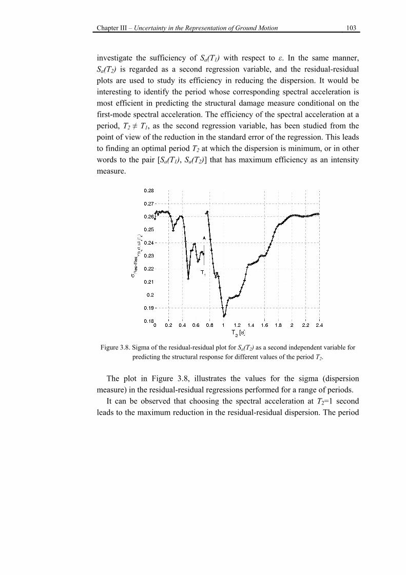
Chapter III – Uncertainty in the Representation of Ground Motion 103
investigate the sufficiency of Sa(T1) with respect to ε. In the same manner, Sa(T2) is regarded as a second regression variable, and the residual-residual plots are used to study its efficiency in reducing the dispersion. It would be interesting to identify the period whose corresponding spectral acceleration is most efficient in predicting the structural damage measure conditional on the first-mode spectral acceleration. The efficiency of the spectral acceleration at a period, T2 ≠ T1, as the second regression variable, has been studied from the point of view of the reduction in the standard error of the regression. This leads to finding an optimal period T2 at which the dispersion is minimum, or in other words to the pair [Sa(T1), Sa(T2)] that has maximum efficiency as an intensity measure.
Figure 3.8. Sigma of the residual-residual plot for Sa(T2) as a second independent variable for
predicting the structural response for different values of the period T2.
The plot in Figure 3.8, illustrates the values for the sigma (dispersion measure) in the residual-residual regressions performed for a range of periods.
It can be observed that choosing the spectral acceleration at T2=1 second leads to the maximum reduction in the residual-residual dispersion. The period
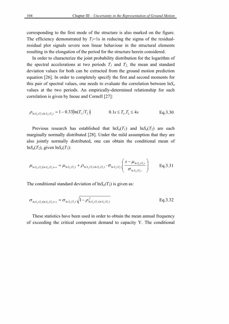
104 Chapter III – Uncertainty in the Representation of Ground Motion
corresponding to the first mode of the structure is also marked on the figure. The efficiency demonstrated by T2=1s in reducing the sigma of the residual-residual plot signals severe non linear behaviour in the structural elements resulting in the elongation of the period for the structure herein considered.
In order to characterize the joint probability distribution for the logarithm of the spectral accelerations at two periods T1 and T2, the mean and standard deviation values for both can be extracted from the ground motion prediction equation [26]. In order to completely specify the first and second moments for this pair of spectral values, one needs to evaluate the correlation between lnSa values at the two periods. An empirically-determined relationship for such correlation is given by Inoue and Cornell [27]:
)ln(33.01 21)(ln),(ln 21TTTSTS aa
−=ρ sTTs 4,1.0 21 ≤≤ Eq.3.30
Previous research has established that lnSa(T1) and lnSa(T2) are each
marginally normally distributed [28]. Under the mild assumption that they are also jointly normally distributed, one can obtain the conditional mean of lnSa(T2), given lnSa(T1):
⎟⎟⎠
⎞⎜⎜⎝
⎛ −⋅+==
)(ln
)(ln)(ln)(ln),(ln)(ln)(ln)(ln
1
1
221221TS
TSTSTSTSTSxTSTS
a
a
aaaaaa
xσ
µσρµµ Eq.3.31
The conditional standard deviation of lnSa(T2) is given as:
2)(ln),(ln)(ln)(ln)(ln 21221
1 TSTSTSxTSTS aaaaaρσσ −== Eq.3.32
These statistics have been used in order to obtain the mean annual frequency
of exceeding the critical component demand to capacity Y. The conditional
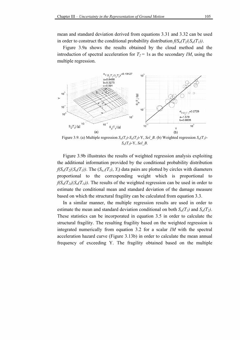
Chapter III – Uncertainty in the Representation of Ground Motion 105
mean and standard deviation derived from equations 3.31 and 3.32 can be used in order to construct the conditional probability distribution f(Sa(T2)|Sa(T1)).
Figure 3.9a shows the results obtained by the cloud method and the introduction of spectral acceleration for T2 = 1s as the secondary IM, using the multiple regression.
Figure 3.9. (a) Multiple regression Sa(T1)-Sa(T2)-Y, Sel_B. (b) Weighted regression Sa(T1)-
Sa(T2)-Y, Sel_B.
Figure 3.9b illustrates the results of weighted regression analysis exploiting the additional information provided by the conditional probability distribution f(Sa(T2)|Sa(T1)). The (Sa,i(T1), Yi) data pairs are plotted by circles with diameters proportional to the corresponding weight which is proportional to f(Sa(T2i)|Sa(T1i)). The results of the weighted regression can be used in order to estimate the conditional mean and standard deviation of the damage measure based on which the structural fragility can be calculated from equation 3.3.
In a similar manner, the multiple regression results are used in order to estimate the mean and standard deviation conditional on both Sa(T1) and Sa(T2). These statistics can be incorporated in equation 3.5 in order to calculate the structural fragility. The resulting fragility based on the weighted regression is integrated numerically from equation 3.2 for a scalar IM with the spectral acceleration hazard curve (Figure 3.13b) in order to calculate the mean annual frequency of exceeding Y. The fragility obtained based on the multiple
106 Chapter III – Uncertainty in the Representation of Ground Motion
regression is integrated with the spectral acceleration hazard in equation 3.4 for a vector IM in order to provide the seismic risk curve. Figure 3.10 illustrates the seismic risk curves calculated by following the alternative approaches just discussed.
Figure 3.10. The mean annual frequency of exceeding the damage measure Y, cloud analysis,
Sel_B.
It can be observed that there is only a small gain in information resulting from incorporating the correlation between the two spectral values inside the weighted regression scheme. The same as the case of IM2=ε, the weights applied inside the weighted regression are quite sensitive to both interval covered by the Sa(T2) values of the selection of records and the characterization of f(Sa(T2)|Sa(T1)). 10.2. Multiple-Stripe Analysis
The results of multiple-stripe analysis are used in order to investigate the efficiency of the weighting scheme based on the information provided by
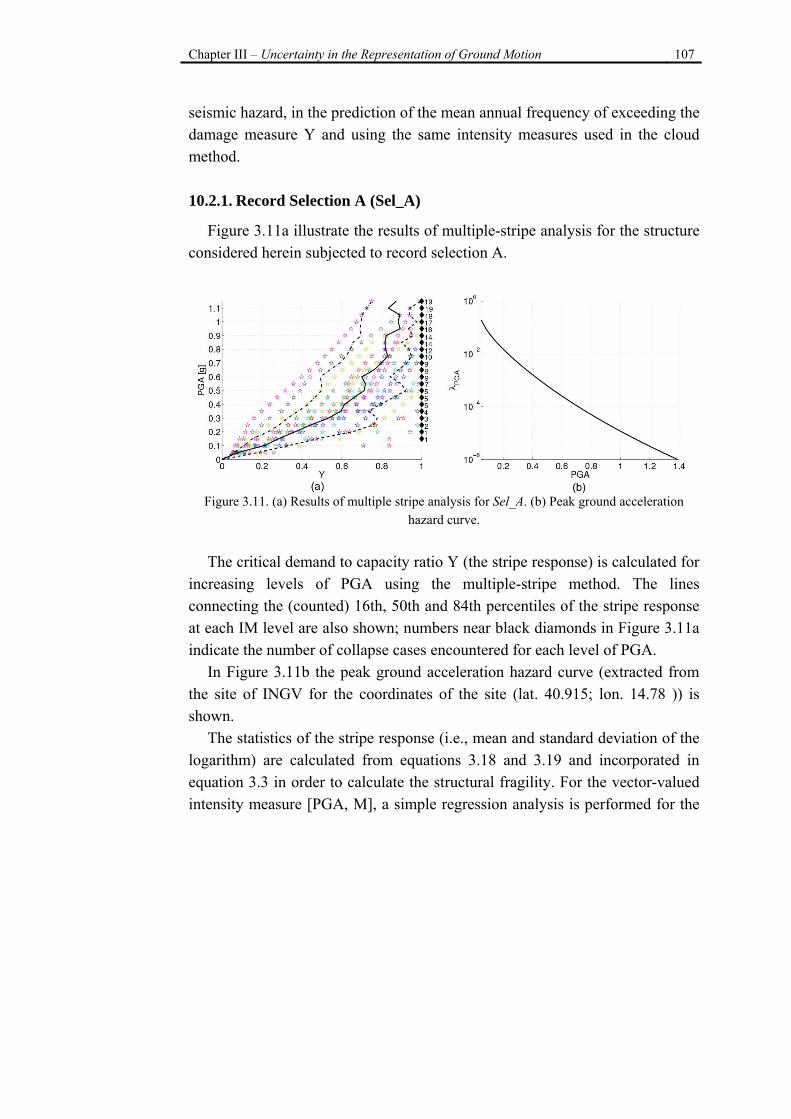
Chapter III – Uncertainty in the Representation of Ground Motion 107
seismic hazard, in the prediction of the mean annual frequency of exceeding the damage measure Y and using the same intensity measures used in the cloud method. 10.2.1. Record Selection A (Sel_A)
Figure 3.11a illustrate the results of multiple-stripe analysis for the structure considered herein subjected to record selection A.
Figure 3.11. (a) Results of multiple stripe analysis for Sel_A. (b) Peak ground acceleration hazard curve.
The critical demand to capacity ratio Y (the stripe response) is calculated for
increasing levels of PGA using the multiple-stripe method. The lines connecting the (counted) 16th, 50th and 84th percentiles of the stripe response at each IM level are also shown; numbers near black diamonds in Figure 3.11a indicate the number of collapse cases encountered for each level of PGA.
In Figure 3.11b the peak ground acceleration hazard curve (extracted from the site of INGV for the coordinates of the site (lat. 40.915; lon. 14.78 )) is shown.
The statistics of the stripe response (i.e., mean and standard deviation of the logarithm) are calculated from equations 3.18 and 3.19 and incorporated in equation 3.3 in order to calculate the structural fragility. For the vector-valued intensity measure [PGA, M], a simple regression analysis is performed for the
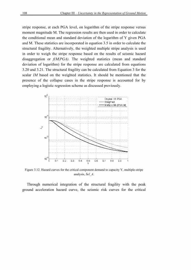
108 Chapter III – Uncertainty in the Representation of Ground Motion
stripe response, at each PGA level, on logarithm of the stripe response versus moment magnitude M. The regression results are then used in order to calculate the conditional mean and standard deviation of the logarithm of Y given PGA and M. These statistics are incorporated in equation 3.5 in order to calculate the structural fragility. Alternatively, the weighted multiple stripe analysis is used in order to weigh the stripe response based on the results of seismic hazard disaggregation or f(M|PGA). The weighted statistics (mean and standard deviation of logarithm) for the stripe response are calculated from equations 3.20 and 3.21. The structural fragility can be calculated from Equation 3 for the scalar IM based on the weighted statistics. It should be mentioned that the presence of the collapse cases in the stripe response is accounted for by employing a logistic regression scheme as discussed previously.
Figure 3.12. Hazard curves for the critical component demand to capacity Y, multiple-stripe
analysis, Sel_A.
Through numerical integration of the structural fragility with the peak ground acceleration hazard curve, the seismic risk curves for the critical
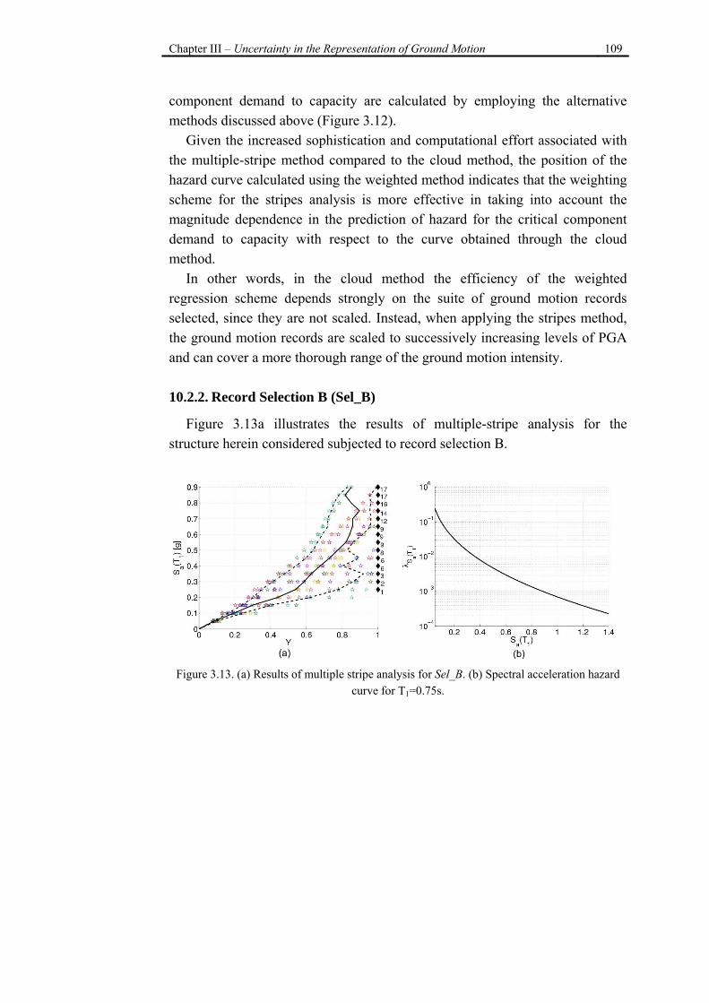
Chapter III – Uncertainty in the Representation of Ground Motion 109
component demand to capacity are calculated by employing the alternative methods discussed above (Figure 3.12).
Given the increased sophistication and computational effort associated with the multiple-stripe method compared to the cloud method, the position of the hazard curve calculated using the weighted method indicates that the weighting scheme for the stripes analysis is more effective in taking into account the magnitude dependence in the prediction of hazard for the critical component demand to capacity with respect to the curve obtained through the cloud method.
In other words, in the cloud method the efficiency of the weighted regression scheme depends strongly on the suite of ground motion records selected, since they are not scaled. Instead, when applying the stripes method, the ground motion records are scaled to successively increasing levels of PGA and can cover a more thorough range of the ground motion intensity. 10.2.2. Record Selection B (Sel_B)
Figure 3.13a illustrates the results of multiple-stripe analysis for the structure herein considered subjected to record selection B.
Figure 3.13. (a) Results of multiple stripe analysis for Sel_B. (b) Spectral acceleration hazard
curve for T1=0.75s.
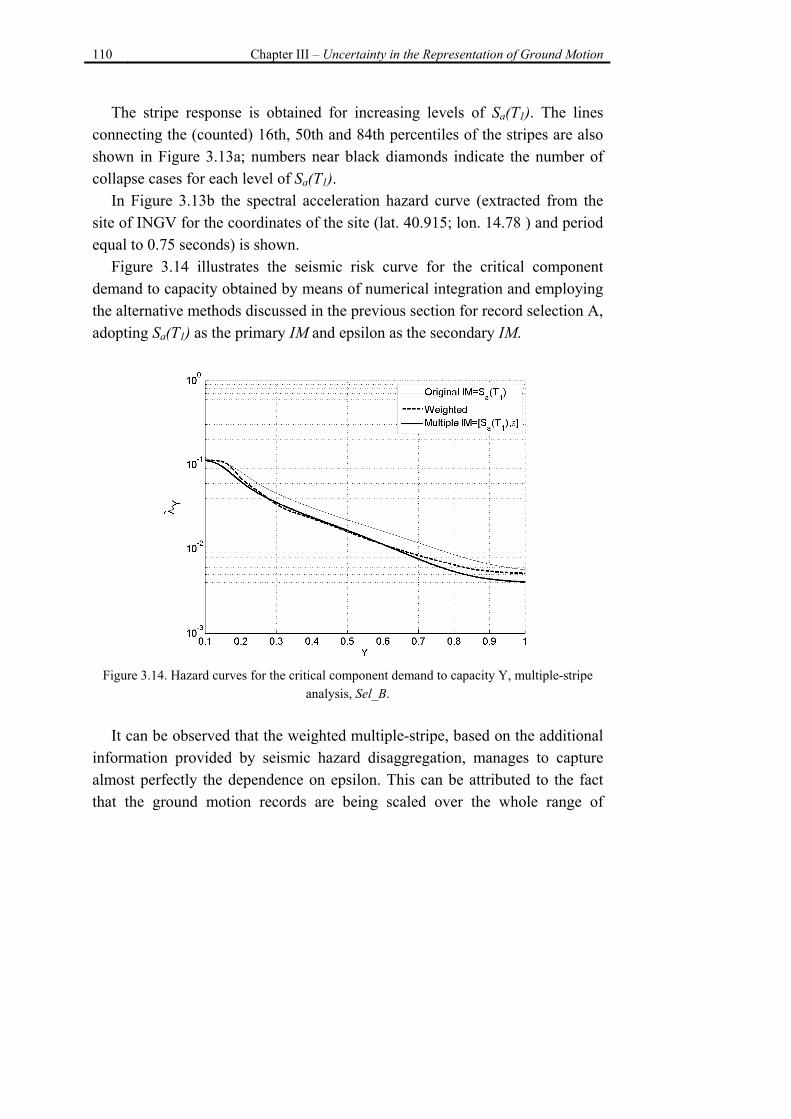
110 Chapter III – Uncertainty in the Representation of Ground Motion
The stripe response is obtained for increasing levels of Sa(T1). The lines connecting the (counted) 16th, 50th and 84th percentiles of the stripes are also shown in Figure 3.13a; numbers near black diamonds indicate the number of collapse cases for each level of Sa(T1).
In Figure 3.13b the spectral acceleration hazard curve (extracted from the site of INGV for the coordinates of the site (lat. 40.915; lon. 14.78 ) and period equal to 0.75 seconds) is shown.
Figure 3.14 illustrates the seismic risk curve for the critical component demand to capacity obtained by means of numerical integration and employing the alternative methods discussed in the previous section for record selection A, adopting Sa(T1) as the primary IM and epsilon as the secondary IM.
Figure 3.14. Hazard curves for the critical component demand to capacity Y, multiple-stripe
analysis, Sel_B.
It can be observed that the weighted multiple-stripe, based on the additional information provided by seismic hazard disaggregation, manages to capture almost perfectly the dependence on epsilon. This can be attributed to the fact that the ground motion records are being scaled over the whole range of
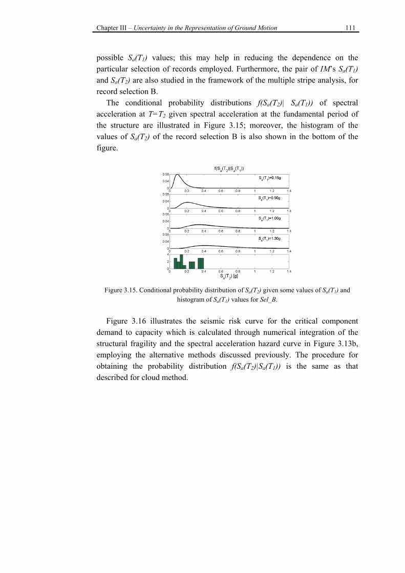
Chapter III – Uncertainty in the Representation of Ground Motion 111
possible Sa(T1) values; this may help in reducing the dependence on the particular selection of records employed. Furthermore, the pair of IM’s Sa(T1) and Sa(T2) are also studied in the framework of the multiple stripe analysis, for record selection B.
The conditional probability distributions f(Sa(T2)| Sa(T1)) of spectral acceleration at T=T2 given spectral acceleration at the fundamental period of the structure are illustrated in Figure 3.15; moreover, the histogram of the values of Sa(T2) of the record selection B is also shown in the bottom of the figure.
Figure 3.15. Conditional probability distribution of Sa(T2) given some values of Sa(T1) and
histogram of Sa(T1) values for Sel_B.
Figure 3.16 illustrates the seismic risk curve for the critical component demand to capacity which is calculated through numerical integration of the structural fragility and the spectral acceleration hazard curve in Figure 3.13b, employing the alternative methods discussed previously. The procedure for obtaining the probability distribution f(Sa(T2)|Sa(T1)) is the same as that described for cloud method.
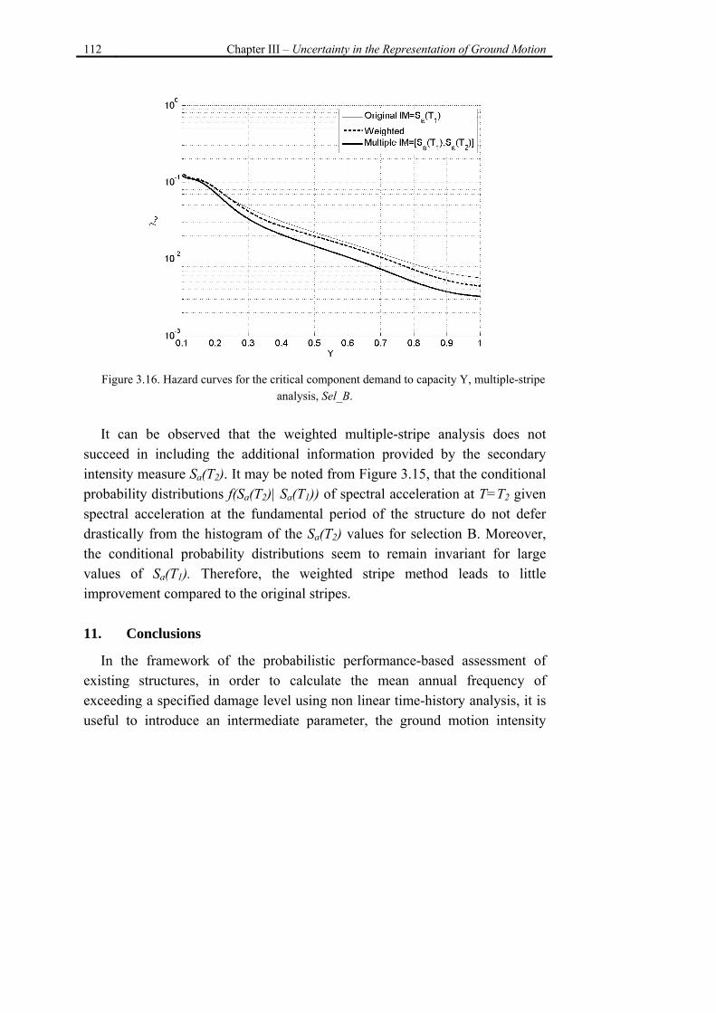
112 Chapter III – Uncertainty in the Representation of Ground Motion
Figure 3.16. Hazard curves for the critical component demand to capacity Y, multiple-stripe
analysis, Sel_B.
It can be observed that the weighted multiple-stripe analysis does not succeed in including the additional information provided by the secondary intensity measure Sa(T2). It may be noted from Figure 3.15, that the conditional probability distributions f(Sa(T2)| Sa(T1)) of spectral acceleration at T=T2 given spectral acceleration at the fundamental period of the structure do not defer drastically from the histogram of the Sa(T2) values for selection B. Moreover, the conditional probability distributions seem to remain invariant for large values of Sa(T1). Therefore, the weighted stripe method leads to little improvement compared to the original stripes. 11. Conclusions
In the framework of the probabilistic performance-based assessment of existing structures, in order to calculate the mean annual frequency of exceeding a specified damage level using non linear time-history analysis, it is useful to introduce an intermediate parameter, the ground motion intensity
Chapter III – Uncertainty in the Representation of Ground Motion 113
measure IM, to relate the ground motion record characteristics to the structural performance. The intensity measure approach is appealing because it allows for (roughly speaking) decoupling the seismic hazard analysis and the structural fragility analysis.
The seismic hazard function, for the adopted IM, can be obtained from the results of site-specific probabilistic seismic hazard analysis or directly from the national seismic maps.
In order to estimate the structural fragility, depending on the amount of structural analysis, two alternative non-linear dynamic analysis procedures can be considered: the cloud method and the multiple-stripe method.
However, the approach based on the introduction of the intensity measure, assumes that structural response depends only upon the chosen IM parameter, and not on any other properties of the ground motion. This required condition is termed “sufficiency” and means that the structural response for a given IM is statistically independent of the ground motion characteristics. This hypothesis must be carefully verified since, if the sufficiency condition is not met, then the probability distribution for the damage measure will not only depend upon IM, but also upon the (other) properties of the records selected for analysis. Hence, in case the properties of the selected records do not reflect, in a realistic manner the records that the real structure will be subjected to, a biased estimate of structural response would be obtained. If the adopted IM is sufficient with respect to other ground motion characteristics, depending on the amount of structural analysis, both cloud and multiple-stripe methods can be implemented in order to evaluate structural fragility. In order to estimate the statistical properties of DM given IM by employing the cloud response, the linear least squares scheme can be applied. Instead, in the framework of multiple-stripes method, the statistical properties of each stripe response, can be evaluated based on the DM values calculated in response to the scaled suite of records for various IM levels.
One effective way to increase the sufficiency of an IM, is to introduce additional parameters, so that the resulting vector-valued IM would describe more completely the properties of the ground motion. In particular, a vector
114 Chapter III – Uncertainty in the Representation of Ground Motion
intensity measure IM=[IM1,IM2] consisting of two parameters can be adopted; IM1 represents the primary intensity measure and IM2 represents the secondary intensity measure that strives to capture the ground motion characteristics not already described by IM1. Also in the case of a bi-variate IM, both cloud and multiple-stripe methods can be implemented in order to evaluate the structural fragility. In the context of the cloud method, the two-variable linear least squares scheme can be used to estimate the statistical parameters for DM conditional on both IM1 and IM2. In the framework of multiple-stripe method the linear regression analysis can be employed on each stripe response in order to investigate the dependence on the secondary IM2 parameter for each IM1 level. A simple statistical and graphical tool known as the residual-residual plots is employed in this work in order to reveal possible dependence of the response DM conditional on the adopted primary IM, on a candidate secondary IM.
In the cases where sufficiency for the primary IM is not established, a weighting scheme based on the results of the seismic hazard analysis for the ground motion characteristic variable(s) can be implemented in the estimation of the structural fragility. This is to adjust for the dependence of the structural response, conditional on the adopted primary IM1, on the candidate secondary IM2. In the context of the cloud method the weighted regression scheme is applied to the cloud response, weighting each square residual term in relation to the conditional probability distribution f(IM2|IM1), obtained through seismic hazard disaggregation. In the framework of the multiple-stripe analysis, an analogous weighting procedure was employed, in order to account for the information available on the correlation between IM1 and a candidate IM2, obtained through seismic hazard disaggregation. In this approach, the stripe response is discretized into into a set of IM2 bins; each bin is then weighted by the probability f(IM2| IM1) obtained from seismic hazard analysis..
The conditional probability distributions for magnitude given peak ground acceleration f(M|PGA) and for epsilon of the ground motion prediction relation given the spectral acceleration at first mode, f(ε|Sa(T1)) have been calculated
Chapter III – Uncertainty in the Representation of Ground Motion 115
through the disaggregation of the seismic hazard for the site of the case-study structure using the Bayesian probabilistic framework.
The implication of using the weighting scheme has been studied in terms of seismic risk represented herein by the mean annual frequency of exceeding the critical component demand to capacity ratio (Y), using both cloud and multiple-stripe methods. In order to evaluate the efficiency of the weighting scheme the seismic risk curve obtained was compared with the curves obtained by adopting the scalar primary IM1 and the vector valued IM=[IM1,IM2].
In particular, as scalar primary IM’s, the peak ground acceleration PGA and the spectral acceleration at the first mode Sa(T1) were considered. The weighting scheme was applied to adjust for the magnitude-dependence of the structural response conditional on PGA. Alternatively, considering Sa(T1) as the primary IM, the weighting scheme was used to adjust for the epsilon-dependence of the structural response conditional on Sa(T1) . Finally, the weighting scheme is used to take into account the spectral shape-dependence of the structural response conditional on Sa(T1) at a period T2 ≠ T1, (Sa(T2)). The same pairs of intensity measures were also considered as vector-valued IM. The seismic risk curves calculated by adopting the vector-valued IM’s were used to benchmark the efficiency of the weighting scheme.
Among all the analysed cases, it is observed that the weighting scheme manages to take into account some of the information provided by the secondary IM and its corresponding mean annual frequency of exceeding Y ends up somewhere between those obtained adopting the scalar primary IM and the vector-valued IM consisting of the primary and the secondary intensity measures, respectively. However, the weighting scheme proves much more efficient for multiple-stripe analysis compared to the cloud analysis. This can be attributed to the fact that, the multiple-stripe analysis spans over a wider range of ground motion intensity levels and therefore proves less sensitive to the selection of ground motion records compared to the cloud method. On the other hand, the success of the weighting scheme for the cloud method depends on the selection of records. In general, it can be observed that the weighted scheme enhances the assessment of the mean annual frequency of exceeding a

116 Chapter III – Uncertainty in the Representation of Ground Motion
specified damage level for the structure considered herein and allows a more accurate estimation of the structural response with a limited number of analyses.
Chapter III – Uncertainty in the Representation of Ground Motion 117
12. References
[1] Iervolino I., Maddaloni G., Cosenza E. (2008). “Eurocode 8 compliant real record sets for seismic analysis of structures”, Journal of Earthquake Engineering, 12(1): 54–60.
[2] Iervolino I., Maddaloni G., Cosenza E. (2009). A note on selection of time-histories for seismic analysis of bridges in Eurocode 8. Journal of Earthquake Engineering. (in press)
[3] Bazzurro P., Cornell C.A., (1998), Disaggregation of seismic hazard, Bulletin of the Seismological Society of America, 89(2):501-520, April 1999.
[4] Jalayer, F., and Cornell, C. A. Alternative Nonlinear Demand Estimation Methods for Probability- Based Seismic Assessments, Earthquake Engineering and Structural Dynamics, 38(8), 951-972, 2009.
[5] Luco N. and Cornell C.A.. Structure-Specific Scalar Intensity Measures for Near-Source and Ordinary Earthquake Ground Motions, Earthquake Spectra, Volume 23, Issue 2, pp. 357-392 May 2007.
[6] Iervolino I., Cornell C.A. (2005). Record selection for nonlinear seismic analysis of structures. Earthquake Spectra, 21(3):685-713.
[7] Tothong, P., and Luco, N., 2007. Probabilistic seismic demand analysis using advanced ground motion intensity measures, Earthquake Eng. Struct. Dyn. 36, 1837–1860.
[8] Baker J.W, Cornell C.A. A vector-valued ground motion intensity measure consisting of spectral acceleration and epsilon. Earthquake Engineering & Structural Dynamics, 34:1193-1217, 2005.
[9] McGuire RK. Seismic Hazard and Risk Analysis. Earthquake Engineering Research Institute; First Edition, August 2004.
[10] Vamvatsikos D, Cornell CA. Incremental dynamic analysis, Earthquake Engineering and Structural Dynamics, 31(3), 491-514, 2001.
[11] Baker J.W. Probabilistic structural response assessment using vector-valued intensity measures. Earthquake Engineering & Structural Dynamics, 36 (13) 1861-1883, 2007.
[12] Cordova, P. P., Deierlein, G. G., Mehanny, S. S. F., and Cornell, C. A., 2000. Development of a two-parameter seismic intensity measure and probabilistic assessment procedure, Proceedings of the 2nd U.S.-Japan Workshop on Performance-Based Seismic Design Methodology for Reinforced Concrete Building Structures, PEER Report 2000/10, Pacific Earthquake Engineering Research Center, University of California, Berkeley.

118 Chapter III – Uncertainty in the Representation of Ground Motion
[13] Jalayer, F., Franchin, P. and Pinto, P.E. (2007), A Scalar Decision Variable for Seismic Reliability Analysis of RC Frames, Special issue of Earthquake Engineering and Structural Dynamics on Structural Reliability, Vol. 36 (13): 2050-2079, June 2007.
[14] Ditlevsen O, Masden H. Structural Reliability Methods, June 1996; John Wiley & Sons Inc.
[15] Scott MH, GL Fenves. Plastic hinge integration methods for force-based beam-column elements, Journal of Structural Engineering, ASCE, 132(2):244-252, February 2006.
[16] Mander J.B., Priestley M.J.N., Park R., Theoretical stress-strain model for confined concrete, Journal of Structural Engineering, vol.114, n.8, August 1988, pp.1804-1826.
[17] Ordinanza del Presidente del Consiglio dei Ministri (OPCM) n. 3431, Ulteriori modifiche ed integrazioni all'ordinanza del Presidente del Consiglio dei Ministri n. 3274 del 20 marzo 2003. Gazzetta Ufficiale della Repubblica Italiana n. 107 del 10-5-2005 (Suppl. Ordinario n.85), 2005.
[18] Sabetta F, Pugliese A. Estimation of response spectra and simulation of non-stationary earthquake ground motions. Bulletin of the Seismological Society of America, 86(2):337-352, April 1996.
[19] CEN, European Committee for Standardisation TC250/SC8/ [2003] “Eurocode 8: Design Provisions for Earthquake Resistance of Structures, Part 1.1: General rules, seismic actions and rules for buildings,” PrEN1998-1.
[20] Meletti C. and Valensise G., Zonazione sismogenetica ZS9 – Rapporto Conclusivo, March 2004.
[21] Shome N., and Cornell C.A. (1999). Probabilistic seismic demand analysis of non-linear structures. Report No. RMS-35, Stanford University, Stanford, CA.
[22] Luco N., (2002) Probabilistic seismic demand analysis, SMRF connection fractures, and nearsource effects, Stanford University, Stanford, CA, 260 pp.
[23] Rice J. A., (1995) Mathematical Statistics and Data Analysis, Belmont, CA: Duxbury/Wadsworth.
[24] Jalayer F. Direct Probabilistic Seismic Analysis: Implementing Non-linear Dynamic Assessments, Ph.D. Thesis, Department of Civil and Environmental Engineering, Stanford, CA, March 2003.
[25] Neter J., Kutner M. H., Nachtsheim C. J. and Wasserman W., (1996). Applied linear statistical models, (McGraw-Hill, Boston).

Chapter III – Uncertainty in the Representation of Ground Motion 119
[26] Baker, J.W. (2005). Vector-Valued Ground Motion Intensity Measures for Probabilistic Seismic Demand Analysis, Ph.D. Thesis, Stanford University; Stanford, California. 321p.
[27] Inoue T. and Cornell C.A., 1990. Seismic hazard analysis of multi-degree-of-freedom structures, Reliability of Marine Structures, RMS-8, Stanford, CA, 70 pp.
[28] Abrahamson, N. A. (2000). State of the practice of seismic hazard evaluation, GeoEng 2000, Melbourne, Australia, 19–24 November 2000, 659-685.
120 Chapter IV – An Efficient Bayesian Method for Taking into Account
the Modeling Uncertainties in the Evaluation of Structural Reliability
Chapter IV
An Efficient Bayesian Method for Taking into Account the Modelling Uncertainties in the Evaluation of Structural Reliability
1. Introduction
In a previous work (Jalayer et al. 2008 [1]), summarized in chapter II, the authors have implemented a Bayesian probabilistic framework for a case-study existing structure in order to both characterize the uncertainties in the material properties and structural detailing and also to update the structural reliability by employing the results of in-situ tests and inspections. In this chapter a proposal for applying the results of structural analysis for a small sample of structural modeling realizations in the Bayesian probabilistic framework is presented. This method can provide interval parameter estimations necessary for evaluation the structural reliability. The structural reliability assessments based on the small-sample interval estimates can be also implemented inside the time-history analysis procedures using a set of ground motion records in order to take into account the uncertainty in the ground motion representation.
Chapter IV – An Efficient Bayesian Method for Taking into Account the Modeling Uncertainties in the Evaluation of Structural Reliability 121
2. The Methodology
The Bayesian framework for inference is used in order to obtain robust estimates for the structural reliability and its standard deviation based on small-sample simulations of structural modelling parameters. This methodology represents a simple alternative to large sample simulations like those discussed in chapter II. However, in order to benchmark this simplified alternative method, the results of large sample simulations reported in the previous chapter are used.
If the probability of failure is described by an analytic probability distribution with parameters χ (e.g., median and standard deviation of the lognormal distribution) denoted by P(F|χ), given the set of parameters θ that represent all the uncertain parameters considered in the problem, the expected value (or the robust estimate) for the probability of failure, given a set of values Y for the structural performance index, can be expressed as:
[ ( | )] ( | ) ( | )E P F D P F p D dχ χ χΩ
= ∫ Eq. 4.1
where p(χ |D) is the posterior probability distribution for the set of parameters χ given the data D and Ω is the space of possible values for χ. In a similar way, the robust variance for the probability of failure can be calculated as:
22)|(
2 )]|([])|([ DFPEDFPEDFP −=σ Eq. 4.2
2.1. The Vector of Uncertain Parameters
It is assumed that the vector θ represents all the uncertain parameters considered in the problem. The vector θ can include the uncertainties in the mechanical properties of the materials, in the structural construction details
122 Chapter IV – An Efficient Bayesian Method for Taking into Account
the Modeling Uncertainties in the Evaluation of Structural Reliability
(a.k.a., defects) and in the representation of the ground motion uncertainty. One of the main characteristics of the construction details is that possible deviations from the original configurations are mostly taken into account in those cases leading to undesirable effects. This explains why the uncertainties related to construction details are also referred to as the structural defects.
2.2. The Characterization of the Uncertainties
Three types of uncertainties are considered herein, namely, the uncertainty in the material mechanical properties, the uncertainties in the structural detailing parameters and the uncertainty in the ground motion input.
The parameters identifying the prior probability distributions for the material mechanical properties (concrete strength and the steel yielding force) have been based on the values typical of the post world-war II construction in Italy ([2,3]); the adopted probability distributions are the same reported in table 2.2 of chapter II.
The prior probability distributions for the structural detailing parameters are defined based on qualitative prior information coming from judgment and prior experience [1]; the adopted prior distributions are the same reported in table 2.3 of chapter II.
A set of 30 ground motion records are chosen from the European Strong-motion Database or ESD7 for soil type B in order to take into account the record-to-record variability. The spectral acceleration at the fundamental period of the case study structure is considered as the ground motion intensity measure (IM). 2.3. The Structural Performance Index
When only the structural modeling uncertainties are considered, the definition of structural capacity in this work is based on the limit state of severe damage as proposed by the Italian Code (OPCM [4], NTC [5,6]). That is, the
7 http://www.isesd.cv.ic.ac.uk/ESD/Database/Database.htm

Chapter IV – An Efficient Bayesian Method for Taking into Account the Modeling Uncertainties in the Evaluation of Structural Reliability 123
onset of critical behavior in the first element, characterized by member chord rotations larger than 3/4th of the corresponding ultimate chord rotation capacity. The structural demand is characterized by the intersection of the code-based inelastic design spectrum and the static pushover curve transformed into that of the equivalent SDOF system (capacity spectrum method, [7], Appendix C). As an index for the global structural performance, the ratio of structural demand to capacity is used [8].
When the ground motion uncertainty together with the modeling uncertainties are taken into account, the structural performance index is characterized based on the concept of cut-sets [9] in structural reliability. A structural cut-set is defined as a set of structural components that, once all of them have failed, they can transform the whole structure or part of it into a mechanism. Among the set of all possible cut-sets, the critical cut-set is the one that first forms a global mechanism. Therefore, the performance index is taken as the demand to capacity ratio of the strongest component of the weakest cut-set.
In this work, three types of global mechanism are considered: (a) ultimate rotation capacity in the columns (b) formation of soft stories (c) shear failure in the columns (Appendix E).
The component yield rotation, ultimate rotation and shear capacities are calculated according to the new Italian Unified Code (NTC, [5,6]) (Appendices B and E).
It should be noted that the structural performance in both cases signals failure when it is greater than unity and signals no structural failure when it is less than or equal to unity. 2.4. The Effect of Uncertainty on Structural Risk Assessment
It can be argued that the particular realization of the vector of median material mechanical properties for the structure without defects (original design) would lead to approximately the median value for the distribution of the structural performance variable for the structure. This stems from the invariance property of the median and other percentiles under strictly
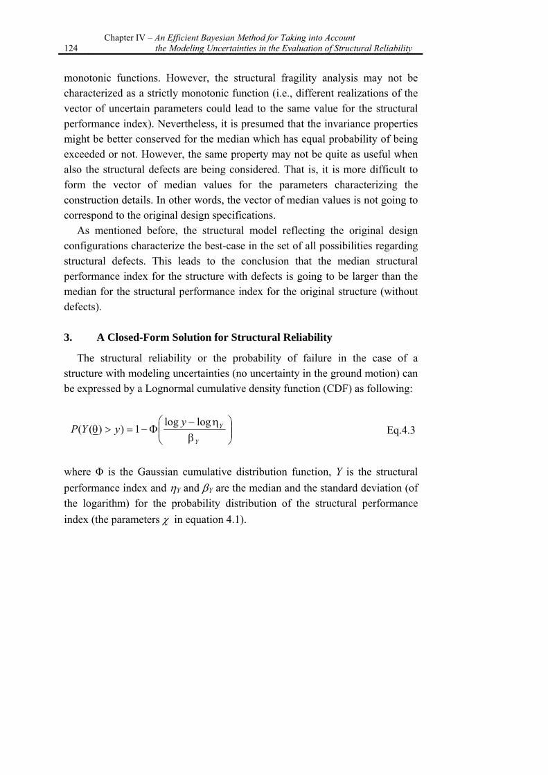
124 Chapter IV – An Efficient Bayesian Method for Taking into Account
the Modeling Uncertainties in the Evaluation of Structural Reliability
monotonic functions. However, the structural fragility analysis may not be characterized as a strictly monotonic function (i.e., different realizations of the vector of uncertain parameters could lead to the same value for the structural performance index). Nevertheless, it is presumed that the invariance properties might be better conserved for the median which has equal probability of being exceeded or not. However, the same property may not be quite as useful when also the structural defects are being considered. That is, it is more difficult to form the vector of median values for the parameters characterizing the construction details. In other words, the vector of median values is not going to correspond to the original design specifications.
As mentioned before, the structural model reflecting the original design configurations characterize the best-case in the set of all possibilities regarding structural defects. This leads to the conclusion that the median structural performance index for the structure with defects is going to be larger than the median for the structural performance index for the original structure (without defects). 3. A Closed-Form Solution for Structural Reliability
The structural reliability or the probability of failure in the case of a structure with modeling uncertainties (no uncertainty in the ground motion) can be expressed by a Lognormal cumulative density function (CDF) as following:
⎟⎟⎠
⎞⎜⎜⎝
⎛β
η−Φ−=>θ
Y
YyyYP
loglog1))(( Eq.4.3
where Φ is the Gaussian cumulative distribution function, Y is the structural performance index and ηY and βY are the median and the standard deviation (of the logarithm) for the probability distribution of the structural performance index (the parameters χ in equation 4.1).
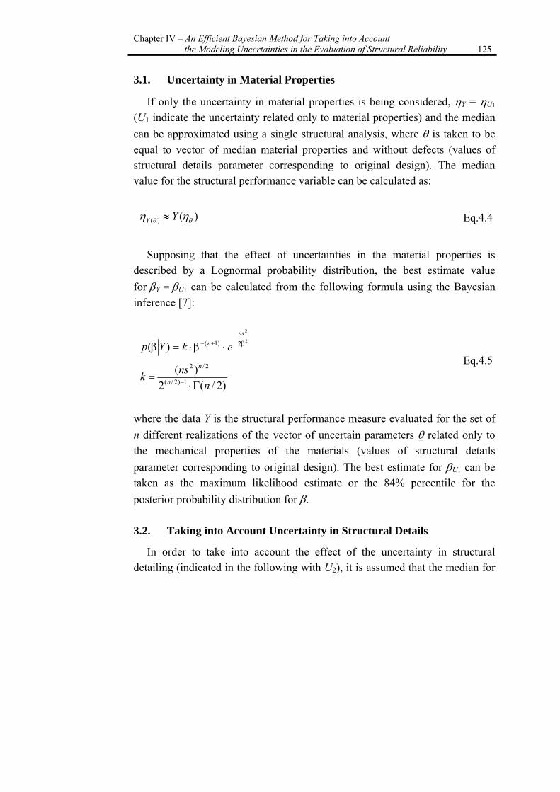
Chapter IV – An Efficient Bayesian Method for Taking into Account the Modeling Uncertainties in the Evaluation of Structural Reliability 125
3.1. Uncertainty in Material Properties
If only the uncertainty in material properties is being considered, ηY = ηU1 (U1 indicate the uncertainty related only to material properties) and the median can be approximated using a single structural analysis, where θ is taken to be equal to vector of median material properties and without defects (values of structural details parameter corresponding to original design). The median value for the structural performance variable can be calculated as:
)()( θθ ηη YY ≈ Eq.4.4
Supposing that the effect of uncertainties in the material properties is
described by a Lognormal probability distribution, the best estimate value for βY = βU1 can be calculated from the following formula using the Bayesian inference [7]:
2
2
2)1()( β−
+− ⋅β⋅=βns
n ekYp
)2/(2)(
1)2/(
2/2
nnsk n
n
Γ⋅= −
Eq.4.5
where the data Y is the structural performance measure evaluated for the set of n different realizations of the vector of uncertain parameters θ related only to the mechanical properties of the materials (values of structural details parameter corresponding to original design). The best estimate for βU1 can be taken as the maximum likelihood estimate or the 84% percentile for the posterior probability distribution for β. 3.2. Taking into Account Uncertainty in Structural Details
In order to take into account the effect of the uncertainty in structural detailing (indicated in the following with U2), it is assumed that the median for
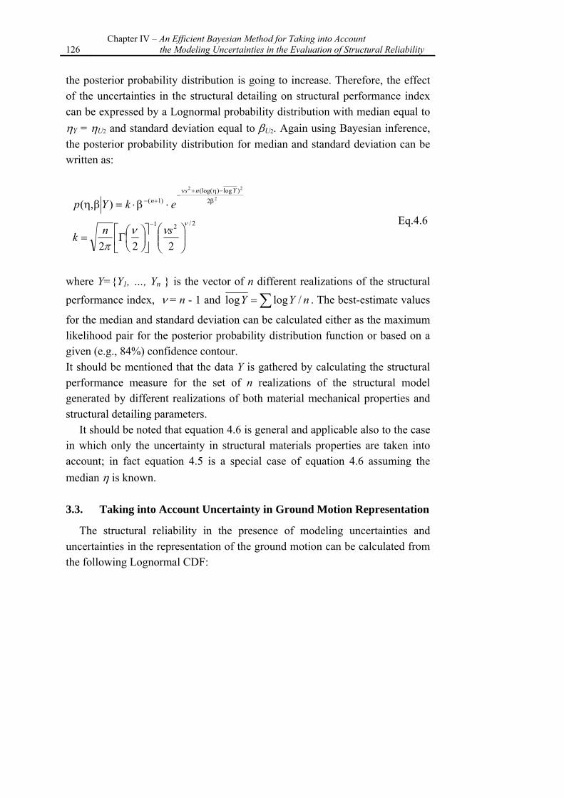
126 Chapter IV – An Efficient Bayesian Method for Taking into Account
the Modeling Uncertainties in the Evaluation of Structural Reliability
the posterior probability distribution is going to increase. Therefore, the effect of the uncertainties in the structural detailing on structural performance index can be expressed by a Lognormal probability distribution with median equal to ηY = ηU2 and standard deviation equal to βU2. Again using Bayesian inference, the posterior probability distribution for median and standard deviation can be written as:
2
22
2)log)(log(
)1(),( β
−η+ν−
+− ⋅β⋅=βηYns
n ekYp 2/21
222
ννν
π ⎟⎟⎠
⎞⎜⎜⎝
⎛⎥⎦
⎤⎢⎣
⎡⎟⎠⎞
⎜⎝⎛Γ=
−snk
Eq.4.6
where Y=Y1, …, Yn is the vector of n different realizations of the structural performance index, ν = n - 1 and ∑= nYY /loglog . The best-estimate values
for the median and standard deviation can be calculated either as the maximum likelihood pair for the posterior probability distribution function or based on a given (e.g., 84%) confidence contour. It should be mentioned that the data Y is gathered by calculating the structural performance measure for the set of n realizations of the structural model generated by different realizations of both material mechanical properties and structural detailing parameters.
It should be noted that equation 4.6 is general and applicable also to the case in which only the uncertainty in structural materials properties are taken into account; in fact equation 4.5 is a special case of equation 4.6 assuming the median η is known. 3.3. Taking into Account Uncertainty in Ground Motion Representation
The structural reliability in the presence of modeling uncertainties and uncertainties in the representation of the ground motion can be calculated from the following Lognormal CDF:
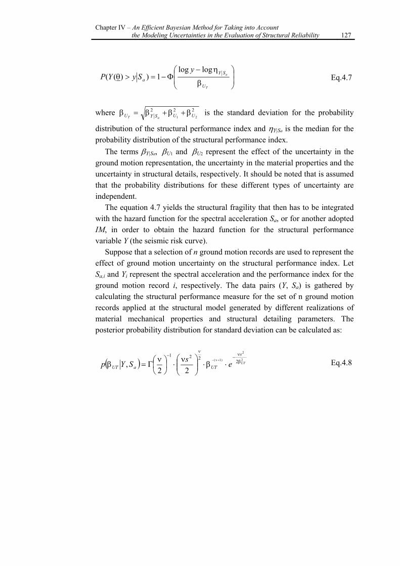
Chapter IV – An Efficient Bayesian Method for Taking into Account the Modeling Uncertainties in the Evaluation of Structural Reliability 127
⎟⎟⎠
⎞⎜⎜⎝
⎛
β
η−Φ−=>θ
T
a
U
SYa
ySyYP
loglog1))(( Eq.4.7
where 22221 UUSYU aT
β+β+β=β is the standard deviation for the probability
distribution of the structural performance index and ηY|Sa is the median for the probability distribution of the structural performance index.
The terms βY|Sa, βU1 and βU2 represent the effect of the uncertainty in the ground motion representation, the uncertainty in the material properties and the uncertainty in structural details, respectively. It should be noted that is assumed that the probability distributions for these different types of uncertainty are independent.
The equation 4.7 yields the structural fragility that then has to be integrated with the hazard function for the spectral acceleration Sa, or for another adopted IM, in order to obtain the hazard function for the structural performance variable Y (the seismic risk curve).
Suppose that a selection of n ground motion records are used to represent the effect of ground motion uncertainty on the structural performance index. Let Sa,i and Yi represent the spectral acceleration and the performance index for the ground motion record i, respectively. The data pairs (Y, Sa) is gathered by calculating the structural performance measure for the set of n ground motion records applied at the structural model generated by different realizations of material mechanical properties and structural detailing parameters. The posterior probability distribution for standard deviation can be calculated as:
( ) 2
2
)1( 2221
22, UT
s
UTaUT esSYp β
ν−
ν−
⋅β⋅⎟⎟⎠
⎞⎜⎜⎝
⎛ ν⋅⎟
⎠⎞
⎜⎝⎛ ν
Γ=β+ν−
Eq.4.8
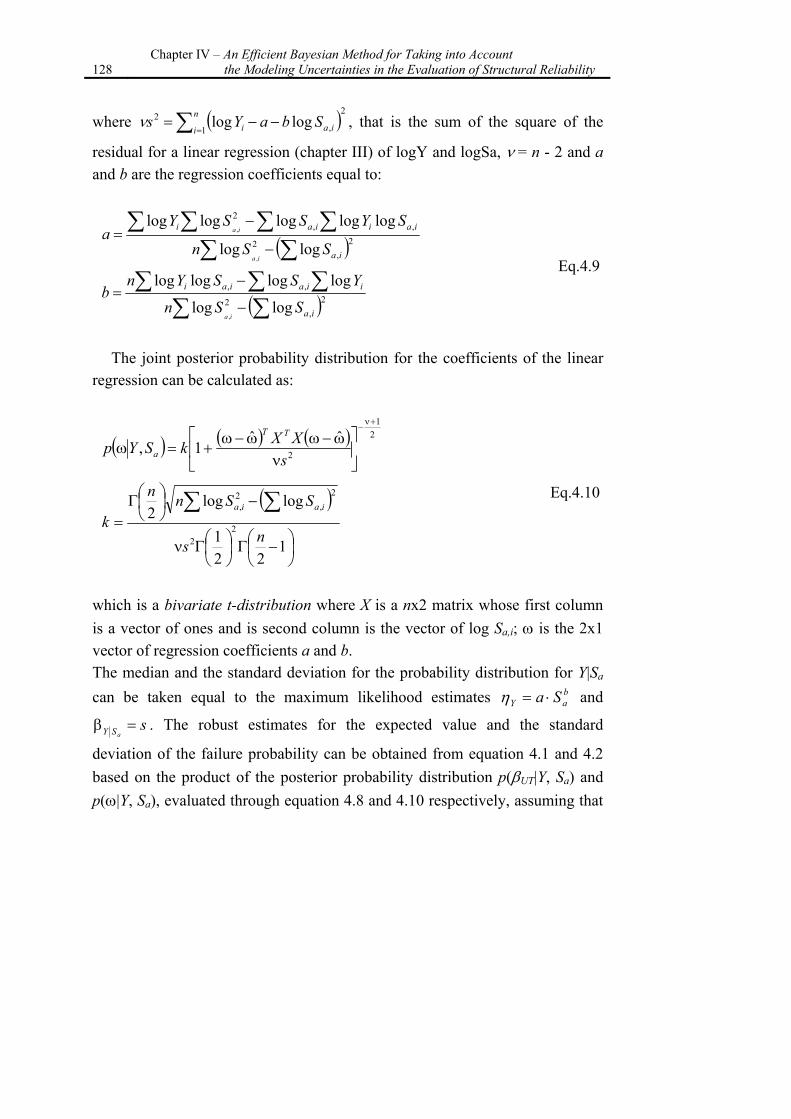
128 Chapter IV – An Efficient Bayesian Method for Taking into Account
the Modeling Uncertainties in the Evaluation of Structural Reliability
where ( )2
1 ,2 loglog∑ =
−−=n
i iai SbaYsν , that is the sum of the square of the
residual for a linear regression (chapter III) of logY and logSa, ν = n - 2 and a and b are the regression coefficients equal to:
( )∑ ∑∑ ∑ ∑ ∑
−
−= 2
,2
,,2
loglog
logloglogloglog
,
,
ia
iaiiai
SSn
SYSSYa
ia
ia
( )∑ ∑∑∑∑
−
−= 2
,2
,,
loglog
loglogloglog
, ia
iiaiai
SSn
YSSYnb
ia
Eq.4.9
The joint posterior probability distribution for the coefficients of the linear
regression can be calculated as:
( ) ( ) ( ) 21
2
ˆˆ1,
+ν−
⎥⎦
⎤⎢⎣
⎡ν
ω−ωω−ω+=ω
sXXkSYp
TT
a
( )
⎟⎠⎞
⎜⎝⎛ −Γ⎟
⎠⎞
⎜⎝⎛Γν
−⎟⎠⎞
⎜⎝⎛Γ
=∑ ∑
122
1
loglog2
22
2,
2,
ns
SSnn
kiaia
Eq.4.10
which is a bivariate t-distribution where X is a nx2 matrix whose first column is a vector of ones and is second column is the vector of log Sa,i; ω is the 2x1 vector of regression coefficients a and b. The median and the standard deviation for the probability distribution for Y|Sa can be taken equal to the maximum likelihood estimates b
aY Sa ⋅=η and
saSY =β . The robust estimates for the expected value and the standard
deviation of the failure probability can be obtained from equation 4.1 and 4.2 based on the product of the posterior probability distribution p(βUT|Y, Sa) and p(ω|Y, Sa), evaluated through equation 4.8 and 4.10 respectively, assuming that
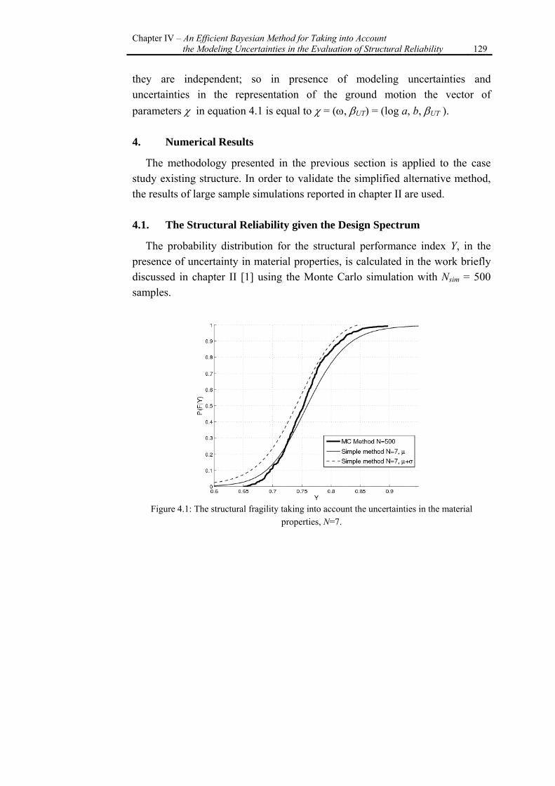
Chapter IV – An Efficient Bayesian Method for Taking into Account the Modeling Uncertainties in the Evaluation of Structural Reliability 129
they are independent; so in presence of modeling uncertainties and uncertainties in the representation of the ground motion the vector of parameters χ in equation 4.1 is equal to χ = (ω, βUT) = (log a, b, βUT ). 4. Numerical Results
The methodology presented in the previous section is applied to the case study existing structure. In order to validate the simplified alternative method, the results of large sample simulations reported in chapter II are used. 4.1. The Structural Reliability given the Design Spectrum
The probability distribution for the structural performance index Y, in the presence of uncertainty in material properties, is calculated in the work briefly discussed in chapter II [1] using the Monte Carlo simulation with Nsim = 500 samples.
Figure 4.1: The structural fragility taking into account the uncertainties in the material
properties, N=7.
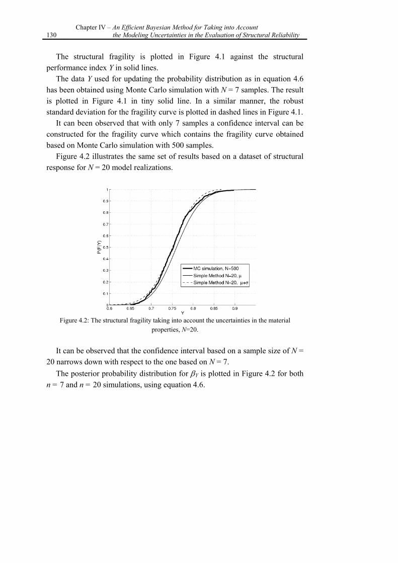
130 Chapter IV – An Efficient Bayesian Method for Taking into Account
the Modeling Uncertainties in the Evaluation of Structural Reliability
The structural fragility is plotted in Figure 4.1 against the structural performance index Y in solid lines.
The data Y used for updating the probability distribution as in equation 4.6 has been obtained using Monte Carlo simulation with N = 7 samples. The result is plotted in Figure 4.1 in tiny solid line. In a similar manner, the robust standard deviation for the fragility curve is plotted in dashed lines in Figure 4.1.
It can been observed that with only 7 samples a confidence interval can be constructed for the fragility curve which contains the fragility curve obtained based on Monte Carlo simulation with 500 samples.
Figure 4.2 illustrates the same set of results based on a dataset of structural response for N = 20 model realizations.
Figure 4.2: The structural fragility taking into account the uncertainties in the material
properties, N=20.
It can be observed that the confidence interval based on a sample size of N = 20 narrows down with respect to the one based on N = 7.
The posterior probability distribution for βY is plotted in Figure 4.2 for both n = 7 and n = 20 simulations, using equation 4.6.
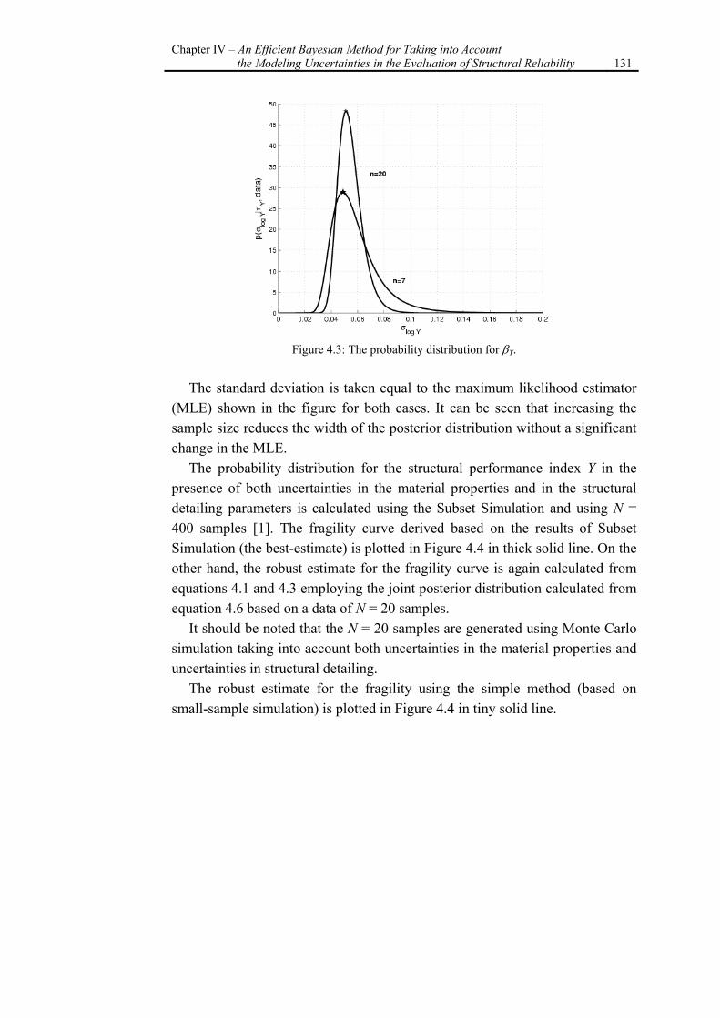
Chapter IV – An Efficient Bayesian Method for Taking into Account the Modeling Uncertainties in the Evaluation of Structural Reliability 131
Figure 4.3: The probability distribution for βY.
The standard deviation is taken equal to the maximum likelihood estimator
(MLE) shown in the figure for both cases. It can be seen that increasing the sample size reduces the width of the posterior distribution without a significant change in the MLE.
The probability distribution for the structural performance index Y in the presence of both uncertainties in the material properties and in the structural detailing parameters is calculated using the Subset Simulation and using N = 400 samples [1]. The fragility curve derived based on the results of Subset Simulation (the best-estimate) is plotted in Figure 4.4 in thick solid line. On the other hand, the robust estimate for the fragility curve is again calculated from equations 4.1 and 4.3 employing the joint posterior distribution calculated from equation 4.6 based on a data of N = 20 samples.
It should be noted that the N = 20 samples are generated using Monte Carlo simulation taking into account both uncertainties in the material properties and uncertainties in structural detailing.
The robust estimate for the fragility using the simple method (based on small-sample simulation) is plotted in Figure 4.4 in tiny solid line.
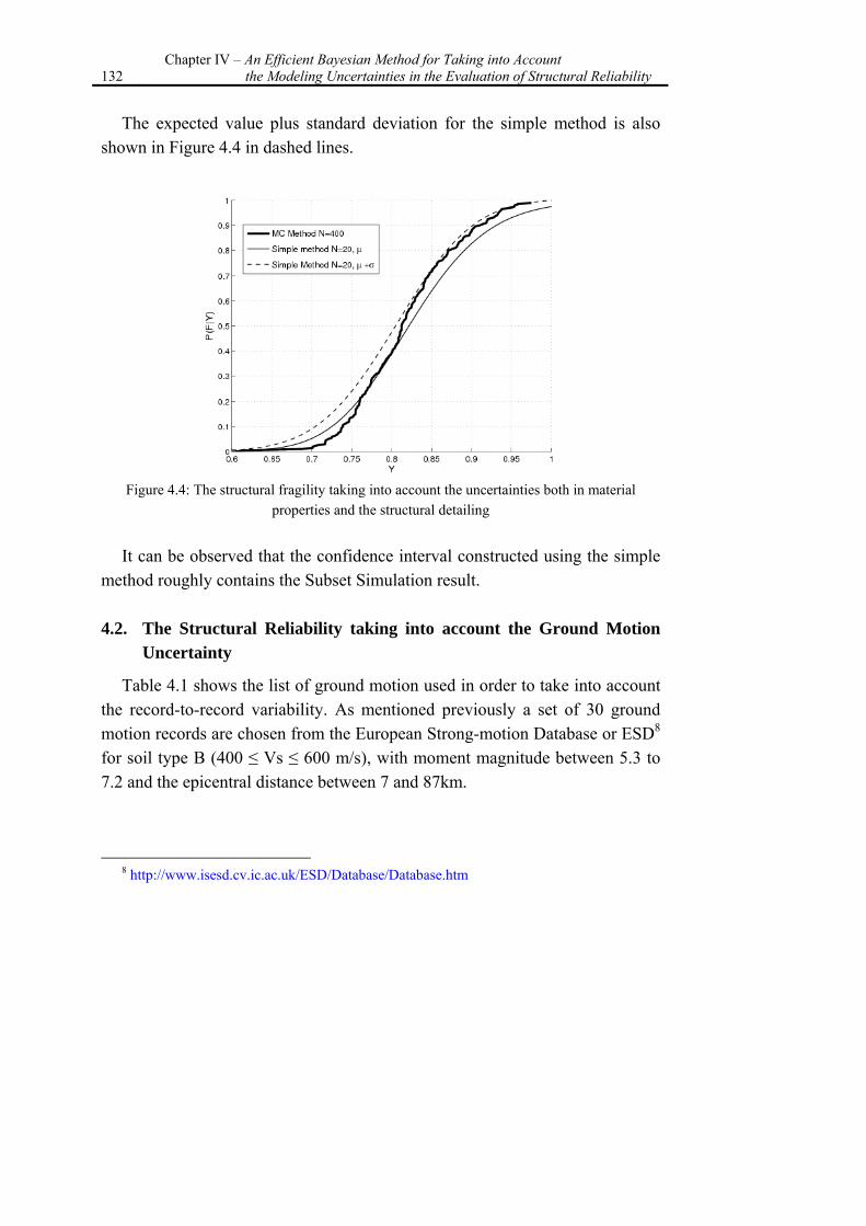
132 Chapter IV – An Efficient Bayesian Method for Taking into Account
the Modeling Uncertainties in the Evaluation of Structural Reliability
The expected value plus standard deviation for the simple method is also shown in Figure 4.4 in dashed lines.
Figure 4.4: The structural fragility taking into account the uncertainties both in material
properties and the structural detailing
It can be observed that the confidence interval constructed using the simple method roughly contains the Subset Simulation result. 4.2. The Structural Reliability taking into account the Ground Motion
Uncertainty
Table 4.1 shows the list of ground motion used in order to take into account the record-to-record variability. As mentioned previously a set of 30 ground motion records are chosen from the European Strong-motion Database or ESD8 for soil type B (400 ≤ Vs ≤ 600 m/s), with moment magnitude between 5.3 to 7.2 and the epicentral distance between 7 and 87km.
8 http://www.isesd.cv.ic.ac.uk/ESD/Database/Database.htm
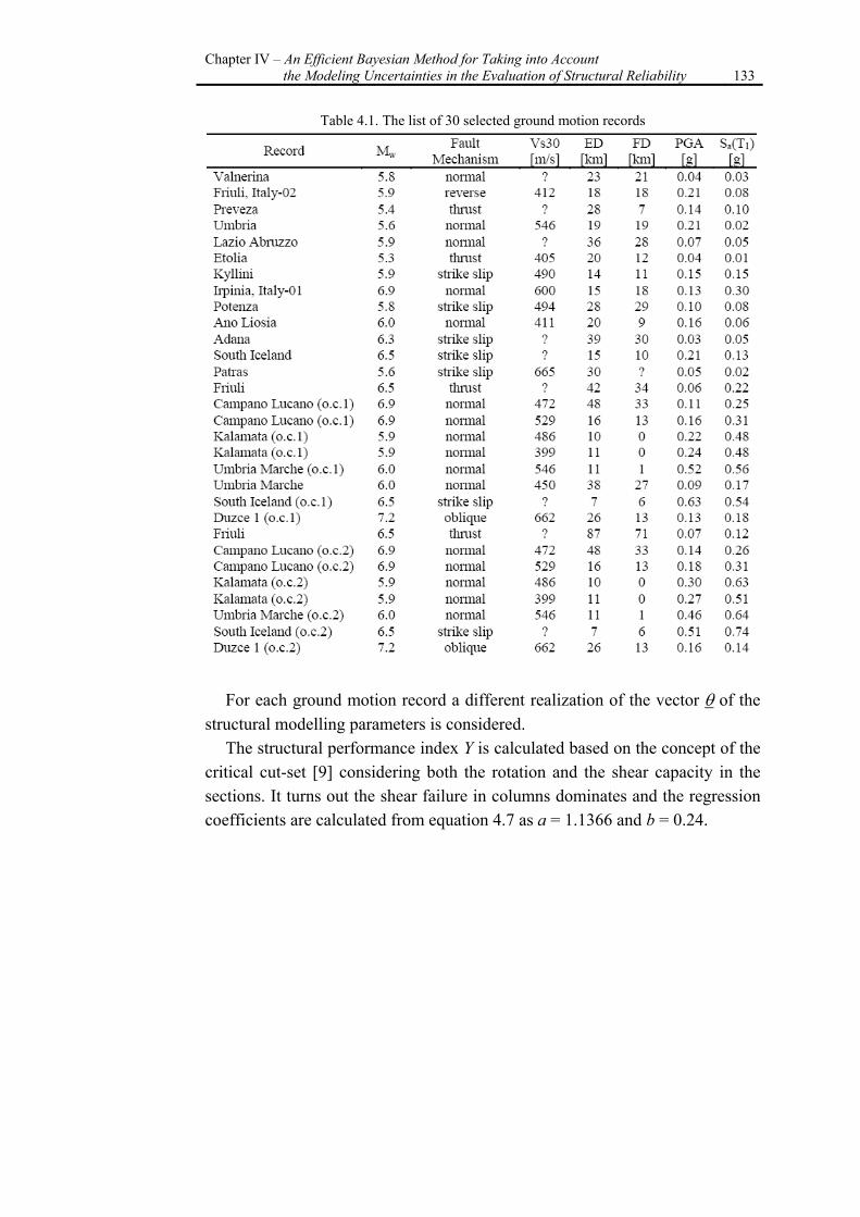
Chapter IV – An Efficient Bayesian Method for Taking into Account the Modeling Uncertainties in the Evaluation of Structural Reliability 133
Table 4.1. The list of 30 selected ground motion records
For each ground motion record a different realization of the vector θ of the structural modelling parameters is considered.
The structural performance index Y is calculated based on the concept of the critical cut-set [9] considering both the rotation and the shear capacity in the sections. It turns out the shear failure in columns dominates and the regression coefficients are calculated from equation 4.7 as a = 1.1366 and b = 0.24.
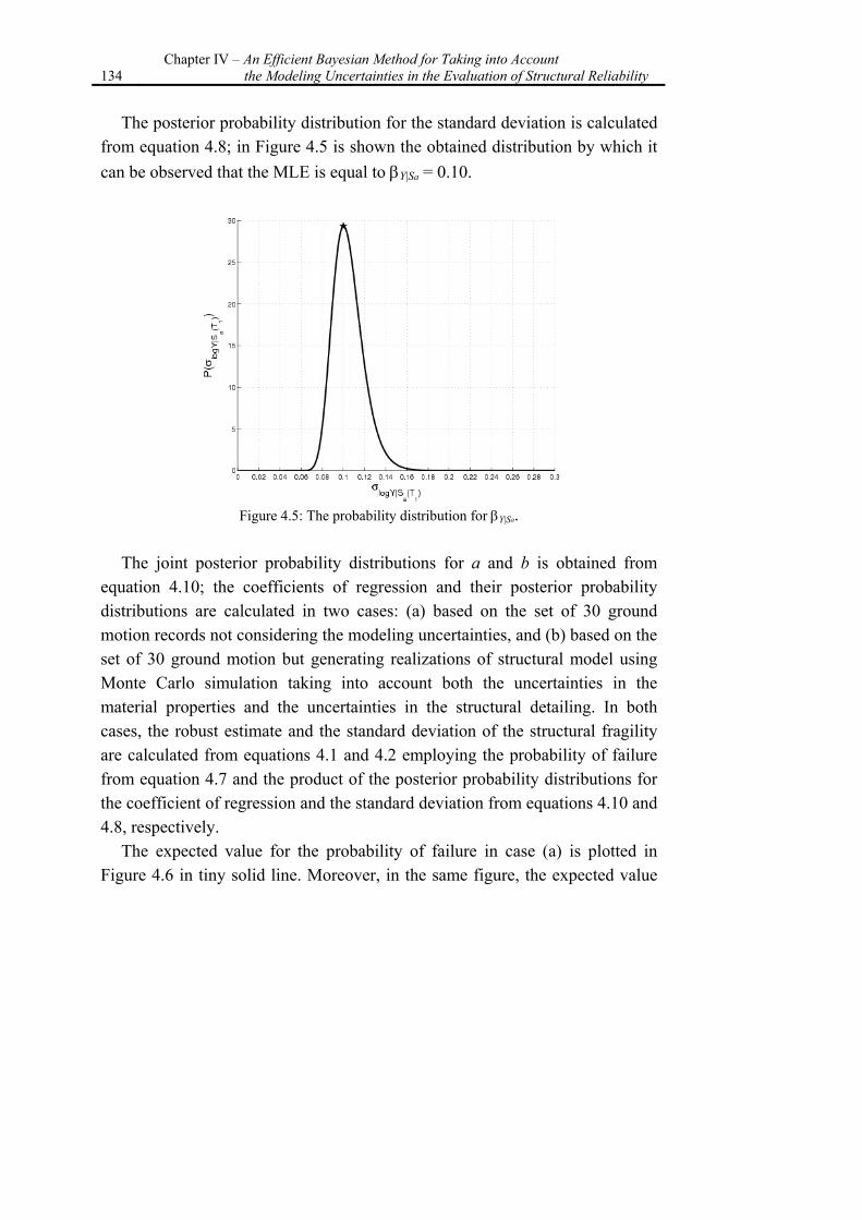
134 Chapter IV – An Efficient Bayesian Method for Taking into Account
the Modeling Uncertainties in the Evaluation of Structural Reliability
The posterior probability distribution for the standard deviation is calculated from equation 4.8; in Figure 4.5 is shown the obtained distribution by which it can be observed that the MLE is equal to βY|Sa = 0.10.
Figure 4.5: The probability distribution for βY|Sa.
The joint posterior probability distributions for a and b is obtained from
equation 4.10; the coefficients of regression and their posterior probability distributions are calculated in two cases: (a) based on the set of 30 ground motion records not considering the modeling uncertainties, and (b) based on the set of 30 ground motion but generating realizations of structural model using Monte Carlo simulation taking into account both the uncertainties in the material properties and the uncertainties in the structural detailing. In both cases, the robust estimate and the standard deviation of the structural fragility are calculated from equations 4.1 and 4.2 employing the probability of failure from equation 4.7 and the product of the posterior probability distributions for the coefficient of regression and the standard deviation from equations 4.10 and 4.8, respectively.
The expected value for the probability of failure in case (a) is plotted in Figure 4.6 in tiny solid line. Moreover, in the same figure, the expected value
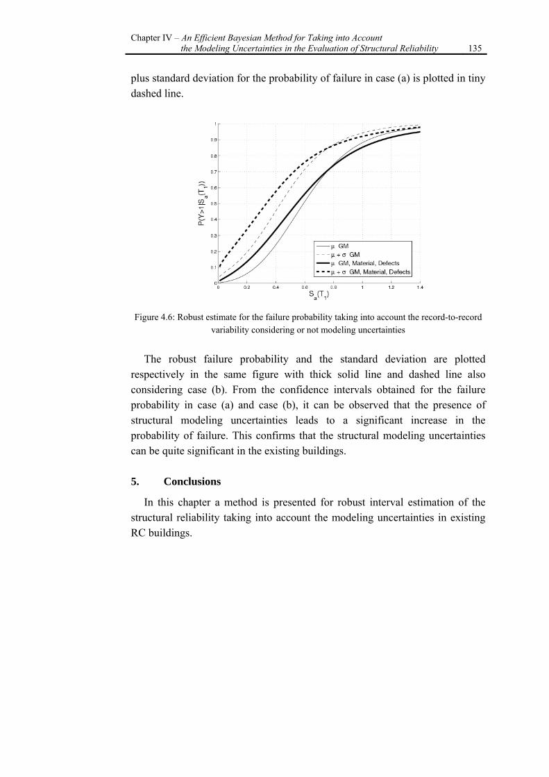
Chapter IV – An Efficient Bayesian Method for Taking into Account the Modeling Uncertainties in the Evaluation of Structural Reliability 135
plus standard deviation for the probability of failure in case (a) is plotted in tiny dashed line.
Figure 4.6: Robust estimate for the failure probability taking into account the record-to-record
variability considering or not modeling uncertainties
The robust failure probability and the standard deviation are plotted respectively in the same figure with thick solid line and dashed line also considering case (b). From the confidence intervals obtained for the failure probability in case (a) and case (b), it can be observed that the presence of structural modeling uncertainties leads to a significant increase in the probability of failure. This confirms that the structural modeling uncertainties can be quite significant in the existing buildings. 5. Conclusions
In this chapter a method is presented for robust interval estimation of the structural reliability taking into account the modeling uncertainties in existing RC buildings.
136 Chapter IV – An Efficient Bayesian Method for Taking into Account
the Modeling Uncertainties in the Evaluation of Structural Reliability
This method employs small sample structural analysis results in a Bayesian inference framework leading to posterior probability distributions for the median and standard deviation for the structural performance index.
The posterior probability distributions for the statistical parameters can be used to obtain a robust confidence interval for the probability of failure. The robust confidence interval is obtained by calculating the posterior (robust) expected value and the standard deviation of the probability of failure based on the posterior probability distribution(s).
It should be noted that the best-estimates for parameters of interest are not necessarily the maximum likelihood point estimates; they could also be interval estimates reflecting the significant uncertainty in parameter estimation due to small data sample sizes.
The results are presented in two cases, (a) for a specific representation of the ground motion uncertainty, (b) considering the record-to-record variability in ground motion.
In case (a) for which the results of extensive simulations were already available, the small-sample methods succeeded in reproducing the structural fragility curves.
In case (b), the fragility curves obtained using the small-sample inferences, make it possible to compare the influence of structural modeling uncertainties to that of the ground motion representation. They reconfirm the importance of taking into account the uncertainty both in the material properties and structural detailing in the structural reliability evaluations for an existing building.
It is demonstrated how the Bayesian framework for inference can be implemented, together with both static and dynamic analysis method, for providing confidence intervals for the structural reliability.
Chapter IV – An Efficient Bayesian Method for Taking into Account the Modeling Uncertainties in the Evaluation of Structural Reliability 137
6. References
[1] Jalayer F, Iervolino I, Manfredi G. Structural modeling uncertainties and their influence on seismic assessment of existing RC structures. Under Review Structural Safety 2008.
[2] Verderame GM, Manfredi G, Frunzio G. Le proprietà meccaniche dei calcestruzzi impiegati nelle strutture in cemento armato realizzate negli anni 60. X Congresso Nazionale \L'ingegneria Sismica in Italia", Potenza e Matera, 9-13 Settembre 2001a [in Italian].
[3] Verderame GM, Stella A, Cosenza E. Le proprietà meccaniche degli acciai impiegati nelle strutture in cemento armato realizzate negli anni '60. X Convegno Nazionale L'Ingegneria Sismica in Italia", Potenza e Matera 9-13 Settembre 2001b [in Italian].
[4] Ordinanza del Presidente del Consiglio dei Ministri (OPCM) n. 3519 (2006). Criteri per l'individuazione delle zone sismiche e la formazione e l'aggiornamento degli elenchi delle medesime zone. Gazzetta Ufficiale della Repubblica Italiana 108, 2006 (in Italian).
[5] MIN.LL.PP, DM 14 gennaio, Norme Techniche per le Costruzioni. Gazzetta Ufficiale della Repubblica Italiana, 29, 2008 (in Italian).
[6] MIN.LL.PP, DM 14 gennaio, Istruzioni per l'applicazione delle Norme Techniche delle costruzioni. Ministero della Infrastruttura, 29, 2008 (in Italian).
[7] Fajfar, P. “Capacity spectrum method based on inelastic demand spectra”, Earthquake Engineering and Structural Dynamics; 28:979–93, 1999.
[8] Jalayer F, Franchin P, Pinto PE. A scalar damage measure for seismic reliability analysis of RC frames. Earthquake Engineering and Structural Dynamics. 36:2059-2079, 2007.
[9] Ditlevsen O, Masden H. Structural Reliability Methods, June 1996; John Wiley & Sons Inc.
[10] Box GEP, Tiao GC. Bayesian Inference in Statistical Analysis. Wiley Classics Library Edition, 1992.

138 Chapter V – An Alternative Performance–Based Safety–Checking Format
Chapter V
An Alternative Performance–Based Safety–Checking Format
1. Introduction
A fully probabilistic method coupled with non-linear dynamic analysis would be the best method in order to incorporate all relevant sources of uncertainties in the assessment of existing RC structure; however pragmatism oblige the adoption of a simplified format, calibrated on the fully probabilistic method, able to put the engineer in the condition to approach the problem by incorporating the uncertainties of different nature in the assessment procedure [1].
This chapter focuses on the assessment of structural reliability for different knowledge levels employing a simple method with a format similar to the Load-Resistance Factor Design (LRFD) [2] suitable for code implementation.
The results obtained with the simple method employed herein are confronted and supported by the results obtained through probability-based methods consisting of standard Monte-Carlo simulation (chapter II) and the efficient simulation-based method (chapter IV).
For each knowledge level, the effect of tests and inspections is included by employing the Bayesian updating framework.
Chapter V – An Alternative Performance–Based Safety–Checking Format 139
The Bayesian framework for probabilistic inference seems to be a perfect vehicle for taking into account the results of tests and inspection in updating the structural model.
In chapter II has been briefly discussed a previous work by Jalayer et al. 2008 [3] in which the authors demonstrate how the simulation methods based on Bayesian updating can be used to both update the structural reliability and the probability distribution for the modeling parameters, in the presence of test and inspection results. However, the application of the simulation schemes requires a large number of structural analyses and there seems to be a need for less computationally intensive methods for updating the structural model and structural reliability. Thus, the efficient Bayesian simulation-based method for robust estimation of structural reliability, described in details in chapter IV, has been adopted. This method exploits a relatively small number of structural analyses in order to yield the robust reliability for the structure. The term robust refers to the fact that the reliability is calculated taking into account all possible structural models and their relative plausibilities.
In this chapter a probabilistic and performance-based approach is proposed as an alternative to the confidence factor approach for code-based recommendations; this format is already adopted in the American Department of Energy Guidelines DOE-1020 [4] and in SAC-FEMA guidelines [5,6,7,8].
This LRFD-like simplified approach leads to an analytic closed-form solution which compares the factored demand against factored capacity with a specified confidence level for various knowledge levels.
For seismic assessment using static analyses, an analogous formulation can be adopted which yields the structural performance parameter corresponding to a certain confidence. 2. The Knowledge Levels
Recent codes such as Eurocode 8 (EC8, [9]) seem to synthesize the effect of structural modeling uncertainties in the confidence factors (CFs) that are applied to mean material property values. The CFs are classified and tabulated as a function of discrete knowledge levels (KLs) acquired based on the results
140 Chapter V – An Alternative Performance–Based Safety–Checking Format
of specific in-situ tests and inspections. The code approach based on the CF seem to provide a level of conservatism in the assessment of existing buildings, reducing mean material property values.
The KLs are determined based on the amount of tests and inspections performed on the building (see Table I.2. of the introduction)
In this chapter four distinct knowledge levels are taken into consideration. The first knowledge level, referred to as KLo describes the state of the knowledge about the structure before the in-situ tests and inspections are performed. The other three knowledge levels KL1, KL2 and KL3 are characterized based on the Eurocode recommendations, respectively, limited, extended and comprehensive levels of knowledge. 3. The Methodology
In this section a methodology for taking into account the sources of modeling uncertainties in the probabilistic performance assessment of existing RC buildings is presented.
It should be mentioned that since this research effort mainly focuses on the code-based procedure involving the application of confidence factors, the uncertainties in the capacity models are not taken into account. This is because the Eurocode 8 [9] takes into account the uncertainty in the capacity model separately by applying a less-than-unity safety factor (γel). 3.1. Load and Resistance Factor Design Framework
The design/assessment of a structure depends upon predicted loads and the structure’s capacity to resist them. Both loads and structural capacity have various sources and levels of uncertainty.
Engineers have historically compensated for these uncertainties by using experience and subjective judgment. On the other hand, these uncertainties can be quantified using probability-based methods aimed at achieving specific performance objectives.
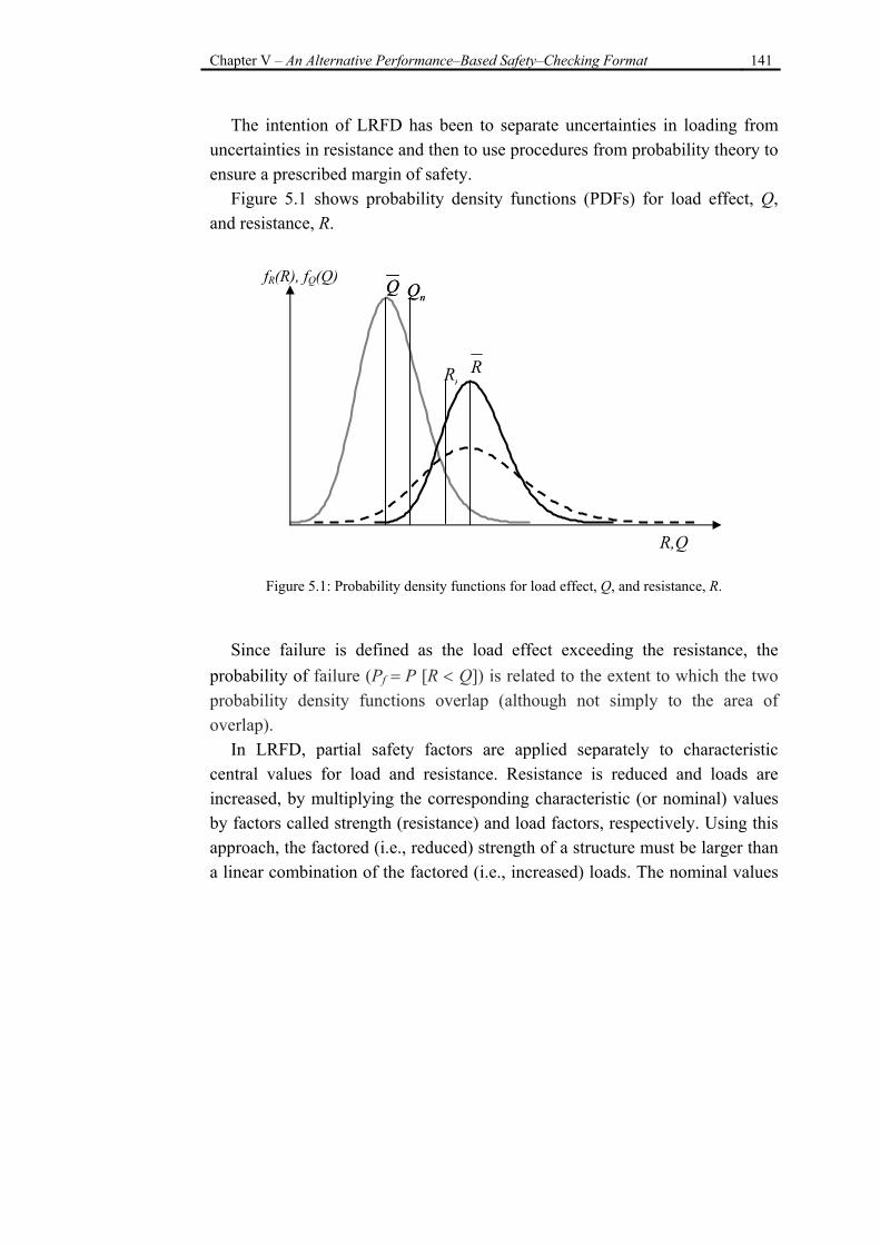
Chapter V – An Alternative Performance–Based Safety–Checking Format 141
The intention of LRFD has been to separate uncertainties in loading from uncertainties in resistance and then to use procedures from probability theory to ensure a prescribed margin of safety.
Figure 5.1 shows probability density functions (PDFs) for load effect, Q, and resistance, R.
Figure 5.1: Probability density functions for load effect, Q, and resistance, R.
Since failure is defined as the load effect exceeding the resistance, the probability of failure (Pf = P [R < Q]) is related to the extent to which the two probability density functions overlap (although not simply to the area of overlap).
In LRFD, partial safety factors are applied separately to characteristic central values for load and resistance. Resistance is reduced and loads are increased, by multiplying the corresponding characteristic (or nominal) values by factors called strength (resistance) and load factors, respectively. Using this approach, the factored (i.e., reduced) strength of a structure must be larger than a linear combination of the factored (i.e., increased) loads. The nominal values
R
Q nQ Q nQ
nR
fR(R), fQ(Q)
R,Q

142 Chapter V – An Alternative Performance–Based Safety–Checking Format
(e.g., the nominal strength, Rn) are those calculated by the specific calibrated design method and are not necessarily the means ( R and Q ).
Then, for a given structure design based on the application of resistance and load factors, the probability of failure, that is, the probability that the factored loads exceed the factored resistances, should be smaller than the prescribed value.
The importance of the LRFD format lies in the fact that the load and resistance factors are related to the uncertainty in load and resistance. Therefore, a factor of safety that is calculated as the ratio of factored resistance to factored load, already includes the effect of uncertainties (Figure 5.1), as opposed to a safety that is calculated as the ratio of median resistance to median load. 3.2. Demand and Capacity Factor Design Framework
As a proposal alternative to the confidence factor approach for code-based recommendations, a probabilistic and performance-based approach, adopted in the American Department of Energy Guidelines DOE-1020 [4] and in SAC-FEMA guidelines [5,6,7,8], is revised. This LRFD-like simplified approach leads to an analytic and closed-form solution which compares the factored demand against factored capacity.
FCFD ≤ Eq.5.1
The factored demand and capacity are respectively equal to median demand
D and median capacity C multiplied by some factors.
φγ ⋅≤⋅ CD Eq.5.2
The magnifying demand factors γ and the de-magnifying capacity factors φ
take into account all sources of uncertainty, such as record-to-record (ground
Chapter V – An Alternative Performance–Based Safety–Checking Format 143
motion) variability, structural modeling uncertainty and the uncertainty in the capacities. This approach, that is also known as the Demand and Capacity Factor Design (DCFD) [10] for its similarity with the LRFD (AISC, LRFD Code) [2], takes into account the overall effect of the various types of uncertainties on a global structural performance parameter.
The alternative proposals discussed herein can all be implemented in order to estimate the parameters within the DCFD framework for safety checking of existing buildings for various knowledge levels.
In this section the adopted DCFD format is briefly described starting from the most general case that also includes the uncertainty in ground motion representation employing non-linear dynamic analysis, in particular the cloud method presented in chapter III. However an alternative performance-based safety-checking format is also presented herein employing non-linear static analysis. 3.2.1. DCFD and PBEE Frameworks
Adopting the probabilistic performance-based assessment described in chapter II (PBEE), a probabilistic performance objective can be expressed by ensuring that the MAF (mean annual frequency) λLS of structural demand D reaching or exceeding structural capacity CLS for a limit state is smaller than or equal to a tolerable annual frequency P0:
( ) 0PCD LSLS ≤>= λλ Eq.5.3
where λLS is also referred to, more briefly, as the limit state probability and/or failure probability9. It should be noted that the demand and capacity terms appearing in the performance objective are global variables.
9 For an event with very small probability of occurrence, such as a strong earthquake, the
numerical value of MAF of occurrence and the probability of occurrence in one year are very
close.
144 Chapter V – An Alternative Performance–Based Safety–Checking Format
In the framework of DCFD the performance objective in equation 5.3 is represented in the following form:
FCPFD ≤)( 0 Eq.5.4
where FD(P0) is the factored demand at the allowable probability level P0 and FC is the factored capacity [11].
The structural performance parameter is the one adopted in all the other chapters, that is the critical demand to capacity ratio denoted as Y. As stated previously, this ratio assumes the value of unity on the verge of the limit state function. By adopting this structural performance parameter, the structural reliability can be expressed as the probability that Y assumes a value greater than unity:
( )1>= YPPf
Eq.5.5
Introducing the critical demand to capacity ratio Y, the performance
objective in equation 5.3 is expressed as:
( ) 01 PY ≤>λ Eq.5.6
Consequently the performance objective in equation 5.4 is expressed as:
1)( 0 ≤PFY Eq.5.7
Chapter V – An Alternative Performance–Based Safety–Checking Format 145
Under the assumption that: 1) the spectral acceleration hazard is described as a power-law function of
the spectral acceleration level (the chosen IM):
( ) kaaS SkS
a
−⋅= 0λ Eq.5.8a
2) the critical demand to capacity ratio can be expressed as:
aa SYSYY || εη ⋅= Eq.5.8b
where it is assumed that the median is a power-law function of the spectral acceleration level ( b
aSY Saa
⋅=|η ) and that aSY |ε is described by a
unit-median Lognormal PDF with fractional standard deviation equal to
aSY |β .
than the performance objective in equation 5.7 can be derived as:
12
0|0
21
|≤⋅
PaSY
Pa
bk
SYe
βη
Eq.5.9
where 0| P
aSYη and 0| P
aSYβ are median and fractional standard deviation of the
critical demand to capacity ratio at a spectral acceleration equal to 0PaS which
has mean annual frequency of exceedance equal to P0. It should be noted that the expression in the first term of the equation 5.9 is
based on a property of the lognormal variables, where the expected value of a lognormal variable is equal to its median times the exponential of half of the squared standard deviation [12].
The performance objective in equation 5.9 compares the factored critical demand to capacity ratio at allowable probability P0 against unity.
146 Chapter V – An Alternative Performance–Based Safety–Checking Format
A single variable εUC is employed to represent the (global) effect of component modelling uncertainties on the fragility curve and it is assumed that εUC is Lognormal with unit median and fractional standard deviation βUC.
An extended formulation of the DCFD format in the presence of structural modelling uncertainties can be derived by assuming that the median critical demand to capacity ratio can be expressed as follows:
UCSYSY UCaaεηη ε ⋅= =1,|| Eq.5.10
where 1,| =UCaSY εη is the median critical demand to capacity ratio for a given Sa
and under the assumption that there is no capacity modelling uncertainty. It should be noted that it is assumed that the uncertain variable εUC
representing the global effect of modelling uncertainty is independent of the Sa level.
The DCFD performance objective in terms of the critical demand to capacity ratio in the presence of capacity modelling uncertainty can be derived as:
122
0|0
21
21
,|≤⋅⋅
UCPaSY
UCPa
bk
bk
SYee
ββ
εη
Eq.5.11
3.2.2. Non-Linear Static Analysis
In the case of static analyses, the capacity spectrum method (CSM) [13] is used to obtain the global demand to capacity ratio (Appendix C). Moreover, at the onset of the limit state, the shear capacity of the structural components is also verified by calculating the shear demand to capacity ratio for the structural components (Appendix E). The overall structural performance parameter is finally taken as the larger between the critical shear component demand to capacity ratio and the overall demand to capacity ratio derived from CSM.
Chapter V – An Alternative Performance–Based Safety–Checking Format 147
The expected value for the critical demand to capacity ratio can be calculated from the following (assuming that Y is described by a Lognormal distribution):
12
21
≤⋅ηβ Y
eY Eq. 5.12
where ηY is the median and βY is the standard deviation of the logarithm for the probability distribution for the structural performance parameter Y. The parameter βY represents the overall effect of uncertainties on the probability distribution for the structural performance parameter.
In other words, the inequality in equation 5.12 is checks whether the expected (mean) value for the structural performance parameter is less than or equal to unity. Alternatively, one can calculate a given percentile %x of the structural performance parameter Y and check to see whether it is less than or equal to unity:
1)(1
≤⋅η βΦ−Yx
Y e Eq. 5.13
where Φ-1(x) is the inverse Gaussian cumulative density function (CDF) for percentile x. 3.2.3. Non-Linear Dynamic Analysis
In the case of dynamic analyses, the cut-set [14] concept in reliability theory is employed to find the critical component demand to capacity ratio that takes the structure closer to the onset of the limit state. This critical demand to capacity ratio corresponds to the strongest component of the weakest structural mechanism [11]:
min max ljl j
lj
DY
C= Eq. 5.14
148 Chapter V – An Alternative Performance–Based Safety–Checking Format
where l is the structural mechanism index considered and j is the component index within lth mechanism. In this case the mechanisms considered involve the ultimate chord rotation in the components, the formation of global mechanisms (e.g., soft story and beam mechanisms) and the component shear capacity.
When the uncertainty in the ground motion representation (the record-to-record variability) is considered, the DCFD formulation is expressed as:
1)()(
21 2
|2
≤⋅ηβ+β UCaSY
bk
oY eP Eq. 5.15
where Po is an acceptable threshold for structural failure probability and ηY(Po) is the median structural performance parameter corresponding to the acceptable probability Po. The terms βY|Sa and βUC represent the effect of record-to-record (Ground Motion) variability and structural modeling uncertainties, respectively, on the total dispersion in the structural performance parameter given spectral acceleration. In the same manner as the static case, the inequality in equation 5.7 can be verified with a certain %x confidence:
2 1 2 2| |1
( )2( ) Y Sa Y S UCa
kxb
Y oP e eβ β βη
−−Φ +⋅ ≤ Eq. 5.16
where Φ-1(x) is the inverse Gaussian cumulative density function (CDF) for percentile x. 3.3. Characterization of the Uncertainties for KL0
It is assumed that the vector θ represents all the uncertain parameters considered in the problem.
Typically, the uncertainties present in a seismic assessment problem can be classified in different groups, namely, the uncertainties in the representation of the ground motion, the modeling uncertainties, associated with the structural finite element model and the component capacity models, and the uncertainties
Chapter V – An Alternative Performance–Based Safety–Checking Format 149
in the structural modeling parameters. As stated in the previous chapters this work focuses on the uncertainty in the structural modelling parameters related to the available information on the characteristics of existing buildings. This is the type of uncertainty that is believed to be addressed implicitly by the application of confidence factors. Two groups of structural modeling uncertainties are considered, the uncertainty in the mechanical property of materials and the uncertainty in the structural construction details. 3.3.1. Materials
The parameters identifying the prior probability distributions for the material mechanical properties (concrete strength and the steel yielding force) have been based on the values typical of the post world-war II construction in Italy [15,16]. The parameters that are used to define the Lognormal probability distributions for the material properties are the same adopted in the previous chapter and reported in chapter II, Table 2.2. 3.3.2. Structural Details
One of the main characteristics of the construction details is that possible deviations from the original configurations are mostly taken into account in those cases leading to undesirable effects. This justifies why the uncertainties related to construction details are usually referred to as the structural defects.
The prior probability distributions for the structural detailing parameters can be defined based on qualitative prior information coming from expert judgment or based on ignorance in the extreme case [3]. Table 5.1 shows (for illustrative purpose only) the example specifications used to construct the prior probability distributions for the structural detailing parameters.
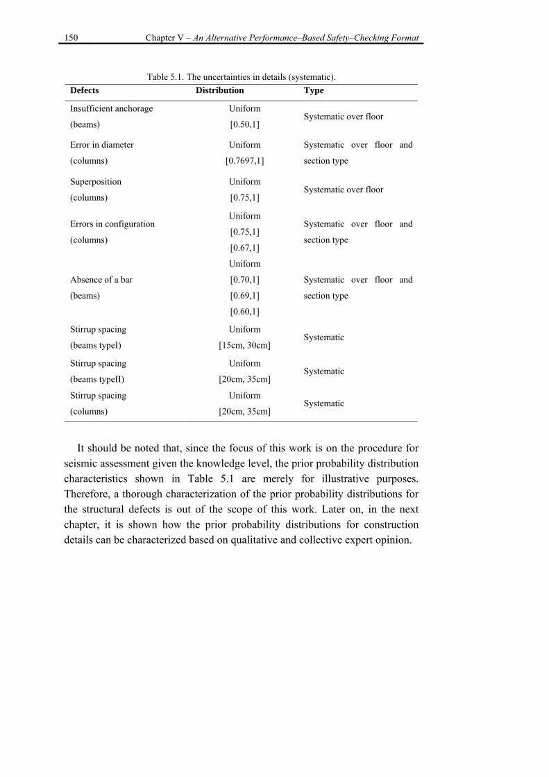
150 Chapter V – An Alternative Performance–Based Safety–Checking Format
Table 5.1. The uncertainties in details (systematic). Defects Distribution Type
Insufficient anchorage
(beams)
Uniform
[0.50,1] Systematic over floor
Error in diameter
(columns)
Uniform
[0.7697,1]
Systematic over floor and
section type
Superposition
(columns)
Uniform
[0.75,1] Systematic over floor
Errors in configuration
(columns)
Uniform
[0.75,1]
[0.67,1]
Systematic over floor and
section type
Absence of a bar
(beams)
Uniform
[0.70,1]
[0.69,1]
[0.60,1]
Systematic over floor and
section type
Stirrup spacing
(beams typeI)
Uniform
[15cm, 30cm] Systematic
Stirrup spacing
(beams typeII)
Uniform
[20cm, 35cm] Systematic
Stirrup spacing
(columns)
Uniform
[20cm, 35cm] Systematic
It should be noted that, since the focus of this work is on the procedure for seismic assessment given the knowledge level, the prior probability distribution characteristics shown in Table 5.1 are merely for illustrative purposes. Therefore, a thorough characterization of the prior probability distributions for the structural defects is out of the scope of this work. Later on, in the next chapter, it is shown how the prior probability distributions for construction details can be characterized based on qualitative and collective expert opinion.
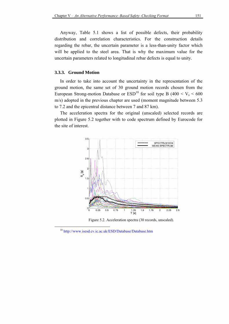
Chapter V – An Alternative Performance–Based Safety–Checking Format 151
Anyway, Table 5.1 shows a list of possible defects, their probability distribution and correlation characteristics. For the construction details regarding the rebar, the uncertain parameter is a less-than-unity factor which will be applied to the steel area. That is why the maximum value for the uncertain parameters related to longitudinal rebar defects is equal to unity.
3.3.3. Ground Motion
In order to take into account the uncertainty in the representation of the ground motion, the same set of 30 ground motion records chosen from the European Strong-motion Database or ESD10 for soil type B (400 < Vs < 600 m/s) adopted in the previous chapter are used (moment magnitude between 5.3 to 7.2 and the epicentral distance between 7 and 87 km).
The acceleration spectra for the original (unscaled) selected records are plotted in Figure 5.2 together with to code spectrum defined by Eurocode for the site of interest.
Figure 5.2. Acceleration spectra (30 records, unscaled).
10 http://www.isesd.cv.ic.ac.uk/ESD/Database/Database.htm
152 Chapter V – An Alternative Performance–Based Safety–Checking Format
3.4. Updating the Probability Distribution
The probability distributions for the structural modeling parameters can be updated employing the Bayesian framework for inference.
It is assumed that the material properties are homogeneous across each floor or construction zone. Therefore, the material property value assigned to each floor can be thought of as an average of the material property values across the floor/zone in question. The results of tests and inspections for each floor can be used to update the probability distribution for the mean material property across the floor. Figure 5.3 illustrates an example where the test results for concrete strength have all verified the nominal value (fc = 165 kg/cm2) for different levels of knowledge. It can be observed that the updated curve has the same median but has its dispersion reduced as the amount of data increases. In the following the updating procedure for the concrete strength fc is demonstrated; however, the exact same procedure is applied for steel yielding strength fy.
Let : 1: iD D i N= = denote the set of data available for the concrete
strength for a given construction zone. Assuming that the data measurements contain no errors11, the updated probability distribution for mean concrete strength across the floor can be calculated using the Bayes formula:
( | ) ( )( | )( | ) ( )
c cc
c c c
p D f p fp f Dp D f p f df
=∫
Eq. 5.17
11 The consideration of measurement errors can also be implemented in the Bayesian
updating procedure. For example for a given data measurement denoted by D , the probability distribution for D given the exact value D can be denoted by ˆ( | )p D D . Therefore, the
likelihood for data measurement D given the mean concrete strength fc is known can be calculated as: ˆ ˆ( | ) ( | ) ( | )c cp D f p D D p D f dD= ∫ , (assuming that the measurement error does not
depend on fc).
Chapter V – An Alternative Performance–Based Safety–Checking Format 153
where, p(fc) denotes the prior probability distribution for the mean concrete strength across the construction zone. For example, in this case it can refer to the characterization of the uncertainty in concrete strength before the tests are conducted for the knowledge level KLo; that is the lognormal distribution described in Table 5.3.
Table 5.3. Probabilistic characterization of the mechanical property of RC. Variable Distribution Mean [kg/cm2] COV
fy LogNormal 165 0.15 fc LogNormal 3200 0.08
Moreover, assuming that the data are independent, the likelihood p(D|fc) can be written as:
1
( | ) ( | )N
c i ci
p D f p D f=
= ∏ Eq. 5.18
The likelihood functions ( | )i cp D f are also assumed to be lognormal
probability distribution with median value equal to fc and standard deviation of the logarithm equal to the value tabulated in Table 5.3.
Figure 5.3 illustrates the probability distribution of the mean concrete strength value across the construction zone for the knowledge levels, KLo, KL1, KL2 and KL3 based on the extreme hypothesis that all the test results confirm the nominal (median) value.
It should be mentioned that such an extreme hypothesis is considered for the purpose of parameter studies on the effect of test results. Otherwise, the methodology is general with respect to the outcome of the test results. It can be observed from the figure that standard deviation for the updated probability distribution for each knowledge level decreases across increasing knowledge levels while the median value remains invariant.
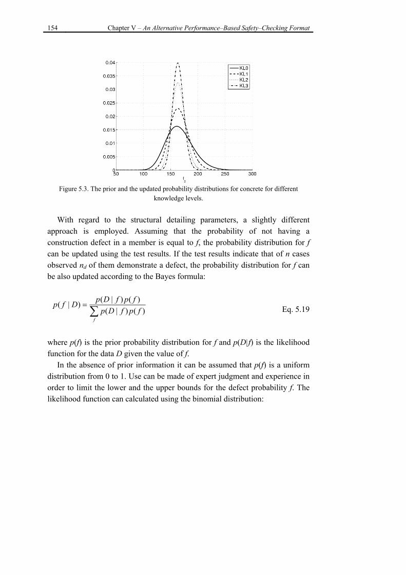
154 Chapter V – An Alternative Performance–Based Safety–Checking Format
Figure 5.3. The prior and the updated probability distributions for concrete for different
knowledge levels. With regard to the structural detailing parameters, a slightly different
approach is employed. Assuming that the probability of not having a construction defect in a member is equal to f, the probability distribution for f can be updated using the test results. If the test results indicate that of n cases observed nd of them demonstrate a defect, the probability distribution for f can be also updated according to the Bayes formula:
∑=
ffpfDp
fpfDpDfp)()|(
)()|()|( Eq. 5.19
where p(f) is the prior probability distribution for f and p(D|f) is the likelihood function for the data D given the value of f.
In the absence of prior information it can be assumed that p(f) is a uniform distribution from 0 to 1. Use can be made of expert judgment and experience in order to limit the lower and the upper bounds for the defect probability f. The likelihood function can calculated using the binomial distribution:
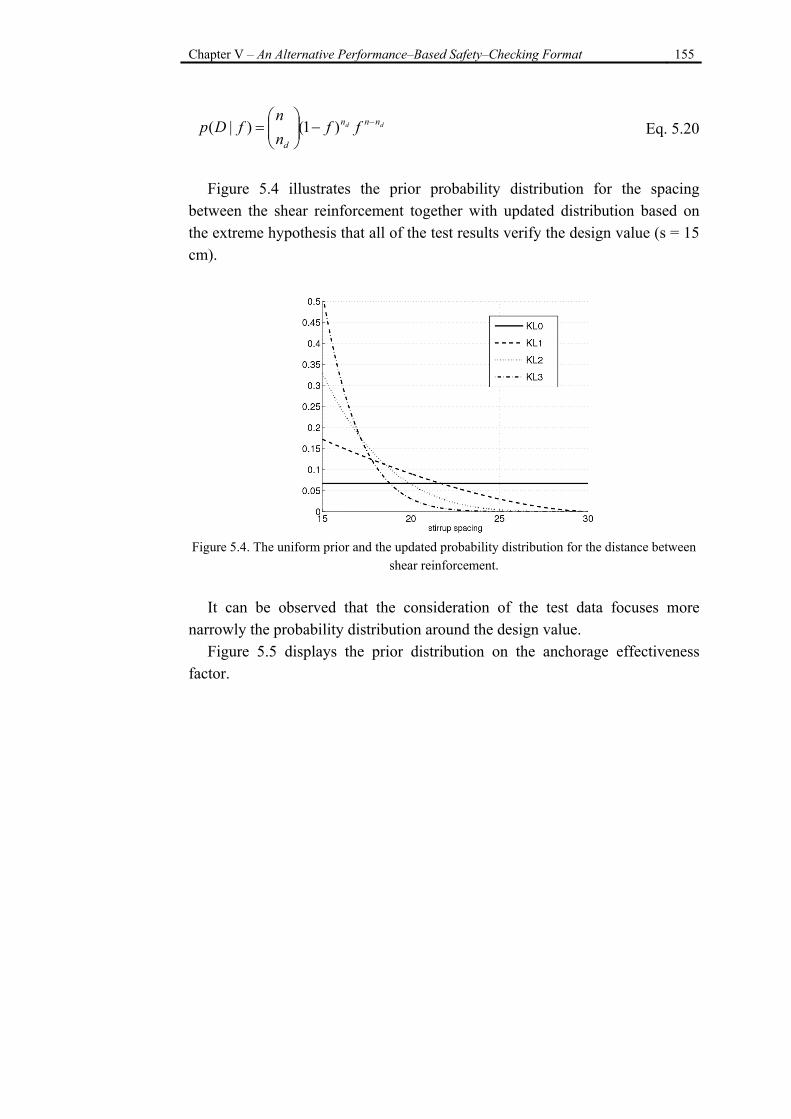
Chapter V – An Alternative Performance–Based Safety–Checking Format 155
dd nnn
d
ffnn
fDp −−⎟⎟⎠
⎞⎜⎜⎝
⎛= )1()|( Eq. 5.20
Figure 5.4 illustrates the prior probability distribution for the spacing
between the shear reinforcement together with updated distribution based on the extreme hypothesis that all of the test results verify the design value (s = 15 cm).
Figure 5.4. The uniform prior and the updated probability distribution for the distance between
shear reinforcement.
It can be observed that the consideration of the test data focuses more narrowly the probability distribution around the design value.
Figure 5.5 displays the prior distribution on the anchorage effectiveness factor.
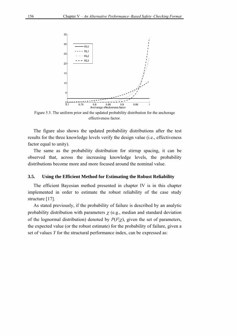
156 Chapter V – An Alternative Performance–Based Safety–Checking Format
Figure 5.5. The uniform prior and the updated probability distribution for the anchorage
effectiveness factor.
The figure also shows the updated probability distributions after the test results for the three knowledge levels verify the design value (i.e., effectiveness factor equal to unity).
The same as the probability distribution for stirrup spacing, it can be observed that, across the increasing knowledge levels, the probability distributions become more and more focused around the nominal value. 3.5. Using the Efficient Method for Estimating the Robust Reliability
The efficient Bayesian method presented in chapter IV is in this chapter implemented in order to estimate the robust reliability of the case study structure [17].
As stated previously, if the probability of failure is described by an analytic probability distribution with parameters χ (e.g., median and standard deviation of the lognormal distribution) denoted by P(F|χ), given the set of parameters, the expected value (or the robust estimate) for the probability of failure, given a set of values Y for the structural performance index, can be expressed as:
Chapter V – An Alternative Performance–Based Safety–Checking Format 157
[ ( | )] ( | ) ( | )E P F D P F p D dχ χ χΩ
= ∫ Eq. 5.21
where p(χ |D) is the posterior probability distribution for the set of parameters χ given the data D and Ω is the space of possible values for χ. In a similar way, the robust variance for the probability of failure can be calculated as:
22)|( )]|([])|([ DFPEDFPEDFP −=σ Eq. 5.22
In particular, the structural reliability or the probability of failure in the case of a structure with modeling uncertainties (no uncertainty in the ground motion) can be expressed by a Lognormal CDF:
⎟⎟⎠
⎞⎜⎜⎝
⎛β
η−Φ−=>θ
Y
YyyYP loglog1))(( Eq.5.23
in which the vector of parameter χ, indicated in equation 5.21 is formed by ηY , βY. Using Bayesian inference, the posterior probability distribution for median and standard deviation based on data Y can be written as [18]:
2/21
2
22)1(
2)2/(
2
)2
)log(logexp()|,(
ννν
π
βηνββη
⎟⎟⎠
⎞⎜⎜⎝
⎛Γ=
−+−=
−
+−
snk
YnskYPY
YnYYY
Eq. 5.24
where Y=Y1, …, Yn is the vector of n different realizations of the structural performance index, ν=n-1, Ylog is the mean value for logY and ns2 is sum of
158 Chapter V – An Alternative Performance–Based Safety–Checking Format
the squares of the deviations from the mean value. The expected value and the standard deviation for the probability of failure can be calculated from equations 5.21 and 5.22 based on the posterior probability distribution p(χ|D) = p(ηY, βY|Y) in equation 5.24. Otherwise, the best-estimate values for the median and standard deviation can be calculated either as the maximum likelihood pair for the posterior probability distribution function or based on a given (e.g., 84%) confidence level.
The structural reliability in the presence of modeling uncertainties and uncertainties in the representation of the ground motion can be calculated from the Lognormal CDF:
UCSYUT
UT
SYa
a
ay
SyYP
2|
22
|loglog1)|)((
βββ
βη
θ
+=
⎟⎟⎠
⎞⎜⎜⎝
⎛ −Φ−=>
Eq. 5.25
where ηY|Sa is the median for the probability distribution of the structural performance index and βUT is the standard deviation for the probability distribution of the structural performance index. The terms βY|Sa and βUC represent the effect of the uncertainty in the ground motion representation, the uncertainty in the material properties and the structural details, respectively. It should be noted that equation 5.25 yields the structural fragility; after integrating it with the hazard function for the spectral acceleration, or for another adopted IM, the hazard function for the structural performance variable Y (the seismic risk curve) can be obtained.
Suppose that a selection of n ground motion records are used to represent the effect of ground motion uncertainty on the structural performance index. Let Sa,i and Yi represent the spectral acceleration and the performance index for the ground motion record i, respectively. The posterior probability distribution for standard deviation can be calculated as:
Chapter V – An Alternative Performance–Based Safety–Checking Format 159
/ 22 21 ( 1)
2( | ) ( / 2) exp( )2 2UT UT
UT
s sP Yν
νν νβ ν ββ
− − +⎛ ⎞ −= Γ ⎜ ⎟
⎝ ⎠ Eq. 5.26
The data pairs (Y, Sa) are gathered by calculating the structural performance
measure for the set of n ground motion records applied at the structural model generated by different realizations of material mechanical properties and structural detailing parameters. The terms νs2 is equal to the sum of the square of the residuals for a linear regression of logY on logSa and a and b are the regression coefficients. The joint posterior probability distribution for the coefficients of the linear regression ω = (log a, b) can be calculated as:
⎟⎠⎞
⎜⎝⎛ −Γ⎟
⎠⎞
⎜⎝⎛Γ
−⎟⎠⎞
⎜⎝⎛Γ
=
⎥⎦
⎤⎢⎣
⎡ −−+=
∑∑
+−
122
1
)log(log2
)ˆ()ˆ(1),|(
22
2,,
2
21
2
ns
SSnn
k
sXXkSYP
iaia
TT
a
ν
νωωωωω
ν
Eq. 5.27
which is a bivariate t-distribution where X is a 2n× matrix whose first column is a vector of ones and its second column is the vector of log Sa,i and ω is the 2 1× vector of regression coefficients log a and b. The median and the standard deviation for the probability distribution for Y|Sa can be taken equal to the maximum likelihood estimates ηY = aSa
b and βY|Sa=s. The robust estimates for the expected value and the standard deviation of the failure probability can be obtained from equations 5.21 and 5.2 by substituting the product of the posterior probability distributions p(ω|Y,Sa) and p(βUT|Y,Sa) in equations 5.27 and 5.26, assuming they are independent. χ=(ω , βUT )= (log a, b, βUT).
160 Chapter V – An Alternative Performance–Based Safety–Checking Format
4. Application to the Case-Study Structure
The methodology presented in this section is applied to the case study existing structure. 4.1. Non-Linear Static Analysis
When only the structural modeling uncertainties are considered, the definition of structural capacity in this work is based on the limit state of severe damage as proposed by the Italian Code [19,20,21]. That is, the onset of critical behavior in the first element, characterized by member chord rotations larger than 3/4th of the corresponding ultimate chord rotation capacity. The structural demand is characterized by the intersection of the code-based inelastic design spectrum and the static pushover curve transformed into that of the equivalent SDOF system [13] (Appendix C). As an index for the global structural performance, the ratio of structural demand to capacity is used [11]. The component yield rotation, ultimate rotation and shear capacities are calculated according to the new Italian Unified Code [20,21] (Appendices B and E). 4.1.1. Calculation of the Structural Fragility
The structural fragility curve for the structure under study can be calculated by employing the efficient Bayesian method described above based on the structural performance parameter for static analyses for a set of 20 Monte Carlo (MC) realizations of the structural model. These realizations take into account the uncertainties in the material properties and the structural defects. The probability distributions for the uncertain parameters are updated according to the increasing knowledge levels. Thus, for each knowledge level, the 20 realizations of the structural model are generated from the (updated) probability distributions corresponding to the KL’s and based on the results of tests and inspections. Since the results of tests and inspections available for the structure in question did not exactly match the EC8 [9] criteria, the test results used herein are simulated assuming that all the inspections performed verify the
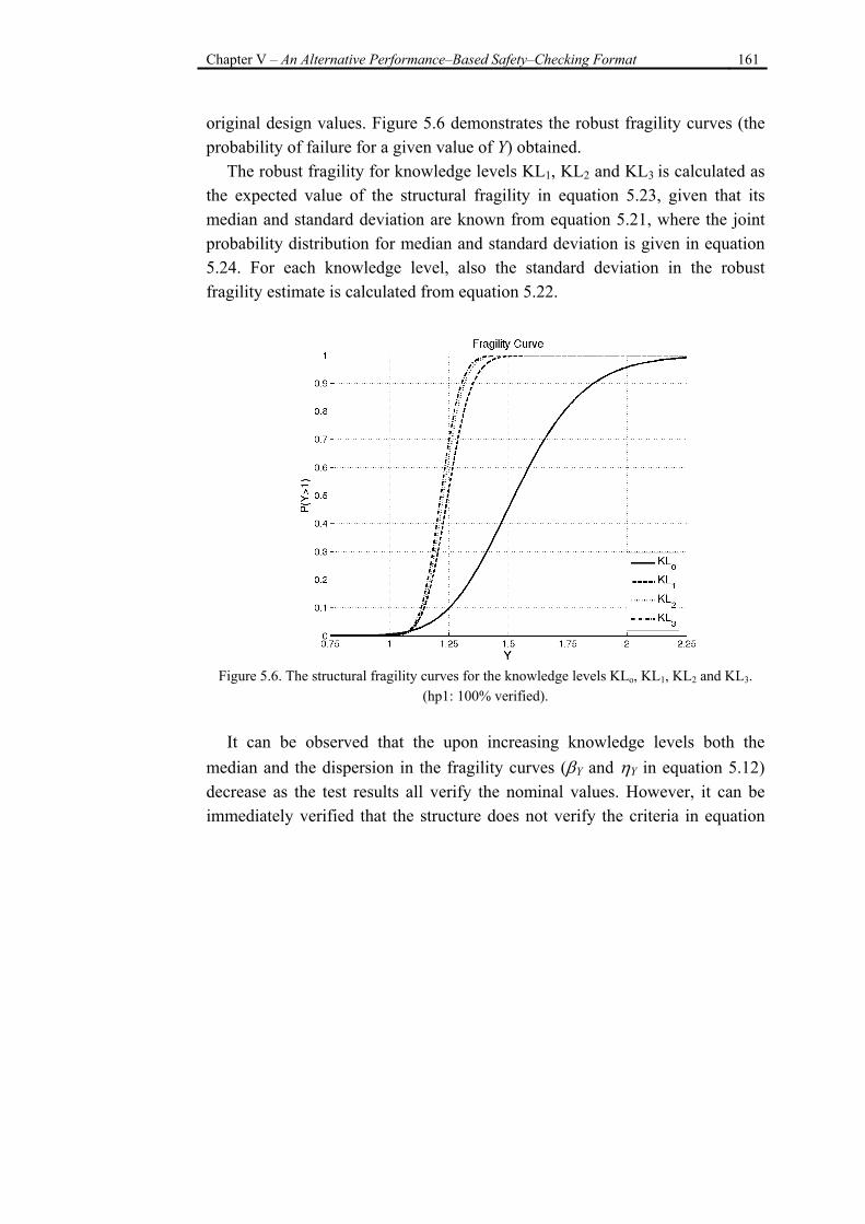
Chapter V – An Alternative Performance–Based Safety–Checking Format 161
original design values. Figure 5.6 demonstrates the robust fragility curves (the probability of failure for a given value of Y) obtained.
The robust fragility for knowledge levels KL1, KL2 and KL3 is calculated as the expected value of the structural fragility in equation 5.23, given that its median and standard deviation are known from equation 5.21, where the joint probability distribution for median and standard deviation is given in equation 5.24. For each knowledge level, also the standard deviation in the robust fragility estimate is calculated from equation 5.22.
Figure 5.6. The structural fragility curves for the knowledge levels KLo, KL1, KL2 and KL3.
(hp1: 100% verified).
It can be observed that the upon increasing knowledge levels both the median and the dispersion in the fragility curves (βY and ηY in equation 5.12) decrease as the test results all verify the nominal values. However, it can be immediately verified that the structure does not verify the criteria in equation
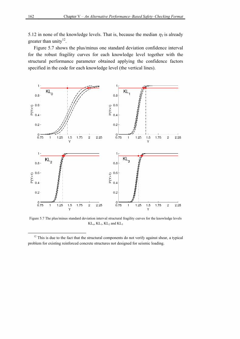
162 Chapter V – An Alternative Performance–Based Safety–Checking Format
5.12 in none of the knowledge levels. That is, because the median ηY is already greater than unity12.
Figure 5.7 shows the plus/minus one standard deviation confidence interval for the robust fragility curves for each knowledge level together with the structural performance parameter obtained applying the confidence factors specified in the code for each knowledge level (the vertical lines).
Figure 5.7 The plus/minus standard deviation interval structural fragility curves for the knowledge levels
KLo, KL1, KL2 and KL3
12 This is due to the fact that the structural components do not verify against shear, a typical
problem for existing reinforced concrete structures not designed for seismic loading.
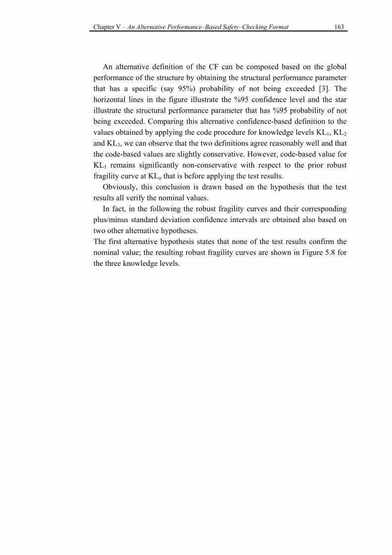
Chapter V – An Alternative Performance–Based Safety–Checking Format 163
An alternative definition of the CF can be composed based on the global
performance of the structure by obtaining the structural performance parameter that has a specific (say 95%) probability of not being exceeded [3]. The horizontal lines in the figure illustrate the %95 confidence level and the star illustrate the structural performance parameter that has %95 probability of not being exceeded. Comparing this alternative confidence-based definition to the values obtained by applying the code procedure for knowledge levels KL1, KL2 and KL3, we can observe that the two definitions agree reasonably well and that the code-based values are slightly conservative. However, code-based value for KL1 remains significantly non-conservative with respect to the prior robust fragility curve at KLo that is before applying the test results.
Obviously, this conclusion is drawn based on the hypothesis that the test results all verify the nominal values.
In fact, in the following the robust fragility curves and their corresponding plus/minus standard deviation confidence intervals are obtained also based on two other alternative hypotheses. The first alternative hypothesis states that none of the test results confirm the nominal value; the resulting robust fragility curves are shown in Figure 5.8 for the three knowledge levels.
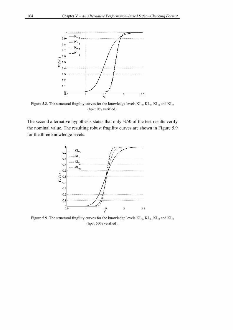
164 Chapter V – An Alternative Performance–Based Safety–Checking Format
Figure 5.8. The structural fragility curves for the knowledge levels KLo, KL1, KL2 and KL3
(hp2: 0% verified). The second alternative hypothesis states that only %50 of the test results verify the nominal value. The resulting robust fragility curves are shown in Figure 5.9 for the three knowledge levels.
Figure 5.9. The structural fragility curves for the knowledge levels KLo, KL1, KL2 and KL3
(hp3: 50% verified).
Chapter V – An Alternative Performance–Based Safety–Checking Format 165
Comparing figures 5.6, 5.8 and 5.9 it can be observed that the standard deviation of the fragility curves corresponding to each knowledge level remains invariant with respect to the test results while the median value significantly changes.
It should be mentioned that these are simplified hypotheses regarding the outcome of the tests assuming that the percentage of not verifying the test results is constant throughout all types of defects in the structure. 4.1.2. Verification of results using the standard Monte Carlo simulation
The results shown in the previous section are verified by reiterating the reliability assessments for the knowledge levels using the standard Monte Carlo simulation. For the prior knowledge level KL0, 500 realizations of the vector of uncertain parameters are simulated based on the prior probability distribution before implementing the test results. For knowledge levels KL1,Kl2 and KL3, given the reduced dispersion in the corresponding updated probability distributions, 200 simulation realizations are performed at each level.
Figure 5.10 illustrate how the fragility curves calculated based on MCS compare with the plus/minus one standard deviation interval provided by employing the efficient method described in chapter IV.
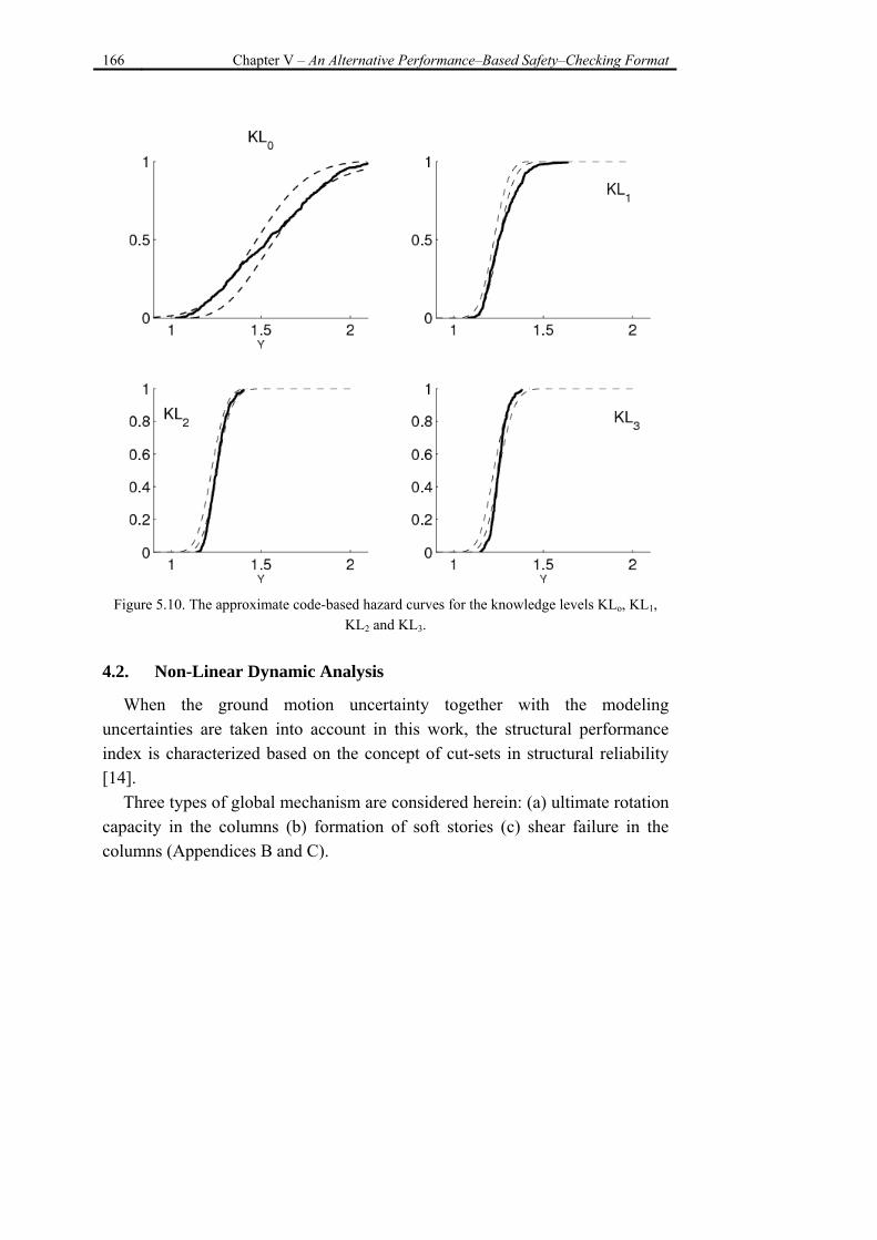
166 Chapter V – An Alternative Performance–Based Safety–Checking Format
Figure 5.10. The approximate code-based hazard curves for the knowledge levels KLo, KL1,
KL2 and KL3. 4.2. Non-Linear Dynamic Analysis
When the ground motion uncertainty together with the modeling uncertainties are taken into account in this work, the structural performance index is characterized based on the concept of cut-sets in structural reliability [14].
Three types of global mechanism are considered herein: (a) ultimate rotation capacity in the columns (b) formation of soft stories (c) shear failure in the columns (Appendices B and C).
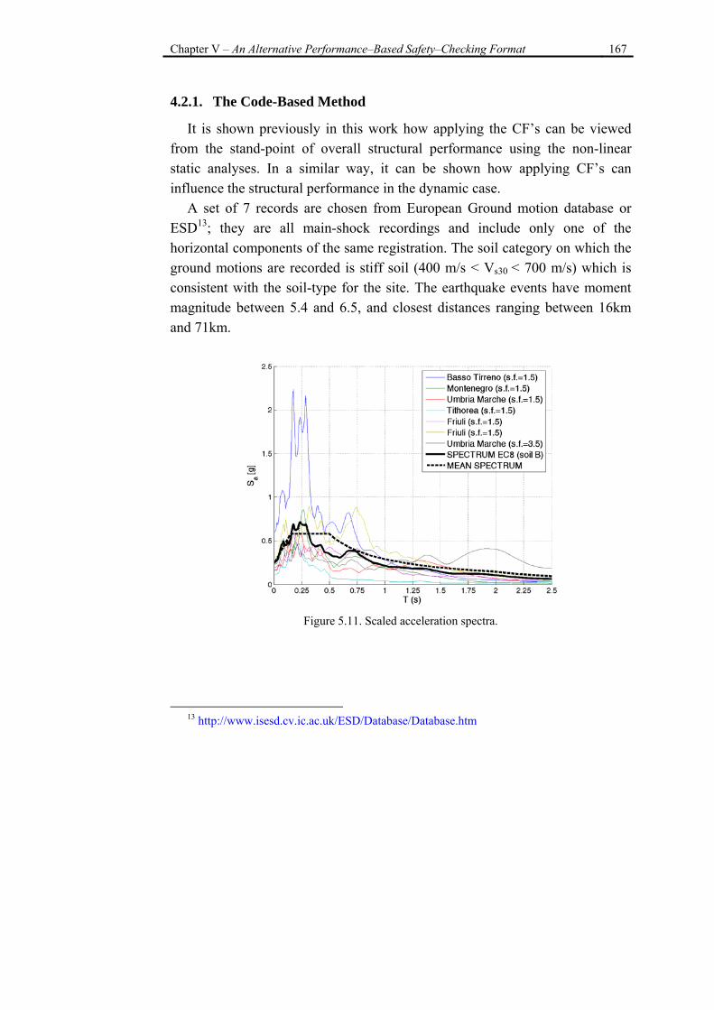
Chapter V – An Alternative Performance–Based Safety–Checking Format 167
4.2.1. The Code-Based Method
It is shown previously in this work how applying the CF’s can be viewed from the stand-point of overall structural performance using the non-linear static analyses. In a similar way, it can be shown how applying CF’s can influence the structural performance in the dynamic case.
A set of 7 records are chosen from European Ground motion database or ESD13; they are all main-shock recordings and include only one of the horizontal components of the same registration. The soil category on which the ground motions are recorded is stiff soil (400 m/s < Vs30 < 700 m/s) which is consistent with the soil-type for the site. The earthquake events have moment magnitude between 5.4 and 6.5, and closest distances ranging between 16km and 71km.
Figure 5.11. Scaled acceleration spectra.
13 http://www.isesd.cv.ic.ac.uk/ESD/Database/Database.htm
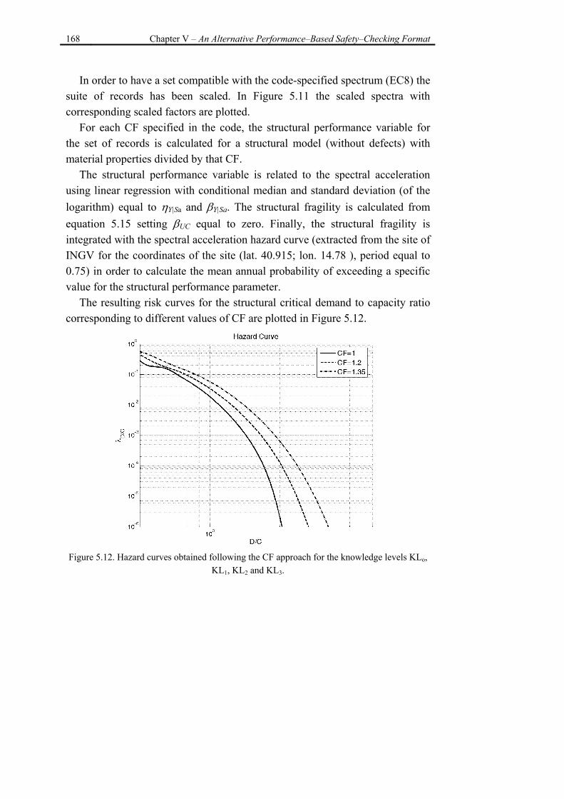
168 Chapter V – An Alternative Performance–Based Safety–Checking Format
In order to have a set compatible with the code-specified spectrum (EC8) the suite of records has been scaled. In Figure 5.11 the scaled spectra with corresponding scaled factors are plotted.
For each CF specified in the code, the structural performance variable for the set of records is calculated for a structural model (without defects) with material properties divided by that CF.
The structural performance variable is related to the spectral acceleration using linear regression with conditional median and standard deviation (of the logarithm) equal to ηY|Sa and βY|Sa. The structural fragility is calculated from equation 5.15 setting βUC equal to zero. Finally, the structural fragility is integrated with the spectral acceleration hazard curve (extracted from the site of INGV for the coordinates of the site (lat. 40.915; lon. 14.78 ), period equal to 0.75) in order to calculate the mean annual probability of exceeding a specific value for the structural performance parameter.
The resulting risk curves for the structural critical demand to capacity ratio corresponding to different values of CF are plotted in Figure 5.12.
Figure 5.12. Hazard curves obtained following the CF approach for the knowledge levels KLo,
KL1, KL2 and KL3.
Chapter V – An Alternative Performance–Based Safety–Checking Format 169
It should be noted that dispersion in these hazard curves reflects only the record-to-record variability. 4.2.2. Calculation of the Structural Reliability
The structural hazard curve for increasing levels of knowledge is calculated in this stage by integrating the robust fragilities and the spectral acceleration hazard curve at the site of the structure.
For each level of knowledge, the robust fragility is calculated from equations 5.21, 5.25, 5.26 and 5.27 using a set of 30 MC realizations of the structural model. At each knowledge level the robust hazard curve (i.e., the mean annual rate of exceeding the structural performance parameter) is calculated as the expected value of the hazard curve given that the median and the standard deviation for the structural fragility curve calculated from equation 5.25 are known. The median value for the fragility curve is estimated by employing the linear least squares as a function of the spectral acceleration at the fundamental mode of the structure. The joint probability distribution for the linear least squares coefficients is calculated from equation 5.27 and the probability distribution for the standard deviation of the fragility curve is calculated from equation 5.26 based on the results of a small set of 30 Monte Carlo simulations. The standard deviation as it can be seen in equation 5.25 can be calculated as the square root of the sum of squares of two parts representing the effect of ground motion uncertainty denoted by | aY Sβ and the structural modelling
uncertainty denoted by UCβ .
The set of MC realizations for each KL are generated based on the corresponding (updated) probability distributions. The suite of 30 records are the same adopted in chapter IV.
The resulting hazard curves are plotted in solid lines in Figure 5.13 knowledge levels KLo, KL1, KL2 and KL3. For each knowledge level, the hazard curve obtained by following the code procedure and applying the corresponding confidence factors is plotted in dashed lines. The horizontal line
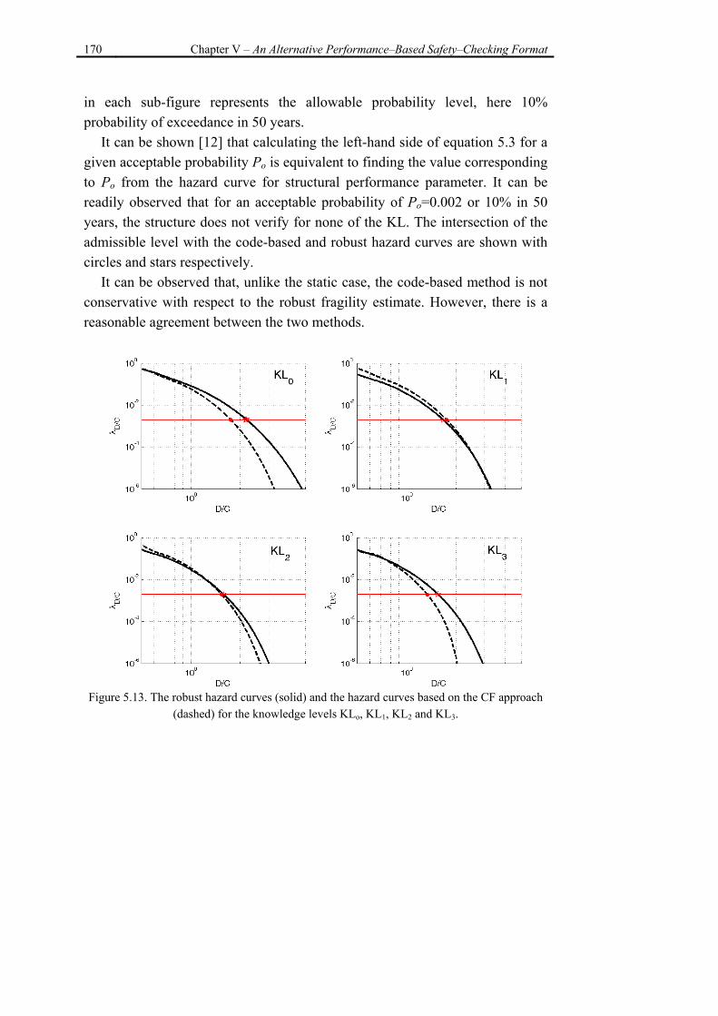
170 Chapter V – An Alternative Performance–Based Safety–Checking Format
in each sub-figure represents the allowable probability level, here 10% probability of exceedance in 50 years.
It can be shown [12] that calculating the left-hand side of equation 5.3 for a given acceptable probability Po is equivalent to finding the value corresponding to Po from the hazard curve for structural performance parameter. It can be readily observed that for an acceptable probability of Po=0.002 or 10% in 50 years, the structure does not verify for none of the KL. The intersection of the admissible level with the code-based and robust hazard curves are shown with circles and stars respectively.
It can be observed that, unlike the static case, the code-based method is not conservative with respect to the robust fragility estimate. However, there is a reasonable agreement between the two methods.
Figure 5.13. The robust hazard curves (solid) and the hazard curves based on the CF approach
(dashed) for the knowledge levels KLo, KL1, KL2 and KL3.

Chapter V – An Alternative Performance–Based Safety–Checking Format 171
5. Code-Based Implementation of the Alternative Performance-Based
Safety-Checking Format
Having calculated the structural reliability for different knowledge levels taking into account the structural modelling uncertainties, now the questions remains as to how such calculation can affect the code-based procedures. That is, how to formulate code-based performance-based assessments considering different sources of uncertainty. This section proposes a performance-based safety-checking format that accounts in an approximate way for both the amount and the outcome of in-site tests.
In the case of static analyses, the SAC-FEMA [6,7] formulation in equation 5.13 to obtain the x percentile of the structural performance parameter can be re-written as following:
1)(1
≤⋅γ⋅ βΦ−YxeY
) Eq. 5.28
where γ is a bias factor and βY is the standard deviation of the robust fragility curve. Y
)represents the structural performance parameter calculated based on
the median material properties based on the test results and nominal values for the structural detailing parameters. The bias factor γ (usually larger-than-unity) represent the factor that once multiplied by the nominal value Y
) leads to the
median value ηY. Tables 5.4 and 5.6 outline the parameters βY and γ values for the three
knowledge levels considered for the case study structure and based on static analyses. The three columns represent the three simplified hypotheses adopted previously regarding the outcome of the test results.
Table 5.7 outline these parameters for the knowledge level KLo before the tests are preformed.
It can be observed that based on the prior distributions considered herein, considering the structural modeling uncertainties can affect the structural reliability up to %15. Considering the hypothesis that %100 of the test results
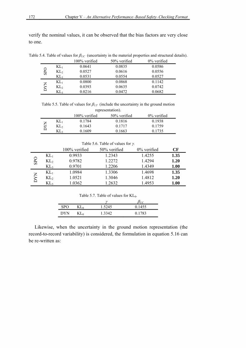
172 Chapter V – An Alternative Performance–Based Safety–Checking Format
verify the nominal values, it can be observed that the bias factors are very close to one. Table 5.4. Table of values for βUC (uncertainty in the material properties and structural details).
100% verified 50% verified 0% verified
SPO
KL1 0.0641 0.0835 0.0586 KL2 0.0527 0.0616 0.0556 KL3 0.0531 0.0554 0.0527
DY
N KL1 0.0800 0.0868 0.1142
KL2 0.0393 0.0635 0.0742 KL3 0.0216 0.0472 0.0682
Table 5.5. Table of values for βUT (include the uncertainty in the ground motion
representation). 100% verified 50% verified 0% verified
DY
N KL1 0.1784 0.1816 0.1938
KL2 0.1643 0.1717 0.1759 KL3 0.1609 0.1663 0.1735
Table 5.6. Table of values for γ.
100% verified 50% verified 0% verified CF
SPO
KL1 0.9933 1.2343 1.4255 1.35 KL2 0.9782 1.2272 1.4294 1.20 KL3 0.9701 1.2206 1.4349 1.00
DY
N KL1 1.0984 1.3306 1.4698 1.35
KL2 1.0521 1.3046 1.4812 1.20 KL3 1.0362 1.2632 1.4953 1.00
Table 5.7. Table of values for KL0.
γ βUC SPO KL0 1.5245 0.1455 DYN KL0 1.3342 0.1783
Likewise, when the uncertainty in the ground motion representation (the
record-to-record variability) is considered, the formulation in equation 5.16 can be re-written as:
Chapter V – An Alternative Performance–Based Safety–Checking Format 173
22|
12| )(2
1UCaSYaSY xb
k
eeY β+βΦβ −
≤⋅γ⋅)
Eq. 5.29
where γ is a bias factor and βUC represent the over-all effect of structural modeling uncertainties. Y
) represents the structural performance parameter
calculated based on the median material properties obtained from the test results and nominal values for the structural detailing parameters. Y)
is calculated by performing linear least squares as a function of the first-mode spectral acceleration based on the set of 7 records. The bias factor γ (usually larger-than-unity) is a factor that once multiplied by the nominal value Y)
leads to the median value for the structural performance parameter calculated using the maximum likelihood estimates for the regression coefficients obtained from the probability distribution in equation 5.27. Table 5.4 and 5.6 tabulate the γ and βUC for different knowledge levels and test outcomes based on non-linear time-history analyses. The same coefficients for the KL0 knowledge level are listed separately in Table 5.7.
The tables reported in this section are classified based on the type of analysis, level of knowledge and the outcome of the test results. These tables, once calculated for representative classes of structures and periods of construction, can be employed, in lieu of more thorough probability-based methods, for performance-based assessment of existing buildings.
It should be noted that comparing the results shown in Table 5.4 and Table 5.5, there is a significant increase in the value of the dispersion of the structural fragility considering also the uncertainty in the ground motion representation. This emphasizes the importance of considering the uncertainties in the representation of the ground motion in the code-based procedure. 6. Conclusions
Quantifying the uncertainty in the structural modeling parameters related to the level of knowledge about an existing structure is one of the main challenges in seismic performance assessment of existing buildings. The discrete
174 Chapter V – An Alternative Performance–Based Safety–Checking Format
knowledge levels (KL) defined by the code leave significant room for interpretation. In other words, the code-based definition for KL does not lead to a unique configuration of tests and inspections. Moreover, it is not clear which level of structural reliability does the application of the confidence factors guarantee. Hence, with the emerging of performance-based design and life-cycle cost analysis in earthquake engineering, there seems to be a need for a code-based method that bridges the different knowledge levels to structural reliability and probabilistic structural performance assessment.
Intuitively speaking, the relation between the confidence factors and the knowledge levels seems to be highly dependent on the results of in-situ tests and inspections. Therefore, it is necessary to adopt a general probabilistic framework for updating the probability distribution for the uncertain parameters based on the test results. The Bayesian framework for inference seems to be perfectly suitable for this end; as it can sequentially incorporate the incoming tests and inspection results without discarding any prior information available.
The uncertain parameters considered include the material properties, the construction detailing parameters and, in the case of the dynamic analyses, the uncertainty in the ground motion representation. For each knowledge level, the probability distributions for the uncertain parameters are updated using the Bayesian updating frame work.
In the absence of test results abiding exactly with the code prescriptions, an idealized situation is considered in which all of the test results verify the original design values. Obviously, the methodology presented is general with respect to the outcome of the test and inspections.
The uncertain parameters are divided in groups (emulating various homogenous construction zones). It is assumed that the uncertain parameters belonging to distinct groups are fully un-correlated and only the uncertain parameters inside a given group can be correlated. It should be noted that decisions on possible groupings of the uncertain parameters can affect significantly the global performance assessment of the structure.
Chapter V – An Alternative Performance–Based Safety–Checking Format 175
It is observed that for increasing knowledge levels, the estimates for the structural performance tend to get very close. This is while the structural performance parameters corresponding to the confidence factors tend to remain fairly distinct.
The approximate code-based method manages to provide reasonable estimates of the structural performance. However, it is not guaranteed that it would remain conservative with respect to the probability-based estimates as is the case of the assessments performed using the non-linear time-history analyses.
As a final note particular to the case-study considered, it should be mentioned that the critical value for the structural performance variable is almost always governed by the shear failure in structural components. This is a typical problem for the existing reinforced concrete structures designed only for the gravity loads.
In the context of a code-based performance-based assessment approach, different classes of existing buildings can be identified and analyzed. The prior probability distributions for the structural modeling uncertainties can be classified and tabulated based on the surveys of expert opinion and experience. It is important to identify those uncertain parameters that affect the structural response in a dominant way (e.g., the material properties, the stirrup spacing). These prior probability distributions are going to be updated based on the results of tests and inspections. The updated probability distributions are constructed for various KL’s, based on special cases of tests and inspection results.
Finally, for different classes of structures and different levels of knowledge (and a few special cases of inspection results), the best-estimate values for the parameters defining the adopted safety-checking format and/or structural fragility can be tabulated.
It should be addressed that when tackling the problem of performance assessment of existing buildings, it is important to lay out a range of methods. In this manner, the suitable method can be selected as a function of the importance of the structure and the level of precision desired. For instance, in

176 Chapter V – An Alternative Performance–Based Safety–Checking Format
the case of strategic buildings, it would be useful to recommend some relatively simple and approachable methods suitable for case-specific estimation of the parameters defining the safety checking format and/or structural fragility.

Chapter V – An Alternative Performance–Based Safety–Checking Format 177
7. References
[1] Franchin P., Pinto P. E., Pathmanathan R., Assessing the adequacy of a single confidence factor in accounting for epistemic uncertainty, Convegno RELUIS “Valutazione e riduzione della vulnerabilità sismica di edifici esistenti in cemento armato”, Roma 29-30 maggio 2008.
[2] AISC. Manual of Steel Construction Load and Resistannce Factor Design. Second Edition, American Institute of Steel Construction Inc., Chigaco, IL, 1994.
[3] Jalayer F., Iervolino I., Manfredi G., “Structural modeling uncertainties and their influence on seismic assessment of existing RC structures”, submitted to Structural Safety, 2008.
[4] Department of Energy (DOE), 1994. Natural Phenomena Hazards Design and Evaluation Criteria for Department of Energy Facilities, DOE-STD-1020-94, U.S. Department of Energy, Washington, D.C.
[5] Federal Emergency Management Agency (FEMA), 2000. Recommended Seismic Design Criteria for New Steel Moment-Frame Buildings, FEMA-350, SAC Joint Venture, Washington, D.C.
[6] Federal Emergency Management Agency (FEMA), 2000. Recommended Seismic Evaluation and Upgrade Criteria for Existing Welded Steel Moment-Frame Buildings, FEMA-351, SAC Joint Venture, Washington, D.C.
[7] Federal Emergency Management Agency (FEMA), 2000. Recommended Post-Earthquake Evaluation and Repair Criteria for Welded Steel Moment-Frame Buildings, FEMA-352, SAC Joint Venture, Washington, D.C.
[8] Federal Emergency Management Agency (FEMA), 2000. Pre-Standard and Commentary for the Seismic Rehabilitation of Buildings. FEMA 356, Washington, D.C.
[9] CEN, European Committee for Standardisation TC250/SC8/ [2003] “Eurocode 8: Design Provisions for Earthquake Resistance of Structures, Part 1.1: General rules, seismic actions and rules for buildings,” PrEN1998-1.
[10] Cornell, C. A., Jalayer, F., Hamburger, R. O., and Foutch, D. A., (2002), The probabilistic basis for the 2000 SAC/FEMA steel moment frame guidelines, ASCE Journal of Structural Engineering, Vol. 128, No.4, pp. 526-533.
178 Chapter V – An Alternative Performance–Based Safety–Checking Format
[11] Jalayer F, Franchin P, Pinto PE. A scalar damage measure for seismic reliability analysis of RC frames. Earthquake Engineering and Structural Dynamics. 36:2059-2079, 2007.
[12] Jalayer, F., Cornell, C. A. (2008), “Alternative Nonlinear Demand Estimation Methods for Probability-Based Seismic Assessments”, Early View Earthquake Engineering and Structural Dynamics, 2008.
[13] Fajfar, P. Capacity spectrum method based on inelastic demand spectra, Earthquake Engineering and Structural Dynamics; 28:979–93, 1999.
[14] Ditlevsen O, Masden H. Structural Reliability Methods, June 1996; John Wiley & Sons Inc.
[15] Verderame, G.M., Manfredi, G., Frunzio G., Le proprietà meccaniche dei calcestruzzi impiegati nelle strutture in cemento armato realizzate negli anni ’60, X Congresso Nazionale “L’ingegneria Sismica in Italia”, Potenza-Matera 9-13 settembre 2001a.
[16] Verderame, G.M., Stella, A., Cosenza, E., Le proprietà meccaniche degli acciai impiegati nelle strutture in cemento armato realizzate negli anni ’60, X Convegno Nazionale “L'Ingegneria Sismica in Italia”, Potenza e Matera 9-13 Settembre 2001b.
[17] Jalayer F., L. Elefante, Iervolino I., Manfredi G., “Small-Sample Bayesian Inference for Estimation of Structural Modeling Uncertainty Parameters in Seismic Assessment of Existing RC Buildings”, ICOSSAR09 Conference, 2009.
[18] Box, G.E.P. and Tiao, G.C., Bayesian Inference in Statistical Analysis, Wiley Interscience, 1992.
[19] Ordinanza del Presidente del Consiglio dei Ministri (OPCM) n. 3431, Ulteriori modifiche ed integrazioni all'ordinanza del Presidente del Consiglio dei Ministri n. 3274 del 20 marzo 2003. Gazzetta Ufficiale della Repubblica Italiana n. 107 del 10-5-2005 (Suppl. Ordinario n.85), 2005.
[20] CS..LL.PP, DM 14 gennaio, Norme Techniche per le Costruzioni. Gazzetta Ufficiale della Repubblica Italiana, 29, 2008a (in Italian).
[21] CS.LL.PP, DM 14 gennaio, Istruzioni per l'applicazione delle Norme Techniche delle costruzioni. Ministero della Infrastruttura, 29, 2008b (in Italian).

Chapter VI – How to Characterize Prior Probability Distribution for Structural Details: a Survey for Professional Engineers 179
Chapter VI
How to Characterize Prior Probability Distribution for Structural Details: a Survey for Professional Engineers
1. Introduction
Developing prior distributions is undoubtedly the most controversial aspect of any Bayesian analysis [1,2]. Considerable care should be taken when selecting priors and the process by which priors are selected must be documented carefully. This is because inappropriate choices for priors can lead to incorrect inferences.
There are two types of priors: informative and non-informative (or "reference") [3] define a non-informative prior as one that provides little information relative to the analyzed experiment. Informative prior distributions, on the other hand, summarise the evidence about the parameters concerned from many sources and often have a considerable impact on the results.
Using informative prior distributions allows the incorporation of information available to analysts from the literature and in light of their experience. However, using informative priors is not a trivial task because their subjective nature.
180 Chapter VI – How to Characterize Prior Probability Distribution for Structural Details:
a Survey for Professional Engineers
Uniform priors are generally chosen when non-informative priors are needed, as it has been used in chapter V for structural details. However, given the versatility of the Bayesian updating framework in incorporating prior information, it is important to characterize prior probability distributions for construction details based on qualitative and collective information coming from experts in the field.
In relation to the probability distributions related to construction details, a survey for professional engineers has been prepared in order to be able to characterize these prior distributions in relation to expert opinion; the survey is presented in this chapter together with the preliminary results obtained by interviewing a small sample of professionals in order to test it. 2. The Survey for Professional Engineers
In the framework of the alternative performance-based safety-checking format proposed in the previous chapter, the prior probability distributions for the structural modeling uncertainties can be classified and tabulated based on various surveys of expert opinion and experience.
One of the main characteristics of the construction details is that possible deviations from the original configurations are mostly taken into account in those cases leading to undesirable effects. This justifies why the uncertainties related to construction details are usually referred to as the structural defects.
In this section the steps followed for the development of the survey for professional engineers relative to the uncertainty in structural details are briefly summarized.
• First of all it is necessary to identify those modeling uncertainties that affect the structural response in a dominant way. Obviously these choices is always related to the level of sophistication that is adopted for the finite element model of the structure under assessment.
• Once a source of uncertainty related to structural details is identified it is necessary to determinate a quantifiable parameter or variable that is representative for the identified source of uncertainty.

Chapter VI – How to Characterize Prior Probability Distribution for Structural Details: a Survey for Professional Engineers 181
• Then, it is necessary to assign a reasonable interval of values that the identified quantifiable parameter can assume. In this phase, the professional engineer can also indicate the most plausible value of the quantifiable parameter, in relation of her/his experience, in the assigned interval.
• Moreover for each source of uncertainty identified and its corresponding quantifiable parameter it is necessary to investigate its systematic nature. This serves in identifying the zone in which the parameter is going to be modelled as constant.
The compiling of the survey is anonymous, but two questions are included in order to have some information about the engineer’s professional experience. First, the engineer has to state the professional association he belongs to, in order to consider the engineering practice typical of the reference province in which he operates. Name (facultative field) Surname (facultative field) Affiliation (facultative field) Professional Association (required field)
Furthermore a question related to the number of RC structures that the professional has designed, super-visioned and/or evaluated before and after 1976, is included. RC buildings constructed before 1976
# designed or super-visioned # evaluated or assessed
RC buildings constructed after 1976
# designed or super-visioned # evaluated or assessed
This additional information can be used in order to weight the results of each compiled survey in relation to the experience of the engineer.
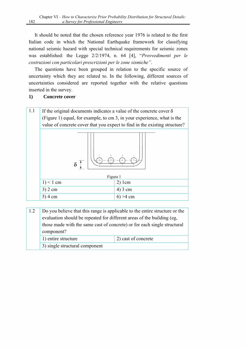
182 Chapter VI – How to Characterize Prior Probability Distribution for Structural Details:
a Survey for Professional Engineers
It should be noted that the chosen reference year 1976 is related to the first Italian code in which the National Earthquake framework for classifying national seismic hazard with special technical requirements for seismic zones was established: the Legge 2/2/1974, n. 64 [4], “Provvedimenti per le costruzioni con particolari prescrizioni per le zone sismiche”.
The questions have been grouped in relation to the specific source of uncertainty which they are related to. In the following, different sources of uncertainties considered are reported together with the relative questions inserted in the survey. 1) Concrete cover 1.1 If the original documents indicates a value of the concrete cover δ
(Figure 1) equal, for example, to cm 3, in your experience, what is the value of concrete cover that you expect to find in the existing structure?
Figura 1
1) < 1 cm 2) 1cm 3) 2 cm 4) 3 cm 5) 4 cm 6) >4 cm
1.2 Do you believe that this range is applicable to the entire structure or the
evaluation should be repeated for different areas of the building (eg, those made with the same cast of concrete) or for each single structural component? 1) entire structure 2) cast of concrete 3) single structural component

Chapter VI – How to Characterize Prior Probability Distribution for Structural Details: a Survey for Professional Engineers 183
2) Bars anchorage 2.1 In the original documents it is indicated that the anchor to be used is a
hook. Among 100 hooks, in your experience, how many of them are well done in the existing structure? That is, how many of them are closed with an angle larger then 150 ° (Figure 2, A) ?
Figura 2
1) 100 3) 50 5) 10 2) 80 4) 20 6) 0 Among the hooks that are not properly closed, how many are closed with an angle between 90 ° and150° (Figure 2, B)? 1) 100 3) 50 5) 10 2) 80 4) 20 6) 0
2.2 Do you believe that the previous answer is relative to the entire
structure, to a single cast of concrete or to each single structural component? 1) entire structure 2) cast of concrete 3) single structural component
2.3 In the original documents an anchoring length of cm 25 is shown. In your experience, what is the value of the anchoring length you expect to find in the existing structure? 1) 10 cm 3) 15 cm 2) 20 cm 4) 25 cm
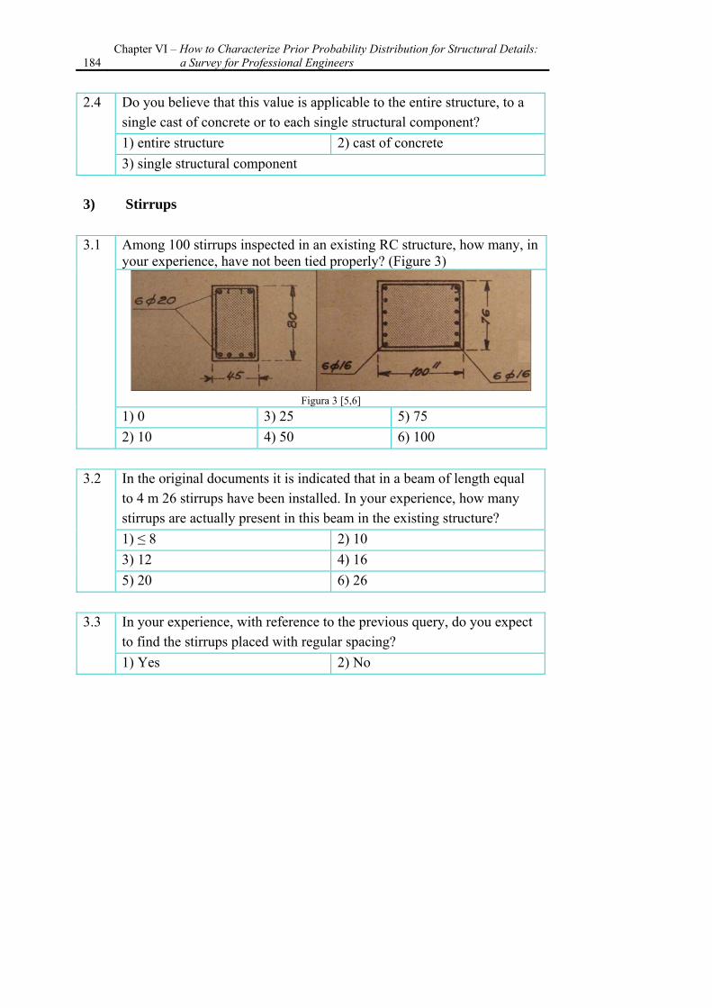
184 Chapter VI – How to Characterize Prior Probability Distribution for Structural Details:
a Survey for Professional Engineers
2.4 Do you believe that this value is applicable to the entire structure, to a single cast of concrete or to each single structural component? 1) entire structure 2) cast of concrete 3) single structural component
3) Stirrups 3.1 Among 100 stirrups inspected in an existing RC structure, how many, in
your experience, have not been tied properly? (Figure 3)
Figura 3 [5,6]
1) 0 3) 25 5) 75 2) 10 4) 50 6) 100
3.2 In the original documents it is indicated that in a beam of length equal
to 4 m 26 stirrups have been installed. In your experience, how many stirrups are actually present in this beam in the existing structure? 1) ≤ 8 2) 10 3) 12 4) 16 5) 20 6) 26
3.3 In your experience, with reference to the previous query, do you expect
to find the stirrups placed with regular spacing? 1) Yes 2) No

Chapter VI – How to Characterize Prior Probability Distribution for Structural Details: a Survey for Professional Engineers 185
3.4 The original documents indicate that in a beam of length equal to 4 m 26 stirrups have been installed. How many stirrups do you expect to find in cm 50 of the beam near the supports? 1) 2 2) 3 3) 4 4) 6 and how many in a meter of beam span? 1) 2 2) 3 3) 4 4) 6
3.5 Do you believe that this value is applicable to the entire structure, to a
single cast of concrete or to each single structural component? 1) entire structure 2) cast of concrete 3) single structural component
3.6 Among 10 beam-column joints of the existing structure, in your
experience, how often the stirrup in the beam-column connection may be absent? 1) ≤ 2 2) 4 3) 6 4) 8 5) 10
3.7 In the case of absence of stirrup in the beam-column connection, how
far away from the connection do you believe to find the first stirrup? 1) 2 cm 2) 5 cm 3) 10 cm 4) 20 cm
3.8 The original documents indicate that in a meter of a 3 m long column
20 stirrups have been installed. In your experience, how many stirrups are actually present in a meter of column in the existing structure? 1) 6 2) 10 3) 16 4) 20

186 Chapter VI – How to Characterize Prior Probability Distribution for Structural Details:
a Survey for Professional Engineers
3.9 In your experience, with reference to the previous question, do you
expect to find the stirrups placed with regular space? 1) Yes 2) No
3.10 The original documents indicate that in a 3 m long column 20 stirrups
have been installed. How many stirrups do you believe to find in 50 cm of the column corresponding to the lower end? 1) 2 2) 3 3) 4 4) 5 5) 6 6) ≥ 7
3.11 Do you believe that this value is applicable to the entire structure, to a
single cast of concrete or to each single structural component? 1) entire structure 2) cast of concrete 3) single structural component
Chapter VI – How to Characterize Prior Probability Distribution for Structural Details: a Survey for Professional Engineers 187
4) Reinforcing bars 4.1 The original documents indicate that in order to reinforce a specified
storey in the structure two different types of reinforcement diameters φA and φB, with φA <φB (e.g., φ12 and φ14) have been used. Do you believe it is possible that in a beam reinforced with straight longitudinal bars of diameter φA and φB, the two diameters have been confused? 1) Yes 2) No Do you believe it is possible that in a beam reinforced with straight longitudinal bars of diameter φA and bent longitudinal bars of diameter φB, the two diameters have been inverted? 1) Yes 2) No Do you believe it is possible that in a column reinforced in a direction with bars of diameter φA and in the other direction with bars of diameter φB, reinforcement in the two directions have been reversed? 1) Yes 2) No
4.2 Assuming that the original documents indicate that in order to reinforce
a certain level of the structure 50 reinforcing bars of diameter φA and 50 of diameter φB have been used, with φA < φB. Which is the total number of reinforcing bars of diameter φA do you expect to find in the existing structure? 1) 35 φΑ 2) 45 φΑ 3) 55 φΑ 4) 65 φΑ 5) 75 φΑ 6) 85 φΑ
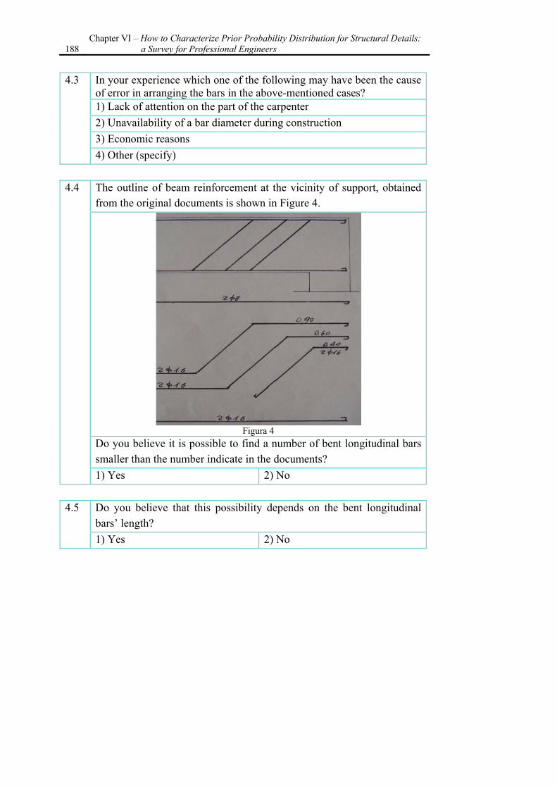
188 Chapter VI – How to Characterize Prior Probability Distribution for Structural Details:
a Survey for Professional Engineers
4.3 In your experience which one of the following may have been the cause of error in arranging the bars in the above-mentioned cases? 1) Lack of attention on the part of the carpenter 2) Unavailability of a bar diameter during construction 3) Economic reasons 4) Other (specify)
4.4 The outline of beam reinforcement at the vicinity of support, obtained
from the original documents is shown in Figure 4.
Figura 4
Do you believe it is possible to find a number of bent longitudinal bars smaller than the number indicate in the documents? 1) Yes 2) No
4.5 Do you believe that this possibility depends on the bent longitudinal
bars’ length? 1) Yes 2) No

Chapter VI – How to Characterize Prior Probability Distribution for Structural Details: a Survey for Professional Engineers 189
4.6 Among 10 beam sections whose reinforcement in the vicinity of support is specified Figure 4, in your experience, in how many of them one bent longitudinal bar would be missing with respect to what specified in the original documents? 1) 0 2) 1 3) 2 4) 5 5) 7 6) 10
4.7 Do you believe that it is possible that the missing shaped bars are more
than one? 1) Yes 2) No
190 Chapter VI – How to Characterize Prior Probability Distribution for Structural Details:
a Survey for Professional Engineers
5) Column superposition length 5.1 In your experience, do the original documents normally indicate the
overlapping length of the reinforcement of the columns between successive levels? 1) Yes 2) No
5.2 If the original documents indicate a superposition length of 100 cm for
an interstory height of 3 m, what is the value of the superposition length that you expect to find in the existing structure? 1) 10 cm 2) 25 cm 3) 50 cm 4) 60 cm 5) 75 cm 6) 100 cm
5.3 In your experience, if the original documents do not indicate the
superposition length for columns, for an interstory height of 3 m, what is the value of the superposition length that you expect to find in the existing structure? 1) 10 cm 2) 25 cm 3) 50 cm 4) 60 cm 5) 75 cm 6) 100 cm
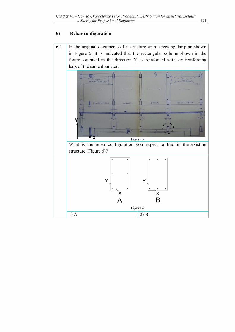
Chapter VI – How to Characterize Prior Probability Distribution for Structural Details: a Survey for Professional Engineers 191
6) Rebar configuration 6.1 In the original documents of a structure with a rectangular plan shown
in Figure 5, it is indicated that the rectangular column shown in the figure, oriented in the direction Y, is reinforced with six reinforcing bars of the same diameter.
Figura 5
What is the rebar configuration you expect to find in the existing structure (Figure 6)?
Figura 6
1) A 2) B
X
Y

192 Chapter VI – How to Characterize Prior Probability Distribution for Structural Details:
a Survey for Professional Engineers
7) Geometrical properties of structural elements 7.1 The original documents of a structure indicate that the cross section of a
beam with a length equal to 4 m is characterized by a width of 40 cm and a height of 60 cm. In your experience, what is the actual size of the base of the beam width in the existing structure? 1) ≤ 30 cm 2) 35 cm 3) 38 cm 4) 40 cm 5) 43 cm 6) ≥ 45 cm And what is the actual size of the beam height in the existing structure? 1) ≤ 50 cm 2) 55 cm 3) 58 cm 4) 60 cm 5) 63 cm 6) ≥ 65 cm
7.2 The original documents of a structure indicate that a column with a
height of 3 m, has a square cross section of 40 cmx40 cm. In your experience, what is the actual dimension of the side of the column section in the existing structure? 1) ≤ 30 cm 2) 35 cm 3) 38 cm 4) 40 cm 5) 43 cm 6) ≥ 45 cm
Moreover, in the survey few other questions have been included in order to
leave the opportunity to the professional engineers to suggest other type of structural defects that they may have encountered in their professional experience.

Chapter VI – How to Characterize Prior Probability Distribution for Structural Details: a Survey for Professional Engineers 193
8.1 Have you encountered in your professional experience, other types of "defects", not reported in this survey? 1) Yes 2) No If so, can you describe the "defect" type.
1) “defect” type
2) “defect” type
3) “defect” type
8.2 Can you indicate, for each type of described "defect", a range of values
that the parameter associated with the "defect" may assume? How often it is possible to find such a "defect" in 10 inspections directly operated on the existing structure.
1) Range Revealed in 10 inspections
2) Range Revealed in 10 inspections
3) Range Revealed in 10 inspections
8.3 Please indicate any additional comments in space provided below.
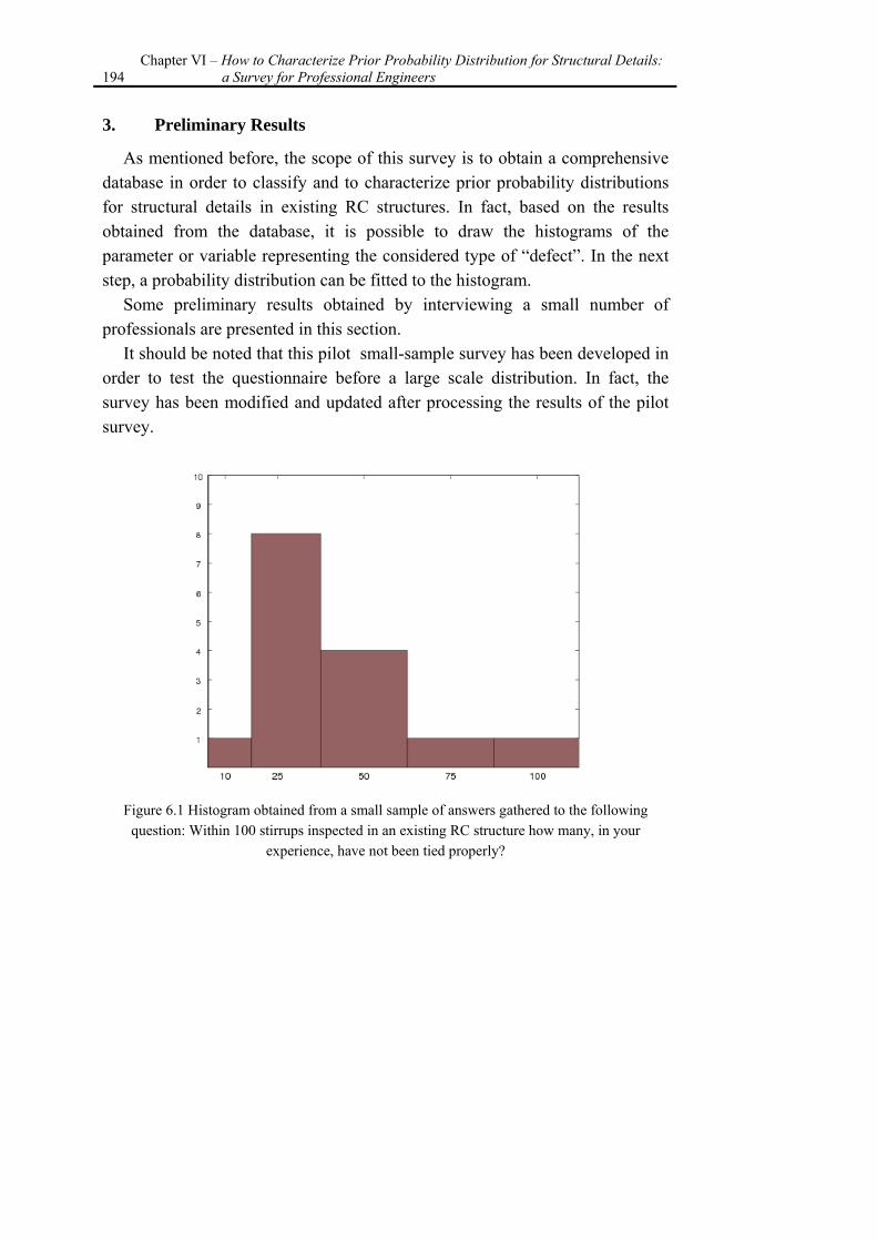
194 Chapter VI – How to Characterize Prior Probability Distribution for Structural Details:
a Survey for Professional Engineers
3. Preliminary Results
As mentioned before, the scope of this survey is to obtain a comprehensive database in order to classify and to characterize prior probability distributions for structural details in existing RC structures. In fact, based on the results obtained from the database, it is possible to draw the histograms of the parameter or variable representing the considered type of “defect”. In the next step, a probability distribution can be fitted to the histogram.
Some preliminary results obtained by interviewing a small number of professionals are presented in this section.
It should be noted that this pilot small-sample survey has been developed in order to test the questionnaire before a large scale distribution. In fact, the survey has been modified and updated after processing the results of the pilot survey.
Figure 6.1 Histogram obtained from a small sample of answers gathered to the following
question: Within 100 stirrups inspected in an existing RC structure how many, in your experience, have not been tied properly?
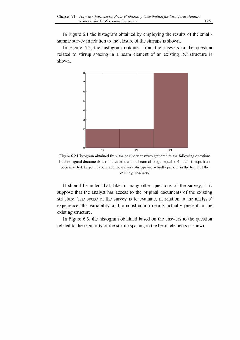
Chapter VI – How to Characterize Prior Probability Distribution for Structural Details: a Survey for Professional Engineers 195
In Figure 6.1 the histogram obtained by employing the results of the small-sample survey in relation to the closure of the stirrups is shown.
In Figure 6.2, the histogram obtained from the answers to the question related to stirrup spacing in a beam element of an existing RC structure is shown.
Figure 6.2 Histogram obtained from the engineer answers gathered to the following question: In the original documents it is indicated that in a beam of length equal to 4 m 24 stirrups have been inserted. In your experience, how many stirrups are actually present in the beam of the
existing structure?
It should be noted that, like in many other questions of the survey, it is suppose that the analyst has access to the original documents of the existing structure. The scope of the survey is to evaluate, in relation to the analysts’ experience, the variability of the construction details actually present in the existing structure.
In Figure 6.3, the histogram obtained based on the answers to the question related to the regularity of the stirrup spacing in the beam elements is shown.
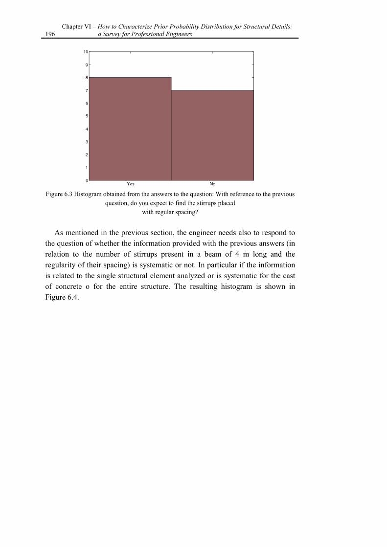
196 Chapter VI – How to Characterize Prior Probability Distribution for Structural Details:
a Survey for Professional Engineers
Figure 6.3 Histogram obtained from the answers to the question: With reference to the previous
question, do you expect to find the stirrups placed with regular spacing?
As mentioned in the previous section, the engineer needs also to respond to
the question of whether the information provided with the previous answers (in relation to the number of stirrups present in a beam of 4 m long and the regularity of their spacing) is systematic or not. In particular if the information is related to the single structural element analyzed or is systematic for the cast of concrete o for the entire structure. The resulting histogram is shown in Figure 6.4.
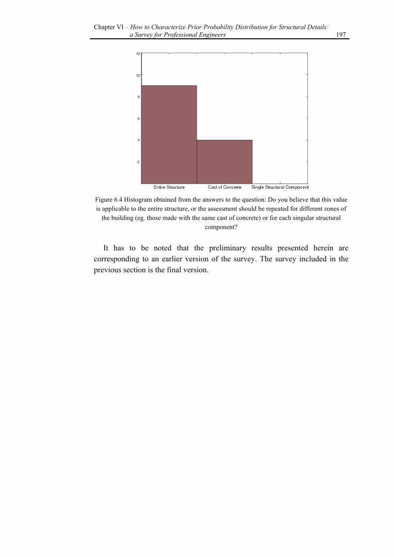
Chapter VI – How to Characterize Prior Probability Distribution for Structural Details: a Survey for Professional Engineers 197
Figure 6.4 Histogram obtained from the answers to the question: Do you believe that this value is applicable to the entire structure, or the assessment should be repeated for different zones of
the building (eg. those made with the same cast of concrete) or for each singular structural component?
It has to be noted that the preliminary results presented herein are
corresponding to an earlier version of the survey. The survey included in the previous section is the final version.

198 Chapter VI – How to Characterize Prior Probability Distribution for Structural Details:
a Survey for Professional Engineers
4. References
[1] Lindley, D.V. 1983. Theory and practice of Bayesian statistics. The Statistician 32, 1-11..
[2] Walters, C.[J.] and D. Ludwig. Calculation of Bayes posterior probability distributions for key population parameters. Can. J. Fish. Aquat. Sci. 51, 713-722.
[3] Box, G.E.P. and Tiao, G.C., Bayesian Inference in Statistical Analysis, Wiley Interscience, 1992.
[4] Legge 2 febbraio 1974 n. 64, “Provvedimenti per le costruzioni con particolari prescrizioni per le zone sismiche” (in Italian).
[5] Santarella L. “Il cemento armato – Le applicazioni alle costruzioni civili ed industriali”, Edizione Hoepli 1968.
[6] Pagano M. “Teoria degli edifici - Edifici in cemento armato”, Napoli, Edizione Liguori 1968.

Conclusions 199
Conclusions
This thesis focuses on the seismic assessment of existing RC buildings, with particular attention to the various sources of uncertainty that are involved in this problem.
A significant part of the total seismic risk in Italy, evaluated in economic terms, comes from the various type of damages endured by the existing buildings. This is the case for several other European countries in which the average service life for buildings is larger than that of countries like the United States. Therefore, management of existing building stock is a major concern in such regions.
As a result, more recent European seismic guidelines (EC8, OPCM, NTC) pay particular attention to seismic assessment of existing structures, which is distinguished from that of the new construction by lack of information about both the original features and the current state of building in consideration. Therefore, the assessment of existing RC structures is strongly affected by uncertainties in structural modeling, which may be comparable with those related to the representation of the ground motion.
Recent European codes seem to summarize the effect of these uncertainties in the so-called confidence factors that are applied to mean material properties, in order to allow for a certain level of conservatism when performing seismic assessment of an existing structure. This leads to using material strength values smaller then those determined based on available knowledge. The confidence factors are defined depending on the level of knowledge acquired for the
200 Conclusions
structure on the basis of specific test (destructive and non-destructive) and in-situ inspection results.
Although the confidence factors are applied to the properties of materials, the uncertainties in structural modeling are not limited to them and include also other structural detailing parameters (e.g., reinforcement detailing, cover thickness, etc.) entering into the seismic assessment problem. The variations in structural detailing parameters can prove quite significant to the extent that they may change the eventual structural collapse mechanism.
Moreover, the code definition of knowledge levels leaves considerable room for interpretation. In fact, the code indications does not lead to a unique configuration of tests and inspections. Furthermore, it is not clear what is the level of safety provided by the application of the confidence factors.
It seems intuitive that the relationship between the confidence factors and knowledge levels should be dependent on the result of tests and in-situ inspections. There seems to be a need for procedures which incorporate the test results and other relevant available information in order to update both the probability distribution for the modeling parameter and the structural reliability.
Therefore in this thesis an in depth discussion of how to handle different sources of uncertainty involved in an assessment problem has been presented, with specific attention to the problem of existing RC buildings.
The Bayesian framework for inference seems to be particularly suitable for this purpose, because allows to put in the sequence of test and inspection results without losing any prior information available.
In this thesis, three alternative proposals for performance assessment of existing reinforced concrete buildings using static non-linear analysis and dynamic time-history analysis are discussed, each involving increasing levels of analysis effort. Table C.1 outlines these methods and an estimated number of structural analyses they may require.
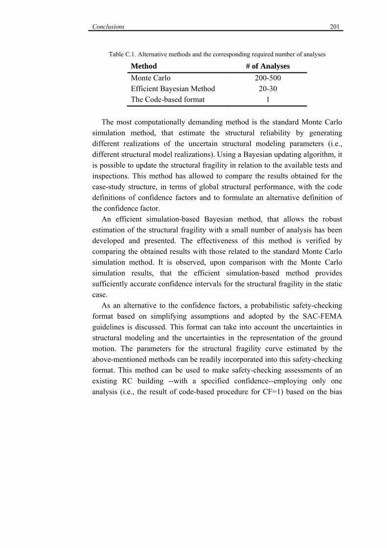
Conclusions 201
Table C.1. Alternative methods and the corresponding required number of analyses
Method # of Analyses Monte Carlo 200-500 Efficient Bayesian Method 20-30 The Code-based format 1
The most computationally demanding method is the standard Monte Carlo
simulation method, that estimate the structural reliability by generating different realizations of the uncertain structural modeling parameters (i.e., different structural model realizations). Using a Bayesian updating algorithm, it is possible to update the structural fragility in relation to the available tests and inspections. This method has allowed to compare the results obtained for the case-study structure, in terms of global structural performance, with the code definitions of confidence factors and to formulate an alternative definition of the confidence factor.
An efficient simulation-based Bayesian method, that allows the robust estimation of the structural fragility with a small number of analysis has been developed and presented. The effectiveness of this method is verified by comparing the obtained results with those related to the standard Monte Carlo simulation method. It is observed, upon comparison with the Monte Carlo simulation results, that the efficient simulation-based method provides sufficiently accurate confidence intervals for the structural fragility in the static case.
As an alternative to the confidence factors, a probabilistic safety-checking format based on simplifying assumptions and adopted by the SAC-FEMA guidelines is discussed. This format can take into account the uncertainties in structural modeling and the uncertainties in the representation of the ground motion. The parameters for the structural fragility curve estimated by the above-mentioned methods can be readily incorporated into this safety-checking format. This method can be used to make safety-checking assessments of an existing RC building --with a specified confidence--employing only one analysis (i.e., the result of code-based procedure for CF=1) based on the bias
202 Conclusions
and the dispersion factors tabulated for different classes of representative existing structures.
For example, these tables and the updated probability distributions, for various KL’s, based on special cases of test and inspection results, are constructed for both static and dynamic non-linear analyses for the case study structure.
Special attention has been focused on seismic record selection and the uncertainty related to the representation of ground motion. In this context, the choice of the parameter (scalar or vector) representative of the ground motion intensity and used in the estimation of the structural performance is fundamental. In order to obtain an assessment of the structural performance which is not affected by the particular choice of the set of records used in the analysis, the representative ground motion parameter adopted as a intensity measure IM, should be both sufficient and efficient. A graphical and statistical tool was implemented in the thesis in order to evaluate the fulfillment of the condition of sufficiency for different intensity measures. When this condition is not verified a simplified method using the weighted regression is employed in order to adjust the structural performance assessment in relation to the observed dependencies. The weights are assigned in relation to the results of the seismic hazard disaggregation for the site of interest.
All the methods proposed within this work are based on the definition of probability distributions for uncertain parameters. The uncertain parameters considered include the materials properties, the construction details parameters and, in the case of dynamic analyses, the uncertainty in the ground motion representation. For each knowledge level, the probability distributions for the uncertain parameters are updated using the Bayesian updating framework. The uncertain parameters are divided in groups (emulating various construction zones). It is assumed that the uncertain parameter belonging to distinct groups are fully un-correlated and only the uncertain parameters inside a given group can be correlated. It should be noted that decisions on possible groupings of the uncertain parameters can affect significantly the global performance assessment of the structure.
Conclusions 203
It should be emphasized that developing prior distributions is probably the most controversial aspect of any Bayesian analysis. Considerable care should be taken when characterizing the prior probability distributions. The process by which priors are selected must be justified carefully. This is because inappropriate choices for priors can lead to incorrect inferences. To this end, with regard to construction details, a survey for professional engineers has been prepared in order to characterize the prior distributions related to expert opinion. This survey is presented in the thesis together with the preliminary testing results obtained by interviewing a small number of structural engineering professionals.
The aim of this work has been to make a step in the direction of implementing probabilistic performance-based methodologies for the assessment of existing RC buildings accessible to engineering professionals and that can, therefore, be adopted by future seismic codes.
For this aim, a range of methods has been proposed in order to allow the engineering professional to choose the most suitable method as a function of the importance of the structure and the level of precision desired.
As future goals, it can be useful to develop a Bayesian adaptive methodology for optimal programming of in-situ tests and inspections for probabilistic seismic assessment of existing buildings for a set of uncertain modelling parameters.
In fact, the Bayesian framework could be used to incorporate the test results in an adaptive manner in order to obtain a sequence of updated probability distributions for the modelling uncertainties affecting the structural performance based on increasing test results. The structural reliability can be also updated as a function of the updated probability distributions. The decision to stop the test would be reached when the structural reliability becomes effectively insensitive to the increasing number of tests.
Appendices 204
Appendices
A. Lumped Plasticity Model
Two main approaches can be used in order to take into account the inelastic behaviour of materials:
• Lumped plasticity model
• Distributed plasticity model
In the present study, it was decided to use the lumped plasticity model that allows concentrating the member non-linear behaviour in correspondence of their ends; such simplification is particularly indicated in the case of frame structures where the potential plastic hinges are located at the member ends.
In fact, in a frame structure, the moment distribution due to the horizontal lateral loads, not taking into account the gravity loads effects, is linear as reported in Figure A.1 and thus, each member can be considered as a fixed-end cantilever member, with a span equal to LV, subjected to a force on the free end.
The length LV is termed as the shear span and it is defined by the distance from the member ends to the inflexion point of the member deformed shape, corresponding to the point in which the moment diagram is equal to zero. The location of the inflexion point can be determined from the linear response of an element to lateral loads. However, once the first plastic regions develop, a redistribution of the flexural moments and a consequent displacement of the
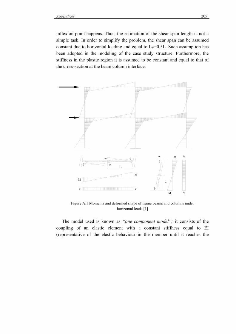
Appendices 205
inflexion point happens. Thus, the estimation of the shear span length is not a simple task. In order to simplify the problem, the shear span can be assumed constant due to horizontal loading and equal to LV=0,5L. Such assumption has been adopted in the modeling of the case study structure. Furthermore, the stiffness in the plastic region it is assumed to be constant and equal to that of the cross-section at the beam column interface.
θ
θ
θ
θ
LV
w
w
MM
V VM
M
V
V
LV
w
Figure A.1 Moments and deformed shape of frame beams and columns under
horizontal loads [1]
The model used is known as “one component model”; it consists of the coupling of an elastic element with a constant stiffness equal to EI (representative of the elastic behaviour in the member until it reaches the
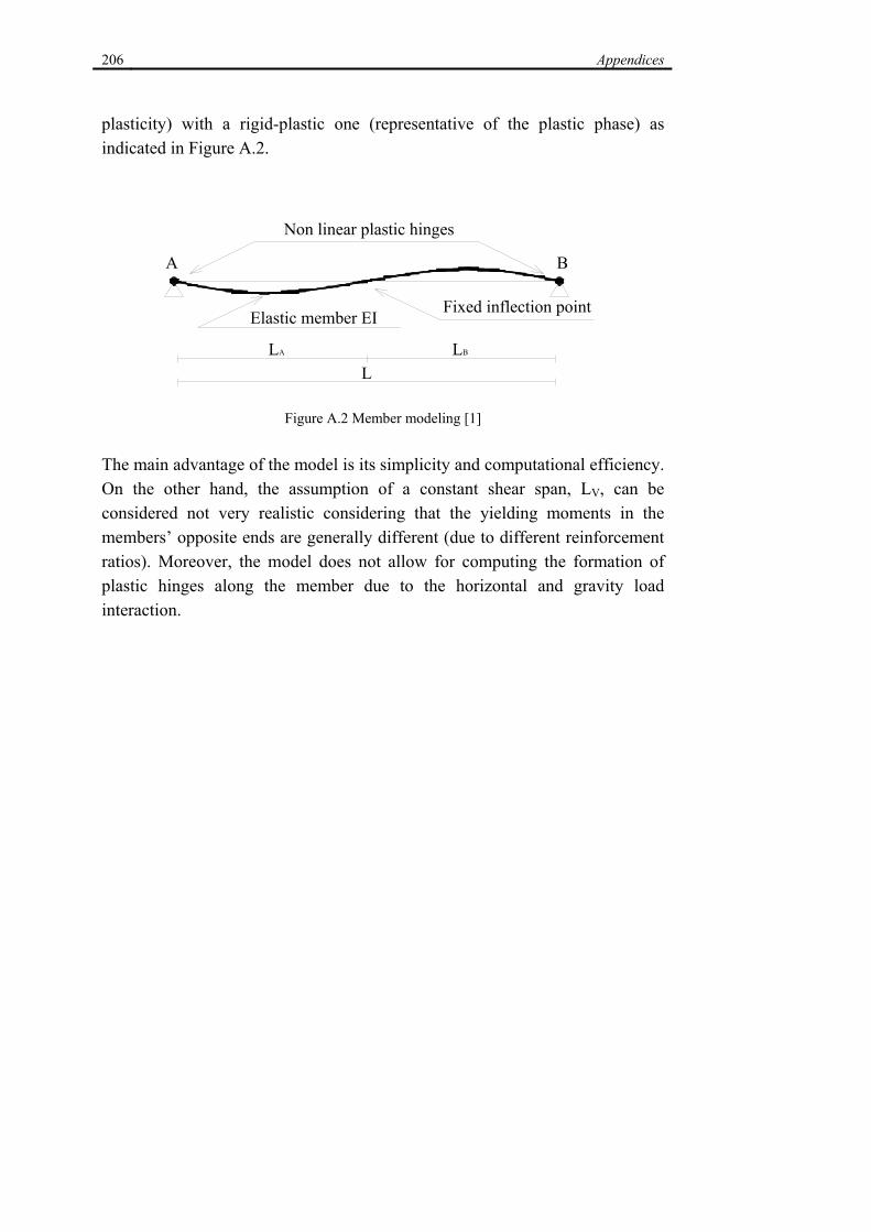
206 Appendices
plasticity) with a rigid-plastic one (representative of the plastic phase) as indicated in Figure A.2.
A B
LA LB
L
Non linear plastic hinges
Elastic member EI Fixed inflection point
Figure A.2 Member modeling [1]
The main advantage of the model is its simplicity and computational efficiency. On the other hand, the assumption of a constant shear span, LV, can be considered not very realistic considering that the yielding moments in the members’ opposite ends are generally different (due to different reinforcement ratios). Moreover, the model does not allow for computing the formation of plastic hinges along the member due to the horizontal and gravity load interaction.
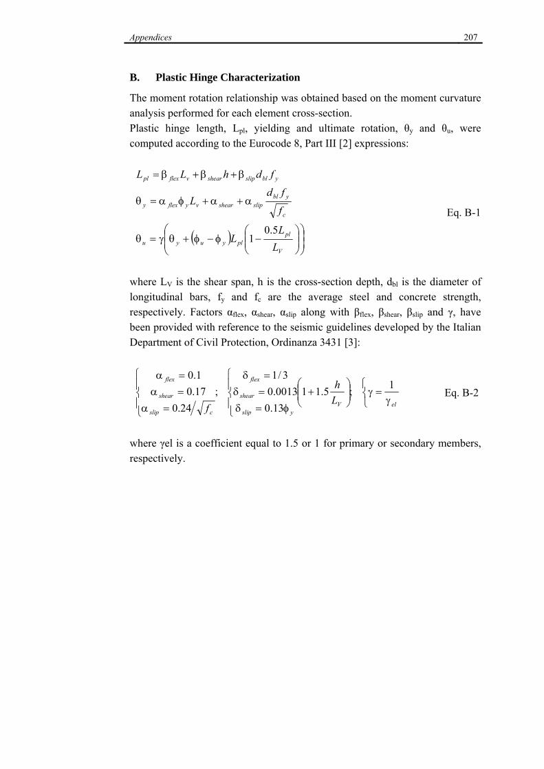
Appendices 207
B. Plastic Hinge Characterization
The moment rotation relationship was obtained based on the moment curvature analysis performed for each element cross-section. Plastic hinge length, Lpl, yielding and ultimate rotation, θy and θu, were computed according to the Eurocode 8, Part III [2] expressions:
( ) ⎟⎟⎠
⎞⎜⎜⎝
⎛⎟⎟⎠
⎞⎜⎜⎝
⎛−φ−φ+θγ=θ
α+α+φα=θ
β+β+β=
V
plplyuyu
c
yblslipshearvyflexy
yblslipshearvflexpl
LL
L
f
fdL
fdhLL
5.01
Eq. B-1
where LV is the shear span, h is the cross-section depth, dbl is the diameter of longitudinal bars, fy and fc are the average steel and concrete strength, respectively. Factors αflex, αshear, αslip along with βflex, βshear, βslip and γ, have been provided with reference to the seismic guidelines developed by the Italian Department of Civil Protection, Ordinanza 3431 [3]:
⎩⎨⎧
γ=γ⎟⎟
⎠
⎞⎜⎜⎝
⎛+
⎪⎩
⎪⎨
⎧
φ=δ=δ=δ
⎪⎩
⎪⎨
⎧
=α=α=α
elVyslip
shear
flex
cslip
shear
flex
Lh
f
1;5.1113.00013.0
3/1;
24.017.01.0
Eq. B-2
where γel is a coefficient equal to 1.5 or 1 for primary or secondary members, respectively.
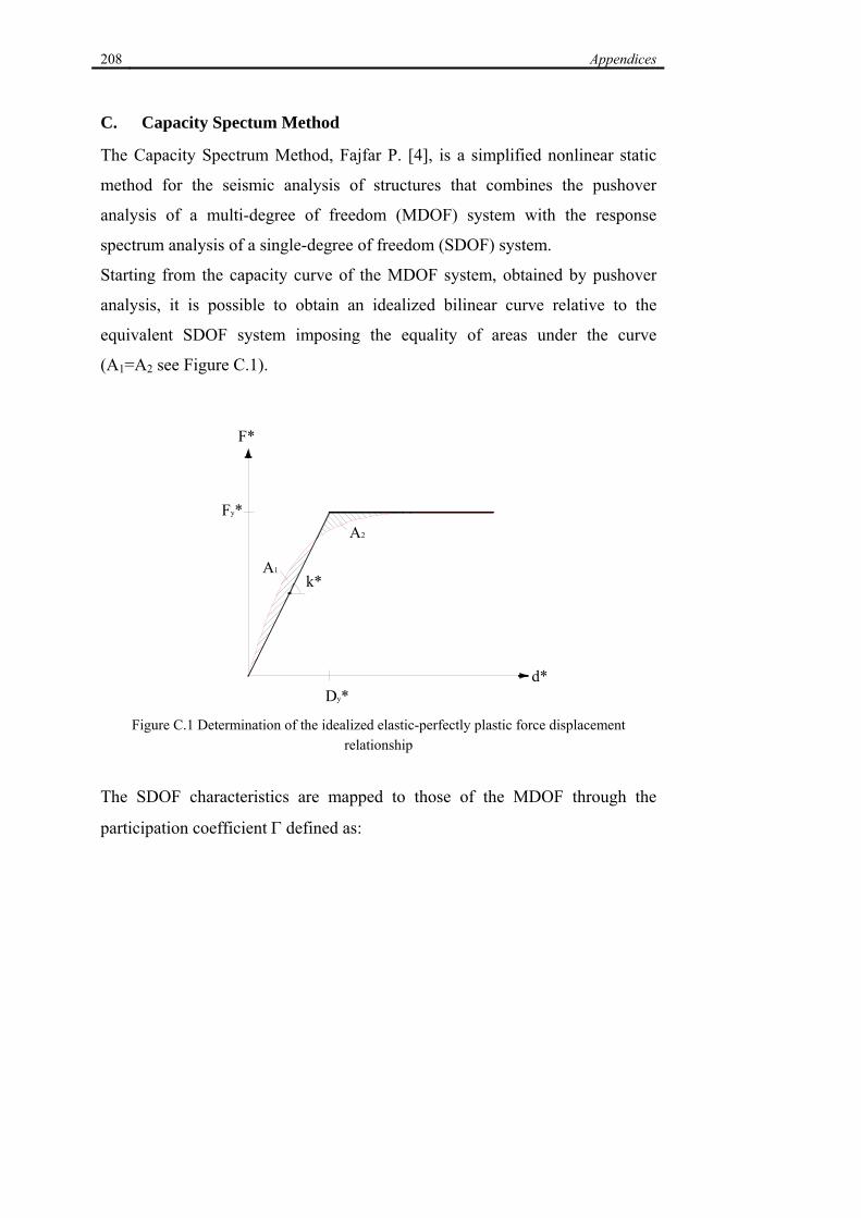
208 Appendices
C. Capacity Spectum Method
The Capacity Spectrum Method, Fajfar P. [4], is a simplified nonlinear static
method for the seismic analysis of structures that combines the pushover
analysis of a multi-degree of freedom (MDOF) system with the response
spectrum analysis of a single-degree of freedom (SDOF) system.
Starting from the capacity curve of the MDOF system, obtained by pushover
analysis, it is possible to obtain an idealized bilinear curve relative to the
equivalent SDOF system imposing the equality of areas under the curve
(A1=A2 see Figure C.1).
F*
d*
Fy*
Dy*
k*
A2
A1
Figure C.1 Determination of the idealized elastic-perfectly plastic force displacement
relationship
The SDOF characteristics are mapped to those of the MDOF through the
participation coefficient Γ defined as:
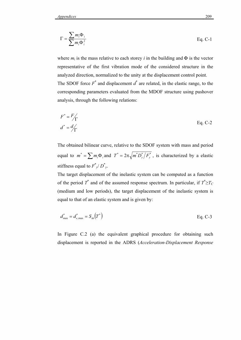
Appendices 209
∑∑
Φ
Φ=Γ 2
ii
ii
mm
Eq. C-1
where mi is the mass relative to each storey i in the building and Φ is the vector
representative of the first vibration mode of the considered structure in the
analyzed direction, normalized to the unity at the displacement control point.
The SDOF force F* and displacement d* are related, in the elastic range, to the
corresponding parameters evaluated from the MDOF structure using pushover
analysis, through the following relations:
Γ= FF *
Γ= dd * Eq. C-2
The obtained bilinear curve, relative to the SDOF system with mass and period
equal to iimm Φ= ∑* and **** 2 yy FDmT π= , is characterized by a elastic
stiffness equal to F*y/ D*
y.
The target displacement of the inelastic system can be computed as a function
of the period T* and of the assumed response spectrum. In particular, if T*≥TC
(medium and low periods), the target displacement of the inelastic system is
equal to that of an elastic system and is given by:
( )**max,
*max TSdd dee == Eq. C-3
In Figure C.2 (a) the equivalent graphical procedure for obtaining such
displacement is reported in the ADRS (Acceleration-Displacement Response
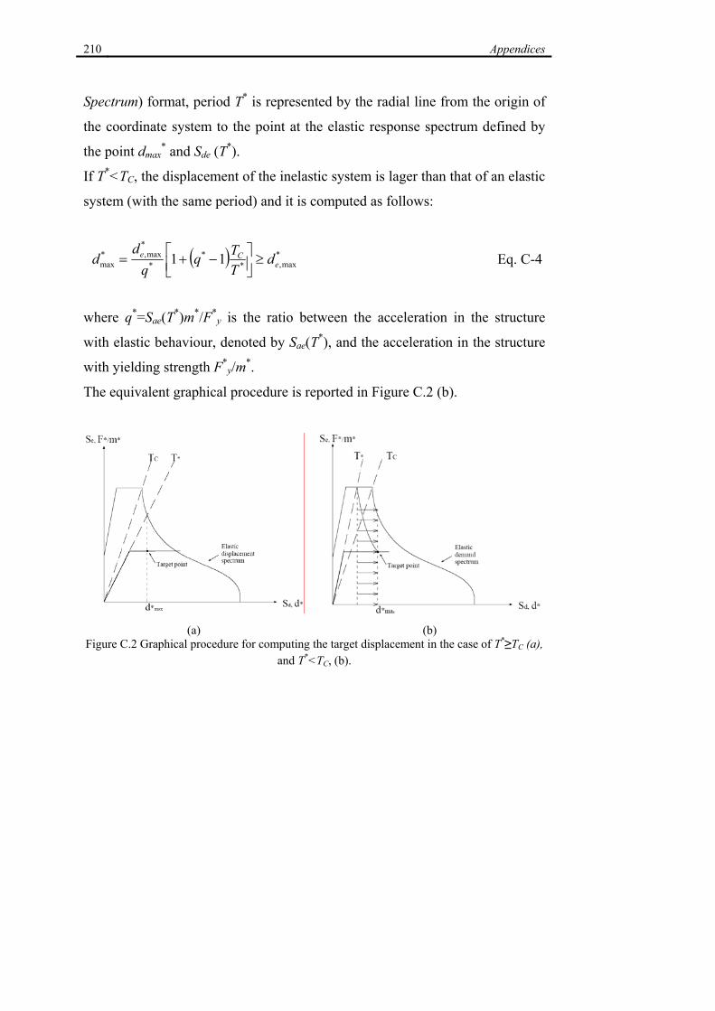
210 Appendices
Spectrum) format, period T* is represented by the radial line from the origin of
the coordinate system to the point at the elastic response spectrum defined by
the point dmax* and Sde (T*).
If T*<TC, the displacement of the inelastic system is lager than that of an elastic
system (with the same period) and it is computed as follows:
( ) *max,*
**
*max,*
max 11 eCe d
TTq
qd
d ≥⎥⎦⎤
⎢⎣⎡ −+= Eq. C-4
where q*=Sae(T*)m*/F*y is the ratio between the acceleration in the structure
with elastic behaviour, denoted by Sae(T*), and the acceleration in the structure
with yielding strength F*y/m*.
The equivalent graphical procedure is reported in Figure C.2 (b).
(a) (b)
Figure C.2 Graphical procedure for computing the target displacement in the case of T*≥TC (a), and T*<TC, (b).

Appendices 211
Once the target displacement for the equivalent SDOF system has been
computed, the target displacement of the MDOF system is given by:
*maxmax dd ⋅Γ= Eq. C-5
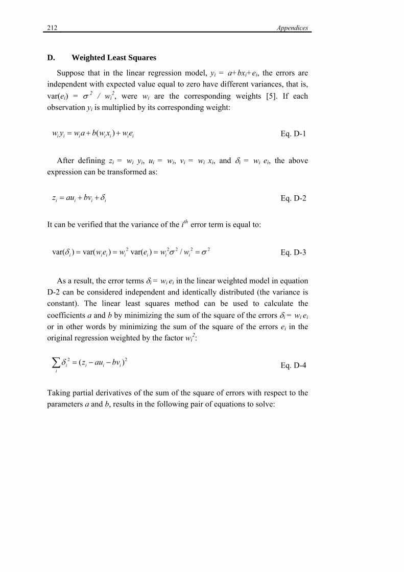
212 Appendices
D. Weighted Least Squares
Suppose that in the linear regression model, yi = a+bxi+ei, the errors are independent with expected value equal to zero have different variances, that is, var(ei) = σ 2 / wi
2, were wi are the corresponding weights [5]. If each observation yi is multiplied by its corresponding weight:
( )i i i i i i iw y w a b w x w e= + + Eq. D-1
After defining zi = wi yi, ui = wi, vi = wi xi, and δi = wi ei, the above
expression can be transformed as:
i i i iz au bv δ= + + Eq. D-2
It can be verified that the variance of the ith error term is equal to:
2 2 2 2 2var( ) var( ) var( ) /i i i i i i iw e w e w wδ σ σ= = = = Eq. D-3
As a result, the error terms δi = wi ei in the linear weighted model in equation
D-2 can be considered independent and identically distributed (the variance is constant). The linear least squares method can be used to calculate the coefficients a and b by minimizing the sum of the square of the errors δi = wi ei or in other words by minimizing the sum of the square of the errors ei in the original regression weighted by the factor wi
2:
2 2( )i i i ii
z au bvδ = − −∑ Eq. D-4
Taking partial derivatives of the sum of the square of errors with respect to the parameters a and b, results in the following pair of equations to solve:
Appendices 213
2
2
2 ( ) 0
2 ( ) 0
ii
i i i ii
ii
i i i ii
u z au bva
v z au bvb
δ
δ
∂= − − − =
∂
∂= − − − =
∂
∑∑
∑∑
Eq. D-5
Therefore, the coefficients a and b can be calculated as:
∑∑
∑∑∑ ∑ ∑
∑ ∑ ∑
−=
−
−=
22
222
222
)()()()()()(
i
ii
i
ii
iiii
iiiii
u
vub
u
zua
vuvuzvuzu
b
Eq. D-6
After substituting zi = wi yi, ui = wi, vi = wi xi, the expressions for coefficients a and b for the weighted regression model can be written as:
∑∑
∑∑
∑ ∑ ∑∑ ∑ ∑
−=
−
−=
2
2
2
2
2222
22222
)()()(
)()()(
i
ii
i
ii
iiiii
iiiiii
w
xwb
w
ywa
ywwyw
yxwwywb
Eq. D-7
And the sum of the square of the errors of the weighted regression will be equal to:
2222 )()( iiiiii bxaywews −−=== ∑∑∑δ Eq. D-8
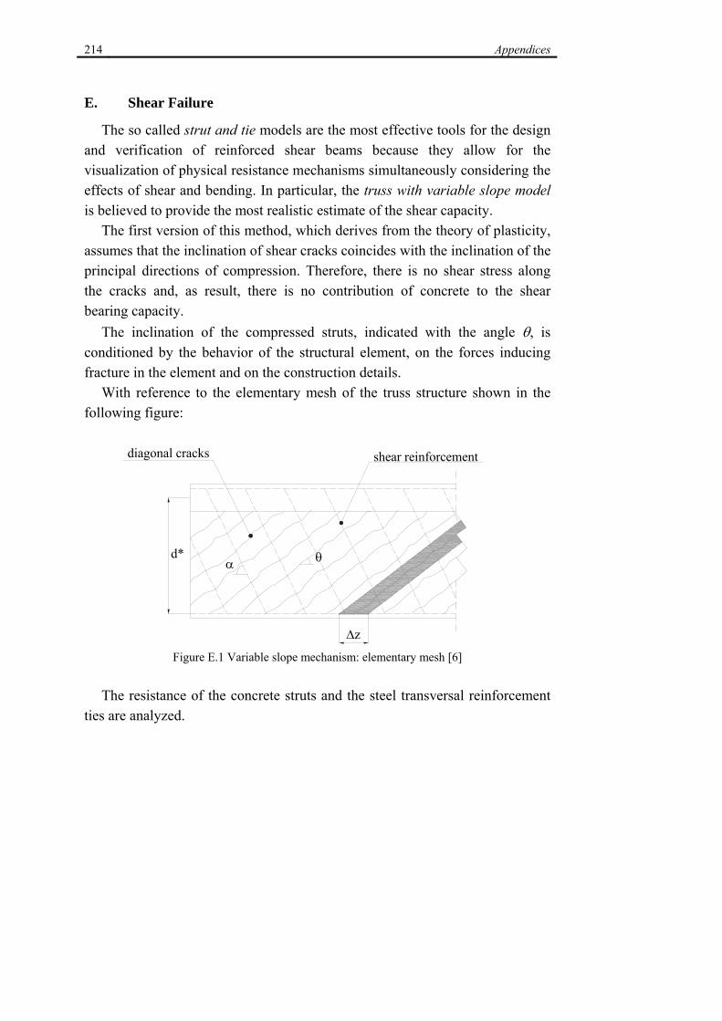
214 Appendices
E. Shear Failure
The so called strut and tie models are the most effective tools for the design and verification of reinforced shear beams because they allow for the visualization of physical resistance mechanisms simultaneously considering the effects of shear and bending. In particular, the truss with variable slope model is believed to provide the most realistic estimate of the shear capacity.
The first version of this method, which derives from the theory of plasticity, assumes that the inclination of shear cracks coincides with the inclination of the principal directions of compression. Therefore, there is no shear stress along the cracks and, as result, there is no contribution of concrete to the shear bearing capacity.
The inclination of the compressed struts, indicated with the angle θ, is conditioned by the behavior of the structural element, on the forces inducing fracture in the element and on the construction details.
With reference to the elementary mesh of the truss structure shown in the following figure:
θα
∆z
d*
diagonal cracks shear reinforcement
Figure E.1 Variable slope mechanism: elementary mesh [6]
The resistance of the concrete struts and the steel transversal reinforcement
ties are analyzed.
Appendices 215
The crisis of the compressed strut happens when the following equation is satisfied:
( ) cdccdccd zbtbS σ⋅ν⋅α⋅θ⋅∆⋅=σ⋅ν⋅α⋅⋅= sin Eq. E-1
where:
θ⋅∆= sinzt Eq. E-2
The coefficient ν takes into account the real distribution of stresses along the strut (which is actually inflected). The Italian code requires ν = 0.50. The coefficient αc takes into account the presence of axial compression forces. The Italian code characterizes αc as the following: • 1=α c for uncompressed element
• cdcpc σσ+=α 1 for 25.00 <σ≤ cp
• 25.1=α c for cdcpcd σ≤σ≤σ 50.025.0
• ( )cdcpc σσ−=α 150.2 for cdcpcd σ≤σ≤σ50.0
Eq. E-3
where σcp is the average stress of compression.
If we zoom into the elementary mesh outlined in the following figure:
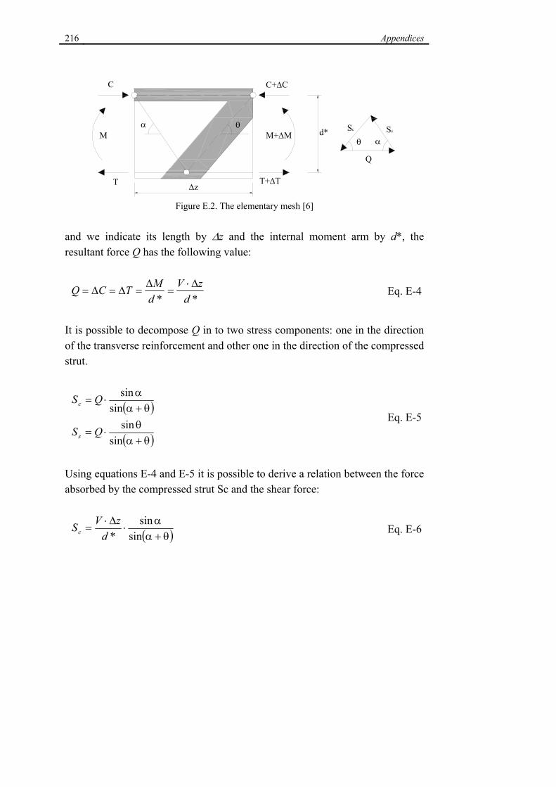
216 Appendices
d*
C+∆CC
T T+∆T
M+∆MMθα
Q
Sc Ss
θ α
∆z
Figure E.2. The elementary mesh [6] and we indicate its length by ∆z and the internal moment arm by d*, the resultant force Q has the following value:
** dzV
dMTCQ ∆⋅
=∆
=∆=∆= Eq. E-4
It is possible to decompose Q in to two stress components: one in the direction of the transverse reinforcement and other one in the direction of the compressed strut.
( )
( )θ+αθ
⋅=
θ+αα
⋅=
sinsin
sinsin
QS
QS
s
c
Eq. E-5
Using equations E-4 and E-5 it is possible to derive a relation between the force absorbed by the compressed strut Sc and the shear force:
( )θ+αα
⋅∆⋅
=sin
sin*d
zVSc Eq. E-6
Appendices 217
By setting equation E-1 equal to equation E-6, one can obtain the critical shear value in the compressed strut:
( )( )
θ+θ+α
⋅σ⋅α⋅ν⋅⋅=⇒
⇒θ+α⋅θ⋅σ⋅α⋅ν⋅⋅=⇒
⇒θ+α
α⋅
∆⋅==σ⋅ν⋅α⋅θ⋅∆⋅=
2
2
cot1cotcot*
cotcotsin*sin
sin*
sin
cdcRcd
cdcRcd
Rcdccdccd
dbV
dbVd
zVSzbS
Eq. E-7
Considering that only vertical stirrups (α=90°) are present in the element, the equation E-7 becomes:
θ+θ⋅σ⋅α⋅ν⋅⋅=
tancot1* cdcRcd dbV Eq. E-8
It should be noted that the maximum shear resistance corresponds to θ = 45°. If the external shear force is less then the maximum shear resistance, calculated for θ = 45°, the equilibrium in Figure 4 can be achieved for θ values less than 45°.
In the same manner, critical axial force in the transverse reinforcement is reached on the onset of yielding:
ydswsd fS ⋅Ω= Eq. E-9
where Ωsw is the total area of the reinforcement present in the length ∆z. If the area of the single transverse reinforcement rebar is indicated with Asw, we have:
szAswsw
∆=Ω Eq. E-10
where s is the transverse reinforcement spacing.
218 Appendices
Using equations E-4 and E-5, one can derive a relation between the axial force in the transverse reinforcement Ss and the shear force V:
( )θ+αθ
⋅∆⋅
=sin
sin*d
zVSs Eq. E-11
By setting equation D-8 equal to equation D-11, we can obtain the shear critical force that corresponds to the yielding of the transverse reinforcement:
( )
( )θ+α⋅α⋅⋅⋅=⇒
⇒θ+α
θ⋅
∆⋅==⋅
∆⋅=
cotcotsin*sin
sin*
sdfAV
dzV
Sfs
zAS
ydswRsd
Rsdsyd
swsd
Eq. E-12
Considering that only vertical stirrups (α=90°) are present, the equation becomes:
θ⋅⋅⋅= cot*s
dfAV ydswRsd Eq. E-13
It should be noted, from the previous equation, that the shear resistance decreases with the increasing slope angle θ.
The Italian code limits that the inclination θ of the concrete struts with the beam axis in the following interval:
°≥θ≥°⇒≤θ≤ 81.21455.2cot1 Eq. E-14
Appendices 219
References
[1] Verderame, G., “Analisi sismica di edifici in C.A. progettati per carichi gravitazionali,” PhD. Thesis,, XII ciclo, 1999.
[2] CEN, European Committee for Standardisation TC250/SC8/ [2003] “Eurocode 8: Design Provisions for Earthquake Resistance of Structures, Part 1.1: General rules, seismic actions and rules for buildings,” PrEN1998-1.
[3] Ordinanza del Presidente del Consiglio dei Ministri (OPCM) n. 3431, “Ulteriori modifiche ed integrazioni all'ordinanza del Presidente del Consiglio dei Ministri n. 3274 del 20 marzo 2003”. Gazzetta Ufficiale della Repubblica Italiana n. 107 del 10-5-2005 (Suppl. Ordinario n.85), 2005 (in Italian).
[4] Fajfar, P. “Capacity spectrum method based on inelastic demand spectra”, Earthquake Engineering and Structural Dynamics; 28:979–93, 1999.
[5] Rice J. A., (1995) Mathematical Statistics and Data Analysis, Belmont, CA: Duxbury/Wadsworth.
[6] Cosenza E., Manfredi G., Pecce M., Strutture in cemento armato – basi della progettazione. Hoepli, 2008.
![ŞTIR] NOU DIĂ N DACIA MALVEMS...» XXL—Memoriile Sceţiunii Istorice 6.— » XXII, - Desbaterile în 18519—190 0 Academie6.i ¬ ... unei cultur intensivi greco-romane de pest](https://static.fdocument.org/doc/165x107/5f7e6f5e28ac701a82745572/tir-nou-di-n-dacia-xxlamemoriile-sceiunii-istorice-6a-xxii.jpg)