Optimization techniques for a model problem of saltwater intrusion in coastal aquifers

1

Applied Math and Computers Lab Department of Sciences

Technical University of Crete

24/6/2014

P.N. Stratis, E.P. Papadopoulou, M.S. Zakynthinaki

and Y.G. Saridakis

This research has been co-financed by the European Union (European Social Fund – ESF) and Greek national funds through the Operational Program "Education and Lifelong Learning" of the National Strategic Reference Framework (NSRF) - Research Funding Program: THALIS. Investing in knowledge society through the European Social Fund.

Presentation contents

• Part 1. Saltwater intrusion • Part 2. Mathematical approach-model equations • Part 3. Types of coastal freshwater aquifers • Part 4. Pumping optimization methods • Part 5. Numerical simulations

2 24/6/2014

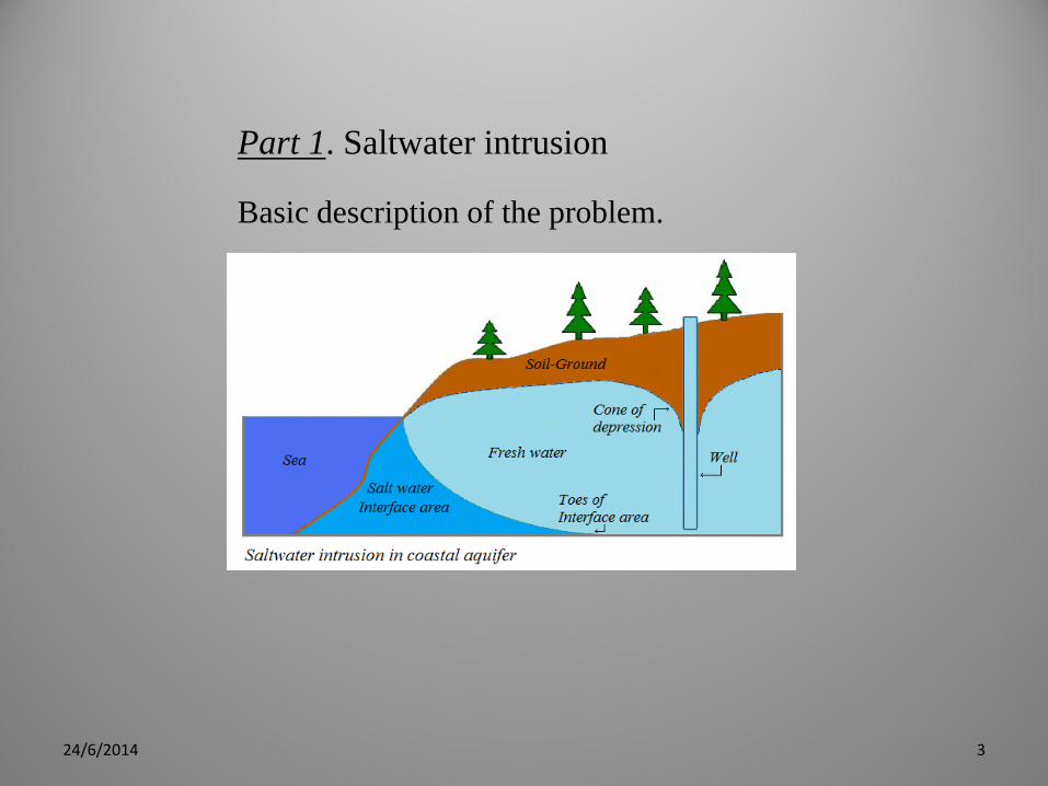
Part 1. Saltwater intrusion

Basic description of the problem.

3 24/6/2014

The problem: Rapidly increasing needs for fresh water in coastal areas and islands, due to: Population growth Tourism Agriculture needs

results to: • Intensive pumping in freshwater aquifers, mostly during

summer months, beyond the tolerable limits of their natural replenishment.

4 24/6/2014

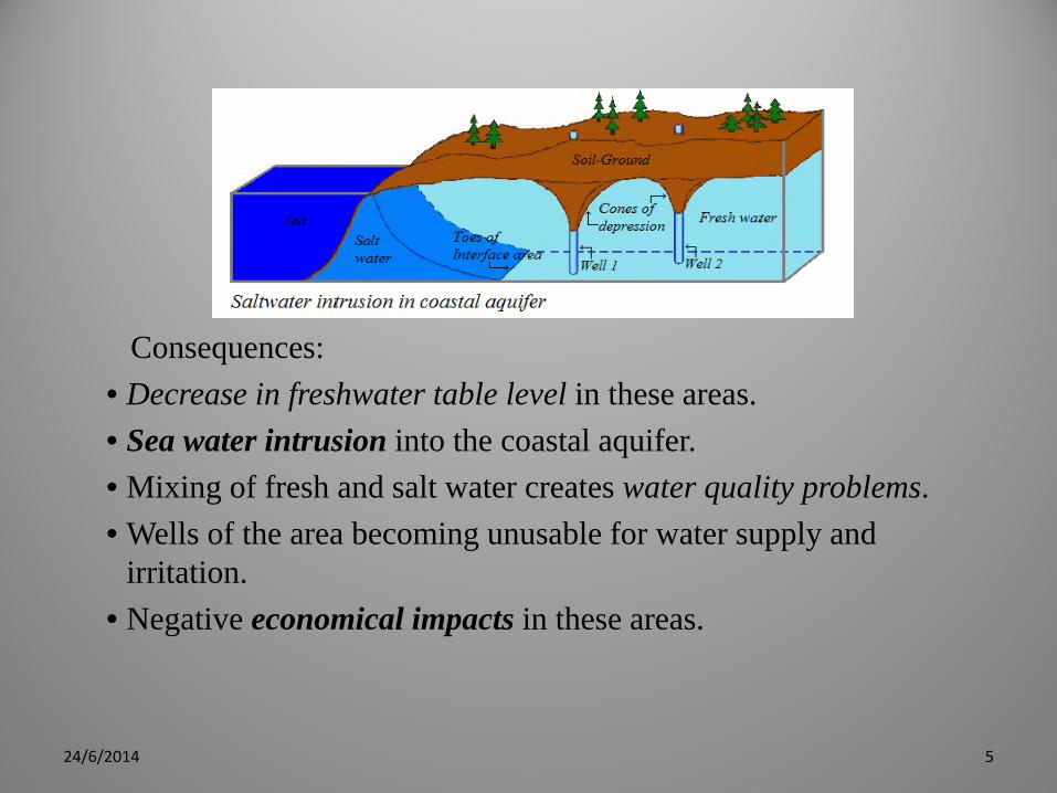
Consequences: • Decrease in freshwater table level in these areas. • Sea water intrusion into the coastal aquifer. • Mixing of fresh and salt water creates water quality problems. • Wells of the area becoming unusable for water supply and

irritation. • Negative economical impacts in these areas.

5 24/6/2014

There is a great need for developing pumping management methodologies, in order to determine:

• the total volume of water that can be pumped from coastal aquifers,

while protecting the wells from saltwater intrusion.

• the optimal places where wells can be placed, in order to maximize the non-risk pumping of fresh water.

• the max number of wells that can be distributed over the aquifer.

6 24/6/2014

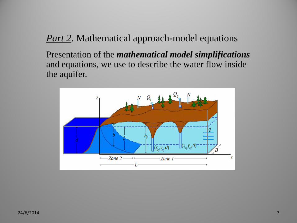
Part 2. Mathematical approach-model equations Presentation of the mathematical model simplifications and equations, we use to describe the water flow inside the aquifer.

7 24/6/2014

Model simplifications

Flow in coastal aquifers is a very complex process, because • there exist more than one mixing fluid phases, • fluid density depends on the unknown concentrations, • there exist a great spatial variability of hydraulic parameters

inside the region of the aquifer. So, model simplifications are needed, in order to provide

reasonable approximate predictions. The most common of them are:

• Sharp Interface approximation, • Ghyben-Herzberg equation.

8 24/6/2014

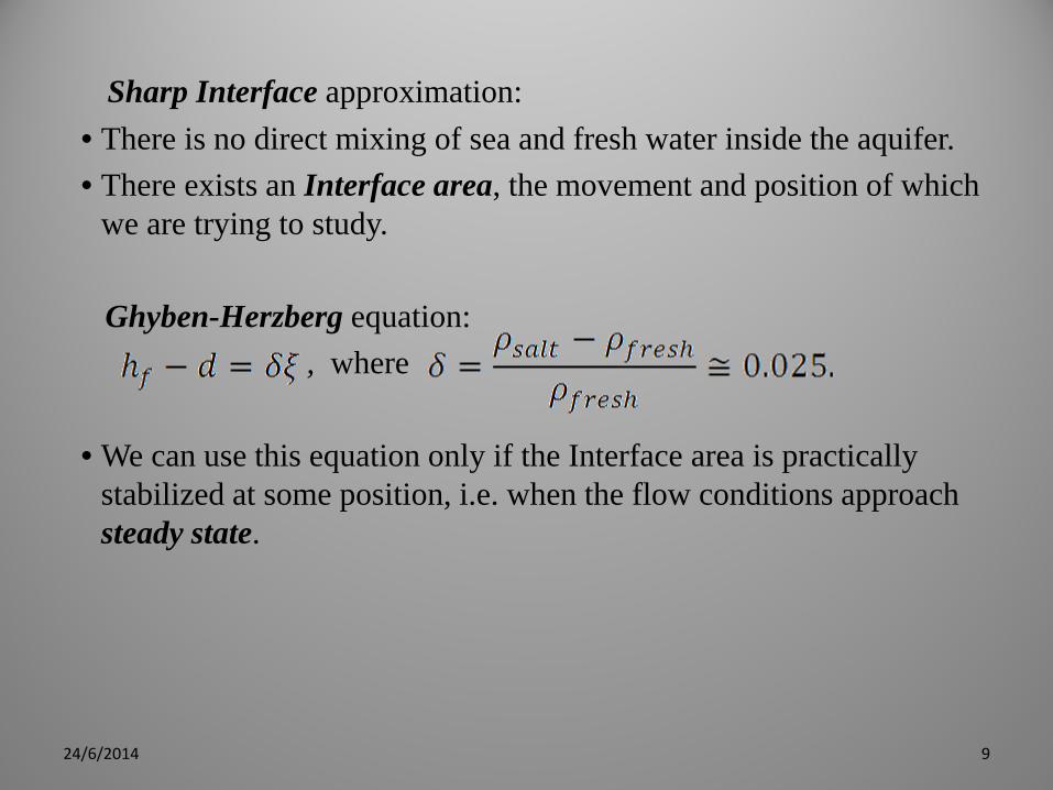
Sharp Interface approximation: • There is no direct mixing of sea and fresh water inside the aquifer. • There exists an Interface area, the movement and position of which

we are trying to study. Ghyben-Herzberg equation: , where • We can use this equation only if the Interface area is practically

stabilized at some position, i.e. when the flow conditions approach steady state.

9 24/6/2014

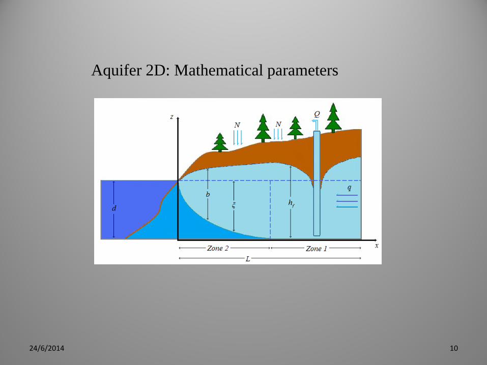
Aquifer 2D: Mathematical parameters

10 24/6/2014

Parameters of the aquifer (distances)

• L: Length of the aquifer.

• B: Width of the aquifer.

• d: Height of the aquifer from its bottom to sea level.

• b(x,y): Freshwater depth from free surface to the Interface.

• ξ(x,y): Freshwater depth from the sea level to the Interface.

• hf(x,y): Freshwater piezometric head with reference to the bottom of the aquifer.

11 24/6/2014

Parameters of the aquifer (areas and water movement)

• τ: Points where the interface surface intersects the base of the aquifer (Toes area).

• Q (m3/day): Pumping rates of the aquifer wells.

• Ν (mm/year): Water recharge distributed over the surface of the aquifer (e.g. rain, rivers).

• Κ (m/day): Hydraulic conductivity.

• q (m2/day): Ambient horizontal discharge per unit width of the aquifer.

12 24/6/2014

Equations:

• Zone 1. Steady flow equation:

where hf = b. • Zone 2. Steady flow equation:

where hf = b+d-ξ.

13 24/6/2014

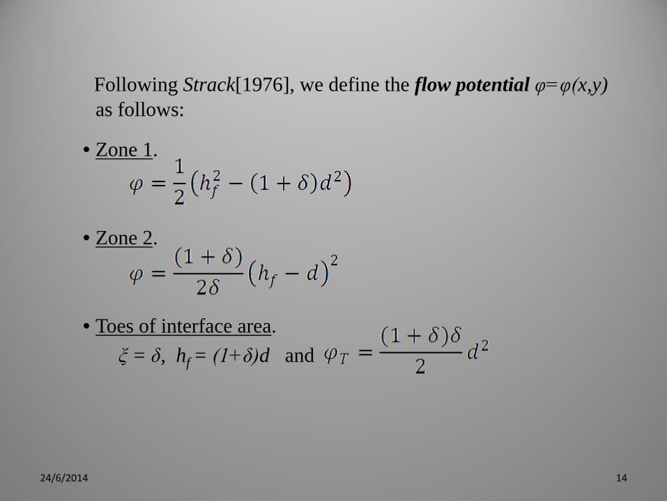
Following Strack[1976], we define the flow potential φ=φ(x,y) as follows:

• Zone 1. • Zone 2.

• Toes of interface area. ξ = δ, hf = (1+δ)d and

14 24/6/2014

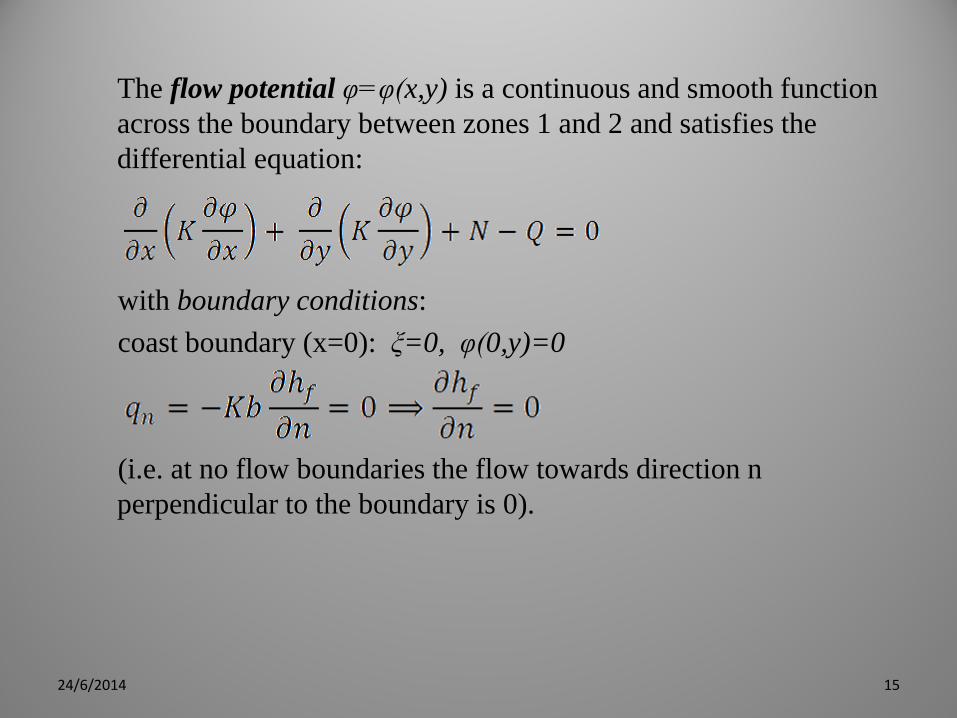
The flow potential φ=φ(x,y) is a continuous and smooth function across the boundary between zones 1 and 2 and satisfies the differential equation:

with boundary conditions: coast boundary (x=0): ξ=0, φ(0,y)=0 (i.e. at no flow boundaries the flow towards direction n

perpendicular to the boundary is 0).

15 24/6/2014

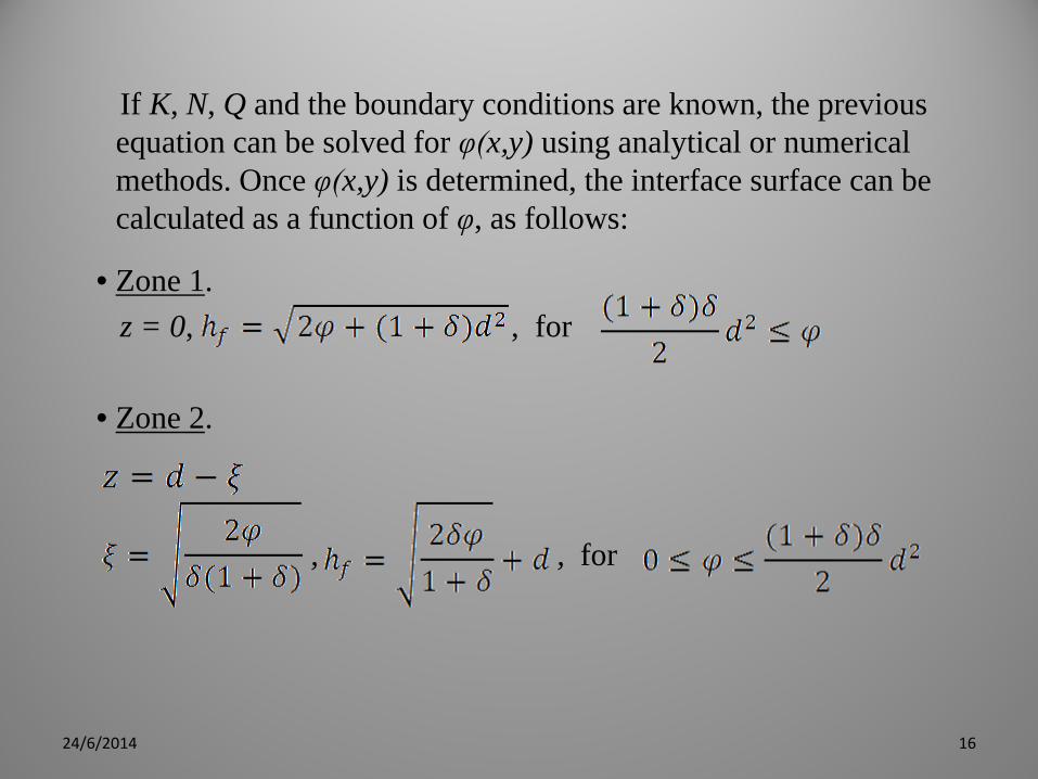
If K, N, Q and the boundary conditions are known, the previous equation can be solved for φ(x,y) using analytical or numerical methods. Once φ(x,y) is determined, the interface surface can be calculated as a function of φ, as follows:

• Zone 1. z = 0, , for • Zone 2. , , for

16 24/6/2014

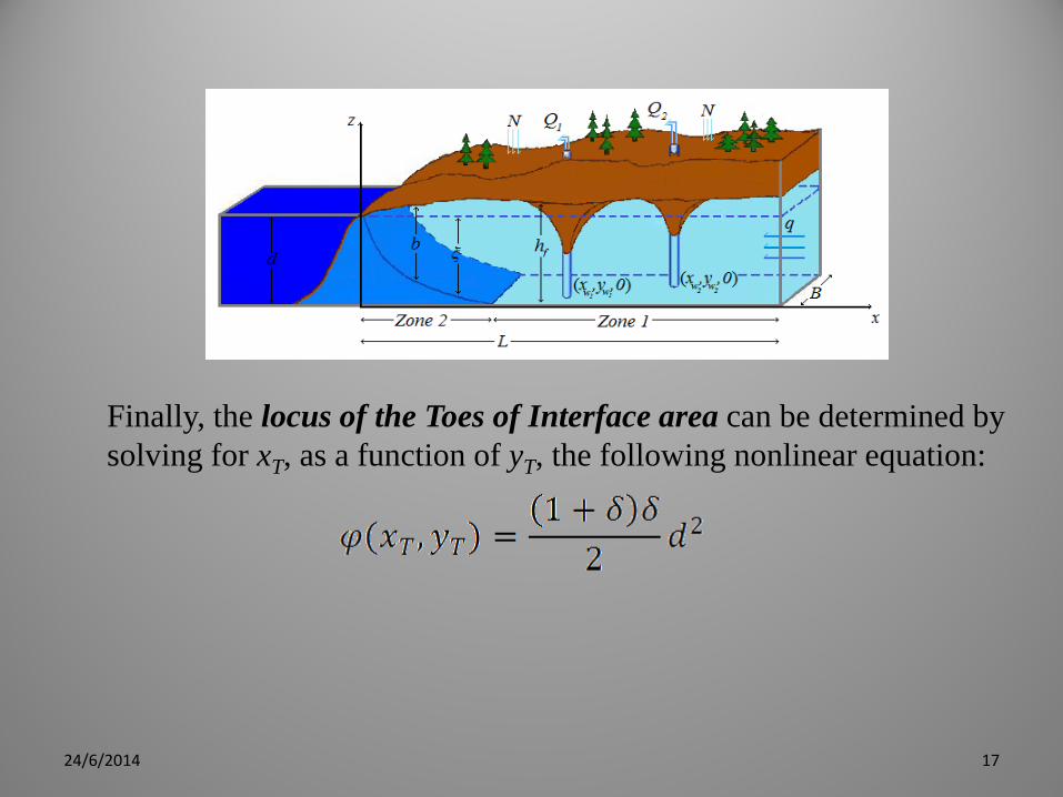
Finally, the locus of the Toes of Interface area can be determined by solving for xT, as a function of yT, the following nonlinear equation:

17 24/6/2014

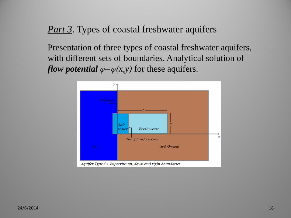
Part 3. Types of coastal freshwater aquifers

Presentation of three types of coastal freshwater aquifers, with different sets of boundaries. Analytical solution of flow potential φ=φ(x,y) for these aquifers.

18 24/6/2014

19 24/6/2014

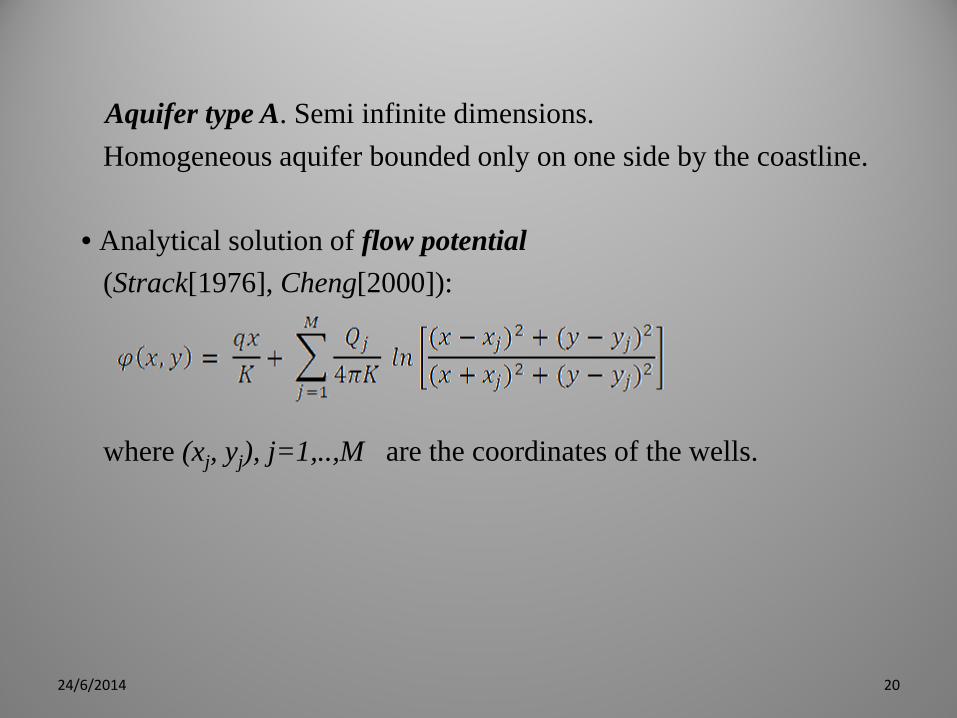
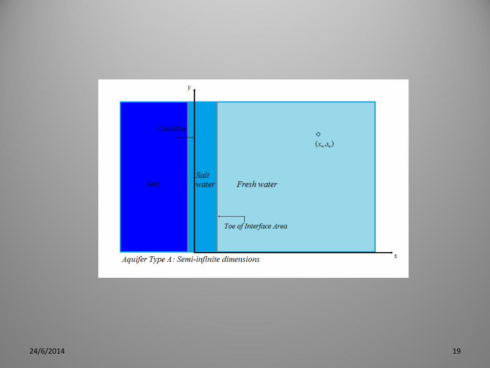
Aquifer type A. Semi infinite dimensions. Homogeneous aquifer bounded only on one side by the coastline. • Analytical solution of flow potential (Strack[1976], Cheng[2000]): where (xj, yj), j=1,..,M are the coordinates of the wells.

20 24/6/2014

21 24/6/2014

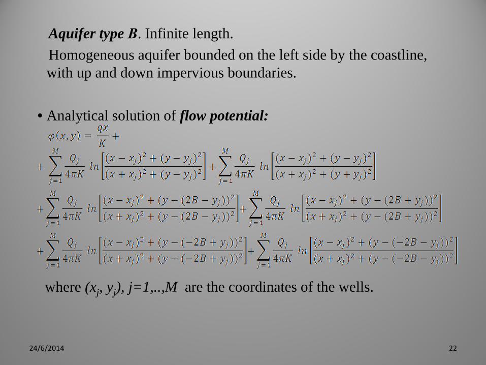
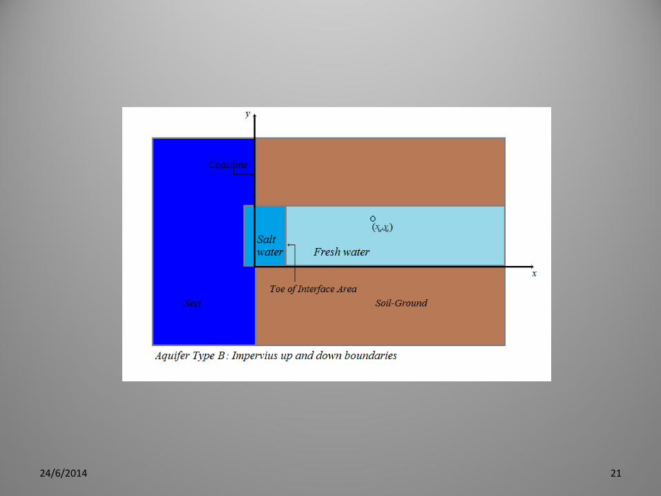
Aquifer type Β. Infinite length. Homogeneous aquifer bounded on the left side by the coastline,

with up and down impervious boundaries. • Analytical solution of flow potential: where (xj, yj), j=1,..,M are the coordinates of the wells.

22 24/6/2014

23 24/6/2014

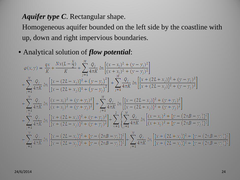
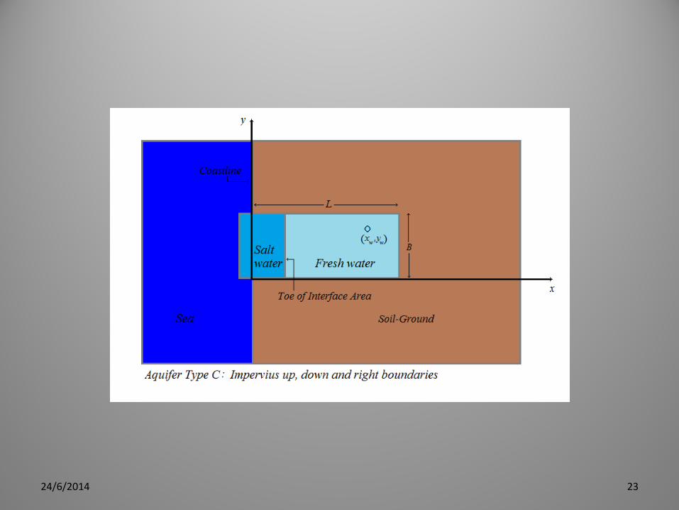
Aquifer type C. Rectangular shape. Homogeneous aquifer bounded on the left side by the coastline with up, down and right impervious boundaries.

• Analytical solution of flow potential:

24 24/6/2014

25

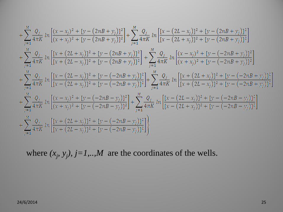
where (xj, yj), j=1,..,M are the coordinates of the wells.

24/6/2014

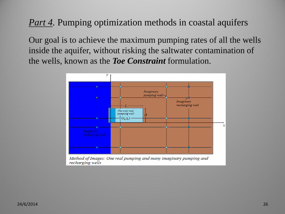
Part 4. Pumping optimization methods in coastal aquifers

Our goal is to achieve the maximum pumping rates of all the wells inside the aquifer, without risking the saltwater contamination of the wells, known as the Toe Constraint formulation.

26 24/6/2014

AL.O.P.EX. method (ALgorithm Of Pattern EXtraction)

• Introduced by Harth και Tzanakou, Syracuse University, 1974. • Stochastic optimization for adaptive correction of atmospheric

distortion in astronomical observation, M. Zakynthinaki, PhD Thesis, Chania, 2001.

• Stochastic optimization algorithm. • Control (cost-profit) function f=f(x1,x2,x3,x4,..,xn). • Goal: Maximize or minimize the control function. • Local extrema can be avoided by the use of some kind of noise.

27 24/6/2014

A few words about the ALOPEX method

• Iterative algorithm. • Every iteration starts with the data of the previous one. • In every iteration all the control variables of the cost function can be

changed simultaneously. • The new values of the variables are stochastically depended from

the change of the cost function between two iterations. • The stochastic element of the procedure is the noise, which is

controlled from the user.

28 24/6/2014

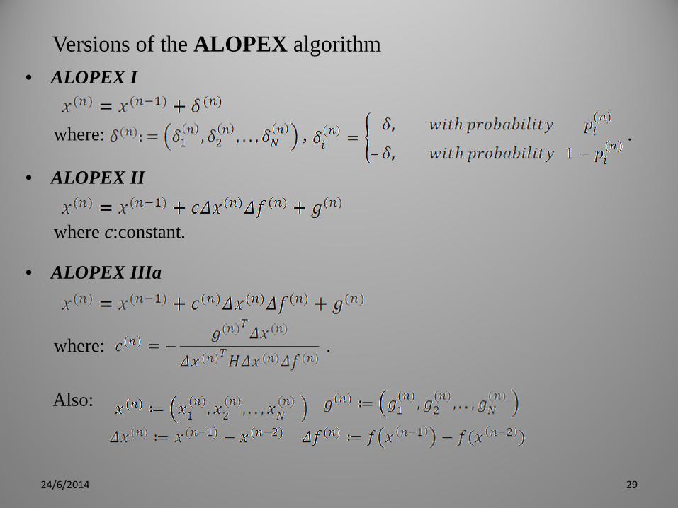
Versions of the ALOPEX algorithm • ALOPEX I where: , .

• ALOPEX II where c:constant.

• ALOPEX IIIa

where: . Also:

29 24/6/2014

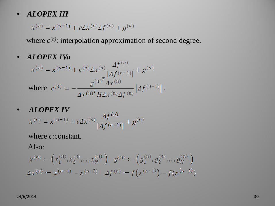
• ALOPEX III

where c(n): interpolation approximation of second degree.

• ALOPEX IVa

where . • ALOPEX IV

where c:constant. Also:

30 24/6/2014

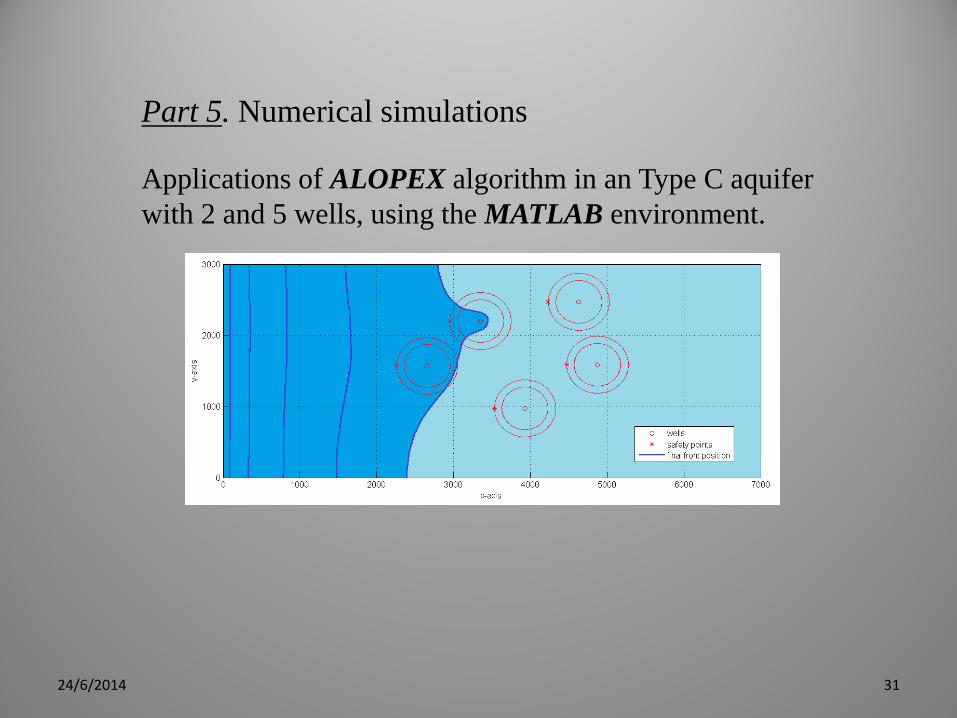
Part 5. Numerical simulations

Applications of ALOPEX algorithm in an Type C aquifer with 2 and 5 wells, using the MATLAB environment.

31 24/6/2014

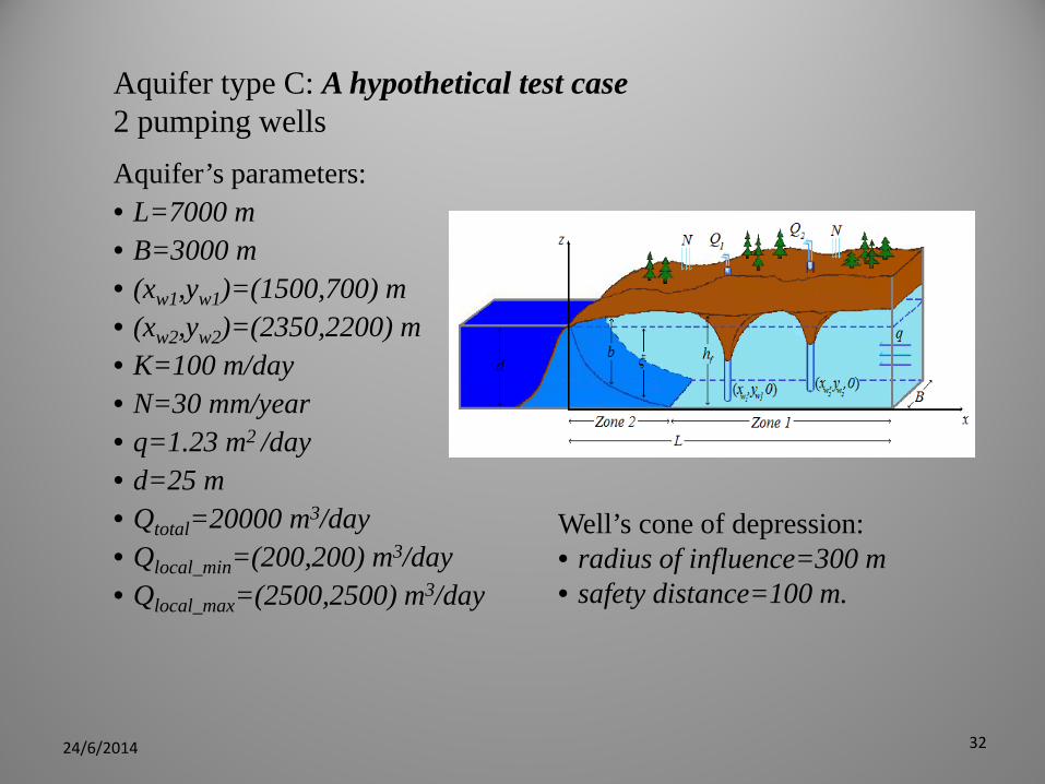
Aquifer type C: A hypothetical test case 2 pumping wells Aquifer’s parameters: • L=7000 m • B=3000 m • (xw1,yw1)=(1500,700) m • (xw2,yw2)=(2350,2200) m • K=100 m/day • N=30 mm/year • q=1.23 m2 /day • d=25 m • Qtotal=20000 m3/day • Qlocal_min=(200,200) m3/day • Qlocal_max=(2500,2500) m3/day

32 24/6/2014

Well’s cone of depression: • radius of influence=300 m • safety distance=100 m.

Algorithm parameters: • c=0.6: acceleration factor • noise(i)(k)=0.05*Q(i)(k)*rand.

24/6/2014 33

ALOPEX II algorithm:

and Profit function:

at k-th iteration.

Penalties management: • Qlocal_min penalty=1.20 • Qlocal_max penalty=0.95 • x-movement penalty=0.95 • critical-distance penalty=0.95.

Q(i)(k)=Q(i)(k-1)+c*[Q(i)(k-1)- Q(i)(k-2)]*[Profit(k-1)- Profit(k-2)]+noise(k)

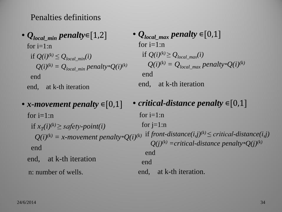
Penalties definitions

• Qlocal_min penalty∊[1,2] for i=1:n if Q(i)(k) ≤ Qlocal_min(i) Q(i)(k) = Qlocal_min penalty*Q(i)(k) end end, at k-th iteration

24/6/2014 34

• Qlocal_max penalty ∊[0,1] for i=1:n if Q(i)(k) ≥ Qlocal_max(i) Q(i)(k) = Qlocal_max penalty*Q(i)(k) end end, at k-th iteration

• x-movement penalty ∊[0,1] for i=1:n if xT(i)(k) ≥ safety-point(i) Q(i)(k) = x-movement penalty*Q(i)(k) end end, at k-th iteration

• critical-distance penalty ∊[0,1] for i=1:n for j=1:n if front-distance(i,j)(k) ≤ critical-distance(i,j) Q(j)(k) =critical-distance penalty*Q(j)(k) end end end, at k-th iteration.

n: number of wells.

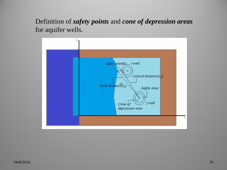
Definition of safety points and cone of depression areas for aquifer wells.

24/6/2014 35

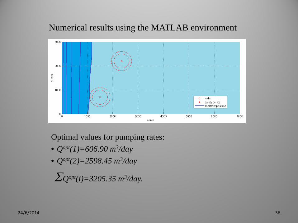
Numerical results using the MATLAB environment

Optimal values for pumping rates: • Qopt(1)=606.90 m3/day • Qopt(2)=2598.45 m3/day

ΣQopt(i)=3205.35 m3/day.

24/6/2014 36

24/6/2014 37

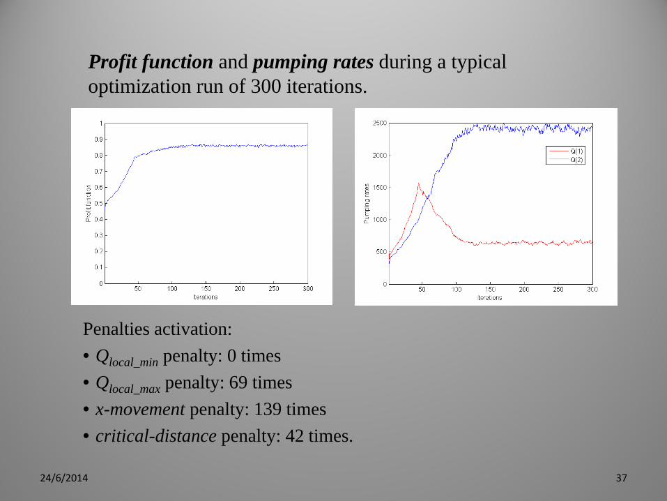
Profit function and pumping rates during a typical optimization run of 300 iterations.

Penalties activation: • Qlocal_min penalty: 0 times • Qlocal_max penalty: 69 times • x-movement penalty: 139 times • critical-distance penalty: 42 times.

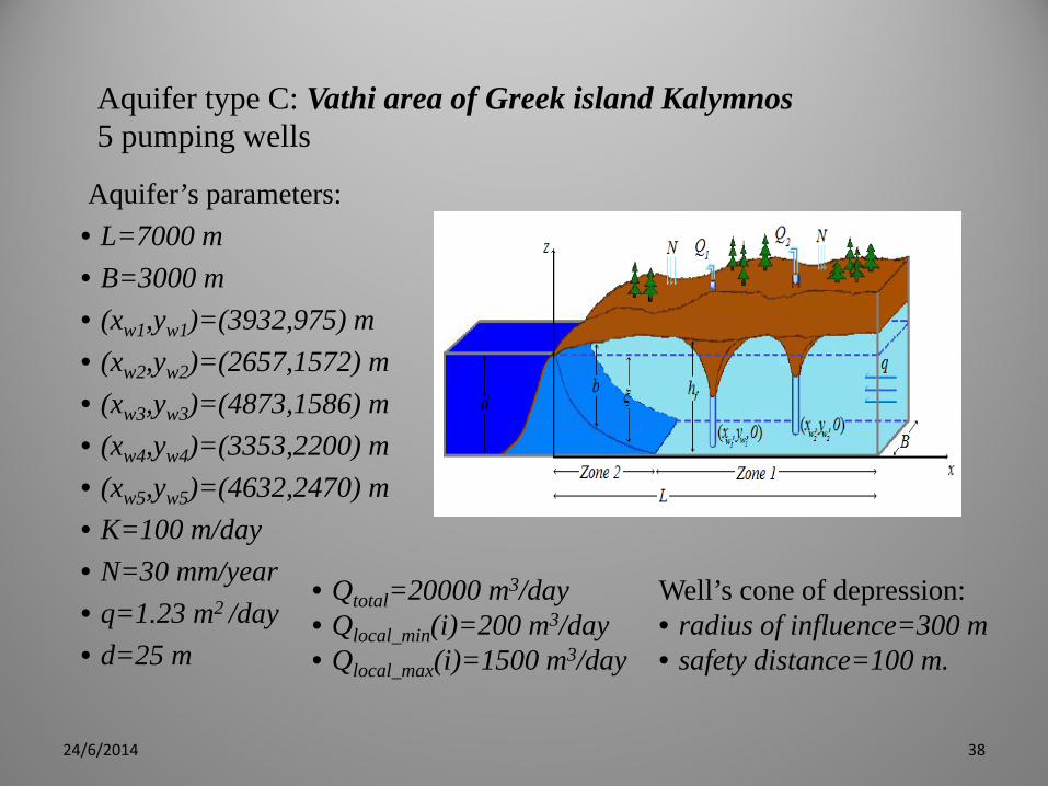
Aquifer type C: Vathi area of Greek island Kalymnos 5 pumping wells

Aquifer’s parameters: • L=7000 m • B=3000 m • (xw1,yw1)=(3932,975) m • (xw2,yw2)=(2657,1572) m • (xw3,yw3)=(4873,1586) m • (xw4,yw4)=(3353,2200) m • (xw5,yw5)=(4632,2470) m • K=100 m/day • N=30 mm/year • q=1.23 m2 /day • d=25 m

38 24/6/2014

Well’s cone of depression: • radius of influence=300 m • safety distance=100 m.

• Qtotal=20000 m3/day • Qlocal_min(i)=200 m3/day • Qlocal_max(i)=1500 m3/day

Algorithm parameters: • c=0.6: acceleration factor • noise(i)(k)=0.05*Q(i)(k)*rand.

24/6/2014 39

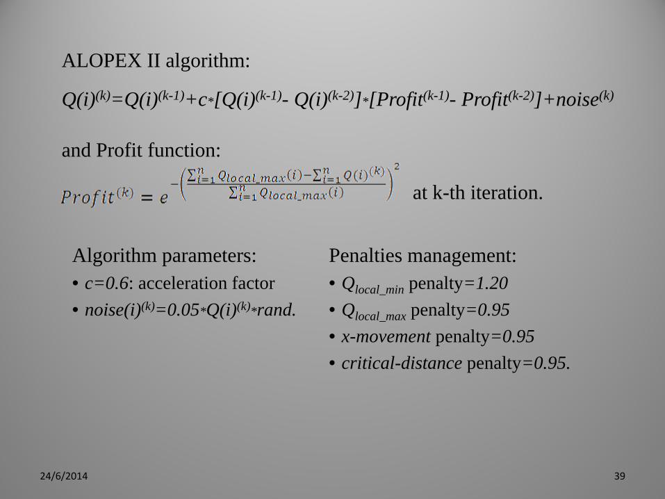
ALOPEX II algorithm:

and Profit function:

at k-th iteration.

Penalties management: • Qlocal_min penalty=1.20 • Qlocal_max penalty=0.95 • x-movement penalty=0.95 • critical-distance penalty=0.95.

Q(i)(k)=Q(i)(k-1)+c*[Q(i)(k-1)- Q(i)(k-2)]*[Profit(k-1)- Profit(k-2)]+noise(k)

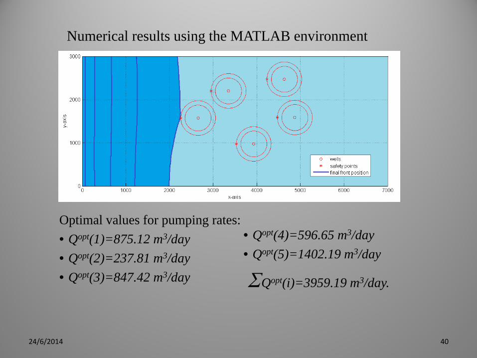
Numerical results using the MATLAB environment

24/6/2014 40

Optimal values for pumping rates: • Qopt(1)=875.12 m3/day • Qopt(2)=237.81 m3/day • Qopt(3)=847.42 m3/day

• Qopt(4)=596.65 m3/day • Qopt(5)=1402.19 m3/day

ΣQopt(i)=3959.19 m3/day.

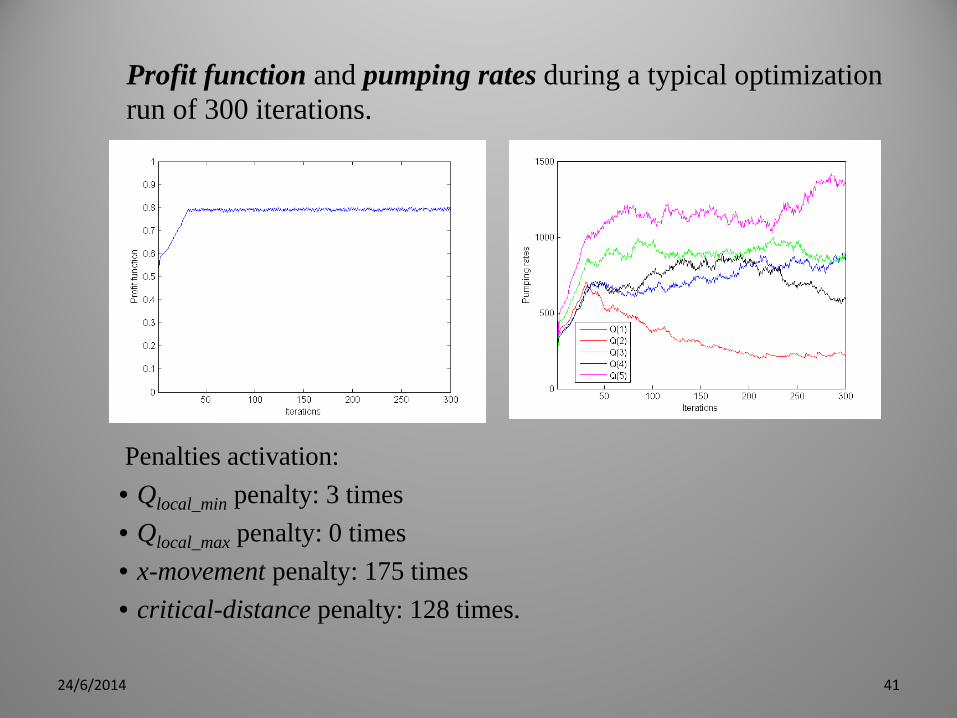
Profit function and pumping rates during a typical optimization run of 300 iterations.

24/6/2014 41

Penalties activation: • Qlocal_min penalty: 3 times • Qlocal_max penalty: 0 times • x-movement penalty: 175 times • critical-distance penalty: 128 times.

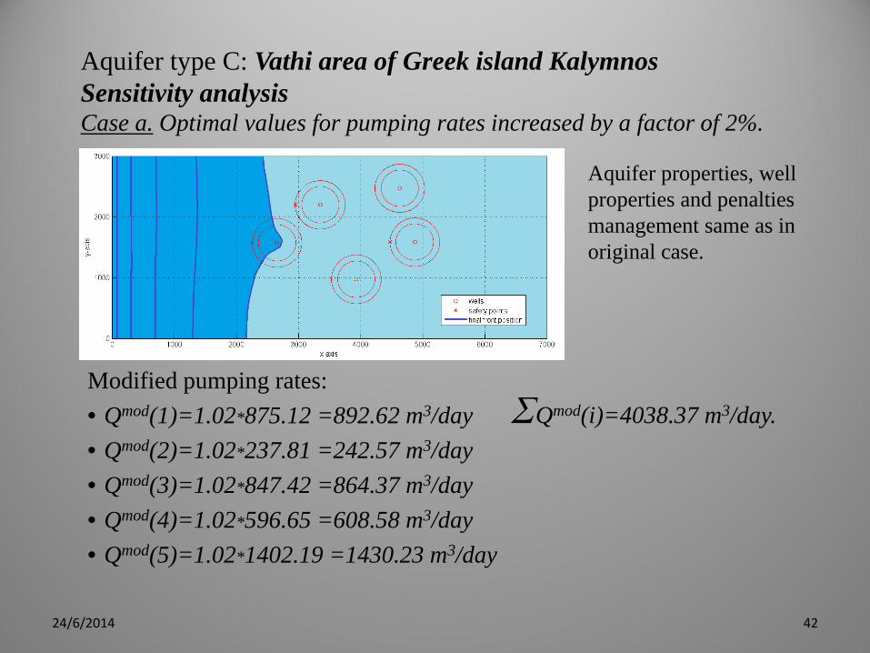
Aquifer type C: Vathi area of Greek island Kalymnos Sensitivity analysis Case a. Optimal values for pumping rates increased by a factor of 2%.

Modified pumping rates: • Qmod(1)=1.02*875.12 =892.62 m3/day • Qmod(2)=1.02*237.81 =242.57 m3/day • Qmod(3)=1.02*847.42 =864.37 m3/day • Qmod(4)=1.02*596.65 =608.58 m3/day • Qmod(5)=1.02*1402.19 =1430.23 m3/day

24/6/2014 42

ΣQmod(i)=4038.37 m3/day.

Aquifer properties, well properties and penalties management same as in original case.

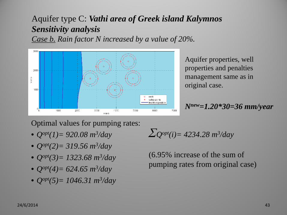
Aquifer type C: Vathi area of Greek island Kalymnos Sensitivity analysis Case b. Rain factor N increased by a value of 20%.

24/6/2014 43

Optimal values for pumping rates: • Qopt(1)= 920.08 m3/day • Qopt(2)= 319.56 m3/day • Qopt(3)= 1323.68 m3/day • Qopt(4)= 624.65 m3/day • Qopt(5)= 1046.31 m3/day

Aquifer properties, well properties and penalties management same as in original case. Nnew=1.20*30=36 mm/year

ΣQopt(i)= 4234.28 m3/day (6.95% increase of the sum of pumping rates from original case)

24/6/2014 44

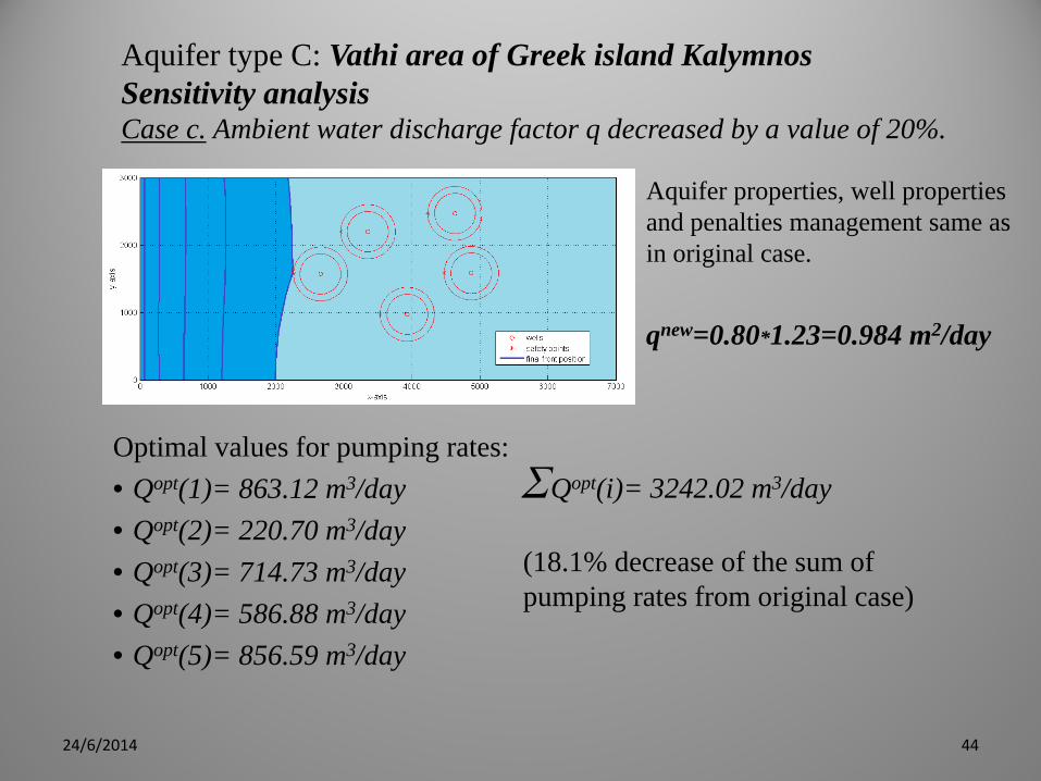
Aquifer type C: Vathi area of Greek island Kalymnos Sensitivity analysis Case c. Ambient water discharge factor q decreased by a value of 20%.

Aquifer properties, well properties and penalties management same as in original case. qnew=0.80*1.23=0.984 m2/day

Optimal values for pumping rates: • Qopt(1)= 863.12 m3/day • Qopt(2)= 220.70 m3/day • Qopt(3)= 714.73 m3/day • Qopt(4)= 586.88 m3/day • Qopt(5)= 856.59 m3/day

ΣQopt(i)= 3242.02 m3/day (18.1% decrease of the sum of pumping rates from original case)

24/6/2014

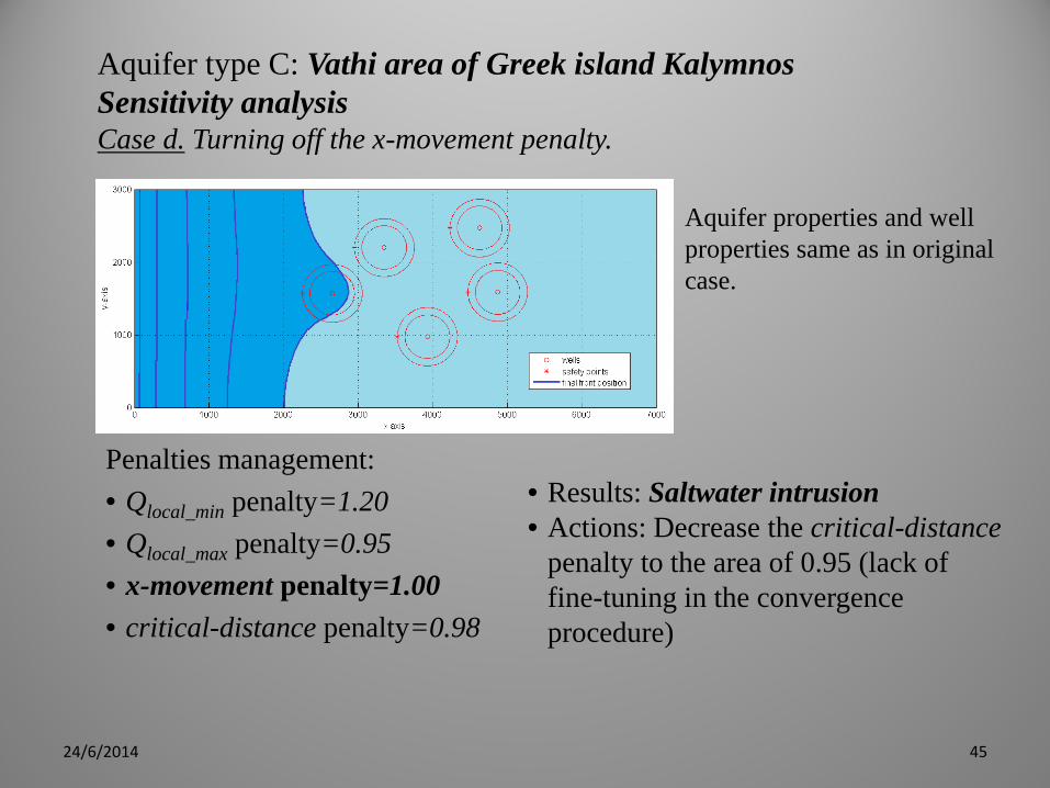
Aquifer type C: Vathi area of Greek island Kalymnos Sensitivity analysis Case d. Turning off the x-movement penalty.

Aquifer properties and well properties same as in original case.

Penalties management: • Qlocal_min penalty=1.20 • Qlocal_max penalty=0.95 • x-movement penalty=1.00 • critical-distance penalty=0.98

45

• Results: Saltwater intrusion • Actions: Decrease the critical-distance

penalty to the area of 0.95 (lack of fine-tuning in the convergence procedure)

24/6/2014 46

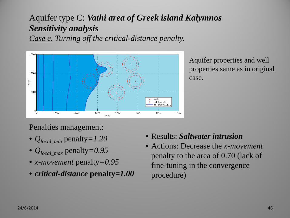
Aquifer type C: Vathi area of Greek island Kalymnos Sensitivity analysis Case e. Turning off the critical-distance penalty.

Aquifer properties and well properties same as in original case.

Penalties management: • Qlocal_min penalty=1.20 • Qlocal_max penalty=0.95 • x-movement penalty=0.95 • critical-distance penalty=1.00

• Results: Saltwater intrusion • Actions: Decrease the x-movement

penalty to the area of 0.70 (lack of fine-tuning in the convergence procedure)

Discussion and conclusions • The present work implements the ALOPEX optimization method to

the problem of prevention of salinization in freshwater aquifers.

• The study is based on a well known model of freshwater aquifers and its analytical solution for the water flow potential. The ALOPEX method is chosen to calculate the optimal pumping rates of the aquifer wells, due to the advantages of the method when compared to other optimization tools.

• Simulations are presented for i) a hypothetical case of an aquifer with two wells and ii) the real aquifer case of Vathi (on the island of Kalymnos, Greece). A study on the sensitivity of the optimization process on the case of the aquifer of Vathi has also been performed, confirming the efficiency and applicability of the optimization method, as well as the need of the penalties imposed.

24/6/2014 47

A few words about the advantages of ALOPEX optimization method.

• by incorporating stochasticity, the method effectively finds the global maxima or minima without local convergence yet in a manner that does not require inefficient scanning for the solution.

• the profit function of the method is a scalar that measures global performance and can thus contain a large number of variables (related to the pumping rates of the aquifer wells), which may be simultaneously adjusted.

• the same optimization process can be applied in real time and is thus able to control the volume of pumping water in a real aquifer environment.

24/6/2014 48

24/6/2014 49

• The method can be applied together with different pumping policies for the aquifer areas, giving us full control of the pumping management.

For example, minimum and maximum pumping rates can differ for every well in controlling the volume of water distributed over the area. In this way, areas with different water needs (cities or agricultural areas) can be provided with no-less than the volume of water they actually need.

• No knowledge of the dynamics of the system or of the functional dependence of the cost function on the control variables, is required, making this way the method applicable to further, more realistic simulations where no analytical solutions are provided.

References • [CHNO]A.H.-D. Cheng, D. Halhal, A. Naji and D. Ouazar, Pumping

optimization in salt water-intruded coastal aquifers, Water Resour. Res., Vol. 36, No.8, pp.2155-2165, 2000.

• [HT]E. Harth, E. Tzanakou, Alopex: A stochastic method for determining visual receptive fields, Vision Research, 14, pp.14751482, 1974.

• [K1]K.L. Katsifarakis, Groundwater pumping cost minimization – an analytical approach, Water Resources Management, vol.22, No 8, pp.1089-1099, 2007.

• [KSZ]T. Kalogeropoulos, Y. Saridakis, M. Zakynthinaki, Improved stochastic optimization algorithms for adaptive optics, Comp. Phys. Commun. 99, 255, 1997.

• [M1]A. Mantoglou, A theoretical approach for modeling unsaturated flow in spatially variable soils: Effective flow models in finite domains and nonstationarity, Water Resources Research, 28, No.1, pp.251-257, 1992.

• [M2]A. Mantoglou, Pumping management of coastal aquifers using analytical models of salt water intrusion, Water Recourses Research, ISSN 0043-397, 39(12), 2003.

50 24/6/2014

24/6/2014 51

• [MPG]A. Mantoglou , M. Papantoniou and P. Giannoulopoulos, Management of coastal aquifers based on nonlinear optimization and evolutionary algorithms, J. Hydrol., 297, pp.209-228, 2004.

• [MMT]L. Melissaratos, E. Micheli-Tzanakou, A parallel implementation of the ALOPEX process., J. Med. Syst. 13 (5) (1989) 243.

• [MT1]E. Micheli-Tzanakou, Supervised and Unsupervised Pattern Recognition: Feature Extraction and Computational Intelligence, Boca Raton, FL: CRC Press, 2000.

• [PV]A.S. Pandya, K.P. Venugopal, A stochastic parallel algorithm for supervised learning in neural networks, IEICE Trans. Inform. Syst. E77-D (4) (1994) 376-384.

• [PSH]A.S. Pandya, E. Sen, S. Hsu, Buffer allocation optimization in ATM switching networks using ALOPEX algorithm, Neurocomput. 24 (1–3) (1999) 1-11.

• [SANPK]H. Shintani, M. Akutagawa, H. Nagashino, A. S. Pandya, Y. Kinouchi, Optimization of MLP/BP for character recognition using a modified alopex algorithm. KES 11(6): 371-379 (2007)

• [S1]O.D.L. Strack, Groundwater Mechanics, Prentice Hall, 1989.

24/6/2014 52

• [TMH]E. Tzanakou, R. Michalak, E. Harth, The ALOPEX process: Visual receptive fields by response feedback, Biol. Cybernet. 35 (1979) 161.

• [T1]D. K. Todd, Salt water intrusion of coastal aquifers in the United States, Subterranean Water, 52, pp.452–461, 2009.

• [UV]K.P. Unnikrishnan, K.P. Venugopal, Alopex: A correlation-based learning algorithm for feed-forward and recurrent neural networks, Neural Comput. 6 (3) (1994) 469-490.

• [ZBMM]M. Zakynthinaki, R.O. Barakat, C.A. Cordente Martínez, J. Sampedro Molinuevo, Stochastic optimization for the detection of changes in maternal heart rate kinetics during pregnancy, Comp. Phys. Commun. 182, 683–691, 2011.

• [ZS1]M. Zakynthinaki, Y. Saridakis, Stochastic optimization for a tip-tilt adaptive correcting system, Comp. Phys. Commun. 150 (3), 274, 2003.

• [ZS2]M. Zakynthinaki, J.R. Stirling, Stochastic optimization for modeling physiological time series: application to the heart rate response to exercise, Comp. Phys. Commun. 176 (20), 98, 2007.