Physics of the interac/ons between iner/al par/cles and ...

Physicsoftheinterac/onsbetweeniner/alpar/clesandturbulence

AlbertoAlisedaDepartmentofMechanicalEngineering

UniversityofWashington([email protected])

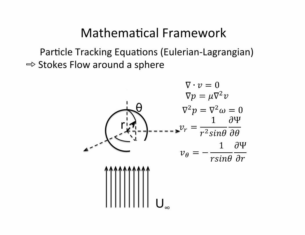
Mathema/calFrameworkPar/cleTrackingEqua/ons(Eulerian-Lagrangian)

➾ StokesFlowaroundasphere

θ

φ

r

U∞

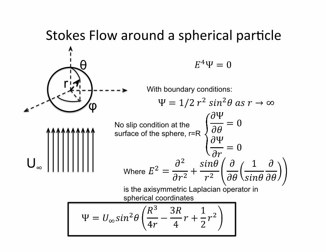
StokesFlowaroundasphericalpar/cle

θ

φ

r

U∞

With boundary conditions:

No slip condition at the surface of the sphere, r=R

Where is the axisymmetric Laplacian operator in spherical coordinates

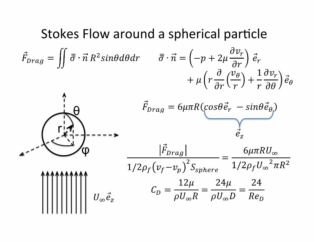
StokesFlowaroundasphericalpar/cle

θ

φ

r

!!!! !

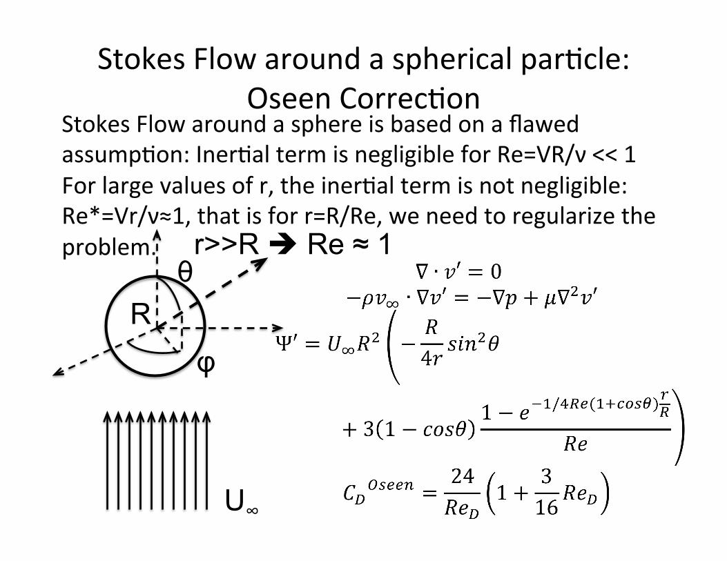
StokesFlowaroundasphericalpar/cle:OseenCorrec/on

StokesFlowaroundasphereisbasedonaflawedassump/on:Iner/altermisnegligibleforRe=VR/ν<<1Forlargevaluesofr,theiner/altermisnotnegligible:Re*=Vr/ν≈1,thatisforr=R/Re,weneedtoregularizetheproblem.

θ

φ

r>>R è Re ≈ 1

U∞

R

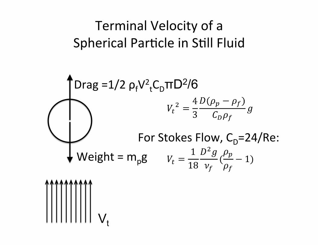
TerminalVelocityofaSphericalPar/cleinS/llFluid

Vt

Drag=1/2ρfV2tCDπD2/6

Weight=mpg

ForStokesFlow,CD=24/Re:

!! =118!!!!!

(!!!!− 1)!

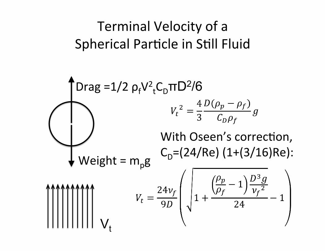
TerminalVelocityofaSphericalPar/cleinS/llFluid

Vt


Weight=mpg

WithOseen’scorrec/on,CD=(24/Re)(1+(3/16)Re):

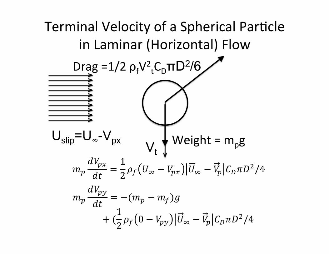
TerminalVelocityofaSphericalPar/cleinLaminar(Horizontal)Flow

Vt


Weight=mpgUslip=U∞-Vpx

!!!!!"!" = −(!! −!!)!

+ (12!! 0− !!" !! − !! !!!!!/4!

!! =118!!!!!

(!!!!− 1)!

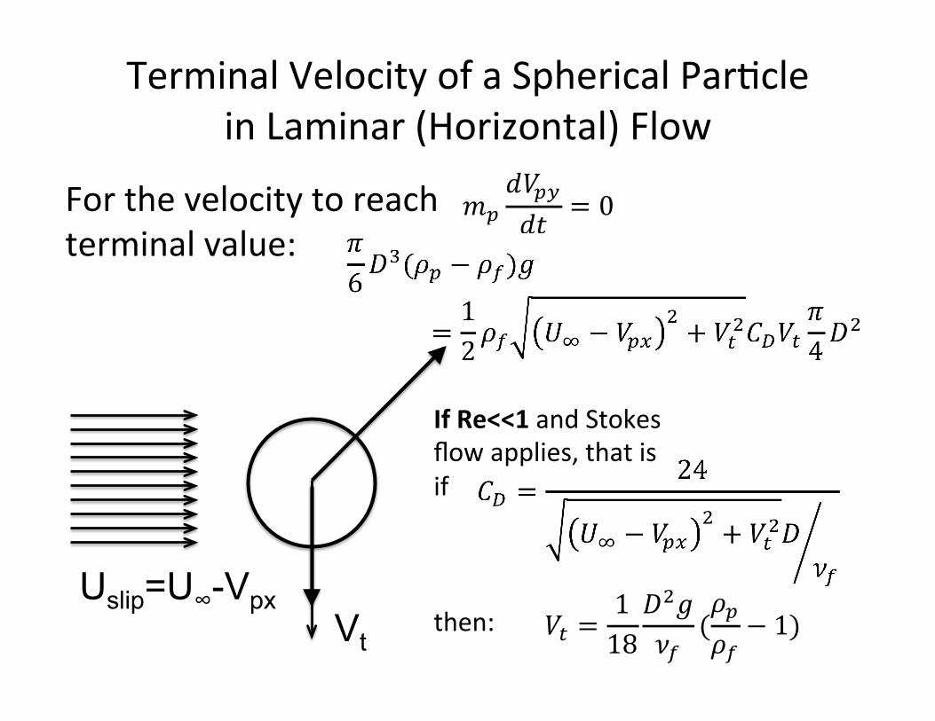
TerminalVelocityofaSphericalPar/cleinLaminar(Horizontal)Flow

Vt Uslip=U∞-Vpx

!!!!!"!" = 0!Forthevelocitytoreach

terminalvalue:

IfRe<<1andStokesflowapplies,thatisifthen:

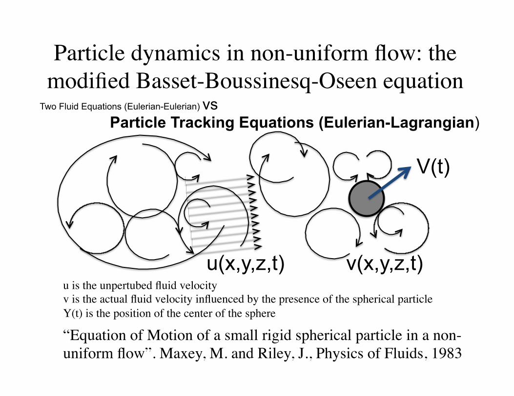
“Equation of Motion of a small rigid spherical particle in a non-uniform flow”. Maxey, M. and Riley, J., Physics of Fluids, 1983

Particle dynamics in non-uniform flow: the modified Basset-Boussinesq-Oseen equation

Two Fluid Equations (Eulerian-Eulerian) vs Particle Tracking Equations (Eulerian-Lagrangian)

u is the unpertubed fluid velocityv is the actual fluid velocity influenced by the presence of the spherical particleY(t) is the position of the center of the sphere

u(x,y,z,t)

V(t)

v(x,y,z,t)

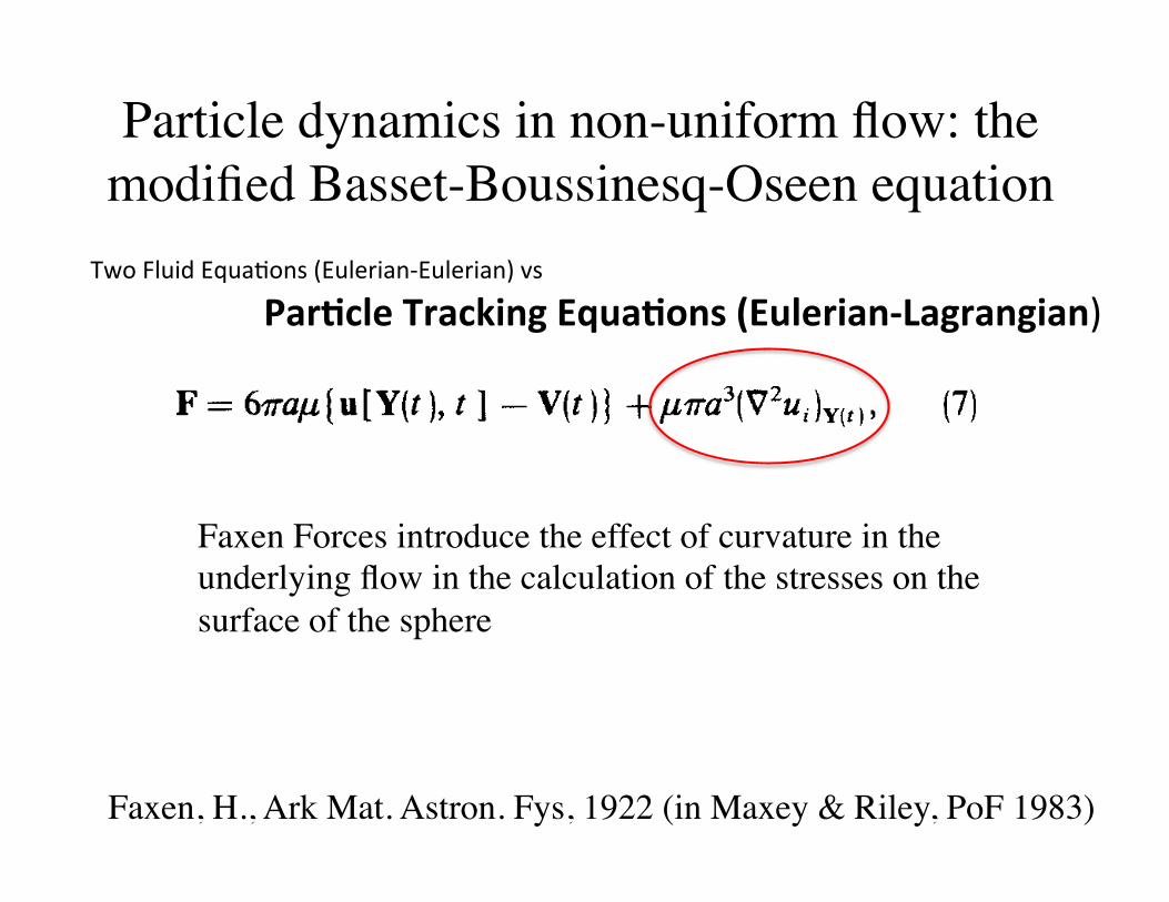
Faxen, H., Ark Mat. Astron. Fys, 1922 (in Maxey & Riley, PoF 1983)


TwoFluidEqua/ons(Eulerian-Eulerian)vsPar+cleTrackingEqua+ons(Eulerian-Lagrangian)

Downloaded 01 Oct 2007 to 128.95.34.46. Redistribution subject to AIP license or copyright, see http://pof.aip.org/pof/copyright.jsp

Faxen Forces introduce the effect of curvature in the underlying flow in the calculation of the stresses on the surface of the sphere


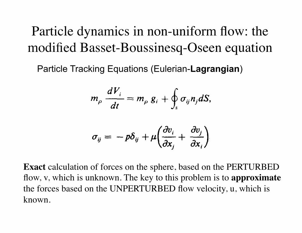
Particle Tracking Equations (Eulerian-Lagrangian)

Equations of motion for the fluids are expressed in an Eulerian Frame: Cons. of mass, cons. of Momentum, no slip velocity on the surface of the sphere, velocity of the fluid (v) is equal to the unperturbed velocity of the fluid as the distance to the particle tends to infinity



Exact calculation of forces on the sphere, based on the PERTURBED flow, v, which is unknown. The key to this problem is to approximate the forces based on the UNPERTURBED flow velocity, u, which is known.


Particle Tracking Equations (Eulerian-Lagrangian)



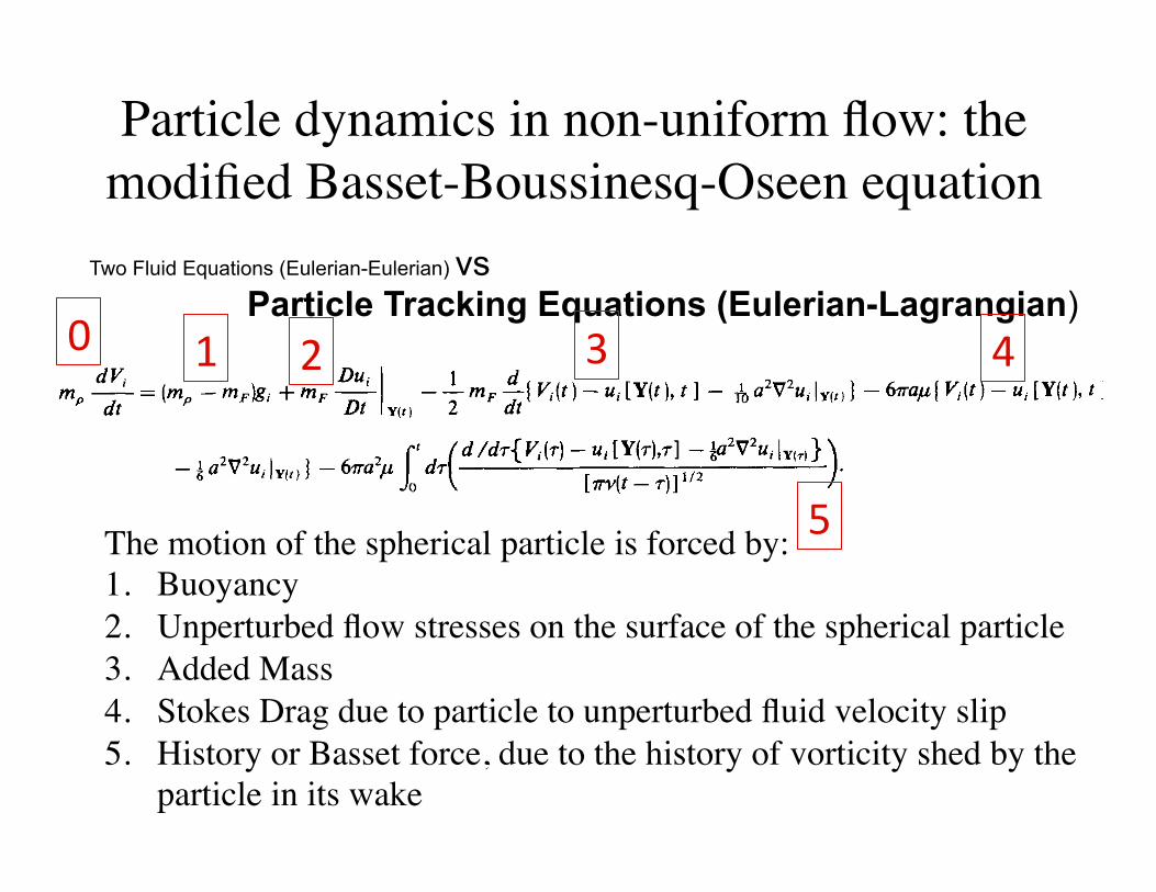
Two Fluid Equations (Eulerian-Eulerian) vs Particle Tracking Equations (Eulerian-Lagrangian)

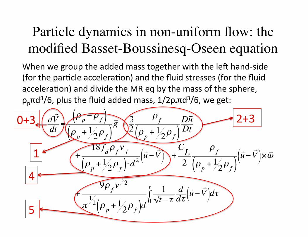
The motion of the spherical particle is forced by:1.  Buoyancy2.  Unperturbed flow stresses on the surface of the spherical particle3.  Added Mass4.  Stokes Drag due to particle to unperturbed fluid velocity slip5.  History or Basset force, due to the history of vorticity shed by the

particle in its wake


1 2 3 4

5

0

€

d V

dt =ρ p −ρ f( )ρ p + 1

2ρ f( ) g + 3

2ρ f

ρ p + 12ρ f( )

D u Dt

+18 fdρ fν f

ρ p + 12ρ f( )⋅d2

u −

V & ' (

) * + +

CL2

ρ f

ρ p + 12ρ f( )

u − V &

' (

) * + × ω

+9ρ fν

12

π1

2 ρ p + 12ρ f( )d

1t−τ

ddτ u −

V & ' (

) * + dτ

0

t∫

Whenwegrouptheaddedmasstogetherwiththeledhand-side(forthepar/cleaccelera/on)andthefluidstresses(forthefluidaccelera/on)anddividetheMReqbythemassofthesphere,ρpπd3/6,plusthefluidaddedmass,1/2ρfπd3/6,weget:


0+3

4

5

2+3

1

A note about the scales of turbulence

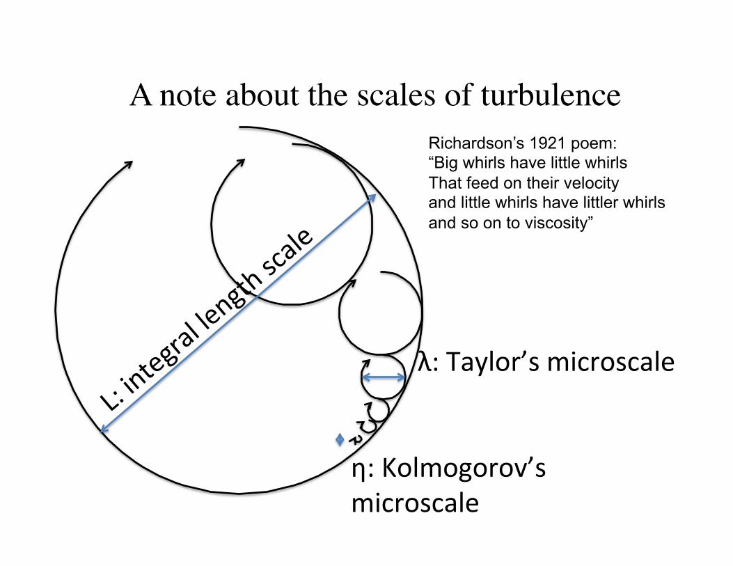
λ:Taylor’smicroscale

η:Kolmogorov’smicroscale

Richardson’s 1921 poem: “Big whirls have little whirls That feed on their velocity and little whirls have littler whirls and so on to viscosity”

48

0

0 0

V 0 0 - b 0

V m 0 D -

O 8 - 0

0

I I

103

10'

10'

E(K)I1 Eo

1 OD

lo-'

lo-? C

M . R. Wells and D . E . Stock

; 1

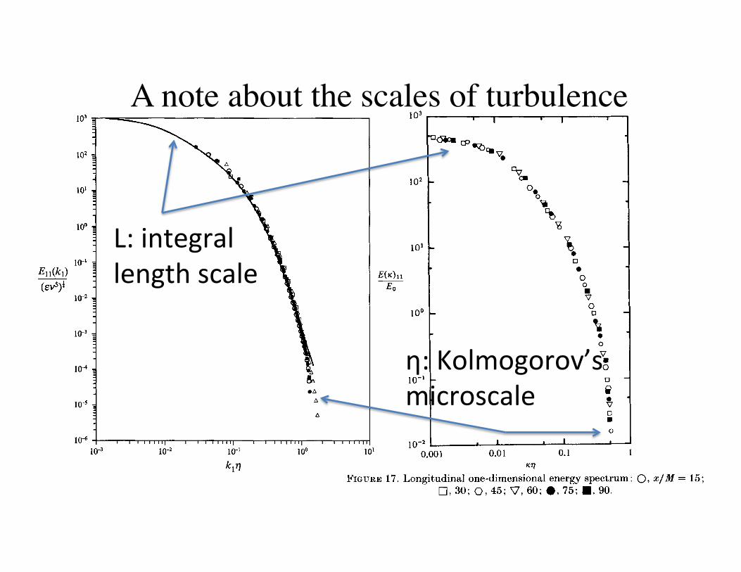
FIGURE 17. Longitudinal one-dimensional energy spectrum : 0, x / M = 15; 0, 30; 0 , 45; V, 60; 0 , 75; H, 90.

The longitudinal and lateral power spectra plotted in Kolmogoroff coordinates are shown in figures 17 and 18 respectively. The coordinates are non-dimensionalized using Eo = (eV5)k, k = 27cf/u and 7 = ($/€)a, where e and f are the turbulent eddy dissipation and frequency respectively. In the region of high wavenumber the spectral profiles were found to collapse to a single curve.

A check of the spectral estimates was made by comparing the results of two methods of calculating the eddy dissipation per unit mass. First assuming homogeneous turbulence and a constant mean velocity, the turbulent kinetic-energy equation reduces to (Hinze 1959, p. 75)

dq2 2 dt _- - - -€,

then making the transformation d - - d -- - u- dt dx

gives odp 2 dx €=- - - -

By assuming q2 = 3,d2, where pf2 = ur2 = d2 = wT2, e may be calculated by fitting q2 versus x- xo and differentiating. The dissipation may also be calculated directly from the measured spectral-energy function (Hinze 1959)

r m

Settling velocity and concentration distribution of particles 35 103

102

10'

100

lo-'

10-3

1 0-4

A

A

I I I I I I l l 1 I I I I I I l l 1 I I I I I I l l 1 I I I I I I T

10-3 10-2 lo-' loo 10'

417 FIGURE 2. The one-dimensional energy spectra for the simulated flows at various Re, under Kolmogorov scaling: 0, 323, Re, = 21; ., 483, Re, = 31; 0, 643, Re, = 43; e, 963, Re, = 62; A, 483 and use of the second forcing scheme, Re, = 30. The line is a curvefit for all the measured data taken from Comte-Bellot & Corrsin (1971) for a flow behind a 2-in grid.

Wells & Stock (1983), both of which studied the dispersion of heavy particles in a grid- generated turbulence, and found that all the experimental curves agree very well for ky 2 0.01. Such universality of the energy spectrum is reproduced by the simulations, although this is somewhat surprising as the flow Reynolds numbers are not high. The flow Reynolds numbers for all the above experimental measurements are comparable to those in our simulations. As a side note, George (1992) recently suggested a different scaling using h and u' for the energy spectrum rather than Kolmogorov scaling for self- preserving decaying turbulence. For our forced stationary turbulence, we found, however, the Kolmogorov scaling collapses data much better than the suggested Taylor scaling.

Finally, the velocity derivative skewness and flatness are shown in table 1. The velocity derivative skewness in our simulations is in the range -0.55 to -0.40, which compares very well with the experimental range -0.5 to - 0.3 for Re, < 100 (Van Atta & Antonia 1980). The flatness also agrees with the experimental value of about 4. In summary, although the simulated flows are contaminated by the artificial forcing and

A note about the scales of turbulence

L:integrallengthscale

η:Kolmogorov’smicroscale

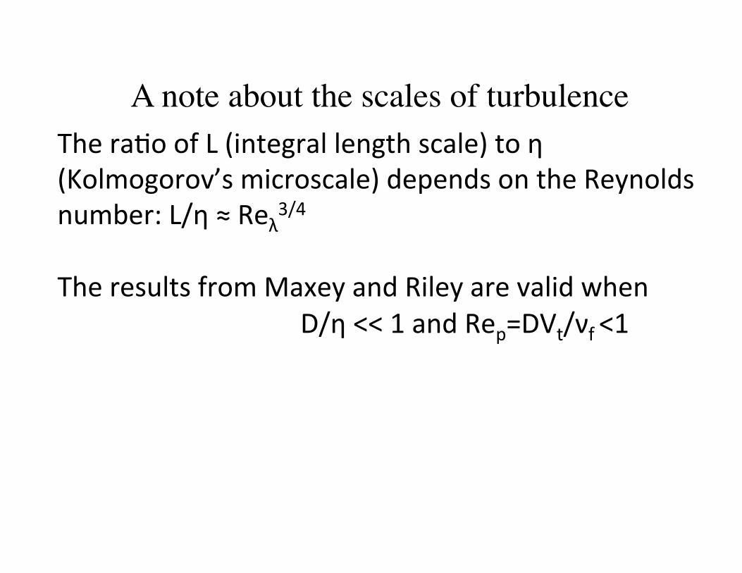
A note about the scales of turbulenceThera/oofL(integrallengthscale)toη(Kolmogorov’smicroscale)dependsontheReynoldsnumber:L/η≈Reλ3/4TheresultsfromMaxeyandRileyarevalidwhen D/η<<1andRep=DVt/νf<1

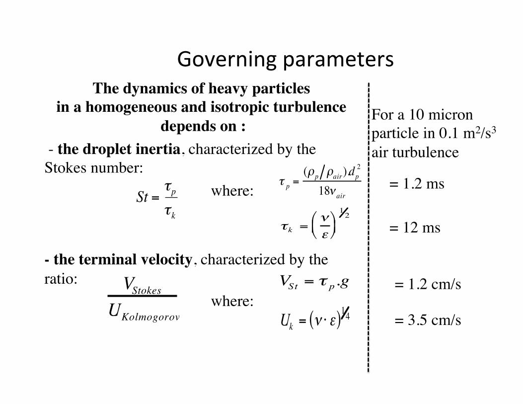
The dynamics of heavy particles �in a homogeneous and isotropic turbulence�

depends on : - the droplet inertia, characterized by the Stokes number: where:

- the terminal velocity, characterized by the ratio: where:

VStokesUKolmogorov

VSt = τ p.g€

St =τpτk

τ p =(ρp ρair).dp

2

18ν air

τk =νε

$ % & ' ( ) 12

Uk = ν ⋅ ε( )14

Governingparameters

= 1.2 ms

= 12 ms

= 1.2 cm/s

= 3.5 cm/s

For a 10 micron particle in 0.1 m2/s3 air turbulence

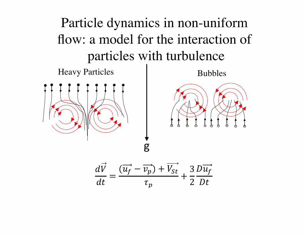
Heavy Particles Bubbles

Particle dynamics in non-uniform flow: a model for the interaction of

particles with turbulence

g

€

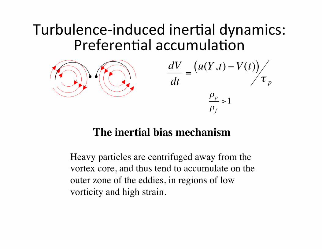
dVdt

=u(Y ,t) −V (t)( )

τ p

€

ρ p

ρ f>1

Heavy particles are centrifuged away from the vortex core, and thus tend to accumulate on the outer zone of the eddies, in regions of low vorticity and high strain.

The inertial bias mechanism

Turbulence-inducediner/aldynamics:Preferen/alaccumula/on

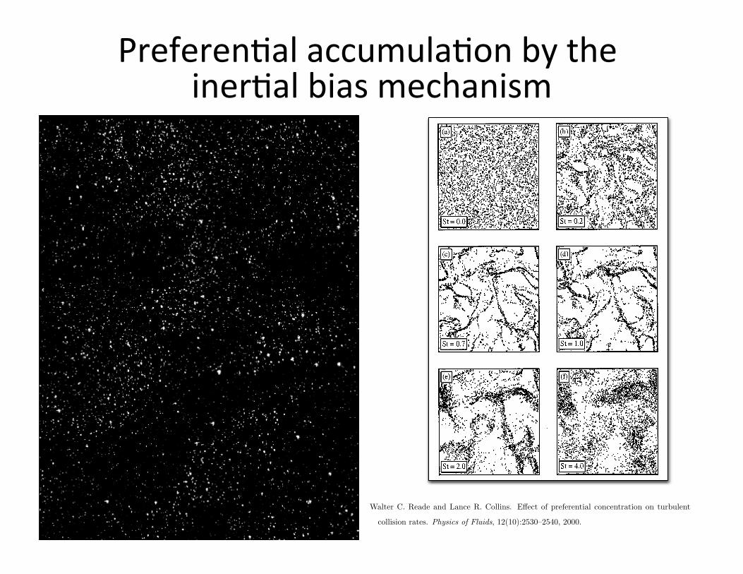
Preferen/alaccumula/onbytheiner/albiasmechanism

1!c"# suggests that the regions with little or no particles areon the order of 1/10 the box length, making the size of these

regions on the order of 10$.

III. MODELING CONSIDERATIONS

A. Radial distribution function

Consider a canonical ensemble of systems, each of vol-

ume V , containing N indistinguishable particles of diameter,

%, and density, &p . For such an ensemble, the joint probabil-ity that each of the N particles lie within volumes dx1 cen-

tered at x1 ,. . . , through dxN centered at xN is defined as

P !N "!x1 ,. . . ,xN"dx1 .. .dxN , !7"

where the standard normalization applies, i.e.,

!V

¯!V

P !N "!x1 ,. . . ,xN"dx1¯dxN!1. !8"

The two-particle distribution function is then obtained by

integrating out the dependence on the remaining particles

P !2 "!x1 ,x2"'!V

¯!V

P !N "!x1 ,. . . ,xN"dx3¯dxN . !9"

The two-particle radial distribution function is then defined

as32,33

g!x1 ,x2"!N!N"1 "

n2P !2 "!x1 ,x2", !10"

where n'N/V . For a statistically homogeneous and isotro-

pic volume, particle positions can be expressed in terms of a

relative separation distance, r'"x1"x2", and P (2)(x1 ,x2) re-duces to P (2)(r)/V to give the working definition of g(r)

used in this study

g!r "!N!N"1 "

n2VP !2 "!r ". !11"

As the rdf is near unity for a uniformly distributed system, it

is convenient to define a residual rdf !rrdf" as

h!r "'g!r ""1. !12"

A physical interpretation of g(r) is the number of par-

ticle centers located in a spherical shell between r and r

#dr about a central particle divided by the expected number

of particles given a uniformly distributed particle field.

Based on the definition of the rdf shown in Eq. !11" and theintegral relationship given in Eq. !8", it is easy to show thatthe rrdf must satisfy the following integral constraint34

n!V

h!r "dr!"1. !13"

B. Parametric dependence

Isotropic turbulence is characterized by the fluid density,

&, kinematic viscosity, v , turbulence intensity U!, and ki-netic energy dissipation rate, (. In dimensionless terms, thisreduces to the turbulent Reynolds number, defined here in

terms of the Taylor microscale

Re)'U!2!15

v(. !14"

For a monodisperse suspension, the particle phase introduces

three additional variables, viz., the particle density &p , diam-eter %, and total number N. In terms of dimensionless vari-ables, these can be expressed as the volumetric loading *'+%3N/6V , nondimensional size parameter %̂'%/$ and

particle Stokes number St ,see Eq. !1"#. This implies that themost general form of the rdf in isotropic turbulence can be

expressed functionally as

g! r̂;Re) ,* ,%̂ ,St", !15"

where r̂'r/$ is the dimensionless independent variable and

the variables after the semicolon are the dimensionless pa-

rameters.

C. Simplifying assumptions

The large parameter space shown in Eq. !15" wouldmake it difficult to interpret and correlate the results from the

numerical simulations. It is, therefore, advantageous to con-

sider the sensitivity of the rdf to each of the parameters, and

search for simplifications where applicable.

FIG. 1. 2d slices of ghost-particle simulations at: !a" St!0.0; !b" St!0.2;!c" St!0.7; !d" St!1.0; !e" St!2.0; and, !f" St!4.0. Dots correspond toparticle center locations.

2533Phys. Fluids, Vol. 12, No. 10, October 2000 Effect of preferential concentration on turbulent collision rates

Downloaded 21 Mar 2010 to 128.95.104.66. Redistribution subject to AIP license or copyright; see http://pof.aip.org/pof/copyright.jsp

75

M.R. Maxey. The motion of small spherical particles in a cellular flow field. Phys. Fluids,

30(4):1915–1928, 1987a.

M.R. Maxey. The gravitational settling of aerosol particles in homogeneous turbulence and

random flow fields. J. Fluid Mech., 174:441–465, 1987b.

M.R. Maxey and S. Corrsin. Gravitational settling of aerosol particles in randomly oriented

cellular flows. J. Atmospher. Sci., 43:1112–1134, 1986.

M.R. Maxey and J.J. Riley. Equation of motion for a small rigid sphere in a nonuniform

flow. Phys. Fluids, 26(4):883–889, 1983.

M. S. Mohamed and J. C. LaRue. The decay power law in grid-generated turbulence. J.

Fluid Mech., 219:195–214, 1990.

M.B. Pinsky and A.P. Khain. Turbulence e�ects on the collision kernel. I: Formation of

velocity deviations of drops falling within a turbulent three-dimensional flow. Q. J. R.

Meteorol. Soc., 123:1517–1542, 1997.

M.B. Pinsky, A.P. Khain, and M. Shapiro. Turbulence e�ects on droplet growth and size

distribution in clouds - A review. J. Aerosol Sci., 28:1177–1214, 1997.

M.B. Pinsky, A.P. Khain, and M. Shapiro. Collisions of small drops in a turbulent flow.

Part I: Collision e⇥ciency. problem formulation and preliminary results. J. Atmospher.

Sci., 56(15):2585–2600, 1999.

M.B. Pinsky, A.P. Khain, and M. Shapiro. Stochastic e�ects of cloud droplet hydrodynamic

interaction in a turbulent flow. 53(1-3):131–169, 2000.

M.B. Pinsky, M. Shapiro, and A.P. Khain. Collision e⇥ciency of drops in a wide range of

Reynolds numbers: E�ect of pressure on spectrum evolution. J. Atmospher. Sci., 58(17):

742–764, 2001.

S.B. Pope. Turbulent Flows. Cambridge University Press, Cambridge, 2006.

Walter C. Reade and Lance R. Collins. E�ect of preferential concentration on turbulent

collision rates. Physics of Fluids, 12(10):2530–2540, 2000.

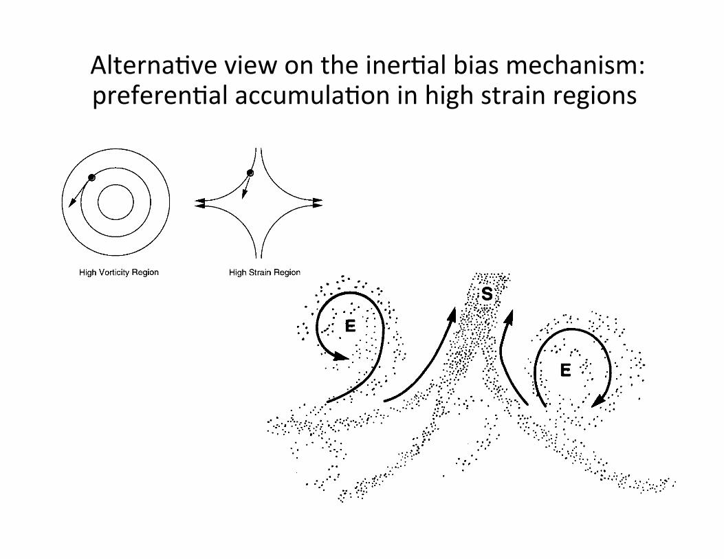
Alterna/veviewontheiner/albiasmechanism:preferen/alaccumula/oninhighstrainregions

Eddies, stream^, and Convergence Zones 203

FIGURE 1 ~ . or E zones for slow reactions.

Showing how reacting species (A,B) tend to react in C zones for fast

FIGURE 1B. Showing how particles tend to concentrate in the streaming S zones.

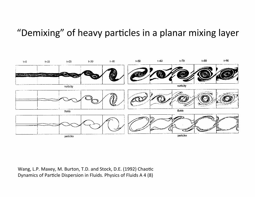
“Demixing”ofheavypar/clesinaplanarmixinglayer

Wang,L.P.Maxey,M.Burton,T.D.andStock,D.E.(1992)Chao/cDynamicsofPar/cleDispersioninFluids.PhysicsofFluidsA4(8)

vonicity VOtTkiV

fluids

I I I , I / i-‘--i

particles

Fc-ssqj 2 $ 7

/d / i,7&-” I

FIG. 21. Evolution of vorticity distribution for the shear layer and material lines for fluids and heavy particles.

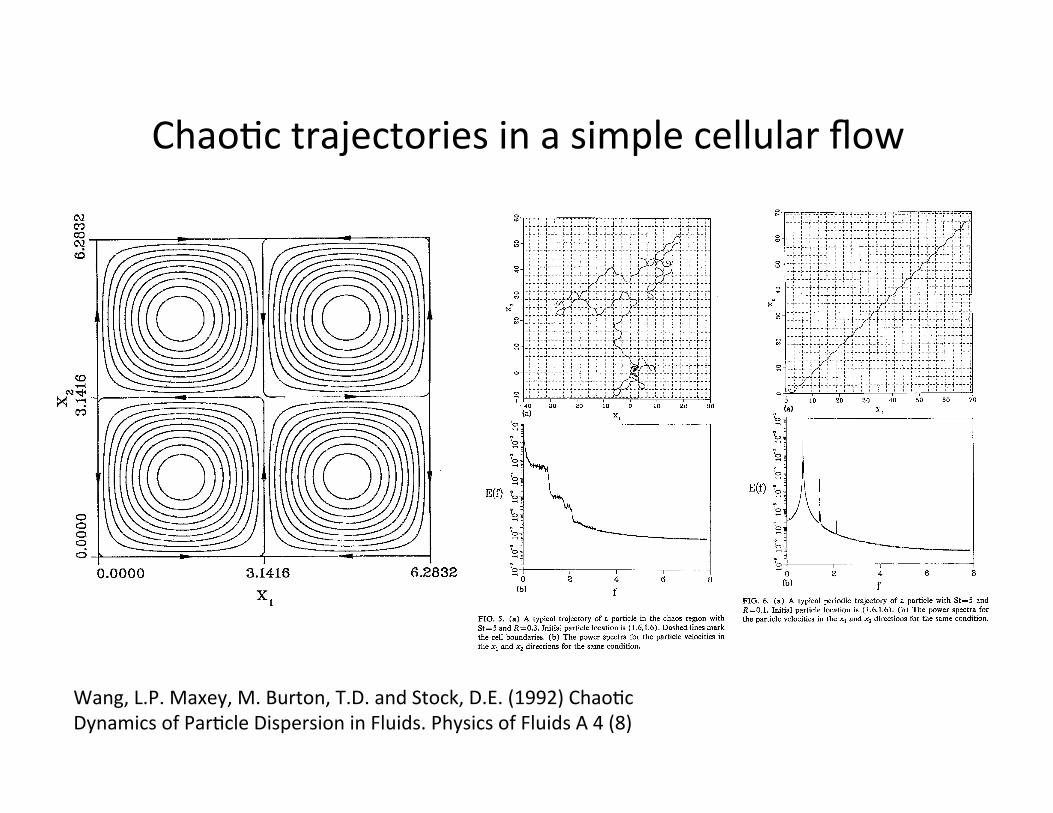
Chao/ctrajectoriesinasimplecellularflow

Wang,L.P.Maxey,M.Burton,T.D.andStock,D.E.(1992)Chao/cDynamicsofPar/cleDispersioninFluids.PhysicsofFluidsA4(8)

-40 -30 -20 -10 0 10 20 30 _ (a) Xl 7

b M t? ‘0 3-t

b

E(f) 7;

: 2

b e

“0 .+ P ;il 0 ii 4; 6 ;I

(b) f

FIG. 5. (a) A typica trajectory of a particle in the chaos region with St=5 and R=0.3. Initial particle location is (1.6,1.6). Dashed lines mark the cell boundaries. (b) The power spectra for the particle velocities in the x, and x2 directions for the same condition.

almost all the points have a positive average exponential growth rate. We expect that all the points will have a similar, single asymptotic growth rate when t-t CO, indicating that the long-term behavior is unique and independent of the initial location. Further evidence is presented later when the ergodicity of the system is discussed.

and u2 spectrum as expected. The broadband frequency contribution indicates the motion is chaotic. The power spectrum was obtained by taking a long time series of particle velocity (with 2048X50 data points) at a sampling rate of 2.5 samples per time unit. The VFFTPK library on Cray-YMP at the Pittsburgh Supercomputing Center (PSC) was used to derive the Fourier coefficients.

A typical trajectory for the chaotic motion is shown in Figure 6 shows a typical particle trajectory when the Fig. 5. The parameters used in this calculation are shown motion is periodic. It will be referred to as case II and the in Fig. 3 as point I. This set of parameters will be referred parameters are shown as point II in the parameter space of to as case I in later discussions. The initial particle location Fig. 3. In this case the particle travels along a 45” zigzag ( 1.6,1.6) is near the center of the cell. The particle moves curve. The power spectrum has a strong peak at the fun- along an outward spiral curve for some initial time due to damental frequency and its harmonics. The period is about inertial (centrifugal) force. The long-time motion is very 8.64 time units. In contrast with the periodic motion of irregular. The centrifugal effect does not allow the particle fluid elements where the orbit is closed streamlines, the to stay in any cell for long. Actually the particle seldom periodic motion of the aerosol particles follows an open visits the center of the cell where the vorticity is strong. At trajectory. In other words, the particle inertia destroys times the particle cuts through the cell boundary and en- closed periodic orbits and in turn can generate open peri- ters a new cell. This process repeats nonperiodically. Also odic orbits. It is noted that by open periodic orbits we do shown are the power spectra of the particle’s velocity at not distinguish (y, +2m7~, y,+2nr) from (y,, y2), where long time. There is no difference between the u1 spectrum m and n are arbitrary integers.

(a) by------- x1

5-5 2 4 6

lb) f FIG. 6. (a) A typical periodic trajectory of a particle with St=5 and R=O.l. Initial particle location is (1.6,1.6). (b) The power spectra for the particle velocities in the x1 and x2 directions for the same condition.

1793 Phys. Fluids A, Vol. 4, No. 8, August 1992 Wang et al. 1793

computed and the spatial complexity of the ABC flow, no relation between diffusivity and fractal dimension was found.

Some preliminary effort has been made to study La- grangian motion of particles in fully turbulent flows and shear mixing layers using dynamical systems tools. Wang et a1.9 used a finite number of random Fourier modes to represent unsteady, three-dimensional turbulent flow and computed the fractal dimension for the attractor of heavy particles. They found that the fractal dimension increased linearly with increasing particle diffusivity for a wide range of particle inertia and settling velocities. This suggests that the notion of chaos may be useful for studying particle dispersion and mixing in real turbulence. GaiZin-Calvo and Lasheras” used a steady Stuart vortex solution of the Eul- erian equations to represent a plane, free-shear layer and showed that heavy particles can be suspended in the layer and have periodic, quasiperiodic, or chaotic orbits. When the motion is chaotic, the attractor in physical space has a finite height, indicating some degree of transverse dispersion.

Most of the above studies are still of a preliminary nature. They raise many issues that need further, detailed investigation. Questions that come to mind include the following: Why does the appearance of chaos give rise to dispersion’? Does the occurrence of chaos guarantee dispersion? What measure based on chaotic dynamics is corre- lated to the dispersion coefficient? In this paper we address these issues by examining the Lagrangian motion of small, heavy particles in the steady two-dimensional cellular flow. Chaotic orbits are shown to exist and the resulting dispersion of particle clouds are found to have many of the fea- tures of turbulent dispersion. Correlations between the fractal dimension, the effective dispersion rate, and the effective mixing efficiency are explored. Finally particle dispersion and mixing in an evolving free-shear layer is briefly discussed in a similar context.

II. AEROSOL PARTICLES IN A CELLULAR FLOW

In this section we examine the Lagrangian motion of aerosol particles in a cellular flow. Such a flow arises in thermal convection with free-slip boundaries and has also been used to represent the transport effects of small-scale turbulent eddies on a passive scalar field.” Although the same flow was considered by C&anti et a1.,5 the equation of motion for particles adopted here is more general than in their work and a different particle parameter range is considered. Maxey and his co-workers, in a series of papers,W2,13 have studied the motion of small spherical and nonspherical particles in the same flow. Their main focus was on particle suspension and possible change in the particle mean settling rate. Our focus is on the chaotic motion of small spherical particles and the relationship between chaos, dispersion, and mixing.

A. Dynamical system

The steady, two-dimensional, and incompressible cellular flow is given in terms of streamfunction $ in fixed coordinates by

b.0000 3.i416 6.:

x1

FIG. 1. Streamlines in the cellular flow field. The increment in the values of streamfunction is 0.1.

4= sin x1 sin x2. (1) All the variables are assumed to be normalized by a char- acteristic length scale L and a velocity scale Ua of the flow.12 Typical streamlines are shown in Fig. 1. The flow extends with periodic repetition in both the x1 and x2 directions. The maximum flow velocity occurs on the cell boundaries, and there are stagnation points at the center of each cell and at the corners. The orbits for fluid elements are streamlines, thus the fluid motion for almost all initial conditions is periodic and regular with a period changing from 2~ near the center to infinity near cell boundaries. Equation ( 1) is a solution to the inviscid Euler equation for steady flow. The pressure is minimum at the center of the cell and maximum at the corners. The pressure gradient provides the force for the rotational motion of the fluid.

We restrict our study to small spherical particles in the aerosol range as defined by Maxey,12 that is, the ratio of the particle density to the fluid density is larger than 2, pdpf> 2. The particle equation of motion in a steady flow is given in a nondimensional form by12

dv u[Y(t),tl --v dt St +Ru*Vu+; RveVu. (2)

In these equations, v(t) and y(t) are particle velocity and location; u(x,t) is Eulerian flow velocity field, and, for the cellular flow, it is independent oft. The terms on the right- hand side of Eq. (2) represent Stokes drag, the pressure gradient force on the particle (more generally, the fluid force on an equivalent element from the undisturbed flow field), and the added mass effect. The effect of gravitational settling is not considered in the present paper. (One may assume that gravity is aligned in the direction normal to the two-dimensional plane and thus does not affect the motion in the plane.) Equation (2) is a simplified version


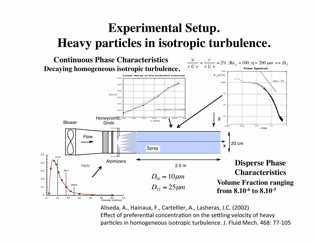
Experimental Setup. �Heavy particles in isotropic turbulence.

Volume Fraction ranging from 8.10-6 to 8.10-5

0

0.1

0.2

0.3

0.4

0.5

0 10 20 30 40 50 60 70

Pdf(D)

Diameter (microns)

St=1

SMD

D10

Disperse Phase Characteristics D10 ≈ 10µm

D32 ≈ 25µm

Continuous Phase Characteristics Decaying homogeneous isotropic turbulence.

2000

2500

3000

3500

4000

4500

5000

1000 1200 1400 1600 1800 2000 2200

Linear decay of the turbulent intensity

(U/u')2

x (mm)

Linear regression. R=0.9908

10-7

10-6

10-5

0.0001

0.001

0.0001 0.001 0.01 0.1 1

Power Spectrum

E11

(m2/s)

k*eta

slope = -5/3

u'<U >

=v'

<U >≈ 2% ;Reλ =100;η = 200µm >> D32

2.5 mAtomizers

BlowerHoneycomb,

Grids

Flow

20 cmxSpray

g

Aliseda,A.,Hainaux,F.,Cartellier,A.,Lasheras,J.C.(2002)Effectofpreferen/alconcentra/onontheseslingvelocityofheavypar/clesinhomogeneousisotropicturbulence.J.FluidMech.468:77-105

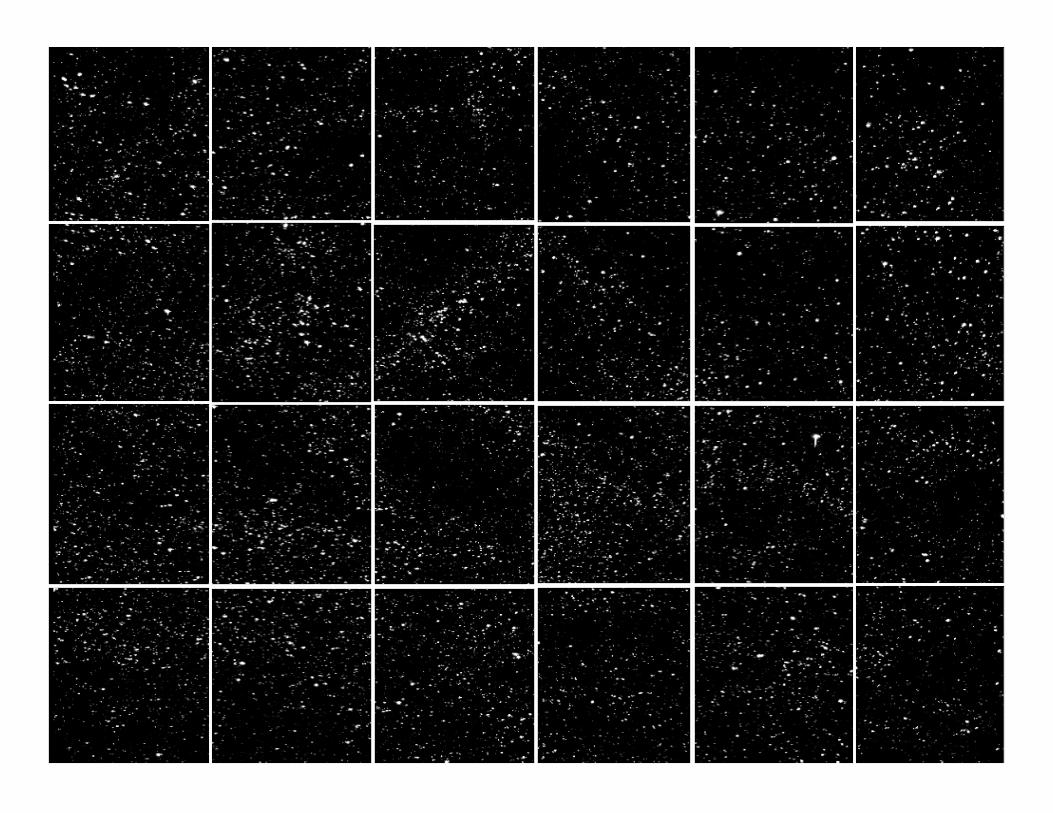
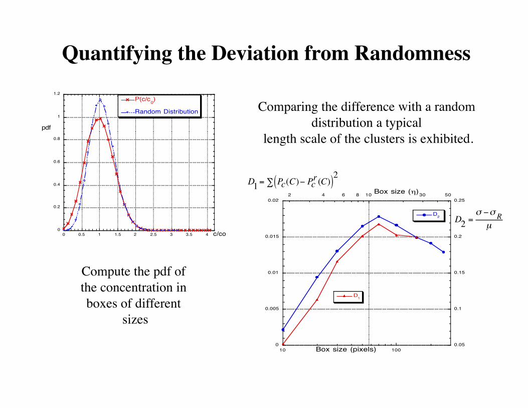
Quantifying the Deviation from Randomness

0

0.005

0.01

0.015

0.02

0.05

0.1

0.15

0.2

0.25

10 100

2 4 6 8 10 30 50

D1

D2

Box size (pixels)

Box size (η)

D2 =σ −σ Rµ

0

0.2

0.4

0.6

0.8

1

1.2

0 0.5 1 1.5 2 2.5 3 3.5 4

P(c/c0)

Random Distribution

pdf

c/co

Compute the pdf of the concentration in boxes of different

sizes

Comparing the difference with a random distribution a typical

length scale of the clusters is exhibited.

D1= Pc(C)− Pcr (C)( )∑

2

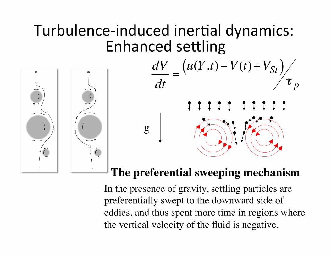
In the presence of gravity, settling particles are preferentially swept to the downward side of eddies, and thus spent more time in regions where the vertical velocity of the fluid is negative.

The preferential sweeping mechanism

g€

dVdt

=u(Y ,t)−V (t)+VSt( )

τ p

Turbulence-inducediner/aldynamics:Enhancedsesling

Downloaded 21 Oct 2009 to 128.95.34.219. Redistribution subject to AIP license or copyright; see http://pof.aip.org/pof/copyright.jsp

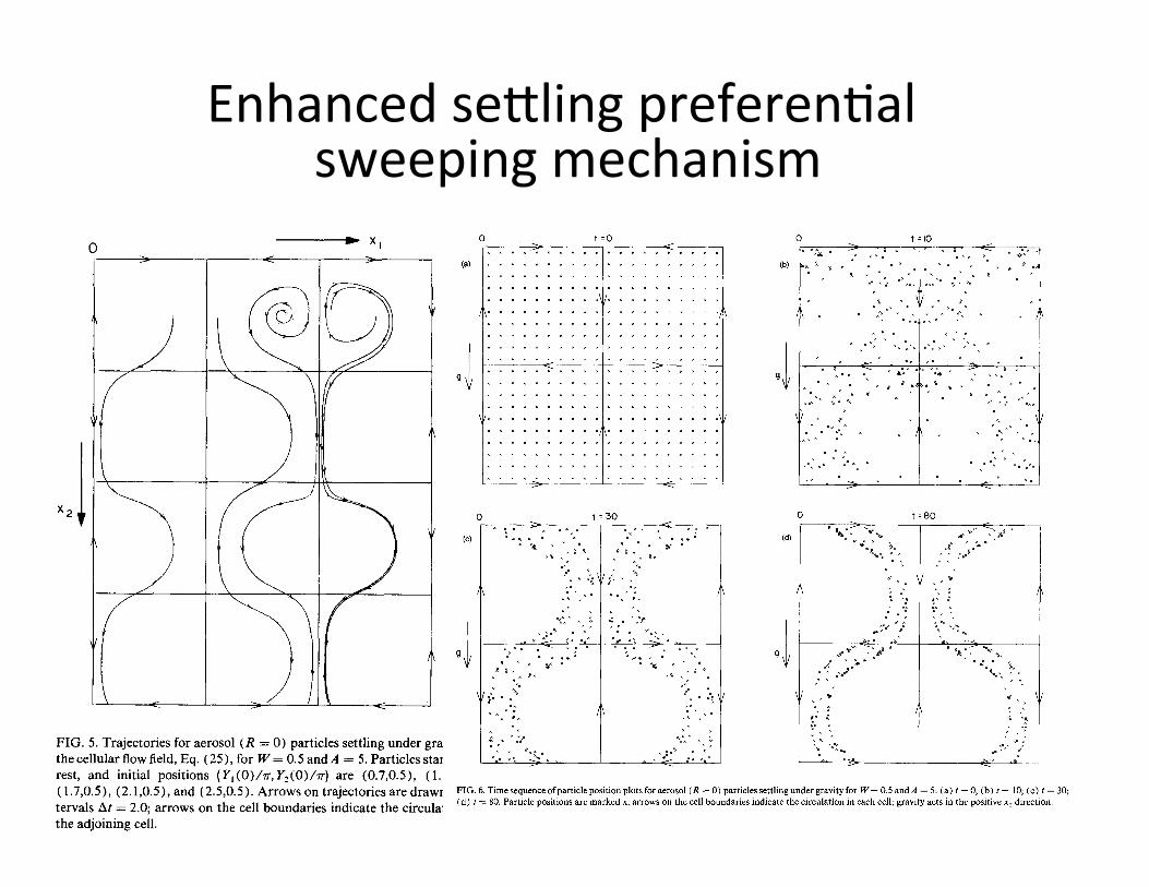
Enhancedseslingpreferen/alsweepingmechanism


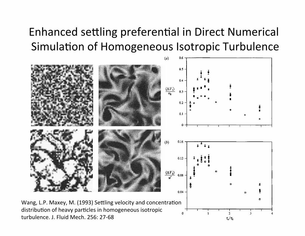
Enhancedseslingpreferen/alinDirectNumericalSimula/onofHomogeneousIsotropicTurbulenceSettling velocity and concentration distribution of particles 45

(a) 0.6

0.5

0.4

@Vl> o.3 vk

0.2

0.1

0 1

0.04 i" 0 1 2 3 4

%/rk

FIGURE 7. The increase (<AV,)) in the particle mean settling velocity as a function of r,/rk for a fixed terminal velocity, W = u,. The error bar represents the statistical uncertainty. (a) Normalized by Kolmogorov velocity scale uk; (b) normalized by r.m.s. fluid velocity u'. 0, 323, Re, = 21; ., 483, Re, = 31 ; 0, 648, Re, = 43; 0, 963, Re, = 62; a, 4g8 and use of the second forcing scheme, Re, = 30. For the 323 simulations, the size of the symbol is made the same as the error bar.

value of 7,/7k at which (AY,)/v, is greatest is consistently within the interval of 0.5 < 7,/7, < 1 and is centred around 0.8 as the Reynolds number Re, is varied. By contrast, the ratio of T,/7, varies from 5.3 to 15.8, so that if the data were presented in terms of the ratio of 7, to T,, which is also representative of Lagrangian integral timescales, then there would be a much greater variation in the location of the peak increase with changing Re,.

These results are also shown in figure 7 where <A 4) is normalized by u'. We see that the quantitative difference among the simulated resulted for different Re, with the first

Wang,L.P.Maxey,M.(1993)Seslingvelocityandconcentra/ondistribu/onofheavypar/clesinhomogeneousisotropicturbulence.J.FluidMech.256:27-68

42 L.-P. Wang and M . R. Maxey

FIGURE 5. Normalized particle concentration (left-hand side) and flow scalar-vorticity field (right- hand side) on an (xl, x,)-slice (x, = 27L/48) at the 5 consecutive time frames. The first frame is at t = 0 when the concentration is uniform. The time interval is 0.018 or about twice the Kolmogorov timescale. The mesh size is 483, Re, = 31, and particle parameters are 7, = 7k, W = vk.

becomes non-uniform as time increases. We present in figure 5 the evolution of a typical normalized concentration field, C/ (C), and the scalar-vorticity field on a slice from the three-dimensional simulation box at five consecutive time frames during the initial development period. The normalized scalar-vorticity Q is defined as (wi wi)i/ ((wiwi);) , where wi is the flow vorticity. Throughout this paper, the grey scale is

42 L.-P. Wang and M . R. Maxey

FIGURE 5. Normalized particle concentration (left-hand side) and flow scalar-vorticity field (right- hand side) on an (xl, x,)-slice (x, = 27L/48) at the 5 consecutive time frames. The first frame is at t = 0 when the concentration is uniform. The time interval is 0.018 or about twice the Kolmogorov timescale. The mesh size is 483, Re, = 31, and particle parameters are 7, = 7k, W = vk.

becomes non-uniform as time increases. We present in figure 5 the evolution of a typical normalized concentration field, C/ (C), and the scalar-vorticity field on a slice from the three-dimensional simulation box at five consecutive time frames during the initial development period. The normalized scalar-vorticity Q is defined as (wi wi)i/ ((wiwi);) , where wi is the flow vorticity. Throughout this paper, the grey scale is

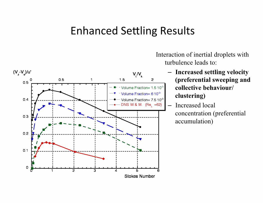
Interaction of inertial droplets with turbulence leads to: –  Increased settling velocity

(preferential sweeping and collective behaviour/clustering)

–  Increased local concentration (preferential accumulation)

EnhancedSeslingResults

-0.15

-0.1

-0.05

0

0.05

0.1

0.15

0 1 2 3 4 5

St=0.03

St=0.05

St=0.07

St=0.11

St=0.19

St=0.55

St=1.10

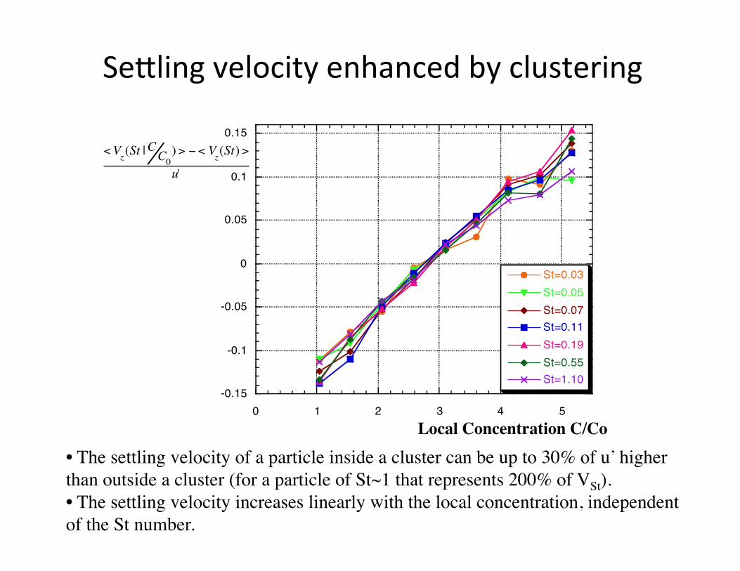
•  The settling velocity of a particle inside a cluster can be up to 30% of u’ higher than outside a cluster (for a particle of St~1 that represents 200% of VSt).•  The settling velocity increases linearly with the local concentration, independent of the St number.

Seslingvelocityenhancedbyclustering

<Vz(St |CC0) > − < Vz(St) >

u'

Local Concentration C/Co

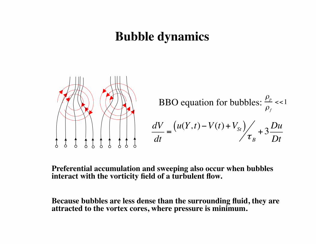
Bubble dynamics

Preferential accumulation and sweeping also occur when bubbles interact with the vorticity field of a turbulent flow.

Because bubbles are less dense than the surrounding fluid, they are attracted to the vortex cores, where pressure is minimum.

BBO equation for bubbles:

dVdt

=u(Y, t)−V (t)+VSt( )

τ B+3Du

Dt

ρpρ f

<<1

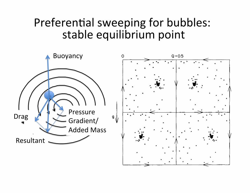
Preferen/alsweepingforbubbles:stableequilibriumpoint


Buoyancy

PressureGradient/AddedMass

Drag

Resultant



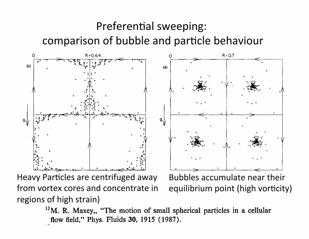
Preferen/alsweeping:comparisonofbubbleandpar/clebehaviour

“H. K. Moffat, “Transport effects associated with turbulence with par- ticular attention to the influence of helicity,” Rep. Prog. Phys. 46, 621 (1983).

‘*M. R. Maxey,, “The motion of small spherical particles in a cellular flow field,” Phys. Fluids 30, 1915 (1987).

I’M. R. Maxey and S. Corrsin, “Gravitational settling of aerosol particles in randomly oriented cellular flow fields,” J. Atmos. Sci. 43, 1112 (1986).

14M. W. Reeks, “Eulerian direct interaction applied to the statistical motion of particles in a turbulent field,” J. Fluid Mech. 97, 569 (1980).

“L. P. Wang and D. E. Stock, “Numerical simulation of heavy particle dispersion--Tie step and nonlinear drag considerations,” ASME J. Fluids Eng. 114, 100 (1992).

16J. R. Rice, Numerical Methods, Softiare and Analysis (McGraw-Hill, New York, 1983).

“A. Wolf, J. B Swift, H. L. Swinney, and J. A. Vastano, “Determining Lyapunov exponents from a time series,” Physica D 16, 285 (1985).

‘sF. Varosi, T. M. Antonsen, and E. Ott, “The spectrum of fractal di- mensions of passively convected scalar gradients in chaotic fluid flows,” Phys. Fluids A 3, 1017 (1991).

19G. I. Taylor, “Diffusion by continuous movements,” Proc. R. Sot. Lon- don Ser. A 151, 421 (1921).

“G. K. Batchelor and A. A. Townsend, “Turbulent diffusion,” Surveys in Mechanics, edited by G. K. Batchelor and R. M. Davies (Cambridge U.P., Cambridge, 1956), pp. 352-399.

“5 D Farmer, E. Ott, and J. A. Yorke, “The dimension of chaotic attractors,” Physica D 7, 153 (1983).

“‘J. Kaplan and J. Yorke, Lecture Notes in Mathematics (Springer- Verlag, New York, 1979), Vol. 730, p. 204.

s3H. Aref, “Stochastic particle motion in laminar flows,” Phys. Fluids A 3, 1009 (1991).

24C. T. Crowe, R. A. Gore, and T. R. Troutt, “Particle dispersion by coherent structures in free shear flows,” Part. Sci. Technol. 3, 149 (1985).

ssB. J. Lazaro and J. C. Lasheras, “Particle dispersion in a turbulent, plane shear layer,” Phys. Fluids A 1, 1035 (1989).

%J. N. Chung and T. R Trout& “Simulations of particle dispersion in an axisymmetric jet,” J. Fluid Mech. 186, 199 (1988).

*‘R. Chein and J. N. Chung, “Simulation of particle dispersion in a two-dimensional mixing layer,” AIChE J. 34, 946 (1988).

“L. P. Wang, M. R. Maxey, and R. Mallier, “Structure of stratified shear layer at high Reynolds numbers,” submitted to Geophys. Astrophys. Fluid Dyn.

29S. Balachandar and M. R. Maxey, “Methods for evaluating fluid velocities in spectral simulations of turbulence,” J. Comput. Phys. 83, 96 (1989).

30G. M. Corcos and F. S. Sherman, “The mixing layer: Deterministic models of a turbulent flow. Part 1. Introduction and the two- dimensional flow,” J. Fluid Mech. 139, 29 (1984).

“Z. Warhaft, “The interference of thermal fields from line sources in grid turbulence,” J. Fluid Mech. 144, 363 ( 1984).

“B. L. Sawford and J. C. R. Hunt, “Effects of turbulent structure, mo- lecular diffusion and source size on scalar fluctuations in homogeneous turbulence,” J. Fluid Mech. 165, 373 (1986).

33D. J. Thomson, “A stochastic model for the motion of particle pairs in isotropic high-Reynolds-number turbulence, and its application to the problem of concentration variance,” J. Fluid Mech. 210, 113 ( 1990).

j4G. I. Taylor, “Dispersion of soluble matter in solvent flowing slowly through a tube,” Proc. R. Sot. London Ser. A 219, 186 (1953).


Bubblesaccumulateneartheirequilibriumpoint(highvor/city)

HeavyPar/clesarecentrifugedawayfromvortexcoresandconcentrateinregionsofhighstrain)

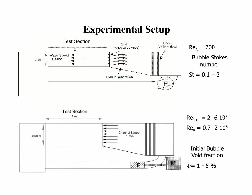
Experimental Setup

Re1 m = 2- 6 105

Reθ = 0.7- 2 103

Initial Bubble Void fraction

Φ= 1 - 5 %

Reλ = 200

Bubble Stokes number

St = 0.1 – 3

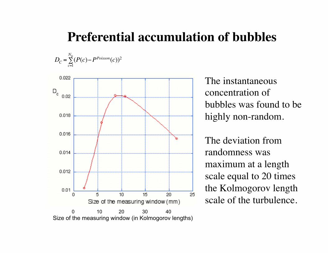
Preferential accumulation of bubbles

The instantaneous concentration of bubbles was found to be highly non-random.The deviation from randomness was maximum at a length scale equal to 20 times the Kolmogorov length scale of the turbulence.

DC = (P(c)−PPoisson(c))2c=1

Nb∑

0 10 20 30 40 Size of the measuring window (in Kolmogorov lengths)

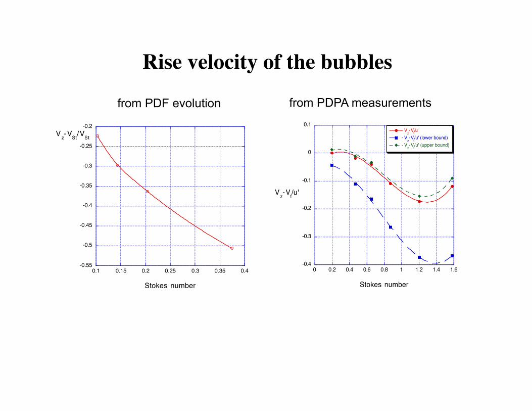
Rise velocity of the bubbles

-0.55

-0.5

-0.45

-0.4

-0.35

-0.3

-0.25

-0.2

0.1 0.15 0.2 0.25 0.3 0.35 0.4

Vz-V

St/V

St

Stokes number

from PDPA measurements

-0.4

-0.3

-0.2

-0.1

0

0.1

0 0.2 0.4 0.6 0.8 1 1.2 1.4 1.6

Rise velocity. U=0.43, C=8.5 10- 4

Vz-V

t/u'

Vz-V

t/u' (lower bound)

Vz-V

t/u' (upper bound)

Vz-V

t/u'

Stokes number

from PDF evolution

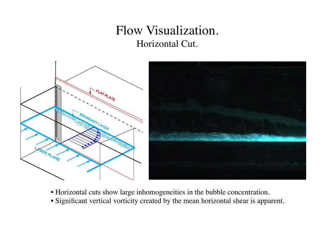
Flow Visualization. �Horizontal Cut.

•  Horizontal cuts show large inhomogeneities in the bubble concentration.•  Significant vertical vorticity created by the mean horizontal shear is apparent.

Bubble clustering due to the turbulent structures

The preferred length scale for accumulation is of the order of 100 wall units (δ+ = ν / uτ )

324 A. Aliseda and J. C. Lasheras

0.02

0.03

0.04

0.05

0.18

0.20

0.22

0.24

0.26

0.28

0.30

0.32

0 100 200 300 400 500

Dsu

m =

Σ(P

– P

pois

son)

2

Dsi

gma

= (σ

– σ

pois

son)

/λ

Window size, [δ+]

Figure 19. Bubble accumulation as a function of the length scale. Indicators defined inequations (3.2) and (3.3). (i) Dsigma = (σ − σpoisson)/λ; (ii) Dsum = Σ(P − Ppoisson)2.

the turbulent structures present in the flow. The algorithm used to identify bubbleclustering by the turbulence consists of the following steps. First, each image is dividedinto square windows of a certain size. The number of bubbles within each of these non-overlapping windows is counted and recorded. With the information correspondingto all the windows covering every image taken under a given condition, we cancompute the density function for the probability of finding a number of bubblesP (nb) in each one of these windows. If the bubbles were passive scalars, their spatialconcentration due to the random stirring of the turbulence would correspond to aPoisson distribution.

Ppoisson(n) =e−λ λn

n!, (3.1)

where λ is the mean number of particles per window, Nb/Nw . By comparing theobserved probability density function with the theoretical Poisson PDF resulting froma purely random process, it is then possible to quantify how the bubble concentrationfield deviates from randomness. By repeating this algorithm for different windowsizes, the dependency of this deviation on the length scale can be determined. Twodifferent ways of comparing the PDFs were employed to quantify the extent of bubbleclustering in the boundary layer. Their definitions, due to Wang & Maxey (1993a)and Fessler, Kulick & Eaton (1994) respectively, are as follows:

Dsum =Nb∑

n=1

(P (nb) − Ppoisson(nb))2, (3.2)

Dsigma =σ − σpoisson

λ, (3.3)

where P (n) is the probability of finding n bubbles in a window, and σpoisson is thestandard deviation of the Poisson distribution.

The values of these quantities, computed for many different window sizes areplotted in figure 19. Both indicators of preferential accumulation reach a maximum

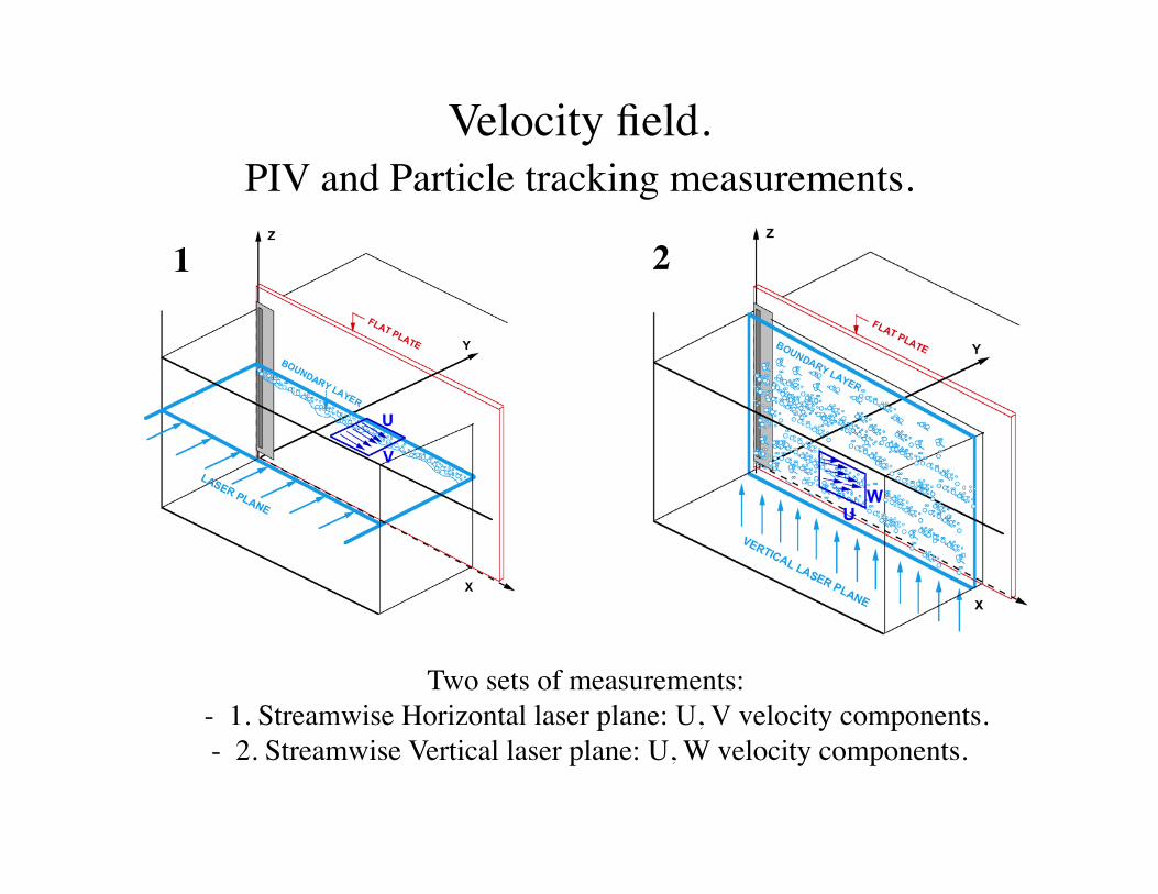
Velocity field.�PIV and Particle tracking measurements.

Two sets of measurements: �- 1. Streamwise Horizontal laser plane: U, V velocity components.�- 2. Streamwise Vertical laser plane: U, W velocity components.

1 2

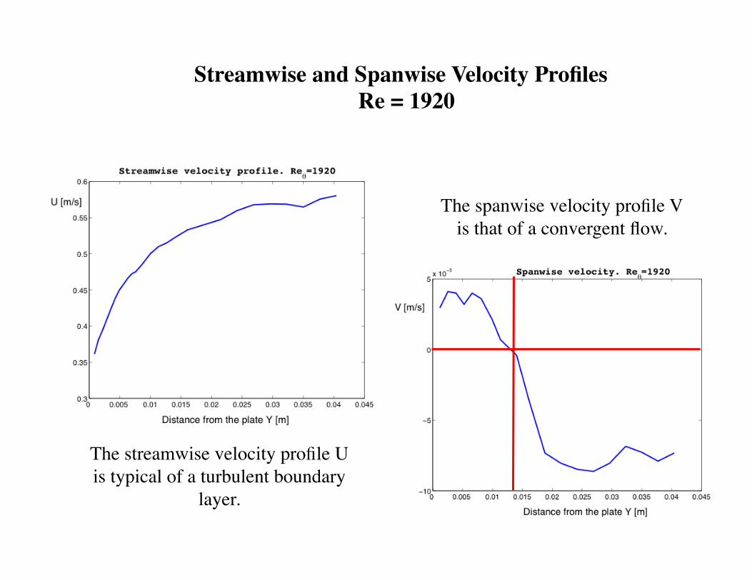
Streamwise and Spanwise Velocity Profiles Re = 1920

The streamwise velocity profile U is typical of a turbulent boundary

layer.

The spanwise velocity profile V is that of a convergent flow.

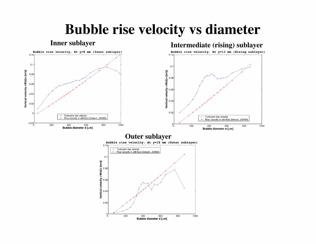
Bubble rise velocity vs diameterInner sublayer Intermediate (rising) sublayer

Outer sublayer

Physics of the interac/ons between iner/al par/cles and ...

Documents

Transcript of Physics of the interac/ons between iner/al par/cles and ...