ON THE EVOLUTION OF A HERMITIAN METRIC … g0 is Ka¨hler (meaning d ω0 = 0), the Ricci flow does...
37
arXiv:1201.0312v3 [math.DG] 19 Jun 2014 ON THE EVOLUTION OF A HERMITIAN METRIC BY ITS CHERN-RICCI FORM VALENTINO TOSATTI ∗ AND BEN WEINKOVE † Abstract. We consider the evolution of a Hermitian metric on a com- pact complex manifold by its Chern-Ricci form. This is an evolution equation first studied by M. Gill, and coincides with the K¨ ahler-Ricci flow if the initial metric is K¨ ahler. We find the maximal existence time for the flow in terms of the initial data. We investigate the behavior of the flow on complex surfaces when the initial metric is Gauduchon, on complex manifolds with negative first Chern class, and on some Hopf manifolds. Finally, we discuss a new estimate for the complex Monge- Amp` ere equation on Hermitian manifolds. 1. Introduction Let (M,J ) be a compact complex manifold of complex dimension n. Let g 0 be a Hermitian metric on M , that is a Riemannian metric g 0 satisfying g 0 (JX,JY )= g 0 (X,Y ) for all vectors X, Y . In local complex coordinates (z 1 ,...,z n ), the metric g 0 is given by a Hermitian matrix with components (g 0 ) i j . Associated to g 0 is a real (1, 1) form ω 0 = √ −1(g 0 ) i j dz i ∧ d z j , which we will also often refer to as a Hermitian metric. Given the success of Hamilton’s Ricci flow [22] in establishing deep results in the setting of topological, smooth and Riemannian manifolds (see e.g. [5, 23, 30]), it is natural to ask whether there is a parabolic flow of metrics on M which starts at g 0 , preserves the Hermitian condition and reveals information about the structure of M as a complex manifold. In the case when g 0 is K¨ ahler (meaning dω 0 = 0), the Ricci flow does precisely this. It gives a flow of K¨ ahler metrics whose behavior is deeply intertwined with the complex and algebro-geometric properties of M (see [8, 9, 15, 31, 32, 34, 35, 36, 37, 38, 40, 41, 45, 50, 51, 52, 56], for example). However, if g 0 is not K¨ ahler, then in general the Ricci flow does not pre- serve the Hermitian condition g(JX,JY )= g(X,Y ). Alternative parabolic flows on complex manifolds which do preserve the Hermitian property have been proposed by Streets-Tian [42, 43] and also Liu-Yang [28]. ∗ Supported in part by NSF grant DMS-1005457 and by a Blavatnik Award for Young Scientists. Part of this work was carried out while the first-named author was visiting the Mathematical Science Center of Tsinghua University in Beijing, which he would like to thank for its hospitality. † Supported in part by NSF grant DMS-1105373. 1
Transcript of ON THE EVOLUTION OF A HERMITIAN METRIC … g0 is Ka¨hler (meaning d ω0 = 0), the Ricci flow does...
arX
iv:1
201.
0312
v3 [
mat
h.D
G]
19
Jun
2014
ON THE EVOLUTION OF A HERMITIAN METRIC BY
ITS CHERN-RICCI FORM
VALENTINO TOSATTI∗ AND BEN WEINKOVE†
Abstract. We consider the evolution of a Hermitian metric on a com-pact complex manifold by its Chern-Ricci form. This is an evolutionequation first studied by M. Gill, and coincides with the Kahler-Ricciflow if the initial metric is Kahler. We find the maximal existence timefor the flow in terms of the initial data. We investigate the behavior ofthe flow on complex surfaces when the initial metric is Gauduchon, oncomplex manifolds with negative first Chern class, and on some Hopfmanifolds. Finally, we discuss a new estimate for the complex Monge-Ampere equation on Hermitian manifolds.
1. Introduction
Let (M,J) be a compact complex manifold of complex dimension n. Letg0 be a Hermitian metric on M , that is a Riemannian metric g0 satisfyingg0(JX, JY ) = g0(X,Y ) for all vectors X, Y . In local complex coordinates(z1, . . . , zn), the metric g0 is given by a Hermitian matrix with components(g0)ij . Associated to g0 is a real (1, 1) form ω0 =
√−1(g0)ijdzi ∧ dzj, which
we will also often refer to as a Hermitian metric.Given the success of Hamilton’s Ricci flow [22] in establishing deep results
in the setting of topological, smooth and Riemannian manifolds (see e.g.[5, 23, 30]), it is natural to ask whether there is a parabolic flow of metricson M which starts at g0, preserves the Hermitian condition and revealsinformation about the structure of M as a complex manifold. In the casewhen g0 is Kahler (meaning dω0 = 0), the Ricci flow does precisely this. Itgives a flow of Kahler metrics whose behavior is deeply intertwined with thecomplex and algebro-geometric properties of M (see [8, 9, 15, 31, 32, 34, 35,36, 37, 38, 40, 41, 45, 50, 51, 52, 56], for example).
However, if g0 is not Kahler, then in general the Ricci flow does not pre-serve the Hermitian condition g(JX, JY ) = g(X,Y ). Alternative parabolicflows on complex manifolds which do preserve the Hermitian property havebeen proposed by Streets-Tian [42, 43] and also Liu-Yang [28].
∗Supported in part by NSF grant DMS-1005457 and by a Blavatnik Award for YoungScientists. Part of this work was carried out while the first-named author was visiting theMathematical Science Center of Tsinghua University in Beijing, which he would like tothank for its hospitality.
†Supported in part by NSF grant DMS-1105373.
1
2 V. TOSATTI AND B. WEINKOVE
This paper is concerned with another such flow, first investigated by M.Gill [19], which we will call the Chern-Ricci flow :
(1.1)∂
∂tω = −Ric(ω), ω|t=0 = ω0,
where here Ric(ω) is the Chern-Ricci form (sometimes called the first Chernform) associated to the Hermitian metric g, which in local coordinates isgiven by
(1.2) Ric(ω) = −√−1∂∂ log det g.
In the case when g is Kahler, Ric(ω) =√−1Rijdzi ∧ dzj, where Rij is the
usual Ricci curvature of g. Thus if g0 is Kahler, (1.1) coincides with theKahler-Ricci flow. In general, Ric(ω) does not have a simple relationshipwith the Ricci curvature of g. The Bott-Chern cohomology class determinedby the closed form Ric(ω) is denoted by cBC
1 (M). We call this the first Bott-Chern class of M . It is independent of the choice of Hermitian metric ω(see section 2 for more details).
The following result for the Chern-Ricci flow was proved by Gill [19]:
Theorem 1.1 (Gill). If cBC1 (M) = 0 then, for any initial metric ω0, there
exists a solution ω(t) to the Chern-Ricci flow (1.1) for all time and the met-rics ω(t) converge smoothly as t → ∞ to a Hermitian metric ω∞ satisfyingRic(ω∞) = 0.
Moreover, the Hermitian metric ω∞ is the unique Chern-Ricci flat metriconM of the form ω∞ = ω0+
√−1∂∂ϕ for some function ϕ. The Chern-Ricci
flat metrics were already known to exist [10, 54], and the estimate of [54] isused in the proof of Theorem 1.1. If ω0 is Kahler then Theorem 1.1 is due toCao [8], with ω∞ being the Ricci-flat metric of Yau [60]. In Section 2 below,we discuss the work of Gill [19] further, and also explain how the Chern-Ricci flow compares with some other parabolic flows on complex manifoldsstudied in the literature.
Our first result characterizes the maximal existence time for a solutionto the Chern-Ricci flow using information from the initial Hermitian metricω0. First observe that the flow equation (1.1) may be rewritten as
∂
∂tω = −Ric(ω0) +
√−1∂∂θ(t), with θ(t) = log
det g(t)
det g0.
Thus, as long as the flow exists, the solution ω(t) starting at ω0 must be ofthe form ω(t) = αt +
√−1∂∂Θ, for some function Θ = Θ(t), with
(1.3) αt = ω0 − tRic(ω0).
Now define a number T = T (ω0) with 0 < T 6 ∞ by
(1.4) T = supt > 0 | ∃ψ ∈ C∞(M) with αt +√−1∂∂ψ > 0.
By the observation above, a solution to (1.1) cannot exist beyond time T .We prove:
EVOLUTION OF A HERMITIAN METRIC BY ITS CHERN-RICCI FORM 3
Theorem 1.2. There exists a unique maximal solution to the Chern-Ricciflow (1.1) on [0, T ).
In the special case when ω0 is Kahler, this is already known by the resultof Tian-Zhang [51], who extended earlier work of Cao and Tsuji [8, 56, 57].In the Kahler case, T depends only on the cohomology class [ω0] and can bewritten
T = supt > 0 | [ω0]− tc1(M) > 0.Furthermore the Nakai-Moishezon criterion, due to Buchdahl [7] and Lamari[25] for Kahler surfaces and to Demailly-Paun [11] for general Kahler man-ifolds, implies that at time T either the volume of M goes to zero, or thevolume of some proper analytic subvariety of M goes to zero (cf. the dis-cussion in [15]).
Note that in the general Hermitian case, we can consider the equivalencerelation of (1, 1) forms on M :
α ∼ α′ ⇐⇒ α = α′ +√−1∂∂ψ for some function ψ ∈ C∞(M).
Then T defined by (1.4) depends only on the equivalence class of ω0.In the special case when M is a complex surface (n = 2) a result of
Gauduchon [16] is that every Hermitian metric is conformal to a ∂∂-closedmetric ω0. If ω0 is ∂∂-closed then so is ω(t) for t ∈ [0, T ). Moreover, wehave a geometric characterization of the maximal existence time T :
Theorem 1.3. Let M be a compact complex surface, ω0 a ∂∂-closed Her-mitian metric. Then T defined by (1.4) can be written as
T = sup
T0 > 0
∣
∣
∣
∣
∀t ∈ [0, T0],
∫
Mα2t > 0,
∫
Dαt > 0,
for all D irreducible effective divisors with D2 < 0
,
for αt given by (1.3).
Note that for t ∈ [0, T ), the quantity∫
M α2t =
∫
M ω(t)2 is the volume ofM (with respect to ω(t)) and
∫
D αt =∫
D ω(t) is the volume of the curve D.Thus we can restate Theorem 1.3 as:
Corollary 1.4. Let M be a compact complex surface, ω0 a ∂∂-closed Her-mitian metric. Then the Chern-Ricci flow (1.1) starting at ω0 exists untileither the volume of M goes to zero, or the volume of a curve of negativeself-intersection goes to zero.
As we remarked above, the same result was known to hold for the Kahler-Ricci flow thanks to the Nakai-Moishezon criterion of [7, 25]. Analogues ofTheorems 1.2, 1.3 and Corollary 1.4 were conjectured by Streets-Tian [44]for their pluriclosed flow (see Section 2 below).
The Kahler-Ricci flow has a deep connection to the Minimal Model Pro-gram in algebraic geometry, as demonstrated by the work of Song-Tian and
4 V. TOSATTI AND B. WEINKOVE
others [14, 26, 34, 35, 36, 37, 38, 39, 40, 41, 50, 51, 56, 63]. In the case ofalgebraic surfaces, the minimal model program is relatively simple. Indeed,a minimal surface is defined to be a surface with no (−1)-curves (smoothrational curves C with C2 = −1). To find the minimal model, one can justapply a finite number of blow-downs, which are algebraic operations con-tracting the (−1)-curves. It was shown in [38] that the Kahler-Ricci flowon an algebraic surface carries out these algebraic operations, contracting(−1)-curves in the sense of Gromov-Hausdorff, and smoothly outside of thecurves. Moreover, the same behavior occurs on a non-algebraic Kahler sur-face [40]. In all dimensions, weak solutions to the Kahler-Ricci flow throughsingularites were constructed in [36] and a number of conjectures were madeabout the metric behavior of the flow (see also [41]).
We return now to the case of a complex (non-Kahler) surface. In thiscase one can also contract the (−1) curves to arrive at a minimal surface.We conjecture that the Chern-Ricci flow on a complex surface starting at a∂∂-closed metric behaves in an analogous way to the Kahler-Ricci flow on aKahler surface. We prove the following:
Theorem 1.5. Let M be a compact complex surface with a ∂∂-closed Her-mitian metric ω0, and let [0, T ) be the maximal existence time of the Chern-Ricci flow starting from ω0. Then
(a) If T = ∞ then M is minimal(b) If T < ∞ and Vol(M,ω(t)) → 0 as t → T−, then M is either
birational to a ruled surface or it is a surface of class V II (and inthis case it cannot be an Inoue surface)
(c) If T < ∞ and Vol(M,ω(t)) stays positive as t → T−, then M con-tains (−1)-curves.
Furthermore, if M is minimal then T = ∞ unlessM is CP2, a ruled surface,a Hopf surface or a surface of class VII with b2 > 0, in which cases (b) holds.
In the case that M is not minimal, and (c) occurs, we expect that theChern-Ricci flow will contract a finite number of (−1)-curves and can beuniquely continued on the new manifold. Moreover, we conjecture that thisprocess can be repeated until one obtains a minimal surface, or ends up incase (b) above. More details of this conjecture can be found in Section 6.
To provide some evidence for our conjecture, we prove the following the-orem. It is an analogue of a result for the Kahler-Ricci flow, whose proof isessentially contained in [51] (for a recent exposition, see Chapter 7 of [40]),and which was a key starting point for the work [36, 37, 38, 39]. We assumethat the maximal existence time T is finite and, roughly speaking, that thelimiting ‘class’ of the flow at time T is given by the pull-back of a Hermitianmetric on a manifold N via π : M → N , where π is a holomorphic mapblowing down an exceptional divisor E to a point p ∈ N . We show that thesolution to the Chern-Ricci flow will converge smoothly at time T away fromE. In this way, one can obtain a Hermitian metric on the new manifold N ,at least away from the point p. Our result holds in any dimension:
EVOLUTION OF A HERMITIAN METRIC BY ITS CHERN-RICCI FORM 5
Theorem 1.6. Assume that there exists a holomorphic map between com-pact Hermitian manifolds π : (M,ω0) → (N,ωN ) blowing down the excep-tional divisor E on M to a point p ∈ N . In addition, assume that thereexists a smooth function ψ on M with
(1.5) ω0 − TRic (ω0) +√−1∂∂ψ = π∗ωN ,
with T <∞ given by (1.4).Then the solution ω(t) to the Chern-Ricci flow (1.1) starting at ω0 con-
verges in C∞ on compact subsets of M \ E to a smooth Hermitian metricωT on M \ E.
There are some new obstacles to proving this in the non-Kahler case thatwe overcome using a parabolic Schwarz Lemma for volume forms, and asecond order estimate for the metric which uses a trick of Phong-Sturm [33].
In the cases when the flow has a long time solution, it is natural toinvestigate its behavior at infinity. If the manifold has vanishing first Bott-Chern class, we have already seen by Gill’s result (Theorem 1.1) that theflow converges to a Chern-Ricci flat Hermitian metric. We now supposethat the first Chern class c1(M) is negative (note that cBC
1 (M) < 0 impliesc1(M) < 0). In this case, the manifoldM is Kahler and a fundamental resultof Aubin [1] and Yau [60] says that M admits a unique Kahler-Einsteinmetric ωKE with negative scalar curvature. Cao [8] then proved that theKahler-Ricci flow (appropriately normalized) deforms any Kahler metric in−c1(M) to ωKE. The same is true for the normalized Kahler-Ricci flowstarting at any Kahler metric [51, 56]. Our next result shows that startingat any Hermitian metric on the manifold M , the (normalized) Chern-Ricciflow will converge to the Kahler-Einstein metric ωKE.
Theorem 1.7. Let M be a compact complex manifold with c1(M) < 0 andlet ω0 be a Hermitian metric on M . Then the Chern-Ricci flow (1.1) has along-time solution ω(t), and as t goes to infinity the rescaled metrics ω(t)/tconverge smoothly to the unique Kahler-Einstein metric ωKE on M .
In particular we see that the Chern-Ricci flow on these manifolds, afternormalization, deforms any Hermitian metric to a Kahler one.
Next we illustrate the Chern-Ricci flow with an explicit example. Forα = (α1, . . . , αn) ∈ C
n \ 0 with |α1| = · · · = |αn| 6= 1, we consider theHopf manifold Mα = (Cn \ 0)/ ∼ where
(z1, . . . , zn) ∼ (α1z1, . . . , αnzn).
This is a non-Kahler complex manifold of complex dimension n. If n = 2, itis an example of a class VII surface. We can write down an exact solution
to the Chern-Ricci flow on Mα. Consider the metric ωH =δijr2
√−1dzi ∧ dzj.
Then we have:
Proposition 1.8. The metrics ω(t) := ωH−tRic (ωH) onMα give a solutionof the Chern-Ricci flow on the maximal existence interval [0, 1/n). As t →
6 V. TOSATTI AND B. WEINKOVE
T = 1/n, the limiting nonnegative (1, 1) form ωT is given by
ωT =zizjr4
√−1dzi ∧ dzj .
In the case of the original Hopf surface, which has α = (2, 2) and is anelliptic fiber bundle over P1 via the map (z1, z2) 7→ [z1, z2], the limiting formωT is positive definite along the fibers and zero in directions orthogonal tothe fibers.
If we start with any metric ω0 which differs from ωH by√−1∂∂ψ for some
function ψ, then we conjecture that the flow also converges as t → T to asmooth but degenerate (1, 1) form on Mα with properties similar to ωT . Togive evidence for this conjecture, we prove an estimate:
Proposition 1.9. Let ω0 = ωH +√−1∂∂ψ be a Hermitian metric on Mα,
and let ω(t) be the solution of the Chern-Ricci flow (1.1) starting at ω0 onMα for t ∈ [0, 1/n). Then there exists a uniform constant C such that
ω(t) 6 CωH , for t ∈ [0, 1/n).
In particular, this result shows that we obtain convergence for the flow atthe level of potential functions in C1+β for any β ∈ (0, 1). For more detailssee Section 8.
The final result in this paper concerns not the Chern-Ricci flow, but anelliptic equation: the complex Monge-Ampere equation
(1.6) (ω +√−1∂∂ϕ)n = eFωn, ω′ := ω +
√−1∂∂ϕ > 0,
on a compact Hermitian manifold (M,ω), where F is a smooth function onM . We give an alternative proof of a result of [54] that ‖ϕ‖C0 is uniformlybounded (see also [4, 12]). The result makes use of a new second order es-timate in this context: trωω
′ 6 CeA(ϕ−infM ϕ) which we conjectured to holdin [53]. For more details see Section 9. We have included this result herebecause it follows easily from the argument used in Theorem 1.6 togetherwith the method of [53]. The key new ingredient is the trick of Phong-Sturm[33] applied to this setting.
2. Preliminaries and comparison with other flows
In this section, we include for the reader’s convenience some backgroundmaterial on local coordinate computations with Hermitian metrics.
Let (M,g) be a compact Hermitian manifold of complex dimension n.We will often compute in complex coordinates z1, . . . , zn. In this case, gis determined by the n × n Hermitian matrix gij = g(∂i, ∂j), where we are
writing ∂i, ∂j for ∂∂zi, ∂∂zj
respectively. We denote by gji the entries of the
inverse matrix of (gij).We define the Chern connection ∇ associated to g as follows. Given a
vector field X = Xi∂i and a (1, 0) form a = aidzi, we define ∇X and ∇a to
EVOLUTION OF A HERMITIAN METRIC BY ITS CHERN-RICCI FORM 7
be the tensors with components:
∇iXk = ∂iX
k + ΓkijX
j , ∇iaj = ∂iaj − Γkijak,
where the Christoffel symbols Γkij are given by
Γkij = gqk∂igjq.
The tensors ∇X and ∇a have components ∇iXk = ∂iXk and ∇iaj = ∂iaj.The connection ∇ can be naturally extended to any kind of tensor, and wehave ∇kgij = 0.
We write ∆ for the complex Laplacian of g, which acts on a function f by
∆f = gji∂i∂jf = gji∇i∇jf.
The torsion of g is the tensor T with components
T kij = Γk
ij − Γkji.
The torsion tensor vanishes in the special case that g is Kahler.We define the curvature of g to be the tensor with components
R p
kℓi= −∂ℓΓ
pki.
We will often raise and lower indices using the metric g, writing for ex-ample Rkℓij = gpjR
p
kℓi. Note that Rkℓij = Rℓkji. We have the following
commutation formulae:
[∇k,∇ℓ]Xi = R i
kℓjXj , [∇k,∇ℓ]X
i = −R ikℓ j
Xj ,
[∇k,∇ℓ]aj = −R ikℓj
ai, [∇k,∇ℓ]aj = R ikℓ j
ai,
where we are writing [∇k,∇ℓ] for ∇k∇ℓ −∇ℓ∇k. We write the Chern-Ricci
curvature of g as the tensor RCkℓ
given by
RCkℓ
= gjiRkℓij = −∂k∂ℓ log det g,so that the Chern-Ricci form is equal to
Ric(ω) =√−1RC
kℓdzk ∧ dzℓ.
It is a closed real (1, 1) form and its cohomology class in the Bott-Cherncohomology group
H1,1BC(M,R) =
closed real (1, 1) forms√−1∂∂ψ, ψ ∈ C∞(M,R)
,
is the first Bott-Chern class of M , and is denoted by cBC1 (M). It is indepen-
dent of the choice of Hermitian metric ω. More generally, if Ω is a smoothpositive volume form on M we can define locally Ric(Ω) = −
√−1∂∂ log Ω,
which is a global closed real (1, 1) form that represents cBC1 (M). For no-
tational convenience, we omit the factor of 2π that usually appears in thedefinition of cBC
1 (M). The downside of this convention is that some factorsof 2π will appear later in the cohomological calculations of Section 6.
8 V. TOSATTI AND B. WEINKOVE
We end this section by briefly mentioning some related parabolic equa-tions on Hermitian manifolds which have previously been studied in theliterature. Streets-Tian [43] introduced the flow
(2.1)∂
∂tgij = −Sij +Qij , g|t=0 = g0,
where Sij is given by taking ‘the other trace’ of the curvature of the Chernconnection:
Sij = gℓkRkℓij ,
and Qij is a certain quadratic term in the torsion. If the form ω0 associated
to g0 satisfies ∂∂ω0 = 0, this equation becomes their pluriclosed flow
(2.2)∂
∂tω = ∂∂∗ω + ∂ ∂
∗
ω − Ric(ω), ω|t=0 = ω0,
and if g0 is Kahler, it coincides with the Kahler-Ricci flow. They analyzed(2.2) in detail in [42, 44] and made a number of conjectures about it, two ofwhich are analogues of our Theorems 1.2 and 1.3. They conjecture that theirflow can be used to study the topology of class VII+ surfaces. In addition,Streets-Tian considered a family of flows of the form (2.1) with arbitraryquadratic torsion term Q and proved, among other results, a short-timeexistence theorem [43]. The flow (2.1) was extended to the almost complexsetting by Vezzoni [58]. Liu-Yang [28] propose studying the flow (2.1) in thecase of Q = 0.
In [19], Gill introduced the following parabolic complex Monge-Ampereequation on a compact Hermitian manifold (M, g):
(2.3)∂
∂tϕ = log
det(gij + ∂i∂jϕ)
det(gij)− F, gij + ∂i∂jϕ > 0, ϕ|t=0 = 0,
for a fixed smooth function F on M . He showed that the unique solution to(2.3) exists for all time and, after an appropriate normalization, converges inC∞ to a smooth function ϕ∞ solving the complex Monge-Ampere equation
(2.4) logdet(gij + ∂i∂jϕ∞)
det(gij)= F + b,
for a constant b which is uniquely determined. The existence of solutionsto the elliptic equation (2.4) on Hermitian manifolds (generalizing Yau’sTheorem [60]) was already known by the work of Cherrier [10] (if n = 2)and the authors [54] (n > 2). See also [21, 62]. In the special case where gis Kahler, the flow (2.3) had been considered earlier by Cao [8], who provedthe analogous results.
In the case when cBC1 (M) = 0, we can find a function F satisfying
∂∂ log det g = ∂∂F,
and with this choice, ω(t) = ω+√−1∂∂ϕ(t) for ϕ(t) solving (2.3) is exactly
the Chern-Ricci flow starting at ω. In general, the only difference betweenthe Chern-Ricci flow and Gill’s flow (2.3) is that for the Chern-Ricci flow
EVOLUTION OF A HERMITIAN METRIC BY ITS CHERN-RICCI FORM 9
we replace the fixed metric g by a smoothly varying family of Hermitianmetrics gt, and replace F by a particular function, which may also dependon t. Many of Gill’s estimates carry over easily to the case of the Chern-Ricciflow and we will make extensive use of them here.
A final remark about notation. In the following, C,C ′ will denote uniformpositive constants which may vary from line to line.
3. Evolution of the trace of the metric
In this section we write down a formula for the evolution of the trace ofthe evolving metric with respect to a fixed Hermitian metric. We will needthis calculation in later sections. We carry out the computation here usingtensorial quantities, following [10], rather than using a particular choice ofcomplex coordinates as in [19, 21, 43, 53], for example.
We suppose that we have three Hermitian metrics g, g0 and g such thatg = g(t) satisfies the Chern-Ricci flow (1.1), and such that the correspondingforms satisfy
(3.1) ω = ω0 + η(t),
for a closed (1, 1) form η(t).
We denote by ∇, T , Γ, R the Chern connection, torsion, Christoffel sym-bols and curvature of g. Denote by T0 the torsion tensor of g0 and by ∆ thecomplex Laplacian associated to g = g(t).
Note that for the purposes of this paper we will in fact only need the caseof g = g0. However, we included the more general calculation below sincewe anticipate that it may be useful in the future.
We have:
Proposition 3.1. The evolution of log trgg is given by(
∂
∂t−∆
)
log trgg = (I) + (II) + (III)(3.2)
where
(I) =1
trgg
[
− gjpgqigℓk∇kgij∇ℓgpq +1
trgggℓk∇ktrgg∇ℓtrgg
− 2Re(
gjigℓkT pki∇ℓgpj
)
− gjigℓkT pikT
qjℓgpq
]
(II) =1
trgg
[
gjigℓk(∇iTqjℓ − Riℓpj g
qp)gkq
]
(III) = − 1
trgg
[
gjigℓk(
∇i
(
(T0)pjℓ(g0)kp
)
+ ∇ℓ
(
(T0)pik(g0)pj
))
− gjigℓkT qjℓ(T0)
pik(g0)pq
]
.
10 V. TOSATTI AND B. WEINKOVE
Moreover we have
(I) 62
(trgg)2Re(
gℓigqk(T0)pki(g0)pℓ∇qtrgg
)
,
(II) 6 Ctrgg,
for a constant C that depends only on g. If we are at a point where trgg > 1,then
(III) 6 C ′trg g,
for C ′ depending only on g0 and g.
Proof. First,
∆trgg = gji∇i∇j(gℓkgkℓ) = gjigℓk∇i∇jgkℓ.
From the definition of covariant derivative,
∇jgkℓ = ∂jgkℓ − Γpjℓgkp,
and skew-symmetrizing in j, ℓ
∇jgkℓ = ∇ℓgkj + (∂ω)jkℓ − T pjℓgkp.
But from (3.1), ∂ω = ∂ω0, and we may rewrite this in terms of the torsion
of g0 as (∂ω0)jkℓ = (T0)pjℓ(g0)kp. Thus
∇i∇jgkℓ = ∇i∇ℓgkj + ∇i
(
(T0)pjℓ(g0)kp
)
− (∇iTqjℓ)gkq − T q
jℓ∇igkq.
Switching covariant derivatives
∇i∇ℓgkj = ∇ℓ∇igkj − Riℓkqgqpgpj + Riℓpj g
qpgkq.
Arguing as above,
∇ℓ∇igkj = ∇ℓ∇kgij + ∇ℓ
(
(T0)pik(g0)pj
)
− (∇ℓTpik)gpj − T p
ik∇ℓgpj.
Combining all of these we have
∆trgg = gjigℓk∇ℓ∇kgij + gjigℓk(
∇i
(
(T0)pjℓ(g0)kp
)
+ ∇ℓ
(
(T0)pik(g0)pj
)
− (∇iTqjℓ − Riℓpj g
qp)gkq
− (∇ℓTpik + Riℓkqg
qp)gpj − T qjℓ∇igkq − T p
ik∇ℓgpj
)
.
(3.3)
We will make a change to the second to last term using
(3.4) T qjℓ∇igkq = T q
jℓ∇kgiq + T qjℓ(T0)
pik(g0)pq − T p
ikTqjℓgpq.
On the other hand,
∂
∂ttrgg = gℓk∂k∂ℓ log det(g) = gjigℓk∂k∂ℓgij − gjpgqigℓk∂kgij∂ℓgpq,
EVOLUTION OF A HERMITIAN METRIC BY ITS CHERN-RICCI FORM 11
and we wish to convert the partial derivatives into covariant ones. For this,we use the relations
∂kgij = ∇kgij + Γrkigrj
and
∂ℓ∂kgij = ∂ℓ∇kgij +(
∂ℓΓrki
)
grj + Γrki∂ℓgrj
= ∇ℓ∇kgij + Γsℓj∇kgis − Rkℓiq g
qrgrj + Γrki∇ℓgrj + Γr
kiΓsℓjgrs.
Substituting we get
(3.5)∂
∂ttrgg = gjigℓk∇ℓ∇kgij − gjpgqigℓk∇kgij∇ℓgpq − gℓkgjiRkℓij
and so, combining (3.3), (3.4) and (3.5),(
∂
∂t−∆
)
log trgg
=1
trgg
(
[
− gjpgqigℓk∇kgij∇ℓgpq +1
trgggℓk∇ktrgg∇ℓtrgg
− 2Re(
gjigℓkT pki∇ℓgpj
)
− gjigℓkT pikT
qjℓgpq
]
+
[
gjigℓk(∇iTqjℓ − Riℓpj g
qp)gkq + gℓk(∇ℓTiik + Riℓkq g
qi − Rkℓiq gqi)
]
−[
gjigℓk(
∇i
(
(T0)pjℓ(g0)kp
)
+ ∇ℓ
(
(T0)pik(g0)pj
))
− gjigℓkT qjℓ(T0)
pik(g0)pq
]
)
.
Note that in the first set of square brackets above we have used the identityT pki = −T p
ik. To obtain (3.2) it remains to show that the expression
gℓk(∇ℓTiik + Riℓkq g
qi − Rkℓiq gqi)
in the second set of square brackets vanishes. To see this, note that
Riℓkq − Rkℓiq = −gjq∂ℓTjik = −gjq∇ℓT
jik,
and so
gℓkgqi(Riℓkq − Rkℓiq) = −gℓkgqigjq∇ℓTjik = −gℓk∇ℓT
iik,
so that
(3.6) gℓk(∇ℓTiik + Riℓkq g
qi − Rkℓiq gqi) = 0,
establishing (3.2).We now give the estimates on (I), (II), (III). The bounds on (II) and
(III) follow immediately from the definitions of these quantities. It remainsto prove the bound on (I).
12 V. TOSATTI AND B. WEINKOVE
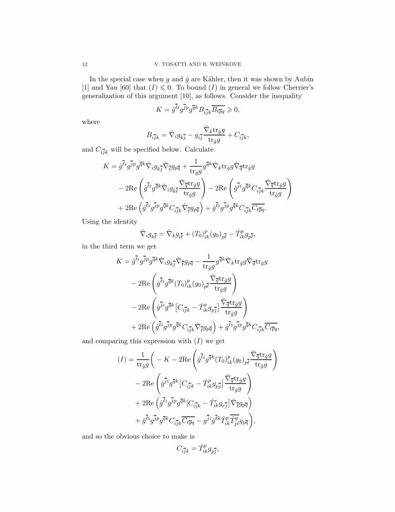
In the special case when g and g are Kahler, then it was shown by Aubin[1] and Yau [60] that (I) 6 0. To bound (I) in general we follow Cherrier’sgeneralization of this argument [10], as follows. Consider the inequality
K = gℓigjpgqkBijkBℓpq > 0,
where
Bijk = ∇igkj − gij∇ktrgg
trgg+ Cijk,
and Cijk will be specified below. Calculate
K = gℓigjpgqk∇igkj∇ℓgpq +1
trgggqk∇ktrgg∇qtrgg
− 2Re
(
gℓigqk∇igkℓ∇qtrgg
trgg
)
− 2Re
(
gjigqkCijk
∇qtrgg
trgg
)
+ 2Re(
gℓigjpgqkCijk∇ℓgpq
)
+ gℓigjpgqkCijkCℓpq.
Using the identity
∇igkℓ = ∇kgiℓ + (T0)pik(g0)pℓ − T p
ikgpℓ,
in the third term we get
K = gℓigjpgqk∇igkj∇ℓgpq −1
trgggqk∇ktrgg∇qtrgg
− 2Re
(
gℓigqk(T0)pik(g0)pℓ
∇qtrgg
trgg
)
− 2Re
(
gjigqk[
Cijk − T pikgpj
]∇qtrgg
trgg
)
+ 2Re(
gℓigjpgqkCijk∇ℓgpq
)
+ gℓigjpgqkCijkCℓpq,
and comparing this expression with (I) we get
(I) =1
trgg
(
−K − 2Re
(
gℓigqk(T0)pik(g0)pℓ
∇qtrgg
trgg
)
− 2Re
(
gjigqk[
Cijk − T pikgpj
]∇qtrgg
trgg
)
+ 2Re(
gℓigjpgqk[Cijk − T rikgrj
]
∇ℓgpq
)
+ gℓigjpgqkCijkCℓpq − gjigℓkT pikT
qjℓgpq
)
,
and so the obvious choice to make is
Cijk = T pikgpj ,
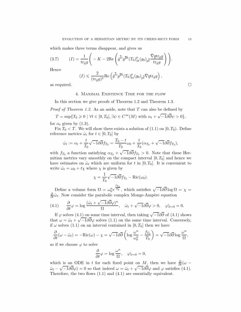
EVOLUTION OF A HERMITIAN METRIC BY ITS CHERN-RICCI FORM 13
which makes three terms disappear, and gives us
(3.7) (I) =1
trgg
(
−K − 2Re
(
gℓigqk(T0)pik(g0)pℓ
∇qtrgg
trgg
))
.
Hence
(I) 62
(trgg)2Re(
gℓigqk(T0)pki(g0)pℓ∇qtrgg
)
,
as required.
4. Maximal Existence Time for the flow
In this section we give proofs of Theorem 1.2 and Theorem 1.3.
Proof of Theorem 1.2. As an aside, note that T can also be defined by
T = supT0 > 0 | ∀t ∈ [0, T0],∃ψ ∈ C∞(M) with αt +√−1∂∂ψ > 0,
for αt given by (1.3).Fix T0 < T . We will show there exists a solution of (1.1) on [0, T0). Define
reference metrics ωt for t ∈ [0, T0] by
ωt := αt +t
T0
√−1∂∂fT0
=T0 − t
T0ω0 +
t
T0(αT0
+√−1∂∂fT0
),
with fT0a function satisfying αT0
+√−1∂∂fT0
> 0. Note that these Her-mitian metrics vary smoothly on the compact interval [0, T0] and hence wehave estimates on ωt which are uniform for t in [0, T0]. It is convenient towrite ωt = ω0 + tχ where χ is given by
χ =1
T0
√−1∂∂fT0
− Ric(ω0).
Define a volume form Ω = ωn0 e
fT0T0 , which satisfies
√−1∂∂ log Ω = χ =
∂∂t ωt. Now consider the parabolic complex Monge-Ampere equation
(4.1)∂
∂tϕ = log
(ωt +√−1∂∂ϕ)n
Ω, ωt +
√−1∂∂ϕ > 0, ϕ|t=0 = 0.
If ϕ solves (4.1) on some time interval, then taking√−1∂∂ of (4.1) shows
that ω = ωt +√−1∂∂ϕ solves (1.1) on the same time interval. Conversely,
if ω solves (1.1) on an interval contained in [0, T0] then we have
∂
∂t(ω − ωt) = −Ric(ω)− χ =
√−1∂∂
(
logωn
ωn0
− fT0
T0
)
=√−1∂∂ log
ωn
Ω,
so if we choose ϕ to solve
∂
∂tϕ = log
ωn
Ω, ϕ|t=0 = 0,
which is an ODE in t for each fixed point on M , then we have ∂∂t(ω −
ωt −√−1∂∂ϕ) = 0 so that indeed ω = ωt +
√−1∂∂ϕ and ϕ satisfies (4.1).
Therefore, the two flows (1.1) and (4.1) are essentially equivalent.
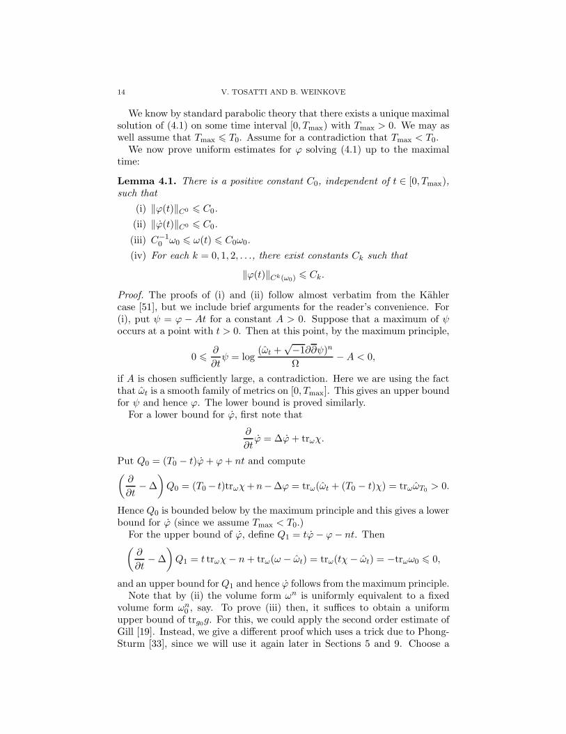
14 V. TOSATTI AND B. WEINKOVE
We know by standard parabolic theory that there exists a unique maximalsolution of (4.1) on some time interval [0, Tmax) with Tmax > 0. We may aswell assume that Tmax 6 T0. Assume for a contradiction that Tmax < T0.
We now prove uniform estimates for ϕ solving (4.1) up to the maximaltime:
Lemma 4.1. There is a positive constant C0, independent of t ∈ [0, Tmax),such that
(i) ‖ϕ(t)‖C0 6 C0.
(ii) ‖ϕ(t)‖C0 6 C0.
(iii) C−10 ω0 6 ω(t) 6 C0ω0.
(iv) For each k = 0, 1, 2, . . ., there exist constants Ck such that
‖ϕ(t)‖Ck(ω0) 6 Ck.
Proof. The proofs of (i) and (ii) follow almost verbatim from the Kahlercase [51], but we include brief arguments for the reader’s convenience. For(i), put ψ = ϕ − At for a constant A > 0. Suppose that a maximum of ψoccurs at a point with t > 0. Then at this point, by the maximum principle,
0 6∂
∂tψ = log
(ωt +√−1∂∂ψ)n
Ω−A < 0,
if A is chosen sufficiently large, a contradiction. Here we are using the factthat ωt is a smooth family of metrics on [0, Tmax]. This gives an upper boundfor ψ and hence ϕ. The lower bound is proved similarly.
For a lower bound for ϕ, first note that
∂
∂tϕ = ∆ϕ+ trωχ.
Put Q0 = (T0 − t)ϕ+ ϕ+ nt and compute(
∂
∂t−∆
)
Q0 = (T0 − t)trωχ+n−∆ϕ = trω(ωt + (T0 − t)χ) = trωωT0> 0.
Hence Q0 is bounded below by the maximum principle and this gives a lowerbound for ϕ (since we assume Tmax < T0.)
For the upper bound of ϕ, define Q1 = tϕ− ϕ− nt. Then(
∂
∂t−∆
)
Q1 = t trωχ− n+ trω(ω − ωt) = trω(tχ− ωt) = −trωω0 6 0,
and an upper bound forQ1 and hence ϕ follows from the maximum principle.Note that by (ii) the volume form ωn is uniformly equivalent to a fixed
volume form ωn0 , say. To prove (iii) then, it suffices to obtain a uniform
upper bound of trg0g. For this, we could apply the second order estimate ofGill [19]. Instead, we give a different proof which uses a trick due to Phong-Sturm [33], since we will use it again later in Sections 5 and 9. Choose a
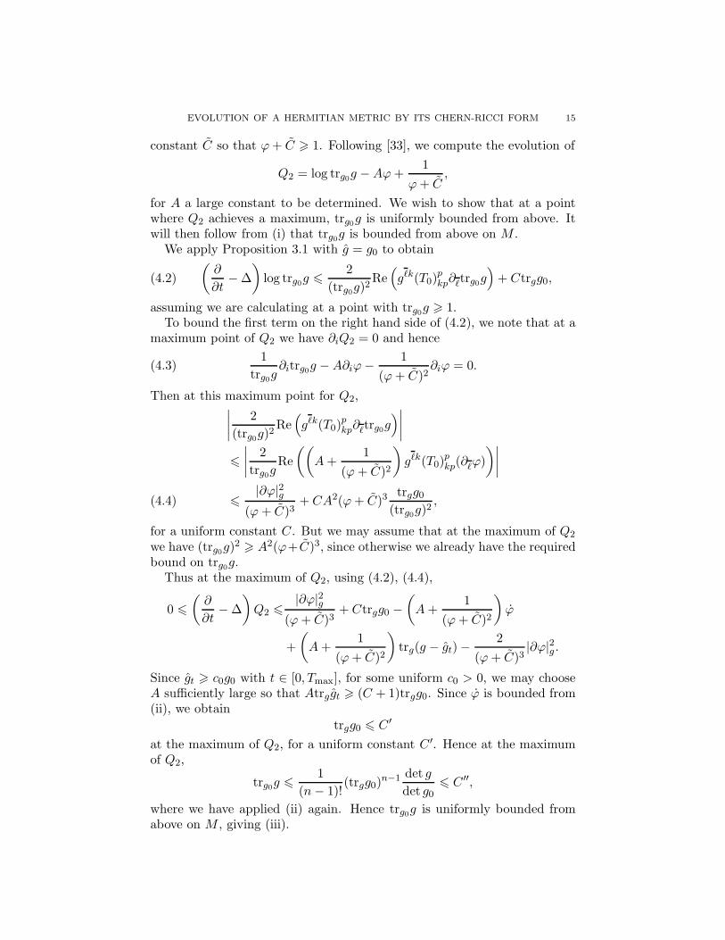
EVOLUTION OF A HERMITIAN METRIC BY ITS CHERN-RICCI FORM 15
constant C so that ϕ+ C > 1. Following [33], we compute the evolution of
Q2 = log trg0g −Aϕ+1
ϕ+ C,
for A a large constant to be determined. We wish to show that at a pointwhere Q2 achieves a maximum, trg0g is uniformly bounded from above. Itwill then follow from (i) that trg0g is bounded from above on M .
We apply Proposition 3.1 with g = g0 to obtain(
∂
∂t−∆
)
log trg0g 62
(trg0g)2Re(
gℓk(T0)pkp∂ℓtrg0g
)
+ Ctrgg0,(4.2)
assuming we are calculating at a point with trg0g > 1.To bound the first term on the right hand side of (4.2), we note that at a
maximum point of Q2 we have ∂iQ2 = 0 and hence
(4.3)1
trg0g∂itrg0g −A∂iϕ− 1
(ϕ+ C)2∂iϕ = 0.
Then at this maximum point for Q2,∣
∣
∣
∣
2
(trg0g)2Re(
gℓk(T0)pkp∂ℓtrg0g
)
∣
∣
∣
∣
6
∣
∣
∣
∣
2
trg0gRe
((
A+1
(ϕ+ C)2
)
gℓk(T0)pkp(∂ℓϕ)
)∣
∣
∣
∣
6|∂ϕ|2g
(ϕ + C)3+ CA2(ϕ+ C)3
trgg0(trg0g)
2,(4.4)
for a uniform constant C. But we may assume that at the maximum of Q2
we have (trg0g)2 > A2(ϕ+ C)3, since otherwise we already have the required
bound on trg0g.Thus at the maximum of Q2, using (4.2), (4.4),
0 6
(
∂
∂t−∆
)
Q2 6|∂ϕ|2g
(ϕ+ C)3+ Ctrgg0 −
(
A+1
(ϕ+ C)2
)
ϕ
+
(
A+1
(ϕ+ C)2
)
trg(g − gt)−2
(ϕ+ C)3|∂ϕ|2g .
Since gt > c0g0 with t ∈ [0, Tmax], for some uniform c0 > 0, we may chooseA sufficiently large so that Atrggt > (C + 1)trgg0. Since ϕ is bounded from(ii), we obtain
trgg0 6 C ′
at the maximum of Q2, for a uniform constant C ′. Hence at the maximumof Q2,
trg0g 61
(n− 1)!(trgg0)
n−1 det g
det g06 C ′′,
where we have applied (ii) again. Hence trg0g is uniformly bounded fromabove on M , giving (iii).
16 V. TOSATTI AND B. WEINKOVE
Part (iv) follows from the higher order estimates of Gill [19].
It is now straightforward to complete the proof of Theorem 1.2. We haveuniform estimates for the flow ϕ(t) on [0, Tmax). Taking limits we have asolution on [0, Tmax]. Applying the standard parabolic short time existencetheory we obtain a solution a little beyond Tmax, a contradiction. Hencethere exists a unique solution of (4.1) on [0, T0). Taking
√−1∂∂ of (4.1)
gives us a solution of (1.1) on [0, T0). Since T0 < T was chosen arbitrarily,we get a solution of (1.1) on [0, T ).
Uniqueness follows from uniqueness of solutions to (4.1). Clearly the flowcannot extend beyond T .
Next we give a proof of Theorem 1.3.
Proof of Theorem 1.3. Note that in general if ∂∂ω0 = 0 then ∂∂ω = 0 for alllater times. If n = 2 this means that the flow (1.1) preserves the Gauduchoncondition (recall that a Hermitian metric ω is Gauduchon if ∂∂ωn−1 = 0).The key result that we need is due to Buchdahl [7] and it says that if η is a∂∂-closed real (1, 1) form and ω0 a Gauduchon metric on a compact complexsurface M such that
∫
Mη2 > 0,
∫
Mη ∧ ω0 > 0,
∫
Dη > 0,
for all irreducible effective divisors D on M with D2 < 0, then there exists asmooth real function f such that η +
√−1∂∂f > 0 is a Gauduchon metric.
First of all observe that the following condition
(4.5)
∫
Mη2 > 0,
∫
Mη ∧ ω0 > 0,
∫
Dη > 0,
for all D as above is enough to guarantee the same conclusion. Indeedconsider the (1, 1) forms ηt = η + tω0, and take t > 0 large so that ηt is aGauduchon metric. Then we have
∫
Mη ∧ ηt =
∫
Mη2 + t
∫
Mη ∧ ω0 > 0,
and so we can apply Buchdahl’s result using ηt instead of ω0. In particular,if (4.5) holds then in fact we have the strict inequality
∫
M η ∧ ω0 > 0.We now apply this discussion to the (1, 1) forms αt = ω0 − tRic(ω0).
As we have seen earlier, the evolving metrics ω(t) are of the form ω(t) =αt +
√−1∂∂ϕt, and so it follows that T is the supremum of all t > 0 such
that
(4.6)
∫
Mα2t > 0,
∫
Mαt ∧ ω0 > 0,
∫
Dαt > 0,
for all D as above. Furthermore, if (4.6) holds at some time t then in fact∫
M αt ∧ ω0 > 0. Therefore T is also the supremum of all T0 > 0 such that∫
Mα2t > 0,
∫
Dαt > 0,
EVOLUTION OF A HERMITIAN METRIC BY ITS CHERN-RICCI FORM 17
hold for all t ∈ [0, T0].
5. Estimates away from a divisor
In this section we give the proof of Theorem 1.6. Let ω = ω(t) be thesolution of (1.1) on the maximal time interval [0, T ). We assume in thissection that T <∞.
In addition, we make the assumption that there exists a smooth functionfT on M such that
(5.1) ωT := αT +√−1∂∂fT > 0,
where we recall from (1.3) that αT = ω0−TRic(ω0). In the Kahler case (5.1)corresponds to the condition that the limiting Kahler class has a nonnegativerepresentative. Define reference metrics
ωt :=1
T((T − t)ω0 + tωT ) , for t ∈ [0, T ).
Then by the same argument as in the beginning of Section 4, we may writeω(t) = ωt +
√−1∂∂ϕ where ϕ = ϕ(t) solves the parabolic complex Monge-
Ampere equation
(5.2)∂
∂tϕ = log
(ωt +√−1∂∂ϕ)n
Ω, ωt +
√−1∂∂ϕ > 0, ϕ|t=0 = 0,
for the smooth volume form Ω = ωn0 e
fTT .
We begin with a proposition, which is exactly analogous to a result forthe Kahler-Ricci flow [50, 51] (see also the expositions in [37, 40]).
Proposition 5.1. With the assumptions above, there exists a constant Csuch that for all t ∈ [0, T ),
(i) ‖ϕ(t)‖C0 6 C.
(ii) ϕ(t) 6 C.
Proof. The proof is exactly the same as in the Kahler case. Briefly: theupper bound of ϕ follows from the same argument as in Lemma 4.1. For
the lower bound of ϕ observe that ωt =(T−t)
T ω0+tT ωT >
(T−t)T ω0 and hence
ωnt > c0(T − t)nΩ for a uniform c0 > 0. The lower bound of ϕ follows from
applying the maximum principle to the quantity
Q = ϕ+ n(T − t)(log(T − t)− 1)− (log c0 − 1)t.
Indeed if Q achieves its mimimum at some point (x, t) with t > 0 then at(x, t) we have
√−1∂∂ϕ > 0 and
0 >∂
∂tQ > log
ωnt
Ω− n log(T − t)− log c0 + 1 > 1,
a contradiction. Hence Q achieves its minimum at time t = 0 which givesthe lower bound for ϕ.
The upper bound of ϕ follows from the same argument as in Lemma4.1.
18 V. TOSATTI AND B. WEINKOVE
Next we prove a parabolic Schwarz lemma for volume forms for the flow(1.1). It holds in the special case that ωT is the pull-back of a metric fromanother Hermitian manifold via a holomorphic map. In the Kahler casethis is due to Song-Tian [34], and is a parabolic version of Yau’s (volume)Schwarz lemma [61].
Proposition 5.2. Let ω = ω(t) solve (1.1) on [0, T ) with T < ∞. Sup-pose we have a holomorphic map π : M → N for N a compact Hermitianmanifold of the same dimension n, equipped with a Hermitian metric ωN .Suppose that ωT = π∗ωN . Then there exists a uniform constant C > 0 suchthat on M × [0, T ),
ωn>
1
C(π∗ωN )n.
Proof. Call
u =(π∗ωN )n
ωn
the ratio of the volume forms. At any point where u > 0 we can calculate(
∂
∂t−∆
)
log u = trωπ∗Ric(ωN )− trωRic(ω)− gji
∂
∂tgij = trωπ
∗Ric(ωN ).
We apply the maximum principle to
Q = log u−Aϕ−An(T − t)(log(T − t)− 1),
for a constant A to be determined (cf. [40, Lemma 7.3]). The maximum ofQ is achieved at a point where u > 0, so we compute
(
∂
∂t−∆
)
Q = trωπ∗Ric(ωN )−Aϕ+An log(T − t) +Atrω(ω − ωt)
= −trω((A− 1)ωt − π∗Ric(ωN ))−A logωn
Ω(T − t)n
− trωωt +An.
Choose A sufficiently large so that for all t ∈ [0, T ],
(A−1)ωt−π∗Ric(ωN ) =(A− 1)
T((T − t)ω0 + tπ∗ωN )−π∗Ric(ωN ) > π∗ωN .
Note that by the arithmetic-geometric means inequality,
trωωt >(T − t)
Ttrωω0 > c
(
(T − t)nΩ
ωn
)1/n
,
for a uniform c > 0. Then(
∂
∂t−∆
)
Q 6 −trωπ∗ωN +A log
(T − t)nΩ
ωn− c
(
(T − t)nΩ
ωn
)1/n
+An
6 −trωπ∗ωN + C,
using the fact that the map x 7→ A log x− cx1/n is uniformly bounded fromabove for x > 0. Thus at a maximum point of Q we have trωπ
∗ωN 6 C, and
EVOLUTION OF A HERMITIAN METRIC BY ITS CHERN-RICCI FORM 19
applying the arithmetic-geometric means inequality again, u is uniformlybounded from above at this point. Since ϕ is uniformly bounded by Propo-sition 5.1, this implies that Q is bounded from above, and hence so is u.
Now assume that we are in the situation of Theorem 1.6. The map π :M → N is a holomorphic map blowing down an exceptional divisor E to apoint p ∈ N . More explicitly, a neighborhood of E in M can be identifiedwith
B = (z, ℓ) ∈ B × Pn−1 | z ∈ ℓ,
where B is the open unit ball in Cn and elements ℓ in P
n−1 are identifiedwith lines through the origin in C
n. The map π on B is identified with theprojection (z, ℓ) 7→ z ∈ B and the exceptional divisor E ⊂ M with the set
π−1(0) ⊂ B. π is a biholomorphism from M \E to N \ p.By assumption, there exists a function ψ = fT with
ωT := αT +√−1∂∂fT = π∗ωN .
Now there exists a Hermitian metric h on the fibers of the line bundle [E]associated to the divisor E with the property that for ε > 0 sufficientlysmall,
(5.3) π∗ωN − εRh > 0, with Rh = −√−1∂∂ log h.
For a proof of this statement, see [20, p. 187]. Although it is stated therein the Kahler case, the same proof carries over with ωN Hermitian. Fix s aholomorphic section of [E] vanishing along E to order 1.
We have a lemma:
Lemma 5.3. With these hypotheses, there exists A > 0 and C such that
trg0 g 6C
|s|2Ah.
Proof. Define, as in Tsuji’s work [56], ϕ = ϕ− ε0 log |s|2h, which is uniformlybounded from below and goes to infinity on E. Here ε0 > 0 is a smallconstant that will be specified below. Choose a constant C0 so that ϕ+C0 >
1. Following Phong-Sturm [33] (and as in Lemma 4.1 above), we computethe evolution of
Q = log trg0g −Aϕ+1
ϕ+ C0,
for A to be determined (assume at least Aε0 > 1). Note that the quantity1/(ϕ+C0) is bounded (in fact it lies between 0 and 1). Moreover, Q tends tonegative infinity on E and hence for each fixed time t, the quantity Q(x, t)achieves a maximum at some point in M \E.
From Proposition 3.1 we have(
∂
∂t−∆
)
log trg0g 62
(trg0g)2Re(
gℓk(T0)pkp∂ℓtrg0g
)
+ Ctrgg0,(5.4)
20 V. TOSATTI AND B. WEINKOVE
assuming we are calculating at a point with trg0g > 1. To bound the firstterm on the right hand side, we note that at a maximum point of Q we have∂iQ = 0 and hence
1
trg0g∂itrg0g −A∂iϕ− 1
(ϕ+ C0)2∂iϕ = 0.
Thus at this maximum point for Q,∣
∣
∣
∣
2
(trg0g)2Re(
gℓk(T0)pkp∂ℓtrg0g
)
∣
∣
∣
∣
6
∣
∣
∣
∣
2
trg0gRe
((
A+1
(ϕ+ C0)2
)
gℓk(T0)pkp(∂ℓϕ)
)∣
∣
∣
∣
6|∂ϕ|2g
(ϕ+ C0)3+ CA2(ϕ+ C0)
3 trgg0(trg0g)
2,
for a uniform constant C. If at the maximum of Q we have (trg0g)2 6
A2(ϕ+ C0)3 then at the same point we have
(trg0g)|s|2Aε0h 6 A(ϕ− ε0 log |s|2h + C0)
3
2 |s|2Aε0h 6 CA,
for a constant CA depending on A, and so
Q = log((trg0g)|s|2Aε0h )−Aϕ+
1
ϕ+ C06 C ′
A,
and we are done. If on the other hand at the maximum of Q we haveA2(ϕ+ C0)
3 6 (trg0g)2 then
∣
∣
∣
∣
2
(trg0g)2Re(
gℓk(T0)pkp∇ℓtrg0g
)
∣
∣
∣
∣
6|∂ϕ|2g
(ϕ+ C0)3+ Ctrgg0.
Now compute at the maximum of Q, using (5.4)
0 6
(
∂
∂t−∆
)
Q 6|∂ϕ|2g
(ϕ+ C0)3+ Ctrgg0 −
(
A+1
(ϕ+ C0)2
)
ϕ
+
(
A+1
(ϕ+ C0)2
)
trω(ω − (ωt − ε0Rh))
− 2
(ϕ+ C0)3|∂ϕ|2g.(5.5)
Since we clearly have ωt > cωT for some constant c > 0, we can use (5.3) toget that ωt − ε0Rh > c0ω0 for some uniform c0 > 0, provided we choose ε0sufficiently small. Hence we may choose A sufficiently large so that
trgg0 6 C logΩ
ωn+ C.
Hence at the maximum of Q,
trg0g 61
(n− 1)!(trgg0)
n−1 det g
det g06 C
ωn
Ω
(
logΩ
ωn
)n−1
+ C 6 C ′,
EVOLUTION OF A HERMITIAN METRIC BY ITS CHERN-RICCI FORM 21
because we know that ωn
Ω 6 C and x 7→ x| log x|n−1 is bounded above for xclose to zero. This implies that Q is bounded from above at its maximum,and completes the proof of the lemma.
It is now straightforward to complete the proof of the theorem.
Proof of Theorem 1.6. We apply Proposition 5.2 and Lemma 5.3 to see thatfor any compact set K ⊂M \ E, there exists a constant CK > 0 such that
C−1K ω0 6 ω(t) 6 CKω0 on K × [0, T ).
Applying the higher order estimates of Gill [19], which are local, we obtainuniform C∞ estimates for ω(t) on compact subsets of M \E. In particular,for every compact set K there exists a constant C ′
K such that
∂
∂tω = −Ric(ω) 6 C ′
Kω,
which implies that e−C′K tω(t) is decreasing in t as well as being bounded
from below. This implies that a limit for ω(t) exists as t→ T , and since wehave uniform estimates away from E, we see that ω(t) converges in C∞ oncompact subsets to a smooth Hermitian metric ωT on M \E.
6. The Chern-Ricci flow on complex surfaces
In this section we give a proof of Theorem 1.5, and we pose some conjec-tures on the behavior of the Chern-Ricci flow on surfaces, and its relationto the ‘minimal model program for complex surfaces’.
First recall that the Kodaira dimension of a compact complex manifoldM of dimension n is given by
κ(M) = lim supℓ→+∞
log dimH0(M, ℓKM )
log ℓ∈ −∞, 0, 1, . . . , n.
Proof of Theorem 1.5. (a) We need to show that if T = ∞ then M is min-imal. If M is a non-minimal compact complex surface then we must haveT <∞, because if D is any (−1)-curve in M we have that D ·KM < 0 andso the volume of D,
∫
Dω(t) =
∫
Dω0 + 2πtD ·KM ,
becomes zero in finite time.(b) If the volume goes to zero at time T < ∞, we have that
∫
M α2T =
0, where we recall from (1.3) that αT is the ∂∂-closed (1, 1) form αT =ω0 − TRic(ω0). We claim that in this case the Kodaira dimension κ(M) isnegative, which by the Kodaira-Enriques classification [2, 3] implies that Mis either birational to a ruled surface or of class VII. Indeed, if κ(M) > 0then some power ℓKM , ℓ > 1 of the canonical bundle would be effective. LetE be an effective divisor in |ℓKM |, then E must be nonempty since otherwiseℓKM would be trivial, and so cBC
1 (M) = 0 and by Theorem 1.1 we wouldhave T = ∞. We thus conclude that E is nonempty, and let s be a section
22 V. TOSATTI AND B. WEINKOVE
of ℓKM defining E and h a smooth metric on the fibers of ℓKM . Then bythe Poincare-Lelong formula the curvature η of h is a smooth closed real(1, 1) form such that
2π[E] = η +√−1∂∂ log |s|2h
holds as currents onM (see also [17]). In particular for any ∂∂-closed smooth(1, 1) form γ we have
∫
Mγ ∧ η = 2π
∫
Eγ.
Moreover if γ is a Gauduchon metric we have∫
Mγ ∧ cBC
1 (M) = −2π
ℓ
∫
Eγ < 0,
because −1ℓη represents cBC
1 (M). Taking γ = ω(t) and letting t approach Twe get
∫
MαT ∧ cBC
1 (M) 6 0.
We also have
0 =
∫
Mα2T = −T
∫
MαT ∧ cBC
1 (M) +
∫
MαT ∧ ω0
>
∫
MαT ∧ ω0 > 0,
which implies that∫
M αT ∧ω0 = 0. Applying [6, Lemma 4] we see that αT =√−1∂∂f for some smooth function f , which implies that ω0 is Kahler and
thatM is Fano, contradicting the assumption that the Kodaira dimension ofM is nonnegative. To see that M cannot be an Inoue surface, we apply theobservation (below) that on an Inoue surface, the Chern-Ricci flow existsfor all time.
(c) Assume now that T < ∞ and that the volume does not collapse attime T , so that
∫
M α2T > 0. We know from Theorem 1.2 that there is no
smooth function f such that αT +√−1∂∂f > 0 (otherwise we could continue
the flow past T ). On the other hand for ε > 0
αT + εω0 = (1 + ε)ω0 − TRic(ω0) = (1 + ε)
(
ω0 −T
1 + εRic(ω0)
)
,
and since T1+ε < T we have ω0− T
1+εRic(ω0)+√−1∂∂f > 0 for some function
f . Therefore∫
Mω0 ∧ (αT + εω0) > 0,
and letting ε→ 0 we get∫
M αT ∧ ω0 > 0, therefore∫
MαT ∧ (αT + εω0) =
∫
Mα2T + ε
∫
MαT ∧ ω0 > 0.
EVOLUTION OF A HERMITIAN METRIC BY ITS CHERN-RICCI FORM 23
We now apply the main theorem of [7], and we see that there is an irreducibleeffective divisor D ⊂M with D2 < 0 such that
∫
D αT = 0. Furthermore
(6.1) 2πKM ·D = −∫
DRic(ω0) =
1
T
∫
D(αT − ω0) = − 1
T
∫
Dω0 < 0,
and so by the adjunction formula D is a smooth (−1)-curve.Assume now that M is minimal and consider first the case when M is
Kahler. If κ(M) > 0 then KM is nef thanks to [2, Corollary III.2.4], while ifκ(M) = −∞ then by the Kodaira-Enriques classification M is either CP2 orruled. If KM is nef then
∫
M cBC1 (M)2 > 0 and if κ(M) > 0 then some power
of KM is effective, so the argument above implies that∫
M ω0∧ cBC1 (M) < 0.
Thus the volume along the flow is
Vt =
∫
Mω(t)2 =
∫
Mω20 − 2t
∫
Mω0 ∧ cBC
1 (M) + t2∫
McBC1 (M)2,
which is always positive, so by Theorem 1.3 we have T = ∞. On the otherhand if M is CP2 or ruled then we must have T < ∞ and since case (c) isexcluded we must be in case (b). Indeed, if M is CP2 and E is a line insideit then E ·KM < 0 and its volume
∫
Eω(t) =
∫
Eω0 + 2πtE ·KM
goes to zero in finite time. The other case is when M is ruled and E ∼= CP1
is a fiber of the ruling then E ·E = 0 and by the genus formula E ·KM = −2,which again implies that the volume of E goes to zero in finite time.
If on the other hand M is not Kahler, thanks to the Kodaira-Enriquesclassification [2, 3] we know that minimal non-Kahler compact complex sur-faces fall into the following classes:
(1) Primary and secondary Kodaira surfaces,(2) Surfaces of class VII with b2(M) = 0,(3) Minimal surfaces of class VII with b2(M) > 0,(4) Minimal properly elliptic surfaces,
where a surface of class VII is by definition a compact complex surface withb1(M) = 1 and κ(M) = −∞, while a properly elliptic surface is an ellipticsurface with κ(M) = 1. The surfaces in (1), (2) and (4) are completelyclassified, and while there are many examples of surfaces in (3), a completeclassification is still lacking (see e.g. [2, 13, 27, 29, 46, 47, 49]). We treateach case separately.
In case (1) the manifold M has torsion canonical bundle (i.e. some powerℓKM , ℓ > 1 is holomorphically trivial). In particular these manifolds havecBC1 (M) = 0, and Theorem 1.1 says that the Chern-Ricci flow starting fromany initial Hermitian metric ω0 has a long time solution ω(t) (so we arein case (a)) which as t goes to infinity converges smoothly to the uniqueHermitian metric of the form ω∞ = ω0 +
√−1∂∂ϕ∞ with Ric(ω∞) = 0.
24 V. TOSATTI AND B. WEINKOVE
In case (2), the manifold M is either an Inoue surface or a Hopf surface[27, 46]. Suppose first that M is an Inoue surface. Then M does nothave any curves and by [48, Remark 4.2] any Gauduchon metric ω0 satisfies∫
M ω0 ∧ cBC1 (M) < 0. In particular the volume of M along the flow is
Vt =
∫
Mω(t)2 =
∫
Mω20 − 2t
∫
Mω0 ∧ cBC
1 (M).
Since Vt is always positive, Theorem 1.3 implies that the Chern-Ricci flowexists for all positive time, so we are in case (a).
If M is a Hopf surface, it follows from the arguments in [48, Remark 4.3]that any Gauduchon metric ω0 on them satisfies
∫
M ω0∧cBC1 (M) > 0. Indeed
as we have seen this holds wheneverM has a plurianticanonical divisor, and[48, Remark 4.3] shows that every primary Hopf surface has an anticanonicaldivisor. But every Hopf surface is either primary or secondary (i.e. a finite
unramified quotient M →M of a primary one) and an anticanonical divisor
on M gives a plurianticanonical divisor on M . In particular the volume ofM along the flow is
Vt =
∫
Mω(t)2 =
∫
Mω20 − 2t
∫
Mω0 ∧ cBC
1 (M),
which goes to zero in finite time, and so the Chern-Ricci flow exists for finitetime. In fact, since every curve on M is homologous to zero, the flow existsprecisely as long as the volume stays positive and then it collapses, so weare in case (b). We will investigate the behavior of the flow on a family ofHopf manifolds in Section 8.
In case (3), if we call b2(M) = n > 0, we have∫
M c21(M) = −n (see e.g.[47, p.494]). It follows that the Chern-Ricci flow starting from any initialGauduchon metric ω0 exists only for finite time, because the volume of Malong the flow is
Vt =
∫
Mω(t)2 =
∫
Mω20 − 2t
∫
Mω0 ∧ cBC
1 (M)− 4π2nt2,
which goes to zero in finite time. Furthermore, sinceM is minimal and usingagain Theorem 1.3, we see that we are in case (b). Note that carrying outa space-time rescaling of the flow to have constant volume will still producea solution that exists only for a finite time (cf. the discussion in [44]).
In case (4) we have∫
M c21(M) = 0 and by definition some power of thecanonical bundle ℓKM , ℓ > 1, is effective. Arguing as before, this impliesthat
∫
Mω0 ∧ cBC
1 (M) < 0.
Therefore the volume along the Chern-Ricci flow remains positive for alltime, and since M is minimal the flow has a long time solution and we arein case (a).
EVOLUTION OF A HERMITIAN METRIC BY ITS CHERN-RICCI FORM 25
Furthermore, arguing like in [40, Proposition 8.4], one can show that incase (b) the volume goes to zero quadratically only on a Fano manifold in apositive multiple of the anticanonical class, otherwise it goes to zero linearly.
We finish this section with some further discussions and conjectures. Webegin by considering what happens in case (c), along the lines of [40, The-orem 8.3]. First of all note that αT is a ∂∂-closed real (1, 1) form with∫
M α2T > 0. It follows from [6, Lemma 4] that if ψ is another ∂∂-closed real
(1, 1) form with∫
M ψ ∧ αT = 0 then∫
M ψ2 6 0 with equality if and only
if ψ =√−1∂∂f for some function f . If now D1,D2 are irreducible distinct
(−1)-curves (so D1 ·D2 > 0) with∫
D1αT =
∫
D2αT = 0, then as before we
can express the divisor D1 +D2 as
2π[D1 +D2] = η +√−1∂∂ log |s|2h,
in the sense of currents, where η is a smooth closed form that represents2πc1(D1 +D2). Therefore, since ∂∂αT = 0,
0 =
∫
D1
αT +
∫
D2
αT =1
2π
∫
Mη ∧ αT ,
and so 4π2(D1 + D2)2 =
∫
M η2 6 0, with equality implying that η =√−1∂∂f . But this would give
0 = −∫
Mη ∧ cBC
1 (M) = 2πKM · (D1 +D2) < 0,
a contradiction. Thus we conclude that (D1 +D2)2 < 0, which implies that
D1 ·D2 = 0 and D1,D2 are disjoint. The set of all these (−1)-curves is finite,D1, . . . ,Dk say, because they give linearly independent classes in homology.Contracting all of them we get a contraction map π : M → N , where N isa compact complex surface which is Kahler if and only if M is.
In light of the behavior of the Kahler-Ricci flow on surfaces, it is naturalto ask whether the Chern-Ricci flow contracts, in the sense of [38], the(−1)-curves D1, . . . ,Dk to points p1, . . . , pk on N . First, do the metrics ω(t)converge smoothly on compact subsets of M \ ⋃iDi to a smooth Kahlermetric ω(T ) on M \ ⋃iDi, as in Theorem 1.6? This would hold if we can
find β, a ∂∂-closed real (1, 1) form on N , and f a smooth function on Msuch that π∗β = αT +
√−1∂∂f .
Furthermore, does the family (M,ω(t)) converge in the sense of Gromov-Hausdorff to a limiting compact metric space (N, d) as t → T−? Can weproduce a solution of the Chern-Ricci flow ω(t) on N for t ∈ [T, T ′] (withT ′ > T ) such that ω(T ) on N \ p1, . . . , pk can be identified with ω(T ) viathe blow-down map? Does the family (N, ω(t)) converge in the Gromov-Hausdorff sense to (N, d) as t→ T+?
If this can be carried out, one could continue this process a finite numberof times to obtain a solution of the Chern-Ricci flow ‘with canonical surgicalcontractions’ [38] all the way to the minimal model of M .
26 V. TOSATTI AND B. WEINKOVE
Finally, what is the long time behavior of the Chern-Ricci flow on a min-imal model M? In the case when M has Kodaira dimension zero, so that ithas torsion canonical bundle (and is either a Calabi-Yau surface or a Kodairasurface) the flow always converges to a Chern-Ricci flat metric (which neednot be Kahler, even if M is Calabi-Yau) by Gill’s Theorem 1.1. Anothercase (of course there are many more) is when c1(M) < 0. We discuss thiscase, for any dimension, in the next section.
7. Convergence when c1(M) < 0
In this section we assume that M is a compact Kahler manifold withc1(M) < 0 and we give the proof of Theorem 1.7.
Start by fixing a smooth volume form Ω with Ric(Ω) < 0, which is possiblebecause c1(M) < 0, and note that Ric(Ω) also represents cBC
1 (M). There-fore, for all t > 0 the (1, 1) form ω0 − tRic(Ω) is positive, and by Theorem1.2 the Chern-Ricci flow (1.1) exists for all time. Call ω(s) its solution.
We consider now the rescaled metrics ω = ωs+1 and a new time parameter
t = log(s+ 1), so that the new metrics solve
(7.1)∂
∂tω = −Ric(ω)− ω, ω|t=0 = ω0,
for all positive t. First of all we show that (7.1) is equivalent to a para-bolic complex Monge-Ampere equation. To see this, call ω = −Ric(Ω) +e−t(Ric(Ω) + ω0), and note that they are Hermitian metrics that satisfy
(7.2)∂
∂tω = −Ric(Ω)− ω, ω|t=0 = ω0,
and ω converges smoothly to −Ric(Ω) as t goes to infinity. It follows that
∂
∂t(ω − ω) = −(ω − ω) +
√−1∂∂ log
ωn
Ω.
Consider now the solution ϕ of the equation
(7.3)∂
∂tϕ = log
ωn
Ω− ϕ, ϕ|t=0 = 0,
which exists for all positive time as can be seen by regarding it as an ODEin t for each fixed point on M . We have that
∂
∂t
(
et(ω − ω −√−1∂∂ϕ)
)
= 0, (ω − ω −√−1∂∂ϕ)|t=0 = 0,
which implies that ω = ω +√−1∂∂ϕ holds for t > 0. Then Theorem 1.7
follows directly from:
Theorem 7.1. As t → ∞ we have that ϕ → ϕ∞ smoothly, and ω∞ :=−Ric(Ω) +
√−1∂∂ϕ∞ equals the unique Kahler-Einstein metric ωKE.
Proof. First, we derive uniform estimates for ϕ independent of t. The esti-mates for ‖ϕ‖C0 and ‖ϕ‖C0 follow from the same arguments as in [8, 51, 56].
EVOLUTION OF A HERMITIAN METRIC BY ITS CHERN-RICCI FORM 27
Indeed, a simple maximum principle argument shows that |ϕ| 6 C indepen-dent of t. Compute
(
∂
∂t−∆
)
ϕ = −ϕ− trω(Ric(Ω) + ω)
= −ϕ− n+∆ϕ− trωRic(Ω),
and so(
∂
∂t−∆
)
(ϕ+ ϕ) = −n− trωRic(Ω).
At the minimum of ϕ+ϕ, assuming it occurs for t > 0, we have−trωRic(Ω) 6n, and since Ric(Ω) < 0 the arithmetic-geometric means inequality gives usϕ + ϕ = log ωn
Ω > −C at this point and hence everywhere. Since |ϕ| 6 C,we get ϕ > −C. But we also have that Ric(Ω) + ω = e−t(Ric(Ω) + ω0), andso
(
∂
∂t−∆
)
(ϕ+ ϕ+ nt− etϕ) = trωω0 > 0,
which implies by the maximum principle that, for t > 1, ϕ 6 Cte−t 6
Ce−t/2. This estimate is the same as the one in [51].We feed this into the second order estimate as before. We have(
∂
∂t−∆
)
log trg0g 62e−t
(trg0g)2Re(
gℓk(T0)pkp∂ℓtrg0g
)
+ Ctrgg0 − 1,
assuming we are calculating at a point with trg0g > 1. Indeed, this followsfrom the calculations of Proposition 3.1 with g = g0, with the minor changethat now g(t) evolves by the normalized Chern-Ricci flow. In particular, wenow have dω = e−tdω0 instead of dω = dω0.
Arguing as in the proof of Lemma 4.1 we get that ω is uniformly equivalentto ω0 independent of t. Uniform higher order estimates are then providedby Gill’s paper [19]. In particular, it follows that
(
∂
∂t−∆
)
(etϕ) = −trω(Ric(Ω) + ω0) > −C,
and so the maximum principle implies that ϕ > −C(1 + t)e−t > −Ce−t/2.This implies that as t approaches infinity ϕ converges uniformly to zeroexponentially fast, which implies that ϕ converges uniformly exponentiallyfast to a continuous limit function ϕ∞. Since we have uniform higher orderestimates for ϕ, it follows that ϕ∞ is actually smooth and the convergenceof ϕ to ϕ∞ is in the smooth topology. Therefore we can pass to the limit in(7.3) and see that the limiting metric ω∞ = −Ric(Ω) +
√−1∂∂ϕ∞ satisfies
logωn∞
Ω= ϕ∞,
and taking√−1∂∂ of this, we get
Ric(ω∞) = −ω∞,
so that ω∞ is the unique Kahler-Einstein metric on M .
28 V. TOSATTI AND B. WEINKOVE
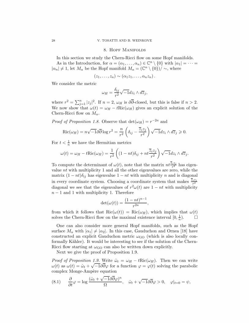
8. Hopf Manifolds
In this section we study the Chern-Ricci flow on some Hopf manifolds.As in the Introduction, for α = (α1, . . . , αn) ∈ C
n \ 0 with |α1| = · · · =|αn| 6= 1, let Mα be the Hopf manifold Mα = (Cn \ 0)/ ∼, where
(z1, . . . , zn) ∼ (α1z1, . . . , αnzn) .
We consider the metric
ωH =δijr2
√−1dzi ∧ dzj ,
where r2 =∑n
j=1 |zj |2. If n = 2, ωH is ∂∂-closed, but this is false if n > 2.
We now show that ω(t) = ωH − tRic(ωH) gives an explicit solution of theChern-Ricci flow on Mα.
Proof of Proposition 1.8. Observe that det(ωH) = r−2n and
Ric(ωH) = n√−1∂∂ log r2 =
n
r2
(
δij −zizjr2
)√−1dzi ∧ dzj > 0.
For t < 1n we have the Hermitian metrics
ω(t) = ωH − tRic(ωH) =1
r2
(
(1− nt)δij + ntzizjr2
)√−1dzi ∧ dzj.
To compute the determinant of ω(t), note that the matrix ntzizjr2 has eigen-
value nt with multiplicity 1 and all the other eigenvalues are zero, while thematrix (1− nt)δij has eigenvalue 1− nt with multiplicity n and is diagonal
in every coordinate system. Choosing a coordinate system that makeszizjr2
diagonal we see that the eigenvalues of r2ω(t) are 1 − nt with multiplicityn− 1 and 1 with multiplicity 1. Therefore
det(ω(t)) =(1− nt)n−1
r2n,
from which it follows that Ric(ω(t)) = Ric(ωH), which implies that ω(t)solves the Chern-Ricci flow on the maximal existence interval [0, 1n).
One can also consider more general Hopf manifolds, such as the Hopfsurface Mα with |α1| 6= |α2|. In this case, Gauduchon and Ornea [18] haveconstructed an explicit Gauduchon metric ωGO (which is also locally con-formally Kahler). It would be interesting to see if the solution of the Chern-Ricci flow starting at ωGO can also be written down explicitly.
Next we give the proof of Proposition 1.9.
Proof of Proposition 1.9. Write ωt = ωH − tRic(ωH). Then we can writeω(t) as ω(t) = ωt +
√−1∂∂ϕ for a function ϕ = ϕ(t) solving the parabolic
complex Monge-Ampere equation
(8.1)∂
∂tϕ = log
(ωt +√−1∂∂ϕ)n
Ω, ωt +
√−1∂∂ϕ > 0, ϕ|t=0 = ψ,
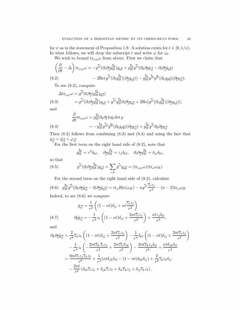
EVOLUTION OF A HERMITIAN METRIC BY ITS CHERN-RICCI FORM 29
for ψ as in the statement of Proposition 1.9. A solution exists for t ∈ [0, 1/n).In what follows, we will drop the subscript t and write ω for ωt.
We wish to bound trωHω from above. First we claim that
(
∂
∂t−∆
)
trωHω = −gji(∂i∂jgℓkH )gkℓ + gℓkH g
ji(∂k∂ℓgij − ∂i∂j gkℓ)
− 2Re(gji(∂igℓkH )(∂jgkℓ))− gℓkH g
jpgqi(∂kgpq)(∂ℓgij).(8.2)
To see (8.2), compute
∆trωHω = gji∂i∂j(g
ℓkH gkℓ)
= gji(∂i∂jgℓkH )gkℓ + gjigℓkH ∂i∂jgkℓ + 2Re(gji(∂ig
ℓkH )(∂jgkℓ)),(8.3)
and∂
∂ttrωH
ω = gℓkH ∂k∂ℓ log det g
= −gℓkH gjpgqi(∂kgpq)(∂ℓgij) + gℓkH gji∂k∂ℓgij .(8.4)
Then (8.2) follows from combining (8.3) and (8.4) and using the fact thatgij = gij + ϕij .
For the first term on the right hand side of (8.2), note that
gℓkH = r2δkℓ, ∂jgℓkH = zjδkℓ, ∂i∂jg
ℓkH = δijδkℓ,
so that
(8.5) gji(∂i∂jgℓkH )gkℓ =
∑
i,k
giigkk = (trωHω)(trωωH).
For the second term on the right hand side of (8.2), calculate
(8.6) gℓkH gji(∂k∂ℓgij − ∂i∂j gkℓ) = trωRic(ωH)− ngji
zizjr4
− (n− 2)trωωH .
Indeed, to see (8.6) we compute
gij =1
r2
(
(1− nt)δij + ntzizjr2
)
∂ℓgij = − 1
r4zℓ
(
(1− nt)δij +2ntzizjr2
)
+ntzjδiℓr4
,(8.7)
and
∂k∂ℓgij =2
r6zkzℓ
(
(1− nt)δij +2ntzizjr2
)
− 1
r4δkℓ
(
(1− nt)δij +2ntzizjr2
)
− 1
r4zℓ
(
−2ntzk zizjr4
+2ntziδjk
r2
)
− 2ntzkzjδiℓr6
+ntδjkδiℓr4
=6ntzizjzkzℓ
r8+
1
r4(ntδjkδiℓ − (1− nt)δkℓδij) +
2
r6zkzℓδij
− 2nt
r6(δkℓzizj + δjkzizℓ + δiℓzkzj + δijzkzℓ) ,
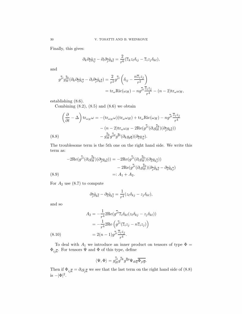
30 V. TOSATTI AND B. WEINKOVE
Finally, this gives:
∂k∂ℓgij − ∂i∂j gkℓ =2
r6(zkzℓδij − zizjδkℓ),
and
gjigℓkH (∂k∂ℓgij − ∂i∂j gkℓ) =2
r2gji(
δij −nzizjr2
)
= trωRic(ωH)− ngjizizjr4
− (n− 2)trωωH ,
establishing (8.6).Combining (8.2), (8.5) and (8.6) we obtain
(
∂
∂t−∆
)
trωHω = −(trωH
ω)(trωωH) + trωRic(ωH)− ngjizizjr4
− (n− 2)trωωH − 2Re(gji(∂igℓkH )(∂jgkℓ))
− gℓkH gjpgqi(∂kgpq)(∂ℓgij).(8.8)
The troublesome term is the 5th one on the right hand side. We write thisterm as:
−2Re(gji(∂igℓkH )(∂jgkℓ)) = −2Re(gji(∂ig
ℓkH )(∂ℓgkj))
− 2Re(gji(∂igℓkH )(∂j gkℓ − ∂ℓgkj)
=: A1 +A2.(8.9)
For A2 use (8.7) to compute
∂j gkℓ − ∂ℓgkj =1
r4(zℓδkj − zjδkℓ),
and so
A2 = − 1
r42Re(gjiziδkℓ(zℓδkj − zjδkℓ))
= − 1
r42Re
(
gji(zizj − nzizj))
= 2(n− 1)gjizizjr4
.(8.10)
To deal with A1 we introduce an inner product on tensors of type Φ =Φijk. For tensors Ψ and Φ of this type, define
〈Ψ,Φ〉 = gjiHgℓkgqpΨikqΦjℓp.
Then if Φijk = ∂igjk we see that the last term on the right hand side of (8.8)
is −|Φ|2.
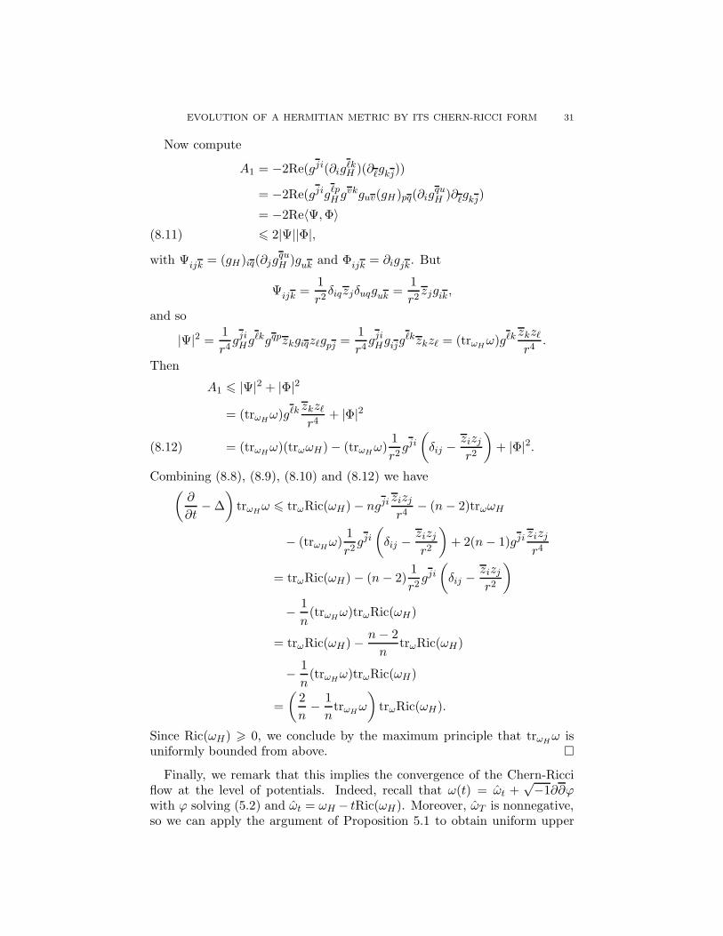
EVOLUTION OF A HERMITIAN METRIC BY ITS CHERN-RICCI FORM 31
Now compute
A1 = −2Re(gji(∂igℓkH )(∂ℓgkj))
= −2Re(gjigℓpH gvkguv(gH)pq(∂ig
quH )∂ℓgkj)
= −2Re〈Ψ,Φ〉6 2|Ψ||Φ|,(8.11)
with Ψijk = (gH)iq(∂jgquH )guk and Φijk = ∂igjk. But
Ψijk =1
r2δiqzjδuqguk =
1
r2zjgik,
and so
|Ψ|2 = 1
r4gjiHg
ℓkgqpzkgiqzℓgpj =1
r4gjiHgijg
ℓkzkzℓ = (trωHω)gℓk
zkzℓr4
.
Then
A1 6 |Ψ|2 + |Φ|2
= (trωHω)gℓk
zkzℓr4
+ |Φ|2
= (trωHω)(trωωH)− (trωH
ω)1
r2gji(
δij −zizjr2
)
+ |Φ|2.(8.12)
Combining (8.8), (8.9), (8.10) and (8.12) we have(
∂
∂t−∆
)
trωHω 6 trωRic(ωH)− ngji
zizjr4
− (n− 2)trωωH
− (trωHω)
1
r2gji(
δij −zizjr2
)
+ 2(n− 1)gjizizjr4
= trωRic(ωH)− (n− 2)1
r2gji(
δij −zizjr2
)
− 1
n(trωH
ω)trωRic(ωH)
= trωRic(ωH)− n− 2
ntrωRic(ωH)
− 1
n(trωH
ω)trωRic(ωH)
=
(
2
n− 1
ntrωH
ω
)
trωRic(ωH).
Since Ric(ωH) > 0, we conclude by the maximum principle that trωHω is
uniformly bounded from above.
Finally, we remark that this implies the convergence of the Chern-Ricciflow at the level of potentials. Indeed, recall that ω(t) = ωt +
√−1∂∂ϕ
with ϕ solving (5.2) and ωt = ωH − tRic(ωH). Moreover, ωT is nonnegative,so we can apply the argument of Proposition 5.1 to obtain uniform upper
32 V. TOSATTI AND B. WEINKOVE
bounds for |ϕ| and ϕ. It follows immediately that as t→ T , ϕ(t) convergespointwise to a function ϕ(T ) on Mα. On the other hand, by Proposition 1.9we have uniform bounds for |∆gHϕ|. Thus standard elliptic theory gives auniform bound for ‖ϕ(t)‖C1+β for any β ∈ (0, 1). It follows that ϕ → ϕ(T )in C1+β for any β ∈ (0, 1).
9. The complex Monge-Ampere equation
In this section we prove uniform estimates for solutions of the ellipticcomplex Monge-Ampere equation.
Let (Mn, ω) be a compact Hermitian manifold, F a smooth function onM and ω′ = ω +
√−1∂∂ϕ a Hermitian metric that satisfies
(9.1) (ω +√−1∂∂ϕ)n = eFωn.
We will give an alternative proof of the main result of [54] (see also [4, 12]for different proofs):
Theorem 9.1. There is a constant C that depends only on (M,ω), supM Fand infM ∆F such that
(9.2) supM
ϕ− infMϕ 6 C.
This is slightly weaker than the result in [54], because there is no depen-dence of C on infM ∆F there (and in fact the proof of [54] can be easilymodified to have C depend only on p > n and
∫
M epF rather than supM F ).The point of our discussion here is to establish Theorem 9.1 via a new secondorder estimate which we had previously established [53] using the maximumprinciple only in the cases n = 2 or (M,ω) balanced.
From now on we will normalize ϕ by assuming supM ϕ = 0. The estimatewe wish to prove is:
(9.3) trgg′ 6 CeA(ϕ−infM ϕ)
for uniform constants C,A. The reader may notice that (9.3) has the sameform as the second order estimates of Yau and Aubin [1, 60].
Theorem 9.1 then follows from (9.3). Indeed, we can then use the argu-ments in [53] to derive (9.2) from (9.3). The idea is that a second orderestimate of the form (9.3), together with the condition
√−1∂∂ϕ > −ω im-
plies, via a Moser iteration argument applied to the exponential of ϕ, a zeroorder estimate for ϕ. This method was employed in the Kahler case in [59],and a related argument was used in the almost complex setting in [55].
Proof of (9.3). Following Phong-Sturm [33] we consider the quantity
Q = log trgg′ −Aϕ+
1
ϕ− infM ϕ+ 1,
EVOLUTION OF A HERMITIAN METRIC BY ITS CHERN-RICCI FORM 33
for A > 1 to be determined. Note that 0 < 1ϕ−infM ϕ+1 6 1. We have
∆′Q = ∆′ log trgg′ −An+Atrg′g −
n− trg′g
(ϕ− infM ϕ+ 1)2
+2|∂ϕ|2g′
(ϕ− infM ϕ+ 1)3
> ∆′ log trgg′ +Atrg′g +
2|∂ϕ|2g′(ϕ− infM ϕ+ 1)3
−An− n,
(9.4)
writing ∆′ for the complex Laplacian associated to g′. To calculate ∆′ log trgg′
we go back to the calculations in Proposition 3.1 where g = g0 is now re-placed by g and g′ takes the role of the evolving metric there. With thesesubstitutions (3.3), (3.4) and (3.6) together read
∆′trgg′ = g′jigℓk∇ℓ∇kg
′
ij+ g′ji∇iT ℓ
jℓ + g′jigℓkgpj∇ℓTpik
− g′jigℓkg′kq(∇iTqjℓ −Riℓpjg
qp)
−R− 2Re(
g′jigℓkT pik∇ℓg
′
pj
)
− g′jigℓkT pikT
qjℓgpq + g′jigℓkT p
ikTqjℓg
′
pq,
where R = gℓkRCkℓ
= gjigℓkRkℓij is the Chern scalar curvature of g. On the
other hand by applying ∆ log to (9.1) we get
∆F −R = gℓk∂k∂ℓ log det(g′) = g′jigℓk∂k∂ℓg
′
ij− g′jpg′qigℓk∂kg
′
ij∂ℓg
′
pq,
and converting these into covariant derivatives (as in the argument for (3.5)in the proof of Proposition 3.1) we get
∆F = g′jigℓk∇ℓ∇kg′
ij− g′jpg′qigℓk∇kg
′
ij∇ℓg
′
pq,
and so
∆′ log trgg′ =
1
trgg′
(
[
g′jpg′qigℓk∇kg′
ij∇ℓg
′
pq −1
trgg′g′ℓk∇ktrgg
′∇ℓtrgg′
+ 2Re(
g′jigℓkT pki∇ℓg
′
pj
)
+ g′jigℓkT pikT
qjℓg
′
pq
]
+∆F −R
+ g′ji∇iTℓjℓ + g′jigℓkgpj∇ℓT
pik − g′jigℓkg′kq(∇iT
qjℓ −Riℓpjg
qp)
− g′jigℓkT pikT
qjℓgpq
)
.
The Cauchy-Schwarz argument from (3.7) shows that the quantity insidesquare brackets equals
[
· · ·]
= K + 2Re
(
g′qkT iik
∇qtrgg′
trgg′
)
,
34 V. TOSATTI AND B. WEINKOVE
and K > 0 is the same quantity as in (3.7). Putting these together we have
(9.5) ∆′ log trgg′ >
2
(trgg′)2Re(
g′qkT iik∇qtrgg
′
)
− Ctrg′g − C,
where we used the fact that trgg′ > C−1 which is a simple consequence
of (9.1) and the arithmetic-geometric means inequality. Suppose that Qachieves its maximum at a point x ∈ M . Then at x we have ∂iQ = 0 andhence
1
trgg′∂itrgg
′ −A∂iϕ− 1
(ϕ− infM ϕ+ 1)2∂iϕ = 0,
therefore∣
∣
∣
∣
2
(trgg′)2Re(
g′qkT iik∇qtrgg
′
)
∣
∣
∣
∣
=
∣
∣
∣
∣
2
trgg′Re
((
A+1
(ϕ− infM ϕ+ 1)2
)
g′qkT iik∇qϕ
)∣
∣
∣
∣
6|∂ϕ|2g′
(ϕ− infM ϕ+ 1)3+ CA2(ϕ− inf
Mϕ+ 1)3
trg′g
(trgg′)2.
If at x we have (trgg′)2(x) 6 A2(ϕ(x)− infM ϕ+1)3 then we also have (using
that 32 log t 6 t for t > 0)
Q 6 Q(x) 63
2log(ϕ(x)− inf
Mϕ+ 1) + logA−Aϕ(x) + 1
6 −(A− 1)ϕ(x) − infMϕ+ logA+ 2 6 −A inf
Mϕ+ logA+ 2,
and so in this case (9.3) follows immediately.Otherwise, we have (trgg
′)2(x) > A2(ϕ(x)− infM ϕ+ 1)3 and so at x,
(9.6)
∣
∣
∣
∣
2
(trgg′)2Re(
g′qkT iik∇qtrgg
′
)
∣
∣
∣
∣
6|∂ϕ|2g′
(ϕ− infM ϕ+ 1)3+ Ctrg′g.
Combining (9.4), (9.5) and (9.6) we get, at x,
0 > ∆′Q > Atrg′g − Ctrg′g −An− n− C > trg′g − C,
if A is chosen sufficiently large. From this (9.3) follows easily.
References
[1] Aubin, T. Equations du type Monge-Ampere sur les varietes kahleriennes compactes,C. R. Acad. Sci. Paris Ser. A-B 283 (1976), no. 3, Aiii, A119–A121.
[2] Barth, W.P., Hulek, K., Peters, C.A.M., Van de Ven, A. Compact complex surfaces,Springer-Verlag, Berlin, 2004.
[3] Belgun, F.A. On the metric structure of non-Kahler complex surfaces, Math. Ann.317 (2000) no. 1, 1–40.
[4] B locki, Z. On the uniform estimate in the Calabi-Yau theorem, II, Sci. China Math.54 (2011), no. 7, 1375–1377.
[5] Brendle, S., Schoen, R.M. Classification of manifolds with weakly 1/4-pinched curva-tures, Acta Math. 200 (2008), no. 1, 1–13.
EVOLUTION OF A HERMITIAN METRIC BY ITS CHERN-RICCI FORM 35
[6] Buchdahl, N. On compact Kahler surfaces, Ann. Inst. Fourier (Grenoble) 49 (1999),no. 1, 287–302.
[7] Buchdahl, N. A Nakai-Moishezon criterion for non-Kahler surfaces, Ann. Inst.Fourier (Grenoble) 50 (2000), no. 5, 1533–1538.
[8] Cao, H.-D. Deformation of Kahler metrics to Kahler-Einstein metrics on compactKahler manifolds, Invent. Math. 81 (1985), no. 2, 359–372.
[9] Chen, X., Wang, B. Kahler-Ricci flow on Fano manifolds (I), J. Eur. Math. Soc.(JEMS) 14 (2012), no. 6, 2001–2038.
[10] Cherrier, P. Equations de Monge-Ampere sur les varietes Hermitiennes compactes,Bull. Sc. Math (2) 111 (1987), 343–385.
[11] Demailly, J.-P., Paun, M. Numerical characterization of the Kahler cone of a compactKahler manifold, Ann. of Math. 159 (2004), no. 3, 1247–1274.
[12] Dinew, S., Ko lodziej, S. Pluripotential estimates on compact Hermitian manifolds,in Advances in geometric analysis, 69–86, Adv. Lect. Math. (ALM), 21, Int. Press,Somerville, MA, 2012.
[13] Dloussky, G., Oeljeklaus, K., Toma, M. Class VII0 surfaces with b2 curves, TohokuMath. J. (2) 55 (2003), no. 2, 283–309.
[14] Eyssidieux, P., Guedj, V., Zeriahi, A. Singular Kahler-Einstein metrics, J. Amer.Math. Soc. 22 (2009), 607-639.
[15] Feldman, M., Ilmanen, T., Knopf, D. Rotationally symmetric shrinking and expandinggradient Kahler-Ricci solitons, J. Differential Geometry 65 (2003), no. 2, 169–209.
[16] Gauduchon, P. Le theoreme de l’excentricite nulle, C. R. Acad. Sci. Paris 285 (1977),387–390.
[17] Gauduchon, P. Le theoreme de dualite pluri-harmonique, C. R. Acad. Sci. Paris Ser.I Math. 293 (1981), no. 1, 59–61.
[18] Gauduchon, P., Ornea, L. Locally conformally Kahler metrics on Hopf surfaces, Ann.Inst. Fourier (Grenoble) 48 (1998), no. 4, 1107–1127.
[19] Gill, M. Convergence of the parabolic complex Monge-Ampere equation on compactHermitian manifolds, Comm. Anal. Geom. 19 (2011), no. 2, 277–303.
[20] Griffiths, P., Harris, J. Principles of algebraic geometry, Pure and Applied Mathe-matics. Wiley-Interscience, New York, 1978.
[21] Guan, B., Li, Q. Complex Monge-Ampere equations and totally real submanifolds,Adv. Math. 225 (2010), no. 3, 1185–1223.
[22] Hamilton, R.S. Three-manifolds with positive Ricci curvature, J. Differential Geom.17 (1982), no. 2, 255–306.
[23] Hamilton, R.S. The formation of singularities in the Ricci flow, Surveys in differentialgeometry, Vol. II (Cambridge, MA, 1993), 7–136, Int. Press, Cambridge, MA, 1995.
[24] Lamari, A. Courants kahleriens et surfaces compactes, Ann. Inst. Fourier (Grenoble)49 (1999), no.1, 263–285.
[25] Lamari, A. Le cone kahlerien d’une surface, J. Math. Pures Appl. (9) 78 (1999), no.3, 249–263.
[26] La Nave, G., Tian, G. Soliton-type metrics and Kahler-Ricci flow on symplectic quo-tients, to appear in J. Reine Angew. Math.
[27] Li, J., Yau, S.-T., Zheng, F. On projectively flat Hermitian manifolds, Comm. Anal.Geom. 2 (1994), 103–109.
[28] Liu, K., Yang, X. Geometry of Hermitian manifolds, Internat. J. Math. 23 (2012),no. 6, 1250055, 40 pp.
[29] Nakamura, I. Towards classification of non-Kahlerian complex surfaces, Sugaku Exp.2 (1989), no. 2, 209–229.
[30] Perelman, G. The entropy formula for the Ricci flow and its geometric applications,preprint, arXiv:math/0211159.
[31] Phong, D.H., Song, J., Sturm, J., Weinkove, B. The Kahler-Ricci flow and the ∂
operator on vector fields, J. Differential Geom. 81 (2009), no. 3, 631–647.
36 V. TOSATTI AND B. WEINKOVE
[32] Phong, D.H., Sturm, J. On stability and the convergence of the Kahler-Ricci flow, J.Differential Geom. 72 (2006), no. 1, 149–168.
[33] Phong, D.H., Sturm, J. The Dirichlet problem for degenerate complex Monge-Ampereequations, Comm. Anal. Geom. 18 (2010), no. 1, 145–170.
[34] Song, J., Tian, G. The Kahler-Ricci flow on surfaces of positive Kodaira dimension,Invent. Math. 170 (2007), no. 3, 609–653.
[35] Song, J., Tian, G. Canonical measures and Kahler-Ricci flow, J. Amer. Math. Soc.(2011).
[36] Song, J., Tian, G. The Kahler-Ricci flow through singularities, preprint,arXiv:0909.4898.
[37] Song, J., Weinkove, B. The Kahler-Ricci flow on Hirzebruch surfaces, J. Reine Angew.Math. 659 (2011), 141–168.
[38] Song, J., Weinkove, B. Contracting exceptional divisors by the Kahler-Ricci flow,Duke Math. J. 162 (2013), no. 2, 367–415.
[39] Song, J., Weinkove, B. Contracting exceptional divisors by the Kahler-Ricci flow, II,to appear in Proc. London Math. Soc.
[40] Song, J., Weinkove, B. An introduction to the Kahler-Ricci flow, in An introductionto the Kahler-Ricci flow, 89–188, Lecture Notes in Math., 2086, Springer, Heidelberg,2013.
[41] Song, J., Yuan, Y. Metric flips with Calabi ansatz, Geom. Funct. Anal. 22 (2012),no. 1, 240–265.
[42] Streets, J., Tian, G. A parabolic flow of pluriclosed metrics, Int. Math. Res. Not.IMRN 2010, no. 16, 3101–3133.
[43] Streets, J., Tian, G. Hermitian curvature flow, J. Eur. Math. Soc. (JEMS) 13 (2011),no. 3, 601–634.
[44] Streets, J., Tian, G. Regularity results for pluriclosed flow, Geom. Topol. 17 (2013),no. 4, 2389–2429.
[45] Szekelyhidi, G. The Kahler-Ricci flow and K-stability, Amer. J. Math. 132 (2010),no. 4, 1077–1090.
[46] Teleman, A. Projectively flat surfaces and Bogomolov’s theorem on class V II0-surfaces, Int. J. Math. 5 (1994), 253–264.
[47] Teleman, A. Donaldson theory on non-Kahlerian surfaces and class VII surfaces withb2 = 1, Invent. Math. 162 (2005), no. 3, 493–521.
[48] Teleman, A. The pseudo-effective cone of a non-Kahlerian surface and applications,Math. Ann. 335 (2006), no. 4, 965–989.
[49] Teleman, A. Instantons and curves on class VII surfaces, Ann. of Math. (2) 172
(2010), no. 3, 1749–1804.[50] Tian, G. New results and problems on Kahler-Ricci flow, Asterisque No. 322 (2008),
71–92.[51] Tian, G., Zhang, Z. On the Kahler-Ricci flow on projective manifolds of general type,
Chinese Ann. Math. Ser. B 27 (2006), no. 2, 179–192.[52] Tosatti, V. Kahler-Ricci flow on stable Fano manifolds, J. Reine Angew. Math. 640
(2010), 67–84.[53] Tosatti, V., Weinkove, B. Estimates for the complex Monge-Ampere equation on Her-
mitian and balanced manifolds, Asian J. Math. 14 (2010), no.1, 19–40.[54] Tosatti, V., Weinkove, B. The complex Monge-Ampere equation on compact Hermit-
ian manifolds, J. Amer. Math. Soc. 23 (2010), no.4, 1187–1195.[55] Tosatti, V., Weinkove, B., Yau, S.-T. Taming symplectic forms and the Calabi-Yau
equation, Proc. Lond. Math. Soc. (3) 97 (2008), no. 2, 401–424.[56] Tsuji, H. Existence and degeneration of Kahler-Einstein metrics on minimal algebraic
varieties of general type, Math. Ann. 281 (1988), no. 1, 123–133.[57] Tsuji, H. Generalized Bergmann metrics and invariance of plurigenera, preprint,
arXiv:math/9604228.
EVOLUTION OF A HERMITIAN METRIC BY ITS CHERN-RICCI FORM 37
[58] Vezzoni, L. On Hermitian curvature flow on almost complex manifolds, DifferentialGeom. Appl. (2011).
[59] Weinkove, B. Convergence of the J-flow on Kahler surfaces, Comm. Anal. Geom. 12(2004), no. 4, 949–965.
[60] Yau, S.-T. On the Ricci curvature of a compact Kahler manifold and the complexMonge-Ampere equation, I, Comm. Pure Appl. Math. 31 (1978), no.3, 339–411.
[61] Yau, S.-T. A general Schwarz lemma for Kahler manifolds, Amer. J. Math. 100
(1978), no. 1, 197–203.[62] Zhang, X. A priori estimates for complex Monge-Ampere equation on Hermitian man-
ifolds, Int. Math. Res. Not. IMRN 2010, no. 19, 3814–3836.[63] Zhang, Z. Scalar curvature bound for Kahler-Ricci flows over minimal manifolds of
general type, Int. Math. Res. Not. IMRN 2009, no. 20, 3901–3912.
Department of Mathematics, Columbia University, 2990 Broadway, New
York, NY 10027
Current address: Department of Mathematics, Northwestern University, 2033 SheridanRoad, Evanston, IL 60208
Mathematics Department, University of California San Diego, 9500 Gilman
Drive #0112, La Jolla, CA 92093
Current address: Department of Mathematics, Northwestern University, 2033 SheridanRoad, Evanston, IL 60208
![Existenceofglobalweaksolutionstothecompressible …[5] and Leslie [14] in the 1960’s, which is a macroscopic continuum description of the time evolution of both flow velocity field](https://static.fdocument.org/doc/165x107/5f998fb5ad1bfe689f3b6d62/existenceofglobalweaksolutionstothecompressible-5-and-leslie-14-in-the-1960as.jpg)


![The geodesic flow of a nonpositively curved graph manifold · 2018. 7. 24. · arXiv:math/9911170v1 [math.DG] 22 Nov 1999 The geodesic flow of a nonpositively curved graph manifold](https://static.fdocument.org/doc/165x107/5fdba015c36b0c2af5295c4f/the-geodesic-iow-of-a-nonpositively-curved-graph-manifold-2018-7-24-arxivmath9911170v1.jpg)