The stability of a radially stretching disc beneath a uniformlyrotating fluid.

M. R. TurnerDepartment of Mathematics

University of SurreyGuildford, Surrey GU2 7XH

UK

Patrick WeidmanDepartment of Mechanical Engineering

University of ColoradoBoulder, CO 80309-0427

USA

Abstract

The steady radial stretching of a disc beneath a rigidly rotating flow with constant angularvelocity is considered. The steady base flow is determined numerically for both a stretching anda shrinking disc. The convective instability properties of the flow are examined using temporalstability analysis of the governing Rayleigh equation, and typically for small to moderate radialwavenumbers, the range of azimuthal wavenumbers, β, over which the flow is unstable increasesfor both a stretched and shrinking disc, compared to the unstretched case. The inviscid absoluteinstability properties of the resulting base flows are also examined using spatio-temporal stabilityanalysis. For suitably large stretching rates, the flow is absolutely unstable in only a small rangeof positive β. For small stretching rates there exists a second region of absolute instability for arange of negative β values. In this region the ‘effective’ two-dimensional base flow, comprised of alinear combination of the radial and azimuthal velocity profiles which enter the Rayleigh equationcalculation, has a critical point (unlike for β > 0) which can dominate the absolute instabilitygrowth rate contribution compared to the shear layer component. A similar behaviour is found tooccur for a radially shrinking disc, except these profiles have a strong shear layer structure andhence are more unstable than the stretching disc profiles. We thus find for a suitably large shrinkingrate the absolute instability contribution from the critical point becomes sub-dominate to the shearlayer contribution.

1 Introduction

There have been many theoretical, numerical and experimental studies which have examined the

flow of a rotating fluid above an infinite disc. The first theoretical investigation of this flow setup

was due to Bodewadt (1940). Bodewadt calculated the steady boundary layer flow over an infinite

stationary disc in the form of a similarity solution, such that the flow is an exact solution of the

Navier-Stokes equations. The steady flow itself is characterized by a radial pressure gradient which

balances the centrifugal forces. This leads to a flow where fluid is pulled radially inward from

infinity at the surface of the disc and ejected upward as it travels toward the centre of the disc.

This type of flow exemplifies a crossflow instability in a canonical example. This flow is relevant

to industrial devices such as rotor-stator systems (Itoh et al., 1990) and cavity elements of turbine

engines (Owen, 1988). The Bodewadt flow is not the only exact solution to the Navier-Stokes

equations for rotating fluid flows which has received much attention. von Karman (1921) examined

the steady flow produced by a rotating disc of infinite extend below a stationary fluid, while Ekman

(1905) examined a related flow where the disc and the outer flow are both rotating with almost

equal angular velocities.

The content of this paper focuses on the Bodewadt flow, except with the added feature that

the infinite disc is able to stretch, and we examine how the stability of the boundary layer is

modified by stretching the disc beneath the rigidly rotating flow. We document the steady base

flow shear stresses and velocity profiles as a function of the stretching (or shrinking) rate, as well

as investigate the convective and absolute instability properties (henceforth denoted by CI and

AI) of the resulting flows in the limit of large Reynolds number, where the Reynolds number is

defined using the angular velocity of the rotating flow. Hence we investigate how disc stretching

or shrinking can control instability growth in the boundary layer, and thus control transition to

turbulence.

Savas (1983, 1987) examined the stability of Bodewadt flow by conducting experiments on the

spin-down flow of a cylindrical cavity. Savas suggests that until secondary instabilities start to grow,

this experimental setup is a suitable means to study the stability of Bodewadt flow. It was found

that both stationary spiral modes (often referred to as type I instability) and unsteady circular

instability modes appear. The circular modes propagate towards the centre of the disc before

dying out. Lopez & Weidman (1996) confirmed the experimental results of Savas (1983, 1987) via

direct axisymmetric numerical simulations and further experiments. By artificially allowing the side

wall of the cylinder to continue rotating even after the end walls stopped in their simulations, Lopez

& Weidman found that the presence of the inwardly propagating circular modes could persist for

longer times than when the side walls were stopped with the end walls. From this they concluded

that the circular instability mode generation could persist indefinitely in the Bodewadt problem.

The experimental results have also been confirmed via theoretical studies (Fernandez-Feria, 2002;

Mackerrell, 2005)

The inwardly propagating circular waves observed in the above experiments are of particular

interest because, for the von Karman boundary layer, Lingwood (1995) discovered an AI consisting

of a coalescence of an inviscidly unstable spiral mode and an inwardly propagating spatially decaying

2

mode, similar to the circular modes described above. Based on this finding, Lingwood (1997)

conducted a linear stability analysis of the Bodewadt, Ekman, and von Karman boundary layer

flows, investigating the AI properties of each flow. A flow is absolutely unstable if, when impulsively

forced, the response to the transient disturbance grows in time at the location where the forcing is

applied. If the disturbance grows in time along a characteristic with non-zero speed but decays at

the point at which it was forced, then the flow is convectively unstable (Huerre & Monkewitz, 1990).

Following the work of Briggs (1964) the AI characteristics of a flow can be determined via a spatio-

temporal stability analysis in which both the wavenumber and frequency of the flow are allowed to

become complex. This is in contrast with a temporal or spatial analysis where only the frequency

or wavenumber, respectively, is allowed to become complex (Schmid & Henningson, 2001). The AI

growth rate is calculated by searching for special saddle points in the complex wavenumber plane,

through which the inverse Fourier transform contour can pass. For each of the three above cited

flows, Lingwood (1997) calculated neutral stability contours, at finite Reynolds numbers, for the AI

of the flows by transforming the governing linear partial differential equations into six first order

ordinary differential equations. Using a parallel flow assumption she also conducted inviscid AI

calculations and found that the Bodewadt flow, in particular, was absolutely unstable for a range

of both positive and negative azimuthal wavenumbers of the instantaneous forcing.

In the present study we re-examine the inviscid CI and AI properties of the Bodewadt flow as

well as for the new flows which incorporate a stretching or shrinking disc. In particular for the

Bodewadt flow problem, we consider the AI of perturbations with azimuthal wavenumbers β < −0.3

which are not present in Lingwood (1997). Here we find that the growth rate of the AI reduces from

its β > 0 maximum value, but for β . −0.3 the growth rate becomes dominated by an additional

saddle point which produces a secondary maximum in the growth rate curve. It is shown that

this additional saddle point has an ‘effective’ two-dimensional velocity profile containing a critical

point away from the surface of the disc. At this azimuthal wavenumber, the contribution to the

AI from this critical point is larger than that of the shear layer interaction with the disc surface,

and hence its growth rate is larger. The same significant contribution from critical points on flow

stability was shown for the von Karman flow by Healey (2006) in the long wavenumber limit. In

the current work it is also shown that stretching the disc beneath the rotating flow tends to reduce

the effect (both maximum growth rate and existence range of azimuthal wavenumbers) of the AI,

while shrinking the disc enhances the AI.

The current paper is laid out as follows. In §2 we derive the steady base flow equations, as

well as the governing ordinary differential equations for the inviscid linear stability analysis in the

parallel flow limit. In §3 we present numerical solutions to the base flow equations and examine the

asymptotic behaviour in a region far from the surface of the disc. Convective and absolute instability

results for the base flow profiles are given in §4 with a discussion and concluding remarks given in

§5

3

2 Formulation

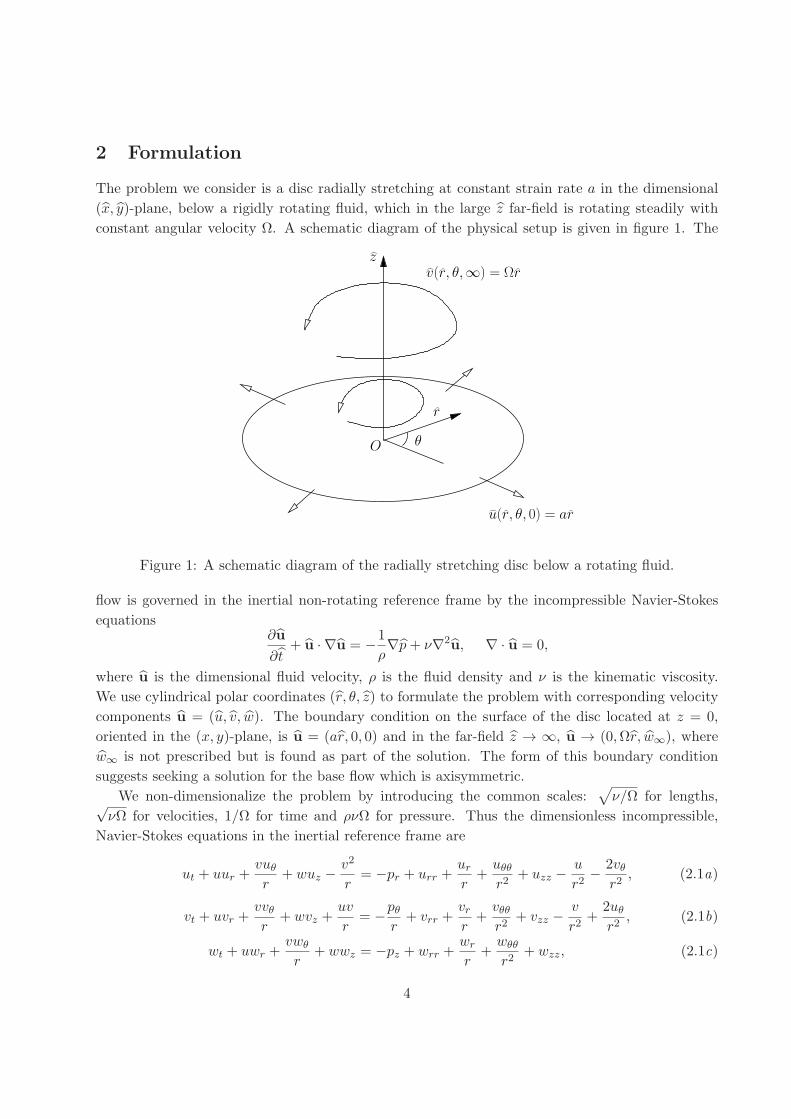
The problem we consider is a disc radially stretching at constant strain rate a in the dimensional

(x, y)-plane, below a rigidly rotating fluid, which in the large z far-field is rotating steadily with

constant angular velocity Ω. A schematic diagram of the physical setup is given in figure 1. The

u(r, θ, 0) = ar

v(r, θ,∞) = Ωr

θ

r

z

O

Figure 1: A schematic diagram of the radially stretching disc below a rotating fluid.

flow is governed in the inertial non-rotating reference frame by the incompressible Navier-Stokes

equations∂u

∂t+ u · ∇u = −1

ρ∇p+ ν∇2

u, ∇ · u = 0,

where u is the dimensional fluid velocity, ρ is the fluid density and ν is the kinematic viscosity.

We use cylindrical polar coordinates (r, θ, z) to formulate the problem with corresponding velocity

components u = (u, v, w). The boundary condition on the surface of the disc located at z = 0,

oriented in the (x, y)-plane, is u = (ar, 0, 0) and in the far-field z → ∞, u → (0,Ωr, w∞), where

w∞ is not prescribed but is found as part of the solution. The form of this boundary condition

suggests seeking a solution for the base flow which is axisymmetric.

We non-dimensionalize the problem by introducing the common scales:√

ν/Ω for lengths,√νΩ for velocities, 1/Ω for time and ρνΩ for pressure. Thus the dimensionless incompressible,

Navier-Stokes equations in the inertial reference frame are

ut + uur +vuθr

+ wuz −v2

r= −pr + urr +

urr

+uθθr2

+ uzz −u

r2− 2vθ

r2, (2.1a)

vt + uvr +vvθr

+ wvz +uv

r= −pθ

r+ vrr +

vrr

+vθθr2

+ vzz −v

r2+

2uθr2

, (2.1b)

wt + uwr +vwθ

r+ wwz = −pz + wrr +

wr

r+

wθθ

r2+ wzz, (2.1c)

4

ur +u

r+

vθr

+ wz = 0, (2.1d)

where (u, v, w) are the dimensionless velocity components, p the dimensionless pressure and (r, θ, z)

are the dimensionless cylindrical polar coordinates. The subscripts in (2.1) denote partial deriva-

tives. In these non-dimensional variables the disc boundary conditions are

u(r, θ, 0) = σr, v(r, θ, 0) = 0, w(r, θ, 0) = 0, (2.2a)

and the far field conditions are

u(r, θ,∞) = 0, v(r, θ,∞) = r, w(r, θ,∞) = w∞, (2.2b)

where w∞ is to be determined. The parameter σ = a/Ω defines a one parameter family of possible

solutions.

2.1 The base flow

The flow can be separated into an axisymmetric steady base flow, and a more general unsteady

part whose amplitude is characterized by a small parameter δ ≪ 1. Thus inserting

u = rf ′(z) + δu(r, θ, z, t), (2.3a)

v = rg(z) + δv(r, θ, z, t), (2.3b)

w = −2f(z) + δw(r, θ, z, t), (2.3c)

p = P (r, z) + δp(r, θ, z, t), (2.3d)

into (2.1) and (2.2) and equating terms at O(1) leads to the coupled pair of nonlinear ordinary

differential equations

f ′′′ + 2ff ′′ − f ′2 + g2 − 1 = 0, (2.4a)

g′′ + 2(fg′ − f ′g) = 0, (2.4b)

to be solved together with the boundary conditions

f(0) = 0, f ′(0) = σ, f ′(∞) = 0 (2.5a)

g(0) = 0, g(∞) = 1. (2.5b)

In (2.3c) the form of the base flow f(z), g(z) is found by the need to satisfy (2.1d) and the primes

in (2.4) denote ordinary derivatives with respect to z. In deriving the above system of ordinary

differential equations it is also possible to compute the base pressure field

p(r, z) = p0 + 2σ2 +1

2r2 − 2(f ′ + f2), (2.6)

where p0 is the constant pressure at (r, z) = (0, 0). The governing ordinary differential equations

(2.4) and the pressure field (2.6) can be shown to agree with (3.11)-(3.16) of Lingwood (1997) when

the Rossby number Ro ≡ 1. Note from (2.3c) that w∞ = −2f(∞).

The radial and azimuthal dimensional shear stresses on the disc surface are given by

τr = ρνΩrf ′′(0), τθ = ρνΩrg′(0).

Numerical results for the base flow equations are investigated in §3.

5

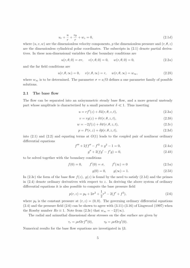
2.2 Linearized disturbance equations

Substituting (2.3) into (2.1) and equating terms of O(δ) furnishes the linearized disturbance equa-

tions

Du+ rf ′′w + f ′u− 2gv = −pr + Lu− u

r2− 2vθ

r2, (2.7a)

Dv + rg′w + f ′v + 2gu = −pθr

+ Lv − v

r2+

2uθr2

, (2.7b)

Dw − 2f ′w = −pz + Lw, (2.7c)

ur +u

r+

vθr

+ wz = 0, (2.7d)

where

D ≡ ∂

∂t− rf ′′

∂

∂r+ g

∂

∂θ− 2f

∂

∂z,and L ≡ 1

r

∂

∂r

(r∂

∂r

)+

1

r2∂2

∂θ2+

∂2

∂z2.

These linear partial differential equations have coefficients which depend upon r and z but not on

θ or t, and therefore we can take Fourier and Laplace transforms respectively. However, since the

resulting disturbance equations remain as partial differential equations in r and z, they can only

be reduced to ordinary differential equations at leading order by considering a point on the disc

far from the flow axis of rotation where the boundary layer profile is assumed to be approximately

parallel. For the stability analysis presented in this paper we shall work in this limiting regime.

If we let R be the dimensional radial position at which we perform a stability analysis of the

flow on the disc, then we can introduce the Reynolds number Re such that

Re = R

√Ω

ν.

We next introduce a new scaled radial coordinate r given by

r = r Re,

where we assume Re ≫ 1, to be far from the flow axis of rotation, and r = O(1) in this region. In

this region we neglect the weak non-parallel effects of the boundary layer on the disc and hypothesize

that the disturbance quantities assume the waveform given by

u(r, θ, z, t) = u(z) exp[iRe

(αr + βθ − ωt

)], (2.8a)

v(r, θ, z, t) = v(z) exp[iRe

(αr + βθ − ωt

)], (2.8b)

w(r, θ, z, t) = w(z) exp[iRe

(αr + βθ − ωt

)], (2.8c)

p(r, θ, z, t) = Rep(z) exp[iRe

(αr + βθ − ωt

)]. (2.8d)

Here α and β are O(1) scaled radial and azimuthal wavenumbers respectively, ω is the scaled angular

frequency, and we have recycled the notation (u, v, w, p) with the understanding that henceforth

these refer only to the perturbation quantities. The presence of the Reynolds number in the

6

exponential terms indicate that the resulting waves are short compared to the distance to the axis

of rotation for the flow field. Thus this is the basis for the WKB approximation in (2.8).

Substituting (2.8) into the linearized disturbance equations (2.7), and taking the limit as

Re → ∞ leads to four ordinary differential equations for (u, v, w, p) which, on eliminating (u, v, p),

reduce to the Rayleigh equation

(Q− ω)(w′′ − γ2w

)−Q′′w = 0, (2.9a)

where

Q(z) = αf ′(z) + βg(z), γ2 = α2 + β2, (2.9b)

β = β/r and the primes denote derivatives with respect to z. Note that Reβ is an integer, but as

we are working in the large Re limit we can consider β to be a real variable. While the disturbance

equation does not depend explicitly on r through the Reynolds number, there is still a radial

dependence on the solutions through the quantity β. The wavenumber α and/or the frequency ω,

are allowed to become complex in order to satisfy the homogenous boundary conditions

w(0) = 0, w(∞) = 0. (2.10)

Hence we perform both a temporal and spatio-temporal stability analysis of (2.9) in §4, calculatingα and ω such that (2.10) is satisfied.

3 Numerical solutions for the base flow

In this section we present numerical results for the solution to the one-parameter system given

by (2.4) and (2.5). The system is solved using a 4th order Runge-Kutta shooting method with

Newton iterations at z = zmax to update the values of f ′′(0) and g′(0) such that the far field

boundary conditions are satisfied; see Press, et al. (1989). The integration domain z ∈ [0, zmax]

and the integration step size are varied to ensure that the results presented here are independent

of these parameters. We find zmax = 20 is large enough to correctly capture the far field boundary

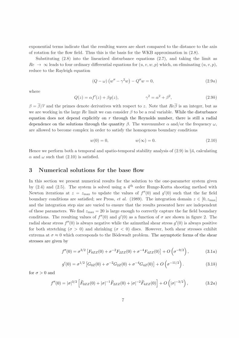
conditions. The resulting values of f ′′(0) and g′(0) as a function of σ are shown in figure 2. The

radial shear stress f ′′(0) is always negative while the azimuthal shear stress g′(0) is always positive

for both stretching (σ > 0) and shrinking (σ < 0) discs. However, both shear stresses exhibit

extrema at σ ≈ 0 which corresponds to the Bodewadt problem. The asymptotic forms of the shear

stresses are given by

f ′′(0) = σ3/2[F0ZZ(0) + σ−2F2ZZ(0) + σ−4F4ZZ(0)

]+O

(σ−9/2

), (3.1a)

g′(0) = σ1/2[G0Z(0) + σ−2G2Z(0) + σ−4G4Z(0)

]+O

(σ−11/2

). (3.1b)

for σ > 0 and

f ′′(0) = |σ|3/2[F0ZZ(0) + |σ|−1F2ZZ(0) + |σ|−2F4ZZ(0)

]+O

(|σ|−3/2

), (3.2a)

7

(a)-30

-25

-20

-15

-10

-5

0

-10 -5 0 5 10

f ′′(0)

σ (b) 0

5

10

15

20

25

30

-10 -5 0 5 10

g′(0)

σ

Figure 2: Plot of the numerical shear stresses (a) f ′′(0) and (b) g′(0) as a function of σ given by thesolid lines and the three-term asymptotic expansions, (3.1) and (3.2), given by the dashed lines.

(a)

0

2

4

6

8

10

-6 -4 -2 0 2 4

z

f ′(z) (b)

0

2

4

6

8

10

0 1 2 3 4 5 6 7 8 9

z

g(z)

σ = −4

σ = 0

σ = −2

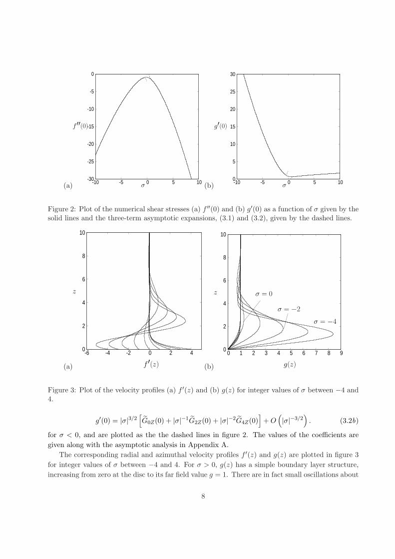
Figure 3: Plot of the velocity profiles (a) f ′(z) and (b) g(z) for integer values of σ between −4 and4.

g′(0) = |σ|3/2[G0Z(0) + |σ|−1G2Z(0) + |σ|−2G4Z(0)

]+O

(|σ|−3/2

). (3.2b)

for σ < 0, and are plotted as the the dashed lines in figure 2. The values of the coefficients are

given along with the asymptotic analysis in Appendix A.

The corresponding radial and azimuthal velocity profiles f ′(z) and g(z) are plotted in figure 3

for integer values of σ between −4 and 4. For σ > 0, g(z) has a simple boundary layer structure,

increasing from zero at the disc to its far field value g = 1. There are in fact small oscillations about

8

g = 1 as z → ∞, but these are not visible in the figure; see §3.1. The radial velocity f ′(z) behaves

similarly, decreasing in magnitude from its value at the disc, σ, to f ′ = 0 as z → ∞. These profiles

are similar to those presented in Sahoo et al. (2014) who studied the Bodewadt problem with an

imposed Navier slip condition at the wall, where the velocity at the wall is given as a multiple of

the shear value at the wall, and thus is found as part of the solution procedure.

For σ ≤ 0, on the other hand, g(z) exhibits a strong wall jet structure in the boundary layer,

the magnitude of which increases as σ decreases, while f ′(z) now includes a region of reverse flow

at the disc. In both cases the oscillations as z → ∞ are now obvious. In order to accurately capture

these oscillations at infinity, it is necessary to compute results to a high degree of precision. For

−5 . σ . 1 we find quadruple precision is required to accurately integrate out to z = 20. Outside

this region double precision is sufficient to produce the required accuracy. Due to the reverse flow

at the surface of the disc, we expect the results for σ ≤ 0 to be more unstable (both convectively

and absolutely) than those for σ > 0. However, the actual stability properties depend on the form

of the ‘effective’ two-dimensional profile Q(z) in (2.2), thus determining the stability properties is

difficult without first knowing the form of Q(z). Before performing the stability analysis, we first

highlight the large z behaviour of the base flow, which highlights the difficulty in solving the base

flow, but also allows for an alternative means for calculating the base flow, integrating from z = ∞to the disc.

3.1 Oscillatory behaviour at large z

It is possible to determine the asymptotic behaviour of the velocity profile at large z by writing

g(z) = 1 + δg(z), f(z) = f∞ + δf(z), (3.3)

where δ is a small parameter and f∞ = f(∞). Substituting these expressions into (2.4) and

retaining only terms at O(δ) leads to the pair of equations

f ′′′ + 2f∞f ′′ + 2g = 0, (3.4a)

g′′ + 2f∞g ′ − 2f ′ = 0. (3.4b)

Substituting (3.4b) into (3.4a) and simplifying leads to the 4th order ordinary differential equation

for g(z)

g(iv) + 4f∞g′′′ + 4f2∞g′′ + 4g = 0. (3.5)

Solving this equation, and retaining only those terms which tend to zero as z → ∞, gives

g(z) = eλrz (A cosλiz +B sinλiz) , (3.6a)

where A and B are constants which are, in principle, determined by the boundary conditions at

the disc and

λr = −f∞ − 1

2

√2f2

∞+ 2

√f4∞

+ 4, λi =2√

2f2∞

+ 2√

f4∞

+ 4. (3.6b)

9

-1

-0.5

0

0.5

1

1.5

2

2.5

-10 -5 0 5 10

f∞

σ

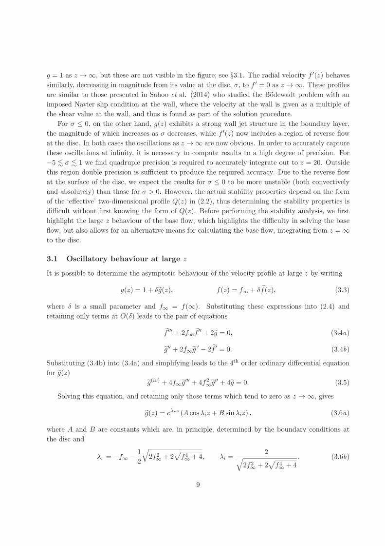
Figure 4: Plot of the constant f∞ = f(∞) from the numerical solution as a function of σ. Thedashed lines represent the large |σ| asymptotic results from Appendix A.

It is clear from the form of λr < 0 and λi > 0 that the constant f∞ is important in determining

the large z behaviour, and is plotted in figure 4.

The exponential form of the solution in (3.6a) and the quadratic nonlinearities which appear

in (2.4) suggest that the large z form can be approximated by expanding in powers of exp(λrz),

essentially δ = 1 in (3.3), and exp(λrz) becomes the small component of the expansion. The first

few terms in the expansion for g(z) are

g(z) ∼ 1 + eλrz (A cosλiz +B sinλiz) + e2λrz (α+ β cosλiz + γ sinλiz) , (3.7)

where the forms of α, β and γ are given in Appendix B. The corresponding form of f(z) can be

found using (3.2b), but as it is not required for the subsequent analysis, we do not express its full

form here.

The undetermined constants A and B in (3.7) are found from the numerical solution by matching

the position of the stationary points, zm of g, and the value of the function, gm = g(zm), at these

points. This furnishes a pair of equations at each stationary point which can be solved to give

A =gme−λrzm

λi(λi cosλizm + λr sinλizm) , B =

gme−λrzm

λi(λi sinλizm − λr cosλizm) . (3.8)

Performing this calculation at each stationary point we find that the values of A and B converge

as the value of zm increases, at least to 4 or 5 significant figures, which we find to be sufficient for

graphical accuracy. The large z form of g(z) (3.7) is plotted together with the numerical solution

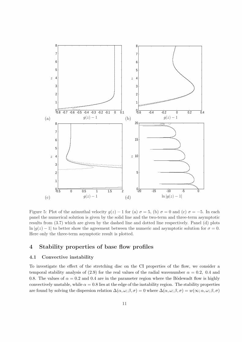
for σ = 5, 0,−5 in figure 5. The values of A and B for these results are given in table 1. We

have found in our study that correctly determining these far field oscillations is important when

undertaking the stability analysis, in the subsequent section.

10

(a)

0

1

2

3

4

5

6

7

8

-0.8 -0.7 -0.6 -0.5 -0.4 -0.3 -0.2 -0.1 0 0.1

z

g(z)− 1 (b)

0

1

2

3

4

5

6

7

8

-0.6 -0.4 -0.2 0 0.2 0.4

z

g(z)− 1

(c)

0

1

2

3

4

5

6

7

8

-0.5 0 0.5 1 1.5 2

z

g(z)− 1 (d)

0

5

10

15

20

-20 -15 -10 -5 0

z

ln |g(z)− 1|

Figure 5: Plot of the azimuthal velocity g(z)− 1 for (a) σ = 5, (b) σ = 0 and (c) σ = −5. In eachpanel the numerical solution is given by the solid line and the two-term and three-term asymptoticresults from (3.7) which are given by the dashed line and dotted line respectively. Panel (d) plotsln |g(z)− 1| to better show the agreement between the numeric and asymptotic solution for σ = 0.Here only the three-term asymptotic result is plotted.

4 Stability properties of base flow profiles

4.1 Convective instability

To investigate the effect of the stretching disc on the CI properties of the flow, we consider a

temporal stability analysis of (2.9) for the real values of the radial wavenumber α = 0.2, 0.4 and

0.8. The values of α = 0.2 and 0.4 are in the parameter region where the Bodewadt flow is highly

convectively unstable, while α = 0.8 lies at the edge of the instability region. The stability properties

are found by solving the dispersion relation ∆(α, ω;β, σ) = 0 where ∆(α, ω;β, σ) = w(∞;α, ω;β, σ)

11

σ A B

-5 346.0600 1377.758960 -1.04752 0.237775 -0.41458 -6.28651

Table 1: Table of values of A and B from (3.6) used in figure 5.

is found by solving (2.9) for a given base velocity profileQ(z) ensuring the boundary condition (2.10)

at z = ∞ is satisfied. This quantity equals zero when the correct value of ω is chosen for a given α.

The dispersion relation is solved using the same shooting process as used for the base flow. In this

section we investigate how the range of azimuthal wavenumbers, β, over which the flow is unstable

(Im(ω) = ωi > 0) varies with σ. In a CI analysis we are interested in the growth of individual

waves not their interaction with each other.

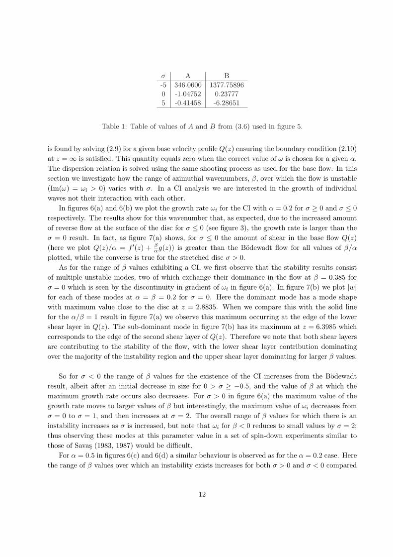
In figures 6(a) and 6(b) we plot the growth rate ωi for the CI with α = 0.2 for σ ≥ 0 and σ ≤ 0

respectively. The results show for this wavenumber that, as expected, due to the increased amount

of reverse flow at the surface of the disc for σ ≤ 0 (see figure 3), the growth rate is larger than the

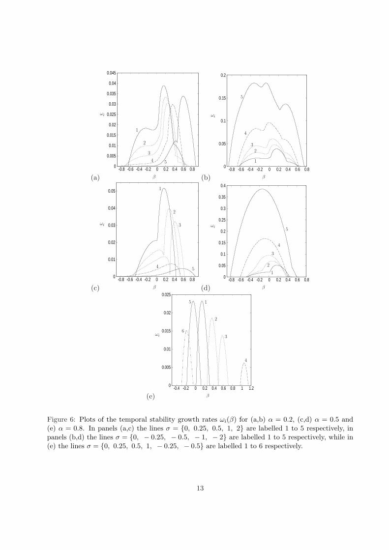
σ = 0 result. In fact, as figure 7(a) shows, for σ ≤ 0 the amount of shear in the base flow Q(z)

(here we plot Q(z)/α = f ′(z) + βαg(z)) is greater than the Bodewadt flow for all values of β/α

plotted, while the converse is true for the stretched disc σ > 0.

As for the range of β values exhibiting a CI, we first observe that the stability results consist

of multiple unstable modes, two of which exchange their dominance in the flow at β = 0.385 for

σ = 0 which is seen by the discontinuity in gradient of ωi in figure 6(a). In figure 7(b) we plot |w|for each of these modes at α = β = 0.2 for σ = 0. Here the dominant mode has a mode shape

with maximum value close to the disc at z = 2.8835. When we compare this with the solid line

for the α/β = 1 result in figure 7(a) we observe this maximum occurring at the edge of the lower

shear layer in Q(z). The sub-dominant mode in figure 7(b) has its maximum at z = 6.3985 which

corresponds to the edge of the second shear layer of Q(z). Therefore we note that both shear layers

are contributing to the stability of the flow, with the lower shear layer contribution dominating

over the majority of the instability region and the upper shear layer dominating for larger β values.

So for σ < 0 the range of β values for the existence of the CI increases from the Bodewadt

result, albeit after an initial decrease in size for 0 > σ ≥ −0.5, and the value of β at which the

maximum growth rate occurs also decreases. For σ > 0 in figure 6(a) the maximum value of the

growth rate moves to larger values of β but interestingly, the maximum value of ωi decreases from

σ = 0 to σ = 1, and then increases at σ = 2. The overall range of β values for which there is an

instability increases as σ is increased, but note that ωi for β < 0 reduces to small values by σ = 2;

thus observing these modes at this parameter value in a set of spin-down experiments similar to

those of Savas (1983, 1987) would be difficult.

For α = 0.5 in figures 6(c) and 6(d) a similar behaviour is observed as for the α = 0.2 case. Here

the range of β values over which an instability exists increases for both σ > 0 and σ < 0 compared

12

(a)

0

0.005

0.01

0.015

0.02

0.025

0.03

0.035

0.04

0.045

-0.8 -0.6 -0.4 -0.2 0 0.2 0.4 0.6 0.8

β

ωi

1

3

4 5

2

(b)

0

0.05

0.1

0.15

0.2

-0.8 -0.6 -0.4 -0.2 0 0.2 0.4 0.6 0.8

β

ωi

1

3

4

5

2

(c)

0

0.01

0.02

0.03

0.04

0.05

-0.8 -0.6 -0.4 -0.2 0 0.2 0.4 0.6 0.8

β

ωi

1

3

45

2

(d)

0

0.05

0.1

0.15

0.2

0.25

0.3

0.35

0.4

-0.8 -0.6 -0.4 -0.2 0 0.2 0.4 0.6 0.8

β

ωi

1

3

4

5

2

(e)

0

0.005

0.01

0.015

0.02

0.025

-0.4 -0.2 0 0.2 0.4 0.6 0.8 1 1.2

β

ωi

1

3

4

5

2

6

Figure 6: Plots of the temporal stability growth rates ωi(β) for (a,b) α = 0.2, (c,d) α = 0.5 and(e) α = 0.8. In panels (a,c) the lines σ = 0, 0.25, 0.5, 1, 2 are labelled 1 to 5 respectively, inpanels (b,d) the lines σ = 0, − 0.25, − 0.5, − 1, − 2 are labelled 1 to 5 respectively, while in(e) the lines σ = 0, 0.25, 0.5, 1, − 0.25, − 0.5 are labelled 1 to 6 respectively.

13

(a) 0

2

4

6

8

10

0 1 2 3 4 5 6

z

βα = 1

βα = −1

2βα = 1

2

(b)

0

2

4

6

8

10

12

14

0 0.2 0.4 0.6 0.8 1 1.2

z

|w|

1

2

Figure 7: (a) Plot of f ′(z) + βαg(z), for

βα = 1, 1/2,−1/2 The three cases are separated by a

constant, and in each case the solid line represents σ = 0, the long dashed line represents σ = 0.5and the short dashed line represents σ = −0.5. (b) Plot of |w|, for α = β = 0.2 and σ = 0. Result 1represents the dominant eigenmode with ω = 0.0725+0.0278i while result 2 gives the sub-dominanteigenmode mode with ω = 0.2312 + 0.0094i.

to the Bodewadt result. The significant difference at this wavenumber is the rate at which the

maximum value of ωi increases for σ < 0 and decreases for σ > 0 is much larger than for α = 0.2.

Also note that here the maximum value of ωi continues to decrease at σ = 2, unlike in the α = 0.2

case, thus showing that the form of Q(z) for σ = 2 is more unstable to long waves (small α) but

more stable to shorter waves (larger α).

For α = 0.8 in figure 6(e) it is a different story. Here the size of the azimuthal wavenumber

region is approximately constant for the different values of σ considered, but the position of the

instability region varies. Note that here the corresponding results for σ = 2, −1 and −2 are stable.

The results in this section indicate that the region of azimuthal wavenumbers for CI typically

increases for a small to moderate fixed value of α when the disc is both stretched (σ > 0) and

shrunk (σ < 0). The corresponding behaviour for AI is considered in §4.2 with particular interest

on how individual modes interact with one another.

4.2 Absolute instability

While the CI of a flow depends on the stability of individual waves, its AI is a consequence of the

interaction of these waves as they propagate as wavepackets. The calculation of the response of the

base flow to infinitesimal perturbations in a frame of reference fixed on the disturbance position

for both the Bodewadt and Ekman layer flows can be found in Lingwood (1997), and for the von

Karman flow in Lingwood (1995). We apply the same fundamental approach to the base flows in

this paper.

14

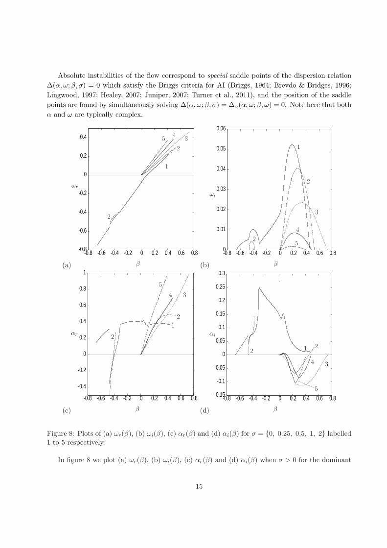
Absolute instabilities of the flow correspond to special saddle points of the dispersion relation

∆(α, ω;β, σ) = 0 which satisfy the Briggs criteria for AI (Briggs, 1964; Brevdo & Bridges, 1996;

Lingwood, 1997; Healey, 2007; Juniper, 2007; Turner et al., 2011), and the position of the saddle

points are found by simultaneously solving ∆(α, ω;β, σ) = ∆α(α, ω;β, ω) = 0. Note here that both

α and ω are typically complex.

(a)

-0.8

-0.6

-0.4

-0.2

0

0.2

0.4

-0.8 -0.6 -0.4 -0.2 0 0.2 0.4 0.6 0.8

β

ωr

1

2

34

5

2

(b)

0

0.01

0.02

0.03

0.04

0.05

0.06

-0.8 -0.6 -0.4 -0.2 0 0.2 0.4 0.6 0.8

β

ωi

1

2

3

4

52

(c)

-0.4

-0.2

0

0.2

0.4

0.6

0.8

1

-0.8 -0.6 -0.4 -0.2 0 0.2 0.4 0.6 0.8

β

αr

1

2

34

5

2

(d)

-0.15

-0.1

-0.05

0

0.05

0.1

0.15

0.2

0.25

0.3

-0.8 -0.6 -0.4 -0.2 0 0.2 0.4 0.6 0.8

β

αi

1 2

34

5

2

Figure 8: Plots of (a) ωr(β), (b) ωi(β), (c) αr(β) and (d) αi(β) for σ = 0, 0.25, 0.5, 1, 2 labelled1 to 5 respectively.

In figure 8 we plot (a) ωr(β), (b) ωi(β), (c) αr(β) and (d) αi(β) when σ > 0 for the dominant

15

saddle point for values of β where the flow is absolutely unstable. Here the stretching parameter

takes the values σ = 0, 0.25, 0.5, 1, 2. The result for σ = 0 is the Bodewadt result presented in

figure 9(b) and 9(d) of Lingwood (1997) (denoted by the Rossby number Ro = 1). We note that

while our results are in good agreement with those of Lingwood (1997) for β > 0, we obtain subtly

different results for β < 0. However our results are qualitatively similar to those of Lingwood

(1997) when her Rossby number is Ro = 0.9 and 0.8 in the range −0.3 ≤ β ≤ 0. We believe this

discrepancy is due to the difficulty in accurately calculating the base flow for this value of σ, as

described in §3. The fact that our results demonstrate qualitative agreement in behaviour with the

Ro = 0.9 and 0.8 results of Lingwood (1997) gives us confidence in our numerical procedure.

The Bodewadt result has a maximum growth rate at β = 0.1871 and the AI extends over the

range of azimuthal wavenumbers β ∈ [−0.6659, 0.4605]. At β = −0.4096 there exists a second,

smaller, maximum growth rate which is caused by a second saddle point on the inversion contour

becoming the dominant saddle point. As the disc stretching rate is increased to σ = 0.25 the

two maximum growth rate values decrease in magnitude, and in fact the AI actually vanishes

for a range of β values between these two maxima. The two maxima move to β = 0.2725 and

β = −0.4364 respectively, and the flow is absolutely unstable for azimuthal wavenumbers β ∈[−0.4673,−0.3785]∪ [0.0001, 0.5280]. As σ increases to 0.5, the flow is no longer absolutely unstable

for β < 0, but the positive range of β for which an AI exists is larger still. Beyond this value, the

range of β values for the AI decreases and for σ = 2 the flow is only absolutely unstable for

β ∈ [0, 0.3991], but this instability is weak, with a maximum growth rate of ωi = 1.773 × 10−3.

Note that this result is in contrast to the CI result in figure 6 which shows the range of β values

for CI increases as σ is increased from σ = 0, and at σ = 2, the magnitude of ωi for the CI is much

larger.

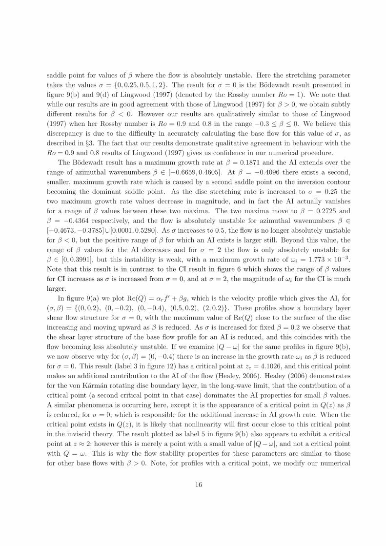
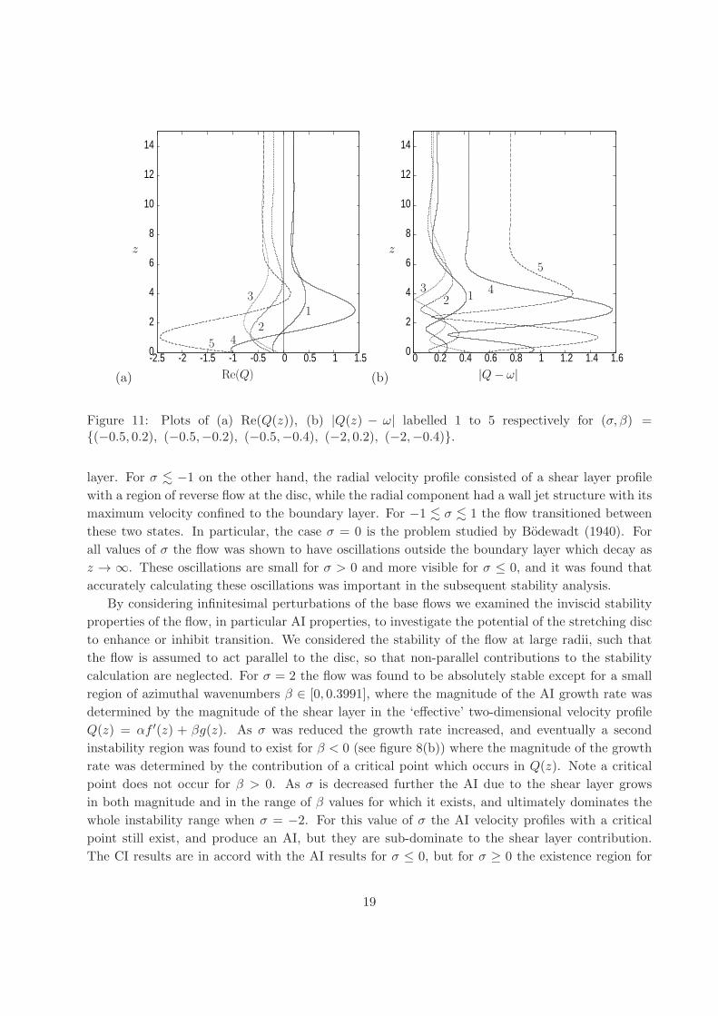
In figure 9(a) we plot Re(Q) = αrf′ + βg, which is the velocity profile which gives the AI, for

(σ, β) = (0, 0.2), (0,−0.2), (0,−0.4), (0.5, 0.2), (2, 0.2). These profiles show a boundary layer

shear flow structure for σ = 0, with the maximum value of Re(Q) close to the surface of the disc

increasing and moving upward as β is reduced. As σ is increased for fixed β = 0.2 we observe that

the shear layer structure of the base flow profile for an AI is reduced, and this coincides with the

flow becoming less absolutely unstable. If we examine |Q− ω| for the same profiles in figure 9(b),

we now observe why for (σ, β) = (0,−0.4) there is an increase in the growth rate ωi as β is reduced

for σ = 0. This result (label 3 in figure 12) has a critical point at zc = 4.1026, and this critical point

makes an additional contribution to the AI of the flow (Healey, 2006). Healey (2006) demonstrates

for the von Karman rotating disc boundary layer, in the long-wave limit, that the contribution of a

critical point (a second critical point in that case) dominates the AI properties for small β values.

A similar phenomena is occurring here, except it is the appearance of a critical point in Q(z) as β

is reduced, for σ = 0, which is responsible for the additional increase in AI growth rate. When the

critical point exists in Q(z), it is likely that nonlinearity will first occur close to this critical point

in the inviscid theory. The result plotted as label 5 in figure 9(b) also appears to exhibit a critical

point at z ≈ 2; however this is merely a point with a small value of |Q−ω|, and not a critical point

with Q = ω. This is why the flow stability properties for these parameters are similar to those

for other base flows with β > 0. Note, for profiles with a critical point, we modify our numerical

16

(a)

0

2

4

6

8

10

12

14

-0.6 -0.4 -0.2 0 0.2 0.4 0.6 0.8 1Re(Q)

z

12

3

4 5

(b)

0

2

4

6

8

10

12

14

0 0.05 0.1 0.15 0.2 0.25|Q− ω|

z

1

2

3

4

5

Figure 9: Plot of (a) Re(Q(z)), (b) |Q(z) − ω| labelled 1 to 5 respectively for (σ, β) =(0, 0.2), (0,−0.2), (0,−0.4), (0.5, 0.2), (2, 0.2).

scheme to integrate up to the critical layer and then jump to the other side without modifying w

or dw/dz. We can do this because we consider the critical layer to be nonlinear and not viscous

(Benney & Bergeron, 1969).

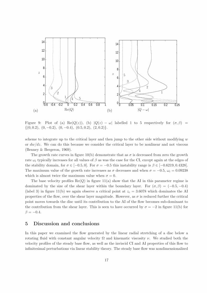
The growth rate curves in figure 10(b) demonstrate that as σ is decreased from zero the growth

rate ωi typically increases for all values of β as was the case for the CI, except again at the edges of

the stability domain, for σ ∈ [−0.5, 0]. For σ = −0.5 this instability range is β ∈ [−0.6219, 0.4328].

The maximum value of the growth rate increases as σ decreases and when σ = −0.5, ωi = 0.09238

which is almost twice the maximum value when σ = 0.

The base velocity profiles Re(Q) in figure 11(a) show that the AI in this parameter regime is

dominated by the size of the shear layer within the boundary layer. For (σ, β) = (−0.5,−0.4)

(label 3) in figure 11(b) we again observe a critical point at zc = 3.6078 which dominates the AI

properties of the flow, over the shear layer magnitude. However, as σ is reduced further the critical

point moves towards the disc until its contribution to the AI of the flow becomes sub-dominant to

the contribution from the shear layer. This is seen to have occurred by σ = −2 in figure 11(b) for

β = −0.4.

5 Discussion and conclusions

In this paper we examined the flow generated by the linear radial stretching of a disc below a

rotating fluid with constant angular velocity Ω and kinematic viscosity ν. We studied both the

velocity profiles of the steady base flow, as well as the inviscid CI and AI properties of this flow to

infinitesimal perturbations via linear stability theory. The steady base flow was nondimensionalised

17

(a)

-2

-1.5

-1

-0.5

0

0.5

1

-1 -0.8 -0.6 -0.4 -0.2 0 0.2 0.4 0.6

β

ωr1

3

4

5

2

(b)

0

0.05

0.1

0.15

0.2

0.25

0.3

0.35

0.4

-1 -0.8 -0.6 -0.4 -0.2 0 0.2 0.4 0.6

β

ωi

1

3

4

5

2

(c)

-0.4

-0.2

0

0.2

0.4

0.6

-1 -0.8 -0.6 -0.4 -0.2 0 0.2 0.4 0.6

β

αr

1

2

3

4

5

2

1

4

(d)

-0.05

0

0.05

0.1

0.15

0.2

0.25

0.3

-1 -0.8 -0.6 -0.4 -0.2 0 0.2 0.4 0.6

β

αi

1

2

3

45

4

2

Figure 10: Plots of (a) ωr(β), (b) ωi(β), (c) αr(β) and (d) αi(β) labelled 1 to 5 respectively forσ = 0, − 0.25, − 0.5, − 1, − 2.

and solely characterised by a single nondimensional parameter σ = a/Ω, where a is the radial rate

of strain of the disc. Numerical results of the base flow equations showed that the radial component

of the shear stress on the disc is always directed towards the origin, while the azimuthal component

of the disc shear stress is directed in the positive θ-direction.

For σ & 1 the radial velocity component consisted of a velocity profile which obtained its

maximum value at the surface of the disc and decreased to zero outside the boundary layer, while

the azimuthal component was zero at the disc and increased to a unit value outside the boundary

18

(a)

0

2

4

6

8

10

12

14

-2.5 -2 -1.5 -1 -0.5 0 0.5 1 1.5Re(Q)

z

1

2

3

45

(b)

0

2

4

6

8

10

12

14

0 0.2 0.4 0.6 0.8 1 1.2 1.4 1.6|Q− ω|

z

123 4

5

Figure 11: Plots of (a) Re(Q(z)), (b) |Q(z) − ω| labelled 1 to 5 respectively for (σ, β) =(−0.5, 0.2), (−0.5,−0.2), (−0.5,−0.4), (−2, 0.2), (−2,−0.4).

layer. For σ . −1 on the other hand, the radial velocity profile consisted of a shear layer profile

with a region of reverse flow at the disc, while the radial component had a wall jet structure with its

maximum velocity confined to the boundary layer. For −1 . σ . 1 the flow transitioned between

these two states. In particular, the case σ = 0 is the problem studied by Bodewadt (1940). For

all values of σ the flow was shown to have oscillations outside the boundary layer which decay as

z → ∞. These oscillations are small for σ > 0 and more visible for σ ≤ 0, and it was found that

accurately calculating these oscillations was important in the subsequent stability analysis.

By considering infinitesimal perturbations of the base flows we examined the inviscid stability

properties of the flow, in particular AI properties, to investigate the potential of the stretching disc

to enhance or inhibit transition. We considered the stability of the flow at large radii, such that

the flow is assumed to act parallel to the disc, so that non-parallel contributions to the stability

calculation are neglected. For σ = 2 the flow was found to be absolutely stable except for a small

region of azimuthal wavenumbers β ∈ [0, 0.3991], where the magnitude of the AI growth rate was

determined by the magnitude of the shear layer in the ‘effective’ two-dimensional velocity profile

Q(z) = αf ′(z) + βg(z). As σ was reduced the growth rate increased, and eventually a second

instability region was found to exist for β < 0 (see figure 8(b)) where the magnitude of the growth

rate was determined by the contribution of a critical point which occurs in Q(z). Note a critical

point does not occur for β > 0. As σ is decreased further the AI due to the shear layer grows

in both magnitude and in the range of β values for which it exists, and ultimately dominates the

whole instability range when σ = −2. For this value of σ the AI velocity profiles with a critical

point still exist, and produce an AI, but they are sub-dominate to the shear layer contribution.

The CI results are in accord with the AI results for σ ≤ 0, but for σ ≥ 0 the existence region for

19

the CI increases with increasing σ, at least up to σ = 2 considered here.

Acknowledgement

The authors would like to thank the anonymous referees whose comments have led to an im-

proved version of this paper.

A Asymptotic analysis for |σ| ≫ 1

In this appendix we consider the asymptotic form of the base flow for large disc stretching and

shrinking rates |σ|. We consider the two asymptotic regimes of a rapid stretching disc σ ≫ 1 and

a rapidly shrinking disc −σ ≫ 1.

A.1 The rapidly stretching disc: σ ≫ 1

The velocity profiles in figure 3 for σ > 0 suggests for large positive σ there exists a boundary

layer close to the disc. The thickness of this boundary layer is O(σ1/2), outside this layer the outer

solution is trivially

g(z) = 1, f(z) = f∞. (A.1)

The inner solution is found by introducing a new stretched boundary layer variable Z, such

that z = |σ|1/2Z, and the scaled inner functions F (Z) and G(Z)

f = σ1/2F (Z), g = G(Z). (A.2)

Introducing these scaled variables into (2.4) leads to

FZZZ + 2FFZZ − F 2Z + σ−2

(G2 − 1

)= 0, F (0) = 0, FZ(0) = 1, FZ(∞) = 0, (A.3a)

GZZ + 2(FGZ − FZG) = 0, G(0) = 0, G(∞) = 1. (A.3b)

We seek an asymptotic solution to these equations where we expand F (Z) and G(Z) in powers

of σ−2

F (Z) = F0(Z) + σ−2F2(Z) + σ−4F4(Z) +O(σ−6

),

G(Z) = G0(Z) + σ−2G2(Z) + σ−4G4(Z) +O(σ−6

).

Inserting these expansions into (3.8) and equating powers of σ−2 leads to the following hierarchy

of system equations: at O(1)

F0ZZZ + 2F0F0ZZ − F 20Z = 0, F0(0) = 0, F0Z(0) = 1, F0Z(∞) = 0,

G0ZZ + 2(F0G0Z − F0ZG0) = 0, G0(0) = 0, G0(∞) = 1;

20

then at O(σ−2)

F2ZZZ + 2 (F0F2ZZ + F2F0ZZ)− 2F0ZF2Z +G20 − 1 = 0,

F2(0) = 0, F2Z(0) = 0, F2Z(∞) = 0,

G2ZZ + 2(F0G2Z + F2G0Z − F0ZG2 − F2ZG0) = 0,

G2(0) = 0, G2(∞) = 0;

and at O(σ−4)

F4ZZZ + 2 (F0F4ZZ + F2F2ZZ + F4F0ZZ)− 2F0ZF4Z − F 22Z + 2G0G2 = 0,

F4(0) = 0, F4Z(0) = 0, F4Z(∞) = 0,

G4ZZ + 2(F0G4Z + F2G2Z + F4G0Z − F0ZG4 − F2ZG2 − F4ZG0) = 0,

G4(0) = 0, G4(∞) = 0.

These systems of equations are solved consecutively using the same numerical scheme as for the

full system.

The resulting asymptotic shear stress values are found to be

F0ZZ(0) = −1.173720738913, G0Z(0) = 0.528652929118,

F2ZZ(0) = −0.772897415441, G2Z(0) = 0.203722589589,

F4ZZ(0) = 0.114592927248, G4Z(0) = −0.071141123212.

A.2 The rapidly shrinking disc: −σ ≫ 1

For σ < 0 the boundary layer thickness is again O(|σ|1/2), and the outer solution is also (A.1).

Using the same boundary layer variable Z as in Appendix A.1 but the scaled inner functions F (Z)

and G(Z)

f = |σ|1/2F (Z), g = |σ|G(Z).

in (2.4) leads to the system

FZZZ + 2F FZZ − F 2Z + G2 − |σ|−2 = 0, F (0) = 0, FZ(0) = −1, FZ(∞) = 0, (A.4a)

GZZ + 2(F GZ − FZG) = 0, G(0) = 0, G(∞) = |σ|−1. (A.4b)

The |σ|−1 term in the boundary condition for G suggests an asymptotic solution in the form

F (Z) = F0(Z) + |σ|−1F1(Z) + |σ|−2F2(Z) +O(|σ|−3

),

G(Z) = G0(Z) + |σ|−1G1(Z) + |σ|−2G2(Z) +O(|σ|−3

).

21

Inserting these expansions into (3.10) and equating powers of |σ|−1 leads to the following hierarchy

of system equations: at O(1)

F0ZZZ + 2F0F0ZZ − F 20Z + G2

0 = 0 F0(0) = 0, F0Z(0) = −1, F0Z(∞) = 0,

G0ZZ + 2(F0G0Z − F0ZG0) = 0 G0(0) = 0, G0(∞) = 0;

then at O(|σ|−1)

F1ZZZ + 2(F0F1ZZ + F1F0ZZ

)− 2F0Z F1Z + 2G0G1 = 0

F1(0) = 0, F1Z(0) = 0, F1Z(∞) = 0,

G1ZZ + 2(F0G1Z + F1G0Z − F0ZG1 − F1ZG0

)= 0

G1(0) = 0, G1(∞) = 1;

and at O(|σ|−2)

F2ZZZ + 2(F0F2ZZ + F1F1ZZ + F2F0ZZ

)− 2F0Z F2Z − F 2

1Z + 2G0G2 + G21 − 1 = 0,

F2(0) = 0, F2Z(0) = 0, F2Z(∞) = 0,

G2ZZ + 2(F0G2Z + F1G1Z + F2G0Z − F0ZG2 − F1ZG1 − F2ZG0

)= 0,

G2(0) = 0, G2(∞) = 0.

Numerically solving these systems give the asymptotic shear stress values as

F0ZZ(0) = −0.725131902079, G0Z(0) = 1.157973962096,

F1ZZ(0) = −0.000000000088, G1Z(0) = 0.000000000018,

F2ZZ(0) = −0.633741006320, G2Z(0) = 0.690472088227.

B Coefficients of the large z asymptotic expansion

In the large-z asymptotic form of g(z) in (3.7) the coefficients α, β and γ are given by

α =ζ1 + ζ2

8 (8f∞λ3r + 4λ4

r + 4f2∞λ2r + 1)

,

β =1

8(π21 + π2

2)(π1(ζ1 − ζ2) + π2ζ3) ,

γ =1

8(π21 + π2

2)(−π2(ζ1 − ζ2) + π1ζ3) ,

22

where

π1 = 8f∞λ3r − 24f∞λ2

iλr + 4λ4i − 24λ2

iλ2r + 4λ4

r − 4f2∞λ2i + 4f2

∞λ2r + 1,

π2 = −8λi(f∞ + 2λr)(f∞λr − λ2i + λ2

r),

ζ1 =1

2

(8f2

∞λ2i − 4f2

∞λ2r + 4f∞λ2

iλr − 4f∞λ3r + λ4

i − 4λ2iλ

2r − λ4

r − 4)A2

−λ2i

(4f∞λr − λ2

i + 5λ2r − 2f2

∞

)B2

−2λi (f∞ + λr)(2f∞λr − λ2

i + λ2r

)AB,

ζ2 = −λ2i

(4f∞λr − λ2

i + 5λ2r − 2f2

∞

)A2

+1

2

(8f2

∞λ2i − 4f2

∞λ2r + 4f∞λ2

iλr − 4f∞λ3r + λ4

i − 4λ2iλ

2r − λ4

r − 4)B2

+2λi (f∞ + λr)(2f∞λr − λ2

i + λ2r

)AB,

ζ3 = 2λi (f∞ + λr)(2f∞λr − λ2

i + λ2r

)(A2 −B2)

+(4f2

∞λ2i − 4f2

∞λ2r + 12f∞λ2

iλr − 4f∞λ3r − λ4

i + 6λ2iλ

2r − λ4

r − 4)AB.

References

Bodewadt, U. T. 1940 Die Drehstromung uber festem Grunde. Z. Angew Math. Mech. 20, 241-

253

Benney, D. J. & Bergeron, R. F. 1969 A new class of nonlinear waves in parallel flows. Stud.

Appl. Maths. 48, 181-204

Brevdo, L. & Bridges, T. J. 1996 Absolute and convective instabilities of spatially periodic

flows. Philos. Trans. R. Soc. London Ser. A. 354(1710), 1027-1064

Briggs, R. J. 1964 Electron–Stream Interaction with Plasmas. MIT Press

Ekman, V. W. 1905 On the influence of the Earth’s rotation on ocean currents. Ark. Mat. Astr.

Fys. 2(11)

Fernandez-Feria, R. 2002 Axisymmetric instabilities of Bodewadt flow. Phys. Fluids. 12, 1730-

1739

Healey, J. J. 2006 Long-Wave Theory for the Absolute Instability of the Rotating-Disc Boundary

Layer. Proc. Roy. Soc. 462(2069), 1467-1492

Healey, J. J. 2007 Enhancing the absolute instability of a boundary layer by adding a far-away

plate. J. Fluid Mech. 579, 29-61

Huerre, P. and Monkewitz, P. A. 1990 Local and global instabilities in spatially developing

flows. Ann. Rev. Fluid Mech. 22, 473-537

23

Itoh, M., Yamada, Y., Imao, S. & Gonda, M. 1990 Experiments on turbine flow due to an

enclosed rotating disc. Proceedings of the first symposium on measurments engineering turbulence

modelling (ed. W. Rodi & E. C. Canic), 659-668. Elsevier (New York).

Juniper, M. P. 2007 The full impulse response of two-dimensional jet/wake flows and implications

for confinement. J. Fluid Mech. 590, 163-185

Karman, Th. von 1921 Uber laminare und turbulente Reibung. Z. Angew Math. Mech. 1, 233-252

Lingwood, R. J. 1995 Absolute instability of the boundary layer on a rotating disk. J. Fluid

Mech. 299, 17-33

Lingwood, R. J. 1997 Absolute instability of the Ekman layer and related rotating flows. J. Fluid

Mech. 331, 405-428

Lopez, J. M. & Weidman, P. D. 1996 Stability of stationary endwall boundary layers during

spin-down. J. Fluid Mech. 326, 373-398

Mackerrell, S. O. 2005 Stability of Bodewadt Flow. Philos. Trans. R. Soc. London Ser. A.

363(1830), 1181-1188

Owen, J. M. 1988 Air-cooled gas turbine discs: a review of recent research. TFMRC Report.

University of Sussex

Press, W. H., Flannery, B. P., Teukolsky, S. A. & Vetterling, W. T. 1989 Numerical

recipes (FORTRAN version). Cambridge University Press (Cambridge)

Sahoo, B., Abbasbandy, S. and Poncet, S. 2014 A brief note on the computation of the

Bodewadt flow with Navier slip boundary conditions. Comput. & Fluids. 90, 133-137

Savas, O. 1983 Circular waves on stationary disk in rotating flow. Phys. Fluids. 26, 3445-3448

Savas, O. 1987 Stability of Bodewadt flow. J. Fluid Mech. 183, 77-94

Schmid, P. J. and Henningson, D. S. 2001 Stability and Transition in Shear Flows. Springer

(New York)

Turner, M. R., Healey, J. J., Sazhin, S. S. and Piazzesi, R. 2011 Stability analysis and

break–up length calculations for steady planar liquid jets. J. Fluid Mech. 668, 384-411

24