32-1

Lecture 32

Analysis of Covariance II

STAT 512

Spring 2011

Background Reading

KNNL: Chapter 22

32-2

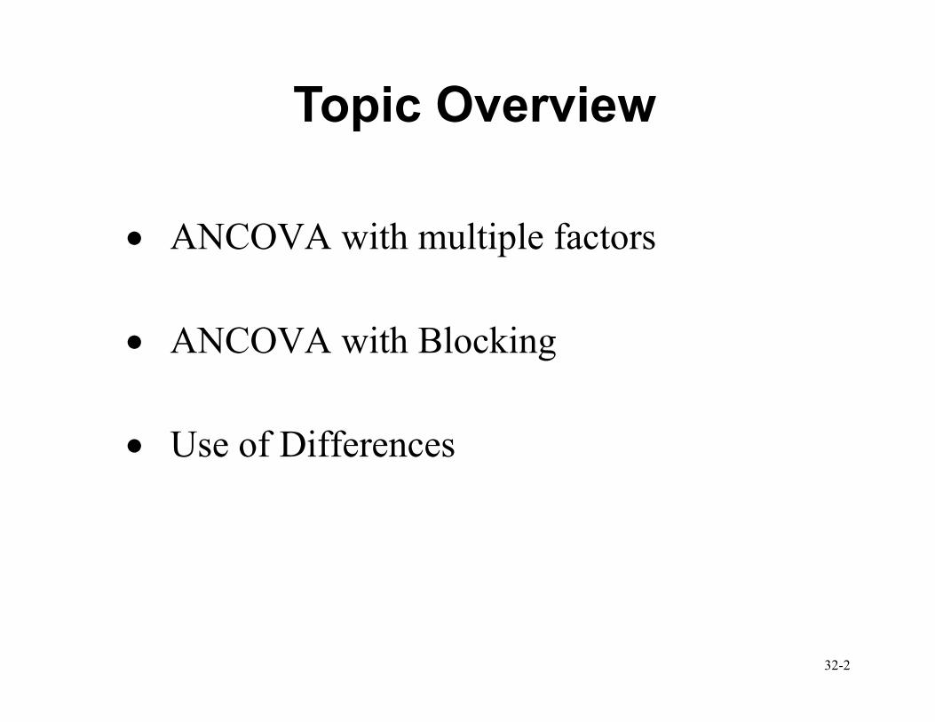
Topic Overview

ANCOVA with multiple factors

ANCOVA with Blocking

Use of Differences

32-3

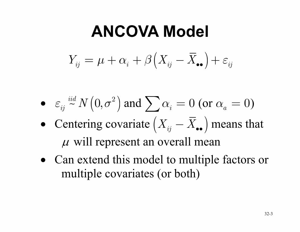
ANCOVA Model

( )ij i ij ijY X X = + + +

( )2~ 0,iidij N and 0i = (or 0a = ) Centering covariate ( )ijX X means that

will represent an overall mean

Can extend this model to multiple factors or

multiple covariates (or both)

32-4

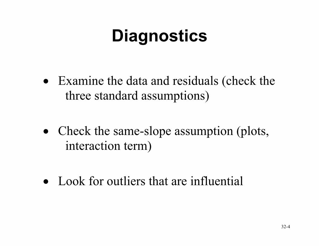
Diagnostics

Examine the data and residuals (check the

three standard assumptions)

Check the same-slope assumption (plots,

interaction term)

Look for outliers that are influential

32-5

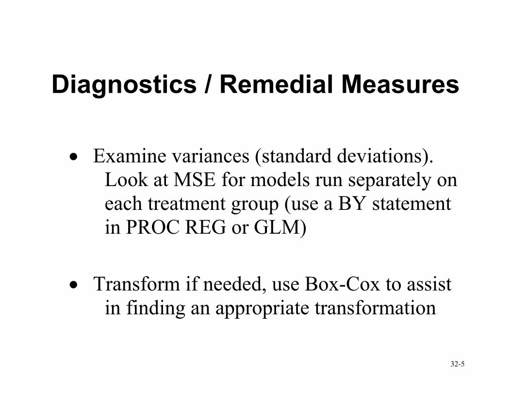
Diagnostics / Remedial Measures

Examine variances (standard deviations).

Look at MSE for models run separately on

each treatment group (use a BY statement

in PROC REG or GLM)

Transform if needed, use Box-Cox to assist

in finding an appropriate transformation

32-6

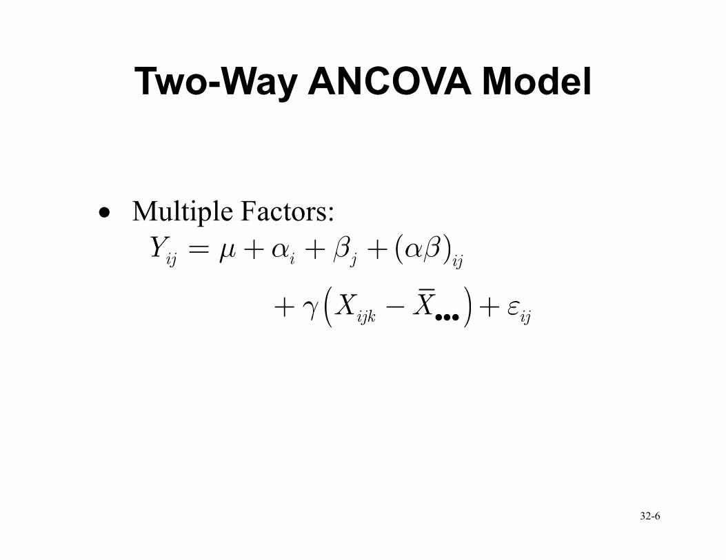
Two-Way ANCOVA Model

Multiple Factors:

( )

( ) ij i j ij

ijk ij

Y

X X

= + + +

+ +

32-7

Two-Way ANCOVA Model (2)

Basic idea remains the same. For each

treatment combination we have a linear

regression in which the slopes are the

same, but the intercepts may differ.

We make comparisons using least-square

means, with the covariates set to their

mean values (so that any differences will

not be due to the level of the covariates)

32-8

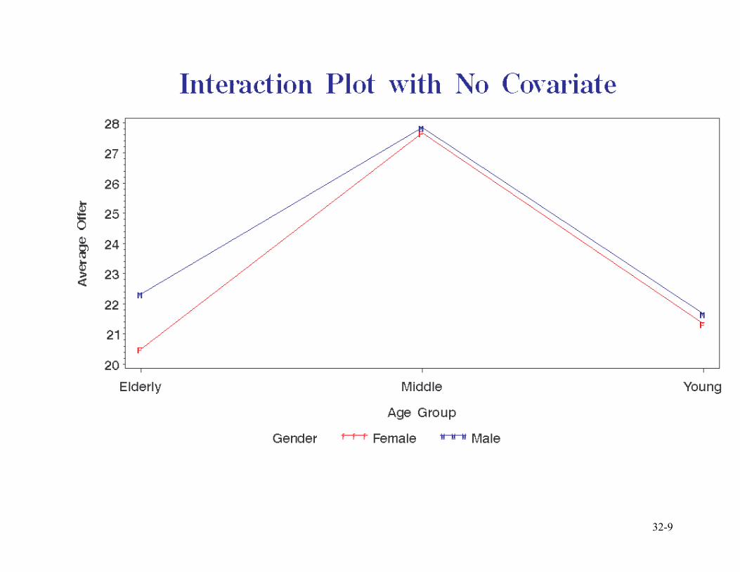
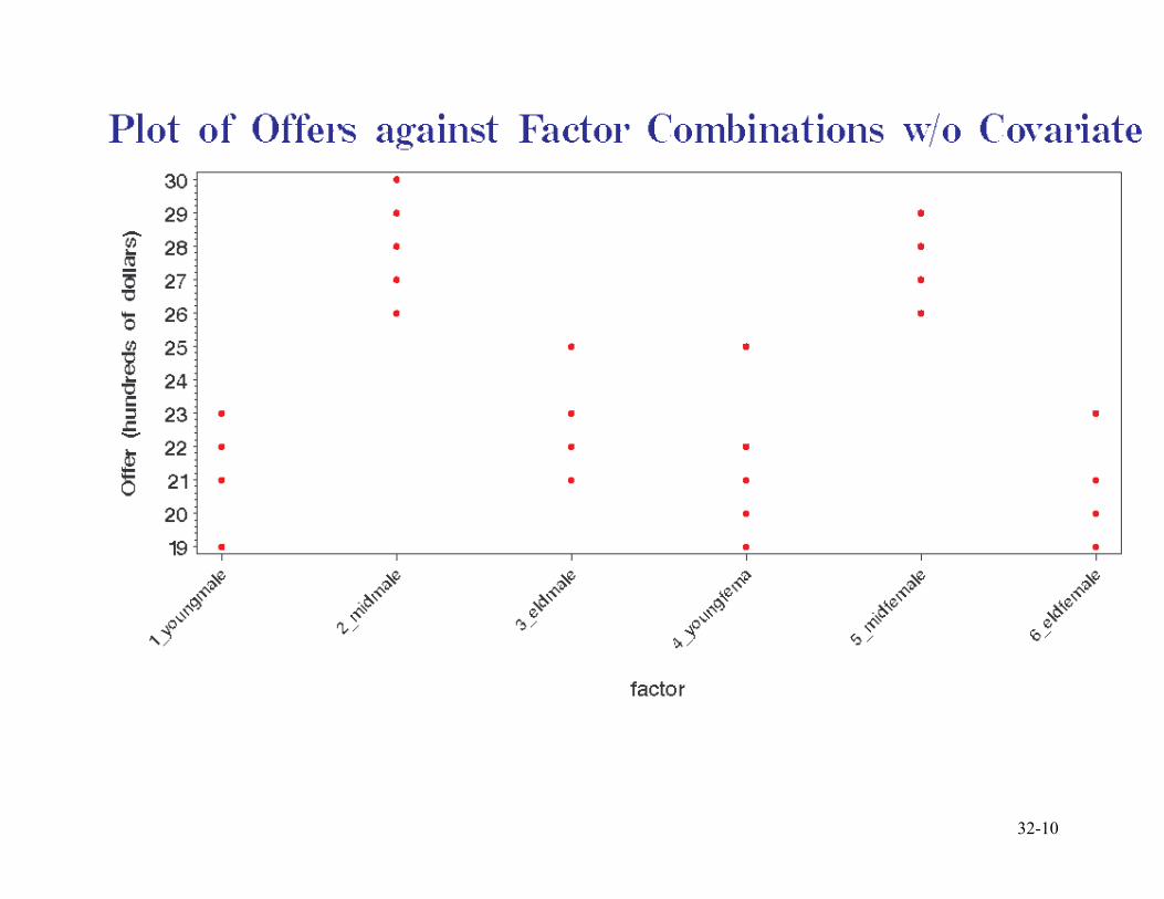
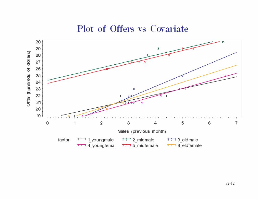
Two-way ANCOVA example

Cash Offers Example

(cashoffers_ancova.sas)

Y is offer made by a dealer on a used car

Factor 1 is the age of person selling the car

(young, middle, elderly)

Factor 2 is gender of the person selling the

car (male, female)

Covariate is overall sales volume for the

dealer

32-9

32-10

32-11

Plots w/o Covariate

Plots (and previous analysis) with simple

two-way ANOVA showed differences in

that middle-aged appeared to do better than

the other two groups; no interaction or

gender differences.

32-12

32-13

Covariate

Clearly is a relationship to the covariate;

higher sales means higher offers

Plot suggests a slight interaction; maybe

something different going on in the

elderly-male group.

Lets look at the ANCOVA

32-14

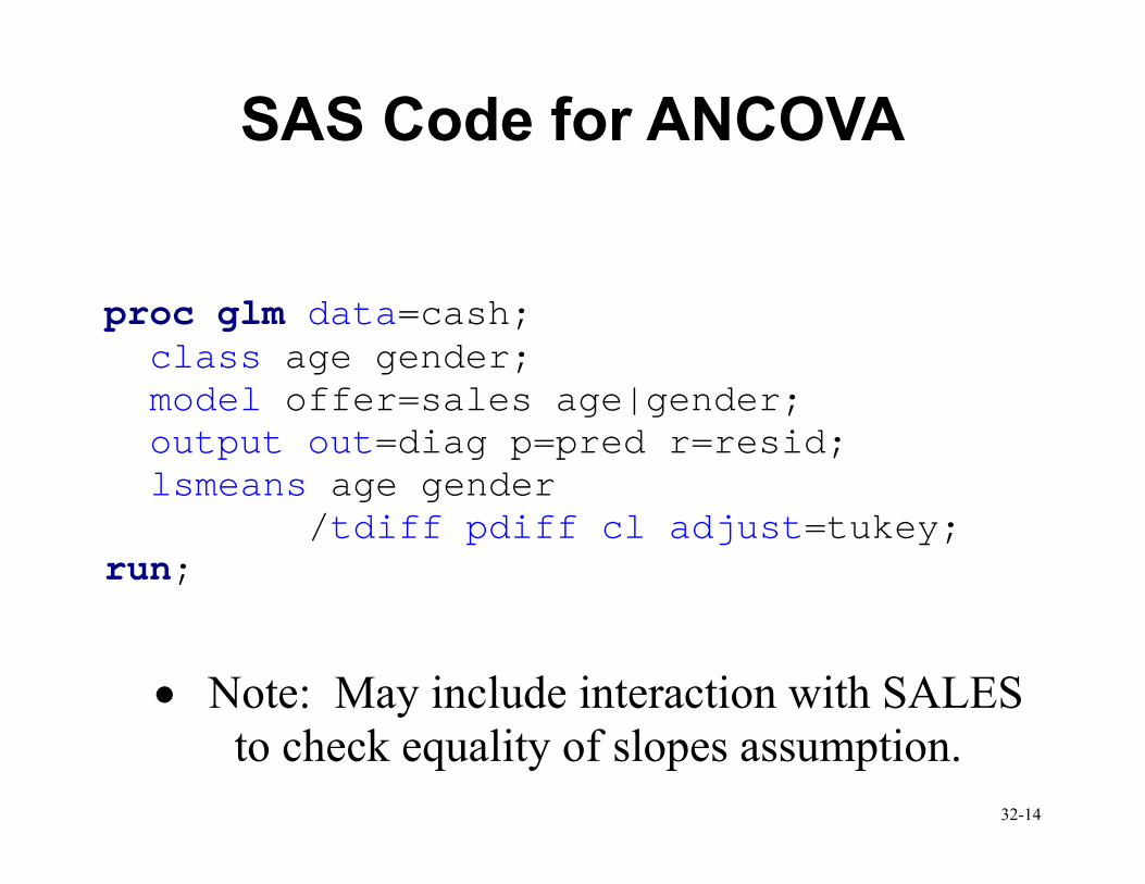
SAS Code for ANCOVA

proc glm data=cash; class age gender; model offer=sales age|gender; output out=diag p=pred r=resid;

lsmeans age gender /tdiff pdiff cl adjust=tukey;

run;

Note: May include interaction with SALES

to check equality of slopes assumption.

32-15

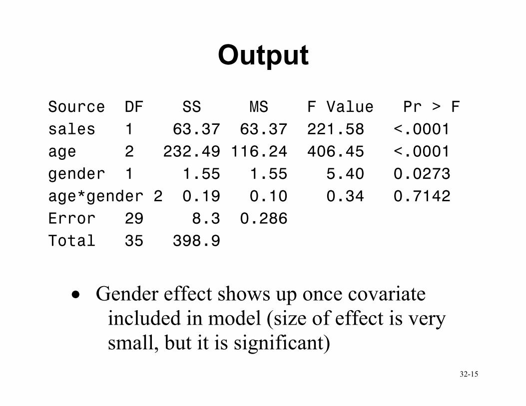
Output

Source DF SS MS F Value Pr > F

sales 1 63.37 63.37 221.58

32-16

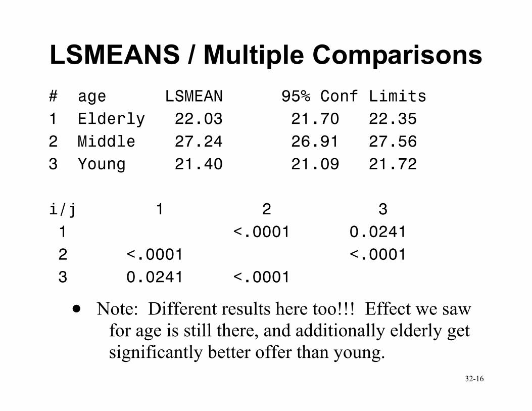
LSMEANS / Multiple Comparisons

# age LSMEAN 95% Conf Limits

1 Elderly 22.03 21.70 22.35

2 Middle 27.24 26.91 27.56

3 Young 21.40 21.09 21.72

i/j 1 2 3

1

32-17

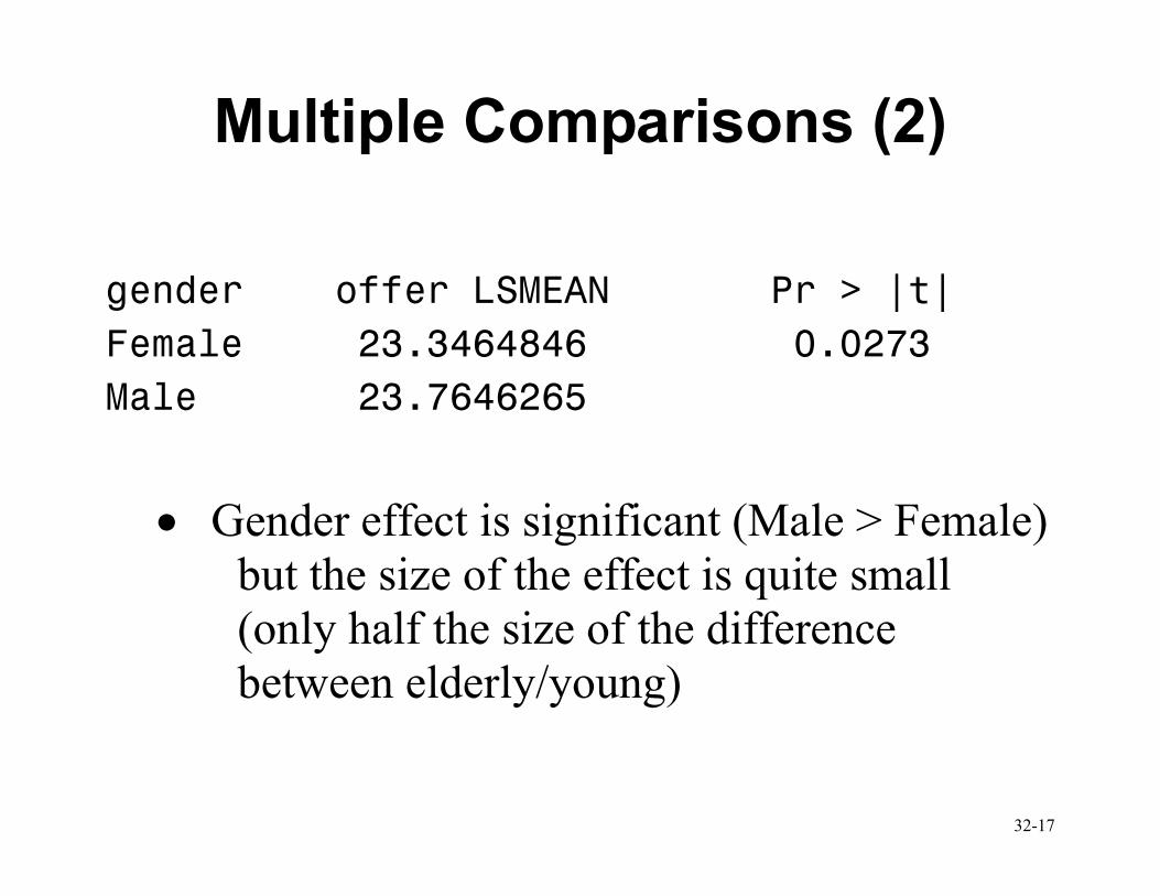
Multiple Comparisons (2)

gender offer LSMEAN Pr > |t|

Female 23.3464846 0.0273

Male 23.7646265

Gender effect is significant (Male > Female)

but the size of the effect is quite small

(only half the size of the difference

between elderly/young)

32-18

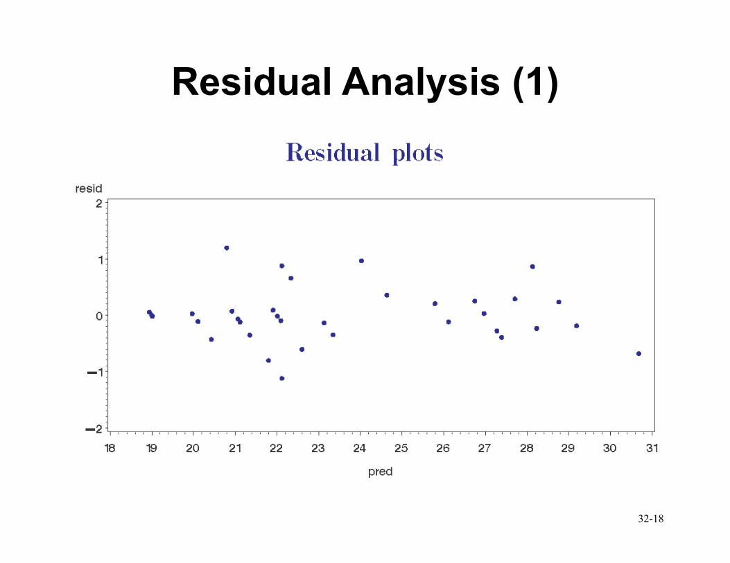
Residual Analysis (1)

32-19

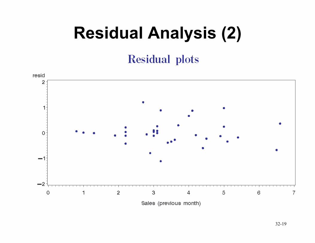
Residual Analysis (2)

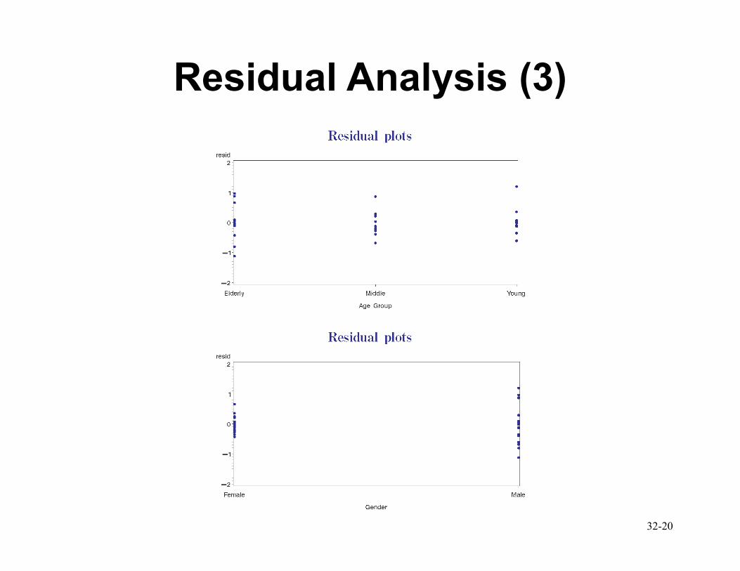
32-20

Residual Analysis (3)

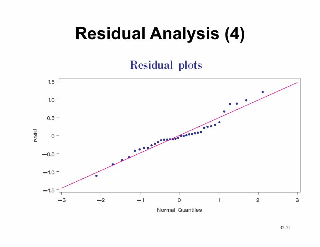
32-21

Residual Analysis (4)

32-22

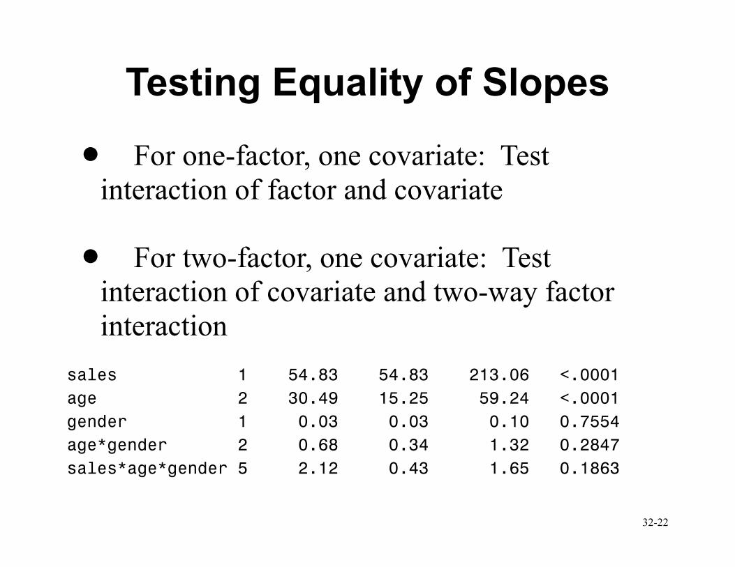
Testing Equality of Slopes

For one-factor, one covariate: Test interaction of factor and covariate

For two-factor, one covariate: Test interaction of covariate and two-way factor

interaction sales 1 54.83 54.83 213.06

32-23

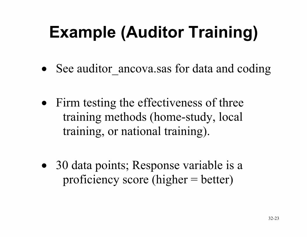
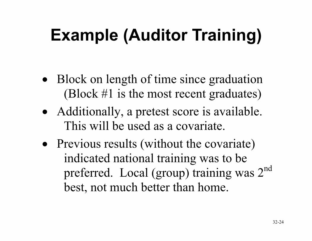
Example (Auditor Training)

See auditor_ancova.sas for data and coding

Firm testing the effectiveness of three

training methods (home-study, local

training, or national training).

30 data points; Response variable is a

proficiency score (higher = better)

32-24

Example (Auditor Training)

Block on length of time since graduation

(Block #1 is the most recent graduates)

Additionally, a pretest score is available.

This will be used as a covariate.

Previous results (without the covariate)

indicated national training was to be

preferred. Local (group) training was 2nd

best, not much better than home.

32-25

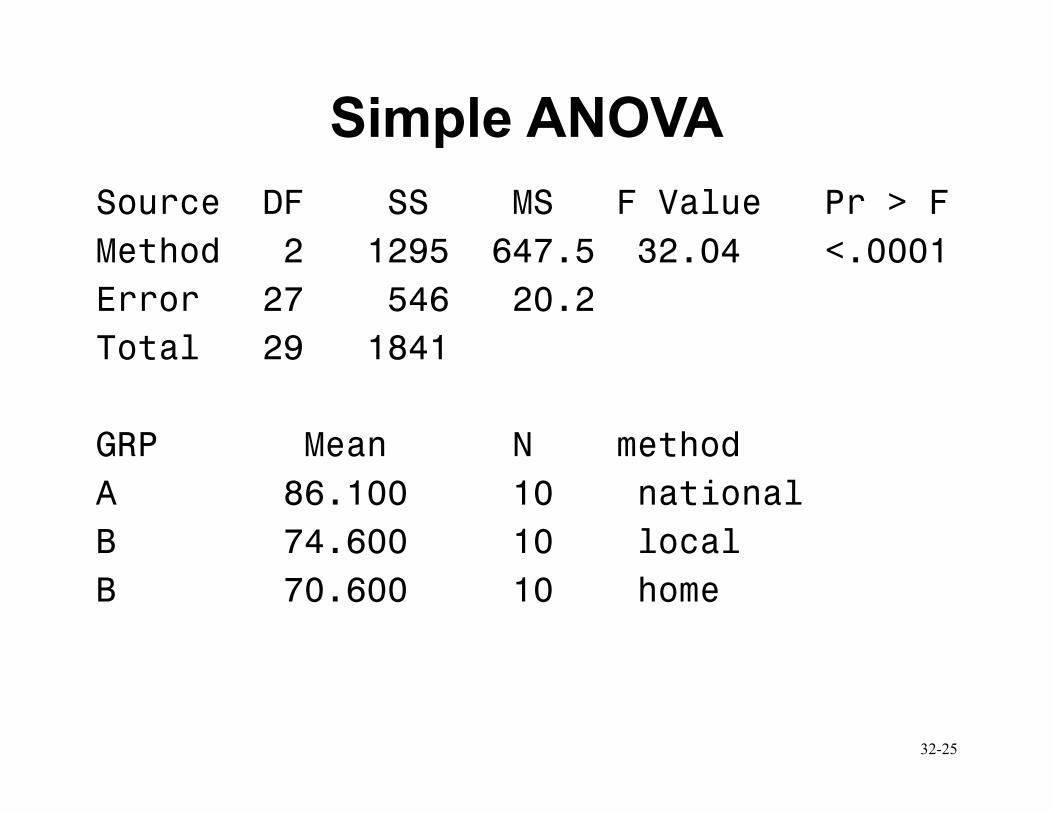
Simple ANOVA

Source DF SS MS F Value Pr > F

Method 2 1295 647.5 32.04

32-26

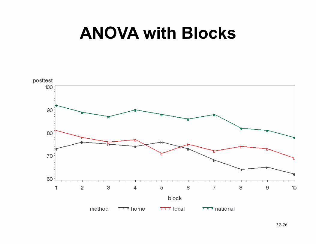
ANOVA with Blocks

32-27

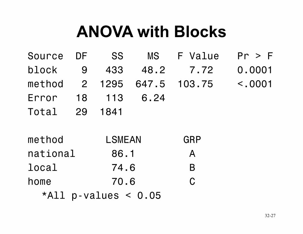
ANOVA with Blocks

Source DF SS MS F Value Pr > F

block 9 433 48.2 7.72 0.0001

method 2 1295 647.5 103.75

32-28

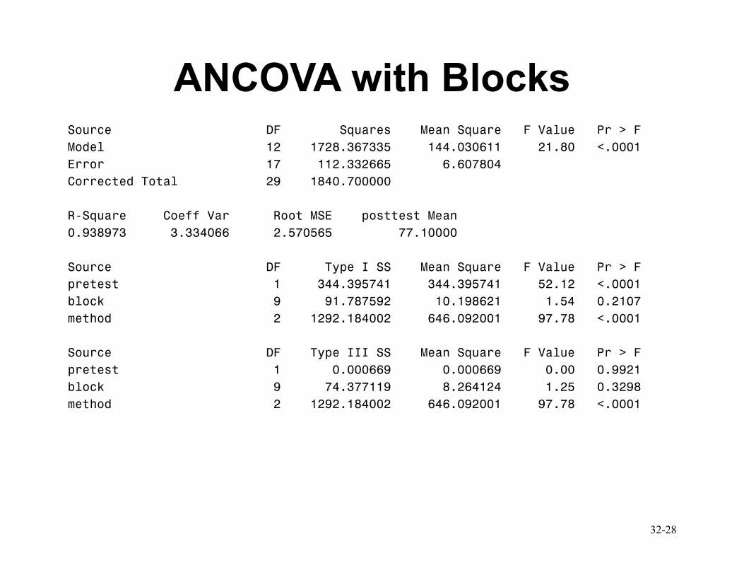
ANCOVA with Blocks Source DF Squares Mean Square F Value Pr > F

Model 12 1728.367335 144.030611 21.80 F

pretest 1 344.395741 344.395741 52.12

32-29

ANCOVA with Blocks

Type I SS : Pretest is significant alone, but

block is not significant in a model with pretest

(but we saw previously that it was significant

when pretest was not in the model).

Type III SS : Pretest and block are not

significant when other factors in model.

Method is significant when all other factors are

in the model.

32-30

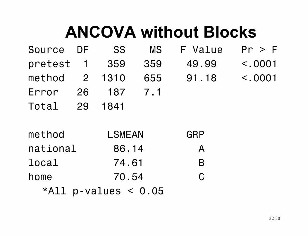
ANCOVA without Blocks Source DF SS MS F Value Pr > F

pretest 1 359 359 49.99

32-31

Summary of Results

In this case it turns out that you always will

identify the national training as the best.

Notice the slight differences in each analysis

we dont actually need both concomitant

variables (either use the block, or use the

pretest, the information is about the same).

32-32

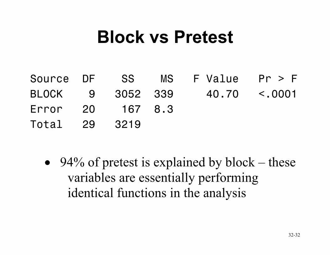
Block vs Pretest

Source DF SS MS F Value Pr > F

BLOCK 9 3052 339 40.70

32-33

Blocking vs. ANCOVA (1)

Sometimes researchers have a choice between

o CRD with covariance analysis (ANCOVA)

o RCBD with blocks formed by means of the concomitant variable

32-34

Blocking vs. ANCOVA (2)

If regression between response and

concomitant variable is linear, about equally

efficient. If not linear RCBD more effective.

RCBD are free of assumptions about the nature

of relationship between concomitant (blocking)

variable and response. ANCOVA assumes

linear relationship w/equal slopes between

groups.

RCBD may require more df for blocking

variable and thus leave less for the error.

32-35

Use of Differences For a posttest/prettest study, there are two

possible options for analysis:

o ANCOVA with posttest as response and prettest as a covariate

o ANOVA using difference (posttest-prettest) as the response.

If the slope parameter =1, then these

analyses are essentially equivalent.

If slope parameter is not near 1, then

ANCOVA may be more effective than the use

of differences.

32-36

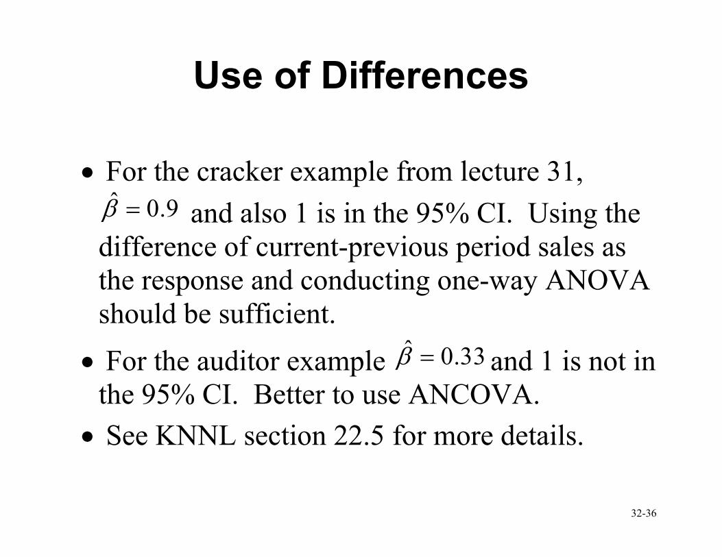
Use of Differences

For the cracker example from lecture 31,

0.9 = and also 1 is in the 95% CI. Using the

difference of current-previous period sales as

the response and conducting one-way ANOVA

should be sufficient.

For the auditor example 0.33 = and 1 is not in

the 95% CI. Better to use ANCOVA.

See KNNL section 22.5 for more details.

32-37

Upcoming...

Multi-Factor ANOVA (Chapter 24)