Differentially Private Covariance Estimation

Kareem Aminkamin@google.comGoogle Research NY

Travis Dicktdick@cs.cmu.edu

Carnegie Mellon University

Alex Kuleszakulesza@google.comGoogle Research NY

Andres Munoz Medinaammedina@google.com

Google Research NY

Sergei Vassilvitskiisergeiv@google.comGoogle Research NY

Abstract

The task of privately estimating a covariance matrix is a popular one due to itsapplications to regression and PCA. While there are known methods for releasingprivate covariance matrices, these algorithms either achive only (ε, δ)-differentialprivacy or require very complicated sampling schemes, ultimately performingpoorly in real data. In this work we propose a new ε-differentially private al-gorithm for computing the covariance matrix of a dataset that addresses both ofthese limitations. We show that it has lower error than existing state-of-the-artapproaches, both analytically and empirically. In addition, the algorithm is signif-icantly less complicated than other methods and can be efficiently implementedwith rejection sampling.

1 Introduction

Differential privacy has emerged as a standard framework for thinking about user privacy in thecontext of large scale data analysis [Dwork et al., 2014a]. While differential privacy does not protectagainst all attack vectors, it does provide formal guarantees about possible information leakage. Akey feature of differential privacy is its robustness to post-processing: once a mechanism is certifiedas differentially private, arbitrary post-processing can be performed on its outputs without additionalprivacy impact.

The past decade has seen the emergence of a wide range of techniques for modifying classicallearning algorithms to be differentially private [McSherry and Mironov, 2009, Chaudhuri et al.,2011, Jain et al., 2012, Abadi et al., 2016]. These algorithms typically train directly on the raw data,but inject carefully designed noise in order to produce differentially private outputs. A more general(and challenging) alternative approach is to first preprocess the dataset using a differentially privatemechanism and then freely choose among standard off-the-shelf algorithms for learning. This notonly provides more flexibility in the design of the learning system, but also removes the need foraccess to sensitive raw data (except for the initial preprocessing step). This approach thus fallsunder the umbrella of data release: since the preprocessed dataset is differentially private, it can, inprinciple, be released without leaking any individual’s data.

In this work we consider the problem of computing, in a differentially private manner, a specificpreprocessed representation of a dataset: its covariance matrix. Formally, given a data matrix X ∈Rd×n, where each column corresponds to a data point, we aim to compute a private estimate ofC = XX> that can be used in place of the raw data, for example, as the basis for standard linearregression algorithms. Our methods provide privacy guarantees for the columns of X.

There are many existing techniques that can be applied to this problem. We distinguish ε-differentially private algorithms, which promise what is sometimes referred to as pure differential

33rd Conference on Neural Information Processing Systems (NeurIPS 2019), Vancouver, Canada.

privacy, from (ε, δ)-differentially private algorithms, which may fail to preserve privacy with someprobability δ. While algorithms in the pure differential privacy setting give stronger privacy guaran-tees, they tend to be significantly more difficult to implement, and often underperform empiricallywhen compared to the straightforward algorithms in the (ε, δ) setting.

In this work, we give a new practical ε-differentially private algorithm for covariance matrix esti-mation. At a high level, the algorithm is natural. It approximates the eigendecomposition of thecovariance matrix C by estimating the collections of eigenvalues and eigenvectors separately. Sincethe eigenvalues are insensitive to changes in a single column of X, we can accurately estimate themusing the Laplace mechanism. To estimate the eigenvectors, the algorithm uses the exponentialmechanism to sample a direction θ from the unit sphere that approximately maximizes θ>Cθ, sub-ject to the constraint of being orthogonal to the approximate eigenvectors sampled so far. The overallprivacy guarantee for the combined method then follows from basic composition.

Our empirical results demonstrate lower reconstruction error for our algorithm when compared toother methods on both simulated and real-world datasets. This is especially striking in the high-privacy/low-ε regime, where we outperform all existing methods. We note that there is a differentregime where our bounds no longer compete with those of the Gaussian mechanism, namely when ε,δ, and the number of data points are all sufficiently large (i.e., when privacy is “easy”). This suggestsa two-pronged approach for the practitioner: utilize simple perturbation techniques when the datais insensitive to any one user and privacy parameters are lax, and more careful reconstruction whenthe privacy parameters are tight or the data is scarce, as is often the case in the social sciences andmedical research.

Our main results can be summarized as follows:

• We prove our algorithm improves the privacy/utility trade-off by achieving lower error ata given privacy parameter compared with previous pure differentially private approaches(Theorem 2).

• We derive a non-uniform allocation of the privacy budget for estimating the eigenvectors ofthe covariance matrix giving the strongest utility guarantee from our analysis (Corollary 1).

• We show that our algorithm is practical: a simple rejection sampling scheme can be usedfor the core of the implementation (Algorithm 2).

• Finally, we perform an empirical evaluation of our algorithm, comparing it to existing meth-ods on both synthetic and real-world datasets (Section 4). To the best of our knowledge,this is the first comparative empirical evaluation of different private covariance estimationmethods, and we show that our algorithm outperforms all of the baselines, especially in thehigh privacy regime.

1.1 Database Sanitization for Ridge Regression

Our motivation for private covariance estimation is training regression models. In practice, regres-sion models are trained using different subsets of features, multiple regularization parameters, andeven varying target variables. If we were to directly apply differentially private learning algorithmsfor each of these learning tasks, our privacy costs would accumulate with every model we trained.Our goal is to instead pay the privacy cost only once, computing a single data structure that can beused multiple times to tune regression models. In this section, we show that a private estimate ofthe covariance matrix C = XX> summarizes the data sufficiently well for all of these ridge regres-sion learning tasks with only a one-time privacy cost. Therefore, we can view differentially privatecovariance estimation as a database sanitization scheme for ridge regression.

Formally, given a data matrix X ∈ Rd×n with columns x1, . . . , xn, we denote the ith entry of xjby xj(i). Consider using ridge regression to learn a linear model for estimating some target featurex(t) as a function of x(−t), where x(−t) denotes the vector obtained by removing the tth featureof x ∈ Rd. That is, we want solve the following regularized optimization problem:

wα = argminw∈Rd−1

1

n

n∑j=1

1

2

(w>xj(−t)− xj(t)

)2+ α‖w‖22.

We can write the solution to the ridge regression problem in closed form as follows. Let A ∈R(d−1)×n be the matrix consisting all but the tth row of X and y =

(x1(t), . . . , xn(t)

)∈ Rn

2

be the tth row of X (as a column vector). Then the solution to the ridge regression problem withregularization parameter α is given by wα = (AA> + 2αnI)−1Ay.

Given access to just the covariance matrix C = XX>, we can compute the above closed form ridgeregression model. Suppose first that the target feature is t = d. Then, writing X in block-form, wehave

C = XX> =

[Ay>

] [A> y

]=

[AA> Ayy>A> y>y

].

Now it is not hard to see we can recover wα by using the block entries of the full covariance matrix.The following lemma quantifies how much the error of estimating C privately affects the regressionsolution wα. The proof can be found in Appendix A.

Lemma 1. Let X ∈ Rd×n be a data matrix, C = XX> ∈ Rd×d, and C ∈ Rd×d be a symmetricapproximation to C. Fix any target feature t and regularization parameter α. Let wα and wα be theridge regression models learned for predicting feature t from C and C, respectively. Then

‖wα − wα‖2 ≤‖C− C‖2,∞ + ‖C− C‖2 · ‖wα‖2

λmin(C) + 2αn,

where ‖M‖2,∞ denotes the L2,∞-norm of M (the maximum 2-norm of its columns).

Both ‖C−C‖2,∞ and ‖C−C‖2 are upper bounded by the Frobenius error ‖C−C‖F . Therefore, inour analysis of our differentially private covariance estimation mechanism, we will focus on bound-ing the Frobenius error. The bound in Lemma 1 also holds with ‖wα‖2 replaced by ‖wα‖2 in theright hand side, however we prefer the stated version since it can be computed by the practitioner.

1.2 Related Work

A variety of techniques exist for computing differentially private estimates of covariance matrices,including both general mechanisms that can be applied in this setting as well as specialized methodsthat take advantage of problem-specific structure.

A naıve approach using a standard differential privacy mechanism would be to simply add an ap-propriate amount of Laplace noise independently to every element in the true covariance matrix C.However, the amount of noise required makes such a mechanism impractical, as the sensitivity, andhence the amount of noise added, grows linearly in the dimension. A better approach is to addGaussian noise [Dwork et al., 2014b]; however, this results in (ε, δ)-differential privacy, where, withsome probability δ, the outcome is not private. Similarly, Upadhyay [2018] proposes a private wayof generating low dimensional representations of X. This is a slightly different task than covarianceestimation. Moreover, their algorithm is only (ε, δ)-differentially private for δ > n− logn whichmakes the privacy regime incomparable to the one proposed in this paper. Another approach, pro-posed in Chaudhuri et al. [2012], is to compute a private version of PCA. This approach has twolimitations. First, it only works for computing the top eigenvectors, and can fail to give non-trivialresults for computing the full covariance matrix. Second, the sampling itself is quite involved andrequires the use of a Gibbs sampler. Since it is generally impossible to know when the samplerconverges, adding noise in this manner can violate privacy guarantees.

The algorithm we propose bears the most resemblance to the differentially private low-rank matrixapproximation proposed by Kapralov and Talwar [2013], which approximates the SVD. Their al-gorithm computes a differentially private rank-1 approximation of a matrix C, subtracts this matrixfrom C and then iterates the process on the residual. Similarly, our approach iteratively generatesestimates of the eigenvectors of the matrix, but repeatedly projects the matrix onto the subspaceorthogonal to the previously estimated eigenvectors. We demonstrate the benefit of this projectiveupdate both in our analytical bounds and empirical results. This ultimately allows us to rely on asimple rejection sampling technique proposed by Kent et al. [2018] to select our eigenvectors.

Other perturbation approaches include recent work on estimating sparse covariance matrices byWang and Xu [2019]. Their setup differs from ours in that they assume all columns in the covariancematrix have s-sparsity. There was also an attempt by Jiang et al. [2016] to use Wishart-distributednoise to privately estimate a covariance matrix. However, Imtiaz and Sarwate [2016] proposed thesame algorithm and later discovered that the algorithm was in fact not differentially private.

3

Wang [2018] also study the effectiveness of differentially private covariance estimation for privatelinear regression (and compare against several other private regression approaches). However, theyonly consider the Laplace and Gaussian mechanisms for private covariance estimation and do notstudy the quality of the estimated covariance matrices, only their performance for regression tasks.

2 Preliminaries

Let X ∈ Rd×n be a data matrix where each column corresponds to a d-dimensional data point.Throughout the paper, we assume that the columns of the data matrix have `2-norm at most one1.Our goal is to privately release an estimate of the unnormalized and uncentered covariance matrixC = XX> ∈ Rd×d.

We say that two data matrices X and X are neighbors if they differ on at most one column, denotedby X ∼ X. We want algorithms that are ε-differentially private with respect to neighboring datamatrices. Formally, an algorithm A is ε-differentially private if for every pair of neighboring datamatrices X and X and every set O of possible outcomes, we have:

Pr(A(X) ∈ O) ≤ eε Pr(A(X) ∈ O) . (1)

A useful consequence of this definition is composability.Lemma 2. Suppose an algorithm A1 : Rd×n → Y1 is ε1-differentially private and a secondalgorithm A2 : Rd×n × Y1 → Y2 is ε2-differentially private. Then the composition A(X) =A2(X,A1(X)) is (ε1 + ε2)-differentially private.

Our main algorithm uses this property and multiple applications of the following mechanisms.

Laplace Mechanism. Let Lap(α) denote the Laplace distribution with parameter α. Given aquery f : Rd×n → Rk mapping data matrices to vectors, the `1-sensitivity of the query is given by∆f = maxX∼X ‖f(X)−f(X)‖1. For a given privacy parameter ε, the Laplace mechanism approx-imately answers queries by outputting f(X)+(Y1, . . . , Yk), where each Yi is independently sampledfrom the Lap(∆f/ε) distribution. The privacy and utility guarantees of the Laplace mechanism aresummarized in the following lemma.Lemma 3. The Laplace mechanism preserves ε-differential privacy and, for any β > 0, we havePr(maxi |Yi| ≥ ∆f

ε log kβ ) ≤ β.

Exponential Mechanism. The exponential mechanism can be used to privately select an approx-imately optimal outcome from an arbitrary domain. Formally, let (Y, µ) be a measure space andg : (X, y) 7→ g(X, y) be the utility of outcome y for data matrix X. The sensitivity of g is givenby ∆g = maxX∼X,y |g(X, y) − g(X, y)|. For ε > 0, the exponential mechanism samples y fromdensity proportional to fexp(y) = exp( ε

2∆gg(X, y)), defined with respect to the base measure µ.

Lemma 4 (McSherry and Talwar [2007]). The exponential mechanism preserves ε-differential pri-vacy. Let OPT = maxy g(X, y) and Gτ = y ∈ Y : g(X, y) ≥ OPT − τ. If y is the output ofthe exponential mechanism, we have Pr(y 6∈ G2τ ) ≤ exp

(−ετ/(2∆g)

)· µ(Gτ ).

In our algorithm, we will apply the exponential mechanism in order to choose unit-length approxi-mate eigenvectors. Therefore, the space of outcomes Y will be the unit sphere Sd−1 = θ ∈ Rd :‖θ‖2 = 1. For convenience, we will use the uniform distribution on the sphere, denoted by µ, asour base measure (this is proportional to the surface area). For example, the density p(θ) = 1 is theuniform distribution on Sd−1 and µ(Sd−1) = 1.

3 Iterative Eigenvalue Sampling for Covariance Estimation

In this section we describe our ε-differentially private covariance estimation mechanism. In fact, ourmethod produces a differentially private approximation to the eigendecomposition of C = XX>.

1If the columns of X have `2-norm bounded by a known value B, we can rescale the columns by 1/B toobtain a matrix X′ with column norm at most 1. Since XX> = B2X′X

′>, estimating the covariance matrixof X′ gives an estimate of the covariance matrix of X with Frobenius error inflated by a factor B2.

4

We first estimate the vector of eigenvalues, a query that has `1-sensitivity at most 2. Next, we showhow to use the exponential mechanism to approximate the top eigenvector of the covariance matrixC. Inductively, after estimating the top k eigenvectors θ1, . . . , θk of C, we project the data onto the(d− k)-dimensional orthogonal subspace and apply the exponential mechanism to approximate thetop eigenvector of the remaining projected covariance matrix. Once all eigenvalues and eigenvectorshave been estimated, the algorithm returns the reconstructed covariance matrix. Pseudocode for ourmethod is given in Algorithm 1. In Section 3.2 we discuss a rejection-sampling algorithm of Kentet al. [2018] that can be used for sampling the distribution defined in step (a) of Algorithm 1. Itis worth mentioning that if we only sample k eigenvectors, Algorithm 1 would return a rank k-approximation of matrix C.

Algorithm 1 Iterative Eigenvector SamplingInput: C = XX> ∈ Rd×d, privacy parameters ε0, . . . , εd.

1. Initialize C1 = C, P1 = I ∈ Rd×d, λi = λi(C) + Lap(2/ε0) for i = 1, . . . , d.2. For i = 1, . . . , d:

(a) Sample ui ∈ Sd−i proportional to fCi(u) = exp( εi4 u

>Ciu) and let θi = P>i ui.

(b) Find an orthonormal basis Pi+1 ∈ R(d−i)×d orthogonal to θ1, . . . , θi.(c) Let Ci+1 = Pi+1CP>i+1 ∈ R(d−i)×(d−i).

3. Output C =∑di=1 λiθiθ

>i .

Our approach is similar to the algorithm of Kapralov and Talwar [2013] with one significant differ-ence: in their algorithm, rather than projecting onto the orthogonal subspace of the first k estimatedeigenvectors, they subtract the rank-one matrix given by λiθiθ>i from C, where λi is the estimateof the ith eigenvalue. There are several advantages to using projections. First, the projection stepexactly eliminates the variance along the direction θi, while the rank-one subtraction will fail to doso if the estimated eigenvalues are incorrect (effectively causing us to pay for the eigenvalue ap-proximation twice: once in the reconstruction of the covariance matrix and once because it preventsus from removing the variance along the direction θi before estimating the remaining eigenvectors).Second, the analysis of the algorithm is substantially simplified because we are guaranteed that theestimated eigenvectors θ1, . . . , θd are orthogonal, and we do not require bounds for rank-one updateson the spectrum of a matrix.

We now show that Algorithm 1 is differentially private. The algorithm applies the Laplace mecha-nism once and the exponential mechanism d times, so the result follows from bounding the sensitiv-ity of the relevant queries and applying basic composition.

Theorem 1. Algorithm 1 preserves(∑d

i=0 εi)-differential privacy.

We now focus on the main contribution of this paper: a utility guarantee for Algorithm 1 in termsof the Frobenius distance between C and the true covariance matrix C as a function of the privacyparameters used for each step. An important consequence of this analysis is that we can optimizethe allocation of our total privacy budget ε among the d+ 1 queries in order to get the best bound.

First we provide a utility guarantee for the exponential mechanism applied to approximating the topeigenvector of a matrix C. This result is similar to the rank-one approximation guarantee given byKapralov and Talwar [2013], but we include a proof in the appendix for completeness.

Lemma 5. Let X ∈ Rd×n be a data matrix and C = XX>. For any β > 0, with probability atleast 1 − β over u sampled from the density proportional to fC(u) = exp( ε4u

>Cu) on Sd−1, wehave

u>Cu ≥ λ1(C)−O(

1

ε

(d log λ1(C) + log

1

β

))The following result characterizes the dependence of the Frobenius error on the errors in the es-timated eigenvalues and eigenvectors. In particular, given that the eigenvalue estimates all havebounded error, the dependence on the ith eigenvector estimate θi is only through the quantity

5

λi(C)− θ>i Cθi, which measures how much less variance of C is captured by θi as compared to thetrue ith eigenvector. Moreover, the contribution of θi is roughly weighted by λi. This observationallows us to tune the privacy budgeting across the d eigenvector queries, allocating more budget (atruntime) to the eigenvectors with large estimated eigenvalues. Empirically, we find that this budgetallocation step improves performance in some settings.

Lemma 6. Let C ∈ Rd×d be any positive semidefinite matrix. Let θ1, . . . , θd be any orthonormalvectors and λ1, . . . , λd be estimates of the eigenvalues of C satisfying |λi − λi(C)| ≤ τ for alli ∈ [d]. Then

‖C − ΘΛΘ>‖F ≤

√√√√2

d∑i=1

λi(C) · (λi(C)− θ>i Cθi) + τ√d

where Θ is the matrix with columns θi and Λ is the diagonal matrix with entries λi.

Proof. Let Λ ∈ Rd×d be the diagonal matrix of true eigenvalues of C. We have ‖C− ΘΛΘ>‖F ≤‖C− ΘΛΘ>‖F + ‖Θ(Λ− Λ)Θ>‖F . The second term is bounded by τ

√d, so it remains to bound

the first term. We have that

‖C− ΘΛΘ>‖2F = ‖C‖2F + ‖ΘΛΘ>‖2F − 2 tr(CΘΛΘ>) = 2∑i

λi(C)2 − 2∑i

λi(C)θ>i Cθi

= 2∑i

λi(C)(λi(C)− θ>i Cθi),

where the second equation follows from the fact that the first two terms are both equal to∑i λi(C)2

and the cyclic property of the trace. The final bound follows by taking the square root.

We are now ready to prove our main utility guarantee for Algorithm 1. The remaining analysisfocuses on the effect of working with the projected covariance matrices Ci. One interesting ob-servation is that our algorithm does not have error accumulating across its iterations due to theprojection step. Following Lemma 6, we only need to show that θi captures nearly as much of thevariance of C as the ith eigenvector. Fortunately, if our estimates θ1, . . . , θi−1 have errors, then theorthogonal subspace only contains more variance, and thus the sampling step in round i actuallybecomes easier. In this sense Algorithm 1 is “self-correcting”.

Theorem 2. Let C be the output of Algorithm 1 run with inputs C and privacy parametersε0, . . . , εd. For any β > 0, with probability at least 1− β we have

‖C− C‖F ≤ O(√√√√ d∑

i=1

dλi(C)

εi+

√d

ε0

),

where the O notation suppresses logarithmic terms in d, λ1(C), and β.

If Algorithm 1 is used to obtain a k-rank approximation, the above theorem can be modified to show

that the distance from the best k-rank approximation would be in O(√∑k

i=1dλi(C)εi

+√dε0

). Since

Theorem 2 bounds the error in terms of the privacy parameters ε0, . . . , εd, we can tune our allocationof the total privacy budget of ε across the d + 1 private operations in order to obtain the tightestpossible bound. In order to preserve privacy, we tune based on the estimated eigenvalues λ1, . . . , λdobtained in step (1) of Algorithm 1 rather than using the true eigenvalues. The following resultmakes precise the natural intuition that more effort should be made to estimate those eigenvectorswith larger (estimated) eigenvalues; its proof can be found in Appendix B.Corollary 1. Fix any privacy parameter ε and any failure probability β > 0, let ε0 = ε/2, and

let εi =ε2

√λi+τ∑

j

√λj+τ

where τ = 2ε0

log(2d/β). Then Algorithm 1 run with ε0, . . . , εd preserves

ε-differential privacy and, with probability at least 1− β, the output C satisfies

‖C− C‖F ≤ O(√

d

ε

d∑i=1

√λi +

1

ε+

√d

ε

).

6

3.1 Comparison of Bounds

In this section we compare the bound provided by Theorem 2 to previous state-of-the-art results.

Comparison to Kapralov and Talwar [2013]. The bounds given by Kapralov and Talwar [2013],when applied to the case of recovering the full-rank covariance matrix, bound the spectral error‖C − C‖2 by ζλ1(C) (for some ζ > 0) under the condition that λ1(C) is sufficiently large. Inparticular, Theorem 18 from their paper shows that there exists an ε-differentially private algorithmwith the above guarantee whenever λ1(C) ≥ C1d

4/(εζ6) for some constant C1. Since ‖C−C‖2 ≤‖C − C‖F , we can directly compare both algorithms after slightly rewriting our bounds. Thefollowing result shows that we improve the necessary lower bound on λ1(C) by a factor of d/ζ4

(ignoring log terms).

Corollary 2. For any ζ > 0 and any positive semidefinite matrix C, with probability at least0.99 (or any fixed success probability), running Algorithm 1 with ε0 = ε/2 and εi = ε/(2d) fori = 1, . . . , d preserves ε-differential privacy and outputs C such that ‖C − C‖F ≤ O(ζλ1(C)) ifλ1(C) ≥ 2d3

εζ2 log( dεζ ).

Comparison to Gaussian Mechanism. We can also directly compare to the error bounds for theGaussian mechanism given by Dwork et al. [2014b]. Theorem 9 in their paper gives ‖C − C‖F ≤O(d3/2

√log(1/δ)/ε), where ε and δ are the (approximate) differential privacy parameters. Using

privacy parameters ε0 = ε/2 and εi = ε/(2d) for i = 1, . . . , d, Theorem 2 implies that withhigh probability we have ‖C− C‖F ≤ O

(d3/2

√λ1(C) log(λ1(C))/ε +

√d/ε). For all values of

δ > 0, our algorithm provides a stronger privacy guarantee than the Gaussian mechanism. On theother hand, whenever λ1(C) log(λ1(C)) ≤ log(1/δ)/ε, our utility guarantee is tighter. Given thatλ1(C) = O(n), where n is the number of data points, we see that our algorithm admits better utilityguarantees in both the low data regime and the high privacy regime.

3.2 Sampling on the Sphere

To implement Algorithm 1, we need a subprocedure for drawing samples from the densities pro-portional to exp( ε4u

>Cu) defined on the sphere Sd−1, where C is a covariance matrix and ε is thedesired privacy parameter. This density belongs to a family called Bingham distributions. Kapralovand Talwar [2013] also discuss this sampling problem and, while their algorithm could also beused in our setting, we instead rely on a simpler rejection-sampling scheme proposed by Kent et al.[2018]. This sampling technique is exact and we find empirically that it is very efficient. Pseudocodefor their method is given in Algorithm 2 in the appendix.

Recall that rejection sampling allows us to generate samples from the distribution with density pro-portional to f , provided we can sample from the distribution with density proportional to a similarfunction g, called the envelope. Kent et al. [2018] propose to use the angular central Gaussiandistribution as an envelope. This distribution has a matrix parameter Ω and unnormalized density(defined on the sphere Sd−1) given by g(u) = (u>Ωu)−d/2. To sample from this distribution, wecan simply sample z from the mean-zero Gaussian distribution with covariance given by Ω−1 andoutput u = z/‖z‖2. Kent et al. [2018] provide a choice of parameter Ω to minimize the number ofrejected samples. They show that under some reasonable assumptions the expected number of rejec-tions grows like O(

√d) (see [Kent et al., 2018] for more details). In our experiments we observed

the median number of samples was less than d, and the mean was around 2d. We believe that ourempirical rejection counts are larger than the asymptotic bounds of Kent et al. [2018] because thedimensionality of our datasets is not large enough.

4 Experiments

We now present the results of an extensive empirical evaluation of the performance of our algorithm.Given a data matrix X, we study the performance of the algorithm on two tasks: (i) privately esti-mating the covariance matrix C = XX>, and (ii) privately regressing to predict one of the columnsof X from the others. Due to space constraints we present only the results of (i) and present theresults of (ii) in Appendix C.

7

10¡2 10¡1 100 101

²

0.0

0.5

1.0

1.5

2.0

2.5

3.0

Norm

aliz

ed e

rror

wined=13, n=200

AD IT-U L KT

10¡2 10¡1 100 101

²

0.0

0.2

0.4

0.6

0.8

1.0

1.2

airfoild=6,n=1.5K

10¡2 10¡1 100 101

²

0.00.51.01.52.02.53.03.54.0

adultd=108, n=49K

10¡2 10¡1 100 101

²

0.0

0.5

1.0

1.5

2.0

2.5

Norm

aliz

ed e

rror

wined=13, n=200

G-16 G-10 G-3 AD

10¡2 10¡1 100 101

²

0.0

0.2

0.4

0.6

0.8

1.0

1.2

airfoild=6,n=1.5K

10¡2 10¡1 100 101

²

0.00.20.40.60.81.01.21.41.61.8

adultd=108, n=49K

(a) (b)

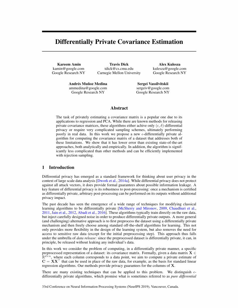
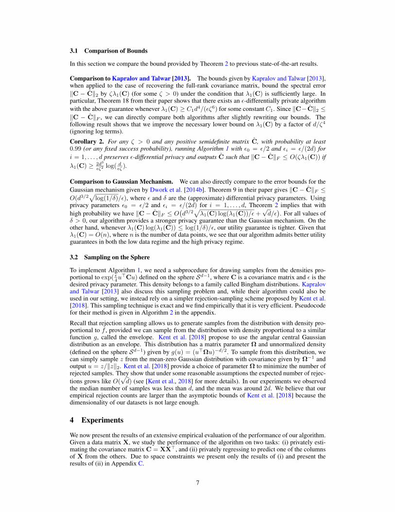
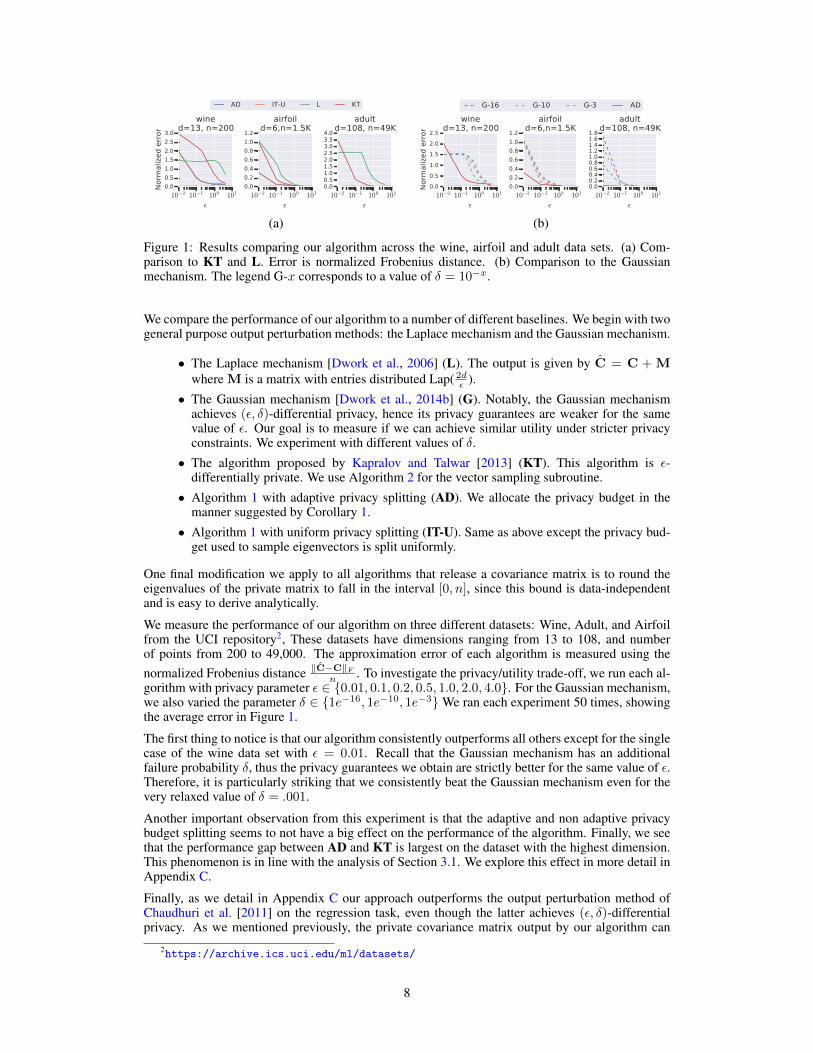
Figure 1: Results comparing our algorithm across the wine, airfoil and adult data sets. (a) Com-parison to KT and L. Error is normalized Frobenius distance. (b) Comparison to the Gaussianmechanism. The legend G-x corresponds to a value of δ = 10−x.

We compare the performance of our algorithm to a number of different baselines. We begin with twogeneral purpose output perturbation methods: the Laplace mechanism and the Gaussian mechanism.

• The Laplace mechanism [Dwork et al., 2006] (L). The output is given by C = C + Mwhere M is a matrix with entries distributed Lap( 2d

ε ).

• The Gaussian mechanism [Dwork et al., 2014b] (G). Notably, the Gaussian mechanismachieves (ε, δ)-differential privacy, hence its privacy guarantees are weaker for the samevalue of ε. Our goal is to measure if we can achieve similar utility under stricter privacyconstraints. We experiment with different values of δ.

• The algorithm proposed by Kapralov and Talwar [2013] (KT). This algorithm is ε-differentially private. We use Algorithm 2 for the vector sampling subroutine.

• Algorithm 1 with adaptive privacy splitting (AD). We allocate the privacy budget in themanner suggested by Corollary 1.

• Algorithm 1 with uniform privacy splitting (IT-U). Same as above except the privacy bud-get used to sample eigenvectors is split uniformly.

One final modification we apply to all algorithms that release a covariance matrix is to round theeigenvalues of the private matrix to fall in the interval [0, n], since this bound is data-independentand is easy to derive analytically.

We measure the performance of our algorithm on three different datasets: Wine, Adult, and Airfoilfrom the UCI repository2, These datasets have dimensions ranging from 13 to 108, and numberof points from 200 to 49,000. The approximation error of each algorithm is measured using thenormalized Frobenius distance ‖C−C‖F

n . To investigate the privacy/utility trade-off, we run each al-gorithm with privacy parameter ε ∈ 0.01, 0.1, 0.2, 0.5, 1.0, 2.0, 4.0. For the Gaussian mechanism,we also varied the parameter δ ∈ 1e−16, 1e−10, 1e−3We ran each experiment 50 times, showingthe average error in Figure 1.

The first thing to notice is that our algorithm consistently outperforms all others except for the singlecase of the wine data set with ε = 0.01. Recall that the Gaussian mechanism has an additionalfailure probability δ, thus the privacy guarantees we obtain are strictly better for the same value of ε.Therefore, it is particularly striking that we consistently beat the Gaussian mechanism even for thevery relaxed value of δ = .001.

Another important observation from this experiment is that the adaptive and non adaptive privacybudget splitting seems to not have a big effect on the performance of the algorithm. Finally, we seethat the performance gap between AD and KT is largest on the dataset with the highest dimension.This phenomenon is in line with the analysis of Section 3.1. We explore this effect in more detail inAppendix C.

Finally, as we detail in Appendix C our approach outperforms the output perturbation method ofChaudhuri et al. [2011] on the regression task, even though the latter achieves (ε, δ)-differentialprivacy. As we mentioned previously, the private covariance matrix output by our algorithm can

2https://archive.ics.uci.edu/ml/datasets/

8

be also be used to tune regularization parameters without affecting the privacy budget, thus givingadditional freedom to practitioners in tuning their algorithms.

5 Conclusion

We presented a new algorithm for differentially private covariance estimation, studied it analytically,and demonstrated its performance on a number of synthetic and real world datasets. To the best ofour knowledge this is the first ε-differentially private algorithm to admit a utility guarantee that growsas O(d3/2) with the dimension of the dataset. Previously, such bounds could only be achieved at thecost (ε, δ)-differential privacy. We also showed that the average Frobenius approximation error ofour algorithm decreases asO

(1√n

), which is slower than theO

(1n

)rate of the Gaussian and Laplace

mechanisms. This poses an open question of whether the suboptimal dependency on n is necessaryin order to achieve pure differential privacy or to achieve a dependency on the dimension ofO(d3/2).

Looking more broadly, practical machine learning and data analysis typically requires a significantamount of tuning: feature selection, hyperparameter selection, experimenting with regularization,and so on. If this tuning is performed using the underlying private dataset, then in principle all ofthese count against the privacy budget of the algorithm designer (who must also, of course, haveaccess to that private dataset). By producing a differentially private summary of the dataset fromwhich multiple models can be trained with no additional privacy cost, our approach allows a prac-titioner to operate freely, without worrying about privacy budgets or the secure handling of privatedata. We believe that finding techniques for computing private representations in other settings is anexciting direction for future research.

ReferencesMartin Abadi, Andy Chu, Ian Goodfellow, H Brendan McMahan, Ilya Mironov, Kunal Talwar, and

Li Zhang. Deep learning with differential privacy. In Proceedings of the 2016 ACM SIGSACConference on Computer and Communications Security, pages 308–318. ACM, 2016.

Keith Ball. An elementary introduction to modern convex geometry. Flavors of geometry, 31:1–58,1997.

K. Chaudhuri, A. Sarwate, and K. Sinha. Near-optimal algorithms for differentially-private principalcomponent analysis. In NIPS, 2012.

Kamalika Chaudhuri, Claire Monteleoni, and Anand D Sarwate. Differentially private empiricalrisk minimization. Journal of Machine Learning Research, 12(Mar):1069–1109, 2011.

Cynthia Dwork, Frank McSherry, Kobbi Nissim, and Adam D. Smith. Calibrating noise to sen-sitivity in private data analysis. In Third Theory of Cryptography Conference, pages 265–284,2006.

Cynthia Dwork, Aaron Roth, et al. The algorithmic foundations of differential privacy. Foundationsand Trends R© in Theoretical Computer Science, 9(3–4):211–407, 2014a.

Cynthia Dwork, Kunal Talwar, Abhradeep Thakurta, and Li Zhang. Analyze gauss: optimal boundsfor privacy-preserving principal component analysis. In Proceedings of the forty-sixth annualACM symposium on Theory of computing, pages 11–20. ACM, 2014b.

Hafiz Imtiaz and Anand D. Sarwate. Symmetric matrix perturbation for differentially-private princi-pal component analysis. In 2016 IEEE International Conference on Acoustics, Speech and SignalProcessing, ICASSP 2016, Shanghai, China, March 20-25, 2016, pages 2339–2343, 2016.

Prateek Jain, Pravesh Kothari, and Abhradeep Thakurta. Differentially private online learning. InConference on Learning Theory, pages 24–1, 2012.

Wuxuan Jiang, Cong Xie, and Zhihua Zhang. Wishart mechanism for differentially private principalcomponents analysis. In Proceedings of the Thirtieth AAAI Conference on Artificial Intelligence,February 12-17, 2016, Phoenix, Arizona, USA., pages 1730–1736, 2016.

9

Michael Kapralov and Kunal Talwar. On differentially private low rank approximation. In Proceed-ings of SODA, pages 1395–1414, 2013.

John T Kent, Asaad M Ganeiber, and Kanti V Mardia. A new unified approach for the simulation ofa wide class of directional distributions. Journal of Computational and Graphical Statistics, 27(2):291–301, 2018.

Daniel Kifer, Adam D. Smith, and Abhradeep Thakurta. Private convex optimization for empiricalrisk minimization with applications to high-dimensional regression. In Proceedings of COLT,pages 25.1–25.40, 2012.

F. McSherry and K. Talwar. Mechanism design via differential privacy. In FOCS, 2007.

Frank McSherry and Ilya Mironov. Differentially private recommender systems: Building privacyinto the netflix prize contenders. In Proceedings of the 15th ACM SIGKDD international confer-ence on Knowledge discovery and data mining, pages 627–636. ACM, 2009.

Jalaj Upadhyay. The price of privacy for low-rank factorization. In Proceedings of NeurIPS, pages4180–4191, 2018.

Di Wang and Jinhui Xu. Differentially private high dimensional sparse covariance matrix estimation.CoRR, abs/1901.06413, 2019. URL http://arxiv.org/abs/1901.06413.

Yu-Xiang Wang. Revisiting differentially private linear regression: optimal and adaptive prediction& estimation in unbounded domain. In Proceedings of UAI, 2018.

10

A Proofs for Regression Bounds

To simplify notation, we will let A(C, t) ∈ R(d−1)×n and b(C, t) ∈ Rn denote the blocks extractedfrom C so that the ridge regression model for predicting feature t with regularization parameter α isgiven by wα = (A(C, t) + 2αnI)−1b(C, t).

Lemma 1. Let X ∈ Rd×n be a data matrix, C = XX> ∈ Rd×d, and C ∈ Rd×d be a symmetricapproximation to C. Fix any target feature t and regularization parameter α. Let wα and wα be theridge regression models learned for predicting feature t from C and C, respectively. Then

‖wα − wα‖2 ≤‖C− C‖2,∞ + ‖C− C‖2 · ‖wα‖2

λmin(C) + 2αn,

where ‖M‖2,∞ denotes the L2,∞-norm of M (the maximum 2-norm of its columns).

Proof. First, we introduce some shorthand notation: let A = A(C, t), b = b(C, t), A = A(C, t),and b = b(C, t) be the blocks extracted from C and C so that (A + 2αnI)wα = b and (A +

2αnI)wλ = b. Subtracting the equalities defining wα and wα, we have

(A + 2αnI)wα − (A + 2αnI)wα = b− b.

Expanding the left hand side and adding and subtracting Awα, we have the following equivalences

(A + 2αnI)wα − (A + 2αnI)wα = b− b⇐⇒ Awα −Awα + Awα −Awα + 2αnI(wα − wα) = b− b⇐⇒ wα − wα = (A + 2αnI)−1

(b− b− (A−A)wα).

Therefore

‖wα − wα‖2 ≤ ‖(A + 2αnI)−1‖2(‖b− b‖2 + ‖A−A‖2 · ‖wα‖2

=‖b− b‖2 + ‖A−A‖2 · ‖wα‖2

λmin(A) + 2αn.

It remains to show that ‖b− b‖2 ≤ ‖C‖2,∞, ‖A−A‖2 ≤ ‖C−C‖2, and λmin(A) ≥ λmin(C).

First, since b and b correspond to the tth columns of C and C after removing the tth entries, we havethat ‖b− b‖2 ≤ ‖C−C‖2,∞.

The second two relations follow from the Cauchy interlacing theorem below, which allows us torelate the eigenvalues of a matrix M and any “principal sub-matrix”, which is a submatrix of Mobtained by repeatedly removing rows and columns with the same index.

Since A −A and A − A are a principal submatrices of C −C and C − C, respectively, we have‖A − A‖2 = maxλmax(A − A), λmax(A − A) ≤ maxλmax(C − C), λmax(C − C) =

‖C −C‖2, where the inequality follows from two applications of the interlacing theorem. Finally,since A is a principal submatrix of C, we have that λmin(A) ≥ λmin(C).

Theorem 3 (Cauchy Interlacing Theorem). Let M ∈ Rd×d be a symmetric matrix and N ∈ Rr×rbe a principal submatrix of M. Then for all j ≤ r, λj(M) ≤ λj(N) ≤ λd−r+j(M), where λj(M)denotes the jth smallest eigenvalue of M. In particular, if r = d− 1 then

λ1(M) ≤ λ1(N) ≤ · · · ≤ λd−1(M) ≤ λd−1(N) ≤ λd(M)

B Proofs for Iterative Covariance Estimation

We begin this section by formally proving that Algorithm 1 is private.

Theorem 1. Algorithm 1 preserves(∑d

i=0 εi)-differential privacy.

11

Proof. Let X = [Z;x] and X = [Z; x] be two neighboring data matrices in Rd×n with commoncolumns given by Z ∈ Rd×(n−1). For any matrix A, let Λ(A) = [λ1(A), . . . , λd(A)] denote thevector of eigenvalues of A. First, we argue that ‖Λ(ZZ>) − Λ(XX>)‖1 ≤ 1. For any vectorv ∈ Rd, we have v>XX>v = v>ZZ>v + v>xx>v ≥ v>ZZ>v. From this, it follows thatλi(XX>) ≥ λi(ZZ>) for all i ∈ [d]. Therefore, we have

‖Λ(XX>)− Λ(ZZ>)‖1 = tr(XX>)− tr(ZZ>) = tr(xx>) ≤ 1.

This bound also holds for XX>, so ‖Λ(XX>) − Λ(XX>)‖1 ≤ 2. Therefore, the instance of theLaplace mechanism in step (1) preserves ε0-differential privacy.

Next, for any matrix A, let g(A, θ) = θ>Aθ. For any direction θ ∈ Sd−1, we have

|g(XX>, θ)− g(XX>, θ)| = |θ>(xx> − xx>)θ| ≤ 2.

This bound also holds whenever we project the data into any subspace, so it follows that step (a) ofthe algorithm is using the exponential mechanism to maximize a utility function of sensitivity 2 andpreserves εi-differential privacy.

The final privacy guarantee follows by basic composition over the d+ 1 queries.

We now turn to the utility guarantees of this algorithm. Starting with the proof of Lemma 5. Webegin with a more precise bound on the probability that the exponential mechanism outputs a vectorthat captures τ less variance/energy of the covariance matrix C than the top eigenvector. In thisresult, we take advantage of the following lower bound on the µ-measure of a spherical cap:Lemma 7 (Lemma 2.3 of Ball [1997]). For any radius 0 ≤ r ≤ 2 and any center v ∈ Sd−1, wehave

µ(u ∈ Sd−1 : ‖v − u‖2 ≤ r

)≥ 1

2(r/2)d−1.

Lemma 8. Let X be any data matrix and C = XX>. Let u be a sample drawn from the distributionwith density proportional to fC(u) = exp( ε4u

>Cu) on Sd−1. For any τ > 0, we have

Pr(u>Cu ≤ λ1(C)− τ) ≤ 2 exp

(−τε

8

)(8λ1(C)

τ

)d−1

.

Proof. Define Gτ = u ∈ Sd−1 : u>Cu ≥ λ1(C) − τ to be the set of directions with atmost τ suboptimality. Applying the utility guarantee of Lemma 4, together with the fact that thesensitivity of g(X, u) = u>XX>u is 2 (see the proof of Theorem 1), we have that Pr(u 6∈ Gτ ) ≤exp( τε8 )/µ(Gτ/2). Our main arguments focus on lower bounding µ(Gτ/2).

Our strategy is to pick any direction u∗ ∈ argmaxu∈Sd−1 u>Cu and argue that all directions in aspherical cap of `2-radius r = τ

4λ1(C) around u∗ have utility at least λ1(C) − τ/2. It follows thatµ(Gτ/2) is at least the µ-measure of a spherical cap of `2 radius r = τ

4λ1(C) , which by Lemma 7

is at least 12 ( τ

8λ1(C) )d−1. Therefore, we have Pr(u 6∈ Gτ ) ≤ 2 exp(− τε8 )( 8λ1(C)τ )d−1, as required.

It remains to prove the following claim:

Claim. Let u∗ ∈ argmaxu∈Sd−1 u>Cu. Then for every u ∈ Sd−1 with ‖u − u∗‖2 ≤ τ4λ1(C) , we

have u>Cu ≥ λ1(C)− τ/2.

Proof. Let r = ‖u∗ − u‖2 be the distance between u∗ and u. We want to show that if r ≤ τ4λ1(C)

then u>Cu ≥ λ1(C) − τ/2. Let ‖ · ‖C be the induced seminorm (i.e., ‖v‖C =√v>Cv)). Then

we have that u>Cu = ‖u‖2C and√λ1(C) = ‖u∗‖C ≤ ‖u∗ − u‖C + ‖u‖C = ‖u∗ − u‖C +

√u>Cu,

which implies√u>Cu ≥

√λ1(C) − ‖u∗ − u‖C. Next, since ‖u∗ − u‖C =√

(u∗ − u)>C(u∗ − u) ≤ r√λ1(C), we have u>Cu ≥ (1 − r)2λ1(C) = λ1(C) + r2λ1(C) −

2rλ1(C) ≥ λ1(C) − 2rλ1(C). Therefore, if r ≤ τ4λ1(C) , we have 2rλ1(C) ≤ τ/2 and thus

u>Cu ≥ λ1(C)− τ/2.

12

All that remains to prove Lemma 5 is to choose an appropriate value of τ .Lemma 5. Let X ∈ Rd×n be a data matrix and C = XX>. For any β > 0, with probability atleast 1 − β over u sampled from the density proportional to fC(u) = exp( ε4u

>Cu) on Sd−1, wehave

u>Cu ≥ λ1(C)−O(

1

ε

(d log λ1(C) + log

1

β

))

Proof. The proof follows by setting τ = 8ε log

(e + 2(8λ1(C))d−1

β

)in Lemma 8. In particular, this

guarantees that with probability at least 1− β, we have

u>Cu ≥ λ1(C)− 8

εlog

(e+

2(8λ1(C))d−1

β

).

We can now prove the main utility guarantee of our algorithm.

Theorem 2. Let C be the output of Algorithm 1 run with inputs C and privacy parametersε0, . . . , εd. For any β > 0, with probability at least 1− β we have

‖C− C‖F ≤ O(√√√√ d∑

i=1

dλi(C)

εi+

√d

ε0

),

where the O notation suppresses logarithmic terms in d, λ1(C), and β.

Proof. First we bound the error in each of the differentially private estimations made by Algorithm 1.Let β′ = β/(2d). For each eigenvalue estimate, Lemma 3 guarantees that with probability at least1 − β/2, we have |λi − λi(C)| ≤ 2

ε0log 1

β′ . For each eigenvector estimate, Lemma 5 guaranteesthat with probability at least 1− β′ we have

λ1(Ci)− u>i Ciui ≤ O(

1

εi((d− i+ 1) log λ1(Ci) + log

1

β′)

). (2)

By the union bound, all events hold simultaneously with probability at least 1−β. Assume this highprobability event holds for the remainder of the proof.

The key remaining step is to argue that the guarantee from (2) implies that λi(C) − θ>i Cθi is alsosmall. First, let u ∈ Rd−i+1 be any unit vector and let θ = P>i u. Then we have ‖θ‖2 = 1 (since Pi

has orthonormal rows) and θ>Cθ = u>PiCP>i u = u>Ciu. Additionally, if a unit vector θ ∈ Rdcan be expressed as θ = P>i u, then ‖u‖2 = 1, and θ belongs to the (d−i+1)-dimensional subspacespanned by the rows of Pi. Thus, using the min-max characterization of λi(C) we have

λi(C) = minV⊂Rd

dim(V )=d−i+1

maxθ∈V‖θ‖2=1

θ>Cθ ≤ maxθ∈rowspan(Pi)‖θ‖2=1

θ>Cθ = maxu∈Rd−i+1

‖u‖2=1

u>Ciu = λ1(Ci).

This implies that

λi(C)− θ>i Cθi ≤ λ1(Ci)− u>i Ciui ≤ O(

1

εi(d log λ1(C) + log

1

β′)

),

where the final inequality uses (2) together with the fact that λ1(Ci) ≤ λ1(C). Combining withLemma 6, we have

‖C− C‖F ≤ O(√√√√ d∑

i=1

λi(C)(1

εi(d log λ1(C) + log

1

β′) +

√d log 1

β′

ε0

)

= O

(√√√√ d∑i=1

dλi(C)

εi+

√d

ε0

),

as required.

13

Next we prove the error bound for Algorithm 1 using the adaptive privacy budgeting.Corollary 1. Fix any privacy parameter ε and any failure probability β > 0, let ε0 = ε/2, and

let εi =ε2

√λi+τ∑

j

√λj+τ

where τ = 2ε0

log(2d/β). Then Algorithm 1 run with ε0, . . . , εd preserves

ε-differential privacy and, with probability at least 1− β, the output C satisfies

‖C− C‖F ≤ O(√

d

ε

d∑i=1

√λi +

1

ε+

√d

ε

).

Proof. With probability at least 1− β we are guaranteed that the high probability event from Theo-rem 2 occurs. In particular, we have that |λi − λi(C)| ≤ τ for all i and that

‖C− C‖F ≤ O(√√√√ d∑

i=1

dλi(C)

εi+

√d

ε0

).

Assume this high probability event holds for the remainder of the proof.

Given that λi(C) ≤ λi + τ and the above bound is increasing in λi(C), we can upper bound theloss in terms of the estimated eigenvalues as well:

‖C− C‖F ≤ O(√√√√ d∑

i=1

d(λi + τ)

εi+

√d

ε0

).

Substituing the given values for ε0, . . . , εd, this becomes

‖C− C‖F ≤ O(√√√√√ d∑

i=1

d(λi + τ) ·2∑j

√λj + τ

ε√λi + τ

+

√d

ε

)

= O

(√√√√d

ε

d∑i=1

√λi + τ

d∑j=1

√λj + τ +

√d

ε

)

= O

(√√√√d

ε

( d∑i=1

√λi + τ

)2

+

√d

ε

)

= O

(√d

ε

d∑i=1

√λi + τ +

√d

ε

),

as required.

Corollary 2. For any ζ > 0 and any positive semidefinite matrix C, with probability at least0.99 (or any fixed success probability), running Algorithm 1 with ε0 = ε/2 and εi = ε/(2d) fori = 1, . . . , d preserves ε-differential privacy and outputs C such that ‖C − C‖F ≤ O(ζλ1(C)) ifλ1(C) ≥ 2d3

εζ2 log( dεζ ).

Proof. From Theorem 2, we know that with probability at least 0.99 the output C of Algorithm 1satisfies

‖C− C‖F ≤ O(√√√√ d∑

i=1

dλi(C) log(λ1(C))

εi+

√d

ε0

).

Upper bounding λi(C) by λ1(C) and substituting the given privacy parameters ε0, . . . , εd, we have

‖C− C‖F ≤ O(d3/2

√λ1(C) log(λ1(C))/ε+

√d/ε)

≤ O(maxd3/2

√λ1(C) log(λ1(C))/ε,

√d/ε

)14

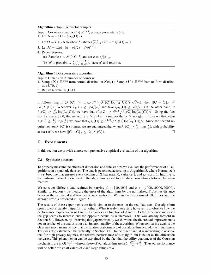
Algorithm 2 Top Eigenvector SamplerInput: Covariance matrix C ∈ Rd×d, privacy parameter ε > 0.1. Let A = − ε

4C + ε4λd(C) · I .

2. Let Ω = I + 2A/b where b satisfies∑di=1 1/(b+ 2λi(A)) = 0.

3. Let M = exp(−(d− b)/2) · (d/b)d/2.4. Repeat forever:

(a) Sample z ∼ N (0,Ω−1) and set u = z/‖z‖2.

(b) With probability exp(−u>Au)M ·(u>Ωu)d/2

‘accept’ and return u.

Algorithm 3 Data generating algorithmInput: Dimension d, number of points n.1. Sample X ∈ Rd×n from normal distribution N(0, 1). Sample U ∈ Rd×d from uniform distribu-

tion U(0, 1).2. Return Normalize(UX)

It follows that if ζλ1(C) ≥ maxd3/2√λ1(C) log(λ1(C))/ε,

√d/ε, then ‖C − C‖F ≤

O(ζλ1(C)). Whenever λ1(C) ≥√d/(εζ) we have ζλ1(C) ≥

√d/ε. On the other hand, if

λ1(C) ≥ d3

εζ2 log(λ1(C)), we have that ζλ1(C) ≥ d3/2√λ1(C) log(λ1(C))/ε. Using the fact

that for any a > 0, the inequality x ≥ 2a log(a) implies that x ≥ a log(x), it follows that whenλ1(C) ≥ 2d3

εζ2 log( dεζ ) we have that ζλ1(C) ≥ d3/2√λ1(C) log(λ1(C))/ε. Since the second re-

quirement on λ1(C) is stronger, we are guaranteed that when λ1(C) ≥ 2d3

εζ2 log( dεζ ), with probability

at least 0.99 we have ‖C− C‖F ≤ O(ζλ1(C)).

C Experiments

In this section we provide a more comprehensive empirical evaluation of our algorithm.

C.1 Synthetic datasets

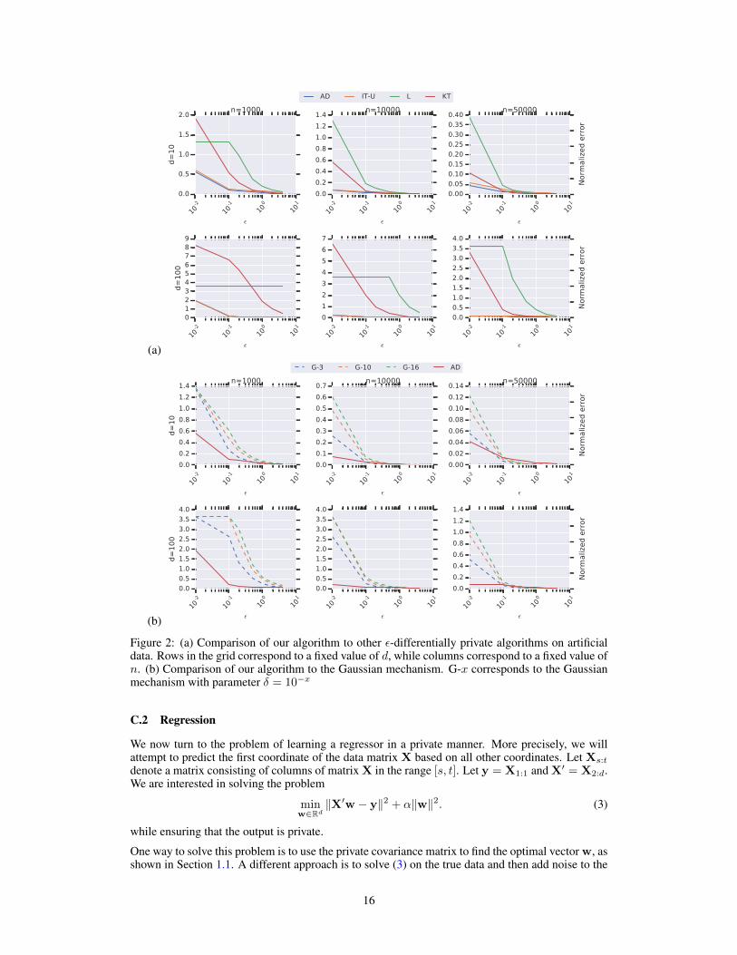
To properly measure the effects of dimension and data set size we evaluate the performance of all al-gorithms on a synthetic data set. The data is generated according to Algorithm 3, where Normalize()is a subroutine that ensures every column of X has mean 0, variance 1, and L2-norm 1. Intuitively,the uniform matrix U described in the algorithm is used to introduce correlations between betweenfeatures.

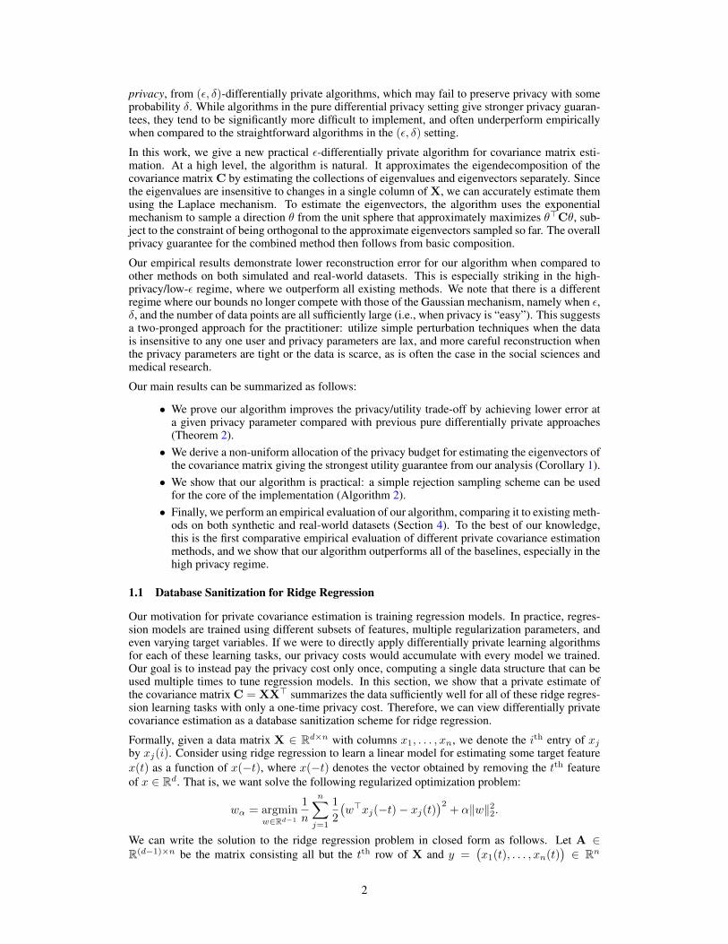
We consider different data regimes by varying d ∈ 10, 100 and n ∈ 1000, 10000, 50000.Similar to Section 4 we measure the error of the algorithms by the normalized Frobenius distancebetween the estimated and true covariance matrices. We ran each experiment 100 times and theaverage error is presented in Figure 2.

The results of these experiments are fairly similar to the ones on the real data sets. Our algorihtmseems to consistently outperform all others. What is truly interesting however is to observe how theperformance gap between AD and KT changes as a function of d and n. As the dimension increasesthe gap seems to increase and the opposite occurs as n increases. This was already foretold inSection 3.1. However, by observing this gap empirically we show that the theoretical improvement isnot an artifact of the analysis but a an inherent quality of the algorithm. When comparing against theGaussian mechanism we see that the relative performance of our algorithm degrades as n increases.This was also established theoretically in Section 3.1. On the other hand, it is interesting to observethat for high privacy regimes, the relative performance of our algorithm is better as the dimensionincreases. This phenomenon can be explained by the fact that the utility guarantees of the Gaussianmechanism are inO(d

3/2

ε ) whereas those of our algorithm are inO(d3/2√ε

+ dε ). Thus our performance

will be better for small values of ε and large values of d.

15

(a)

10-2

10-1

100

101

²

0.0

0.5

1.0

1.5

2.0

d=

10

n=1000

AD IT-U L KT

10-2

10-1

100

101

²

0.0

0.2

0.4

0.6

0.8

1.0

1.2

1.4n=10000

10-2

10-1

100

101

²

0.00

0.05

0.10

0.15

0.20

0.25

0.30

0.35

0.40n=50000

Norm

aliz

ed e

rror

10-2

10-1

100

101

²

0123456789

d=

10

0

10-2

10-1

100

101

²

0

1

2

3

4

5

6

7

10-2

10-1

100

101

²

0.0

0.5

1.0

1.5

2.0

2.5

3.0

3.5

4.0

Norm

aliz

ed e

rror

(b)

10-2

10-1

100

101

²

0.0

0.2

0.4

0.6

0.8

1.0

1.2

1.4

d=

10

n=1000

G-3 G-10 G-16 AD

10-2

10-1

100

101

²

0.0

0.1

0.2

0.3

0.4

0.5

0.6

0.7n=10000

10-2

10-1

100

101

²

0.00

0.02

0.04

0.06

0.08

0.10

0.12

0.14n=50000

Norm

aliz

ed e

rror

10-2

10-1

100

101

²

0.0

0.5

1.0

1.5

2.0

2.5

3.0

3.5

4.0

d=

10

0

10-2

10-1

100

101

²

0.0

0.5

1.0

1.5

2.0

2.5

3.0

3.5

4.0

10-2

10-1

100

101

²

0.0

0.2

0.4

0.6

0.8

1.0

1.2

1.4

Norm

aliz

ed e

rror

Figure 2: (a) Comparison of our algorithm to other ε-differentially private algorithms on artificialdata. Rows in the grid correspond to a fixed value of d, while columns correspond to a fixed value ofn. (b) Comparison of our algorithm to the Gaussian mechanism. G-x corresponds to the Gaussianmechanism with parameter δ = 10−x

C.2 Regression

We now turn to the problem of learning a regressor in a private manner. More precisely, we willattempt to predict the first coordinate of the data matrix X based on all other coordinates. Let Xs:t

denote a matrix consisting of columns of matrix X in the range [s, t]. Let y = X1:1 and X′ = X2:d.We are interested in solving the problem

minw∈Rd

‖X′w − y‖2 + α‖w‖2. (3)

while ensuring that the output is private.

One way to solve this problem is to use the private covariance matrix to find the optimal vector w, asshown in Section 1.1. A different approach is to solve (3) on the true data and then add noise to the

16

10-2

10-1

100

101

²

10-1

100

d=

10

n=1000

AD-1.0

AD-10.0

AD-100.0

AD-1000.0

P-10.0

P-100.0

P-1000.0

10-2

10-1

100

101

²

10-2

10-1 n=10000

10-2

10-1

100

101

²

10-3

10-2

10-1 n=50000

Square

loss

10-2

10-1

100

101

²

10-2

10-1

100

d=

10

0

10-2

10-1

100

101

²

10-3

10-2

10-1

10-2

10-1

100

101

²

10-4

10-3

10-2

10-1

Square

loss

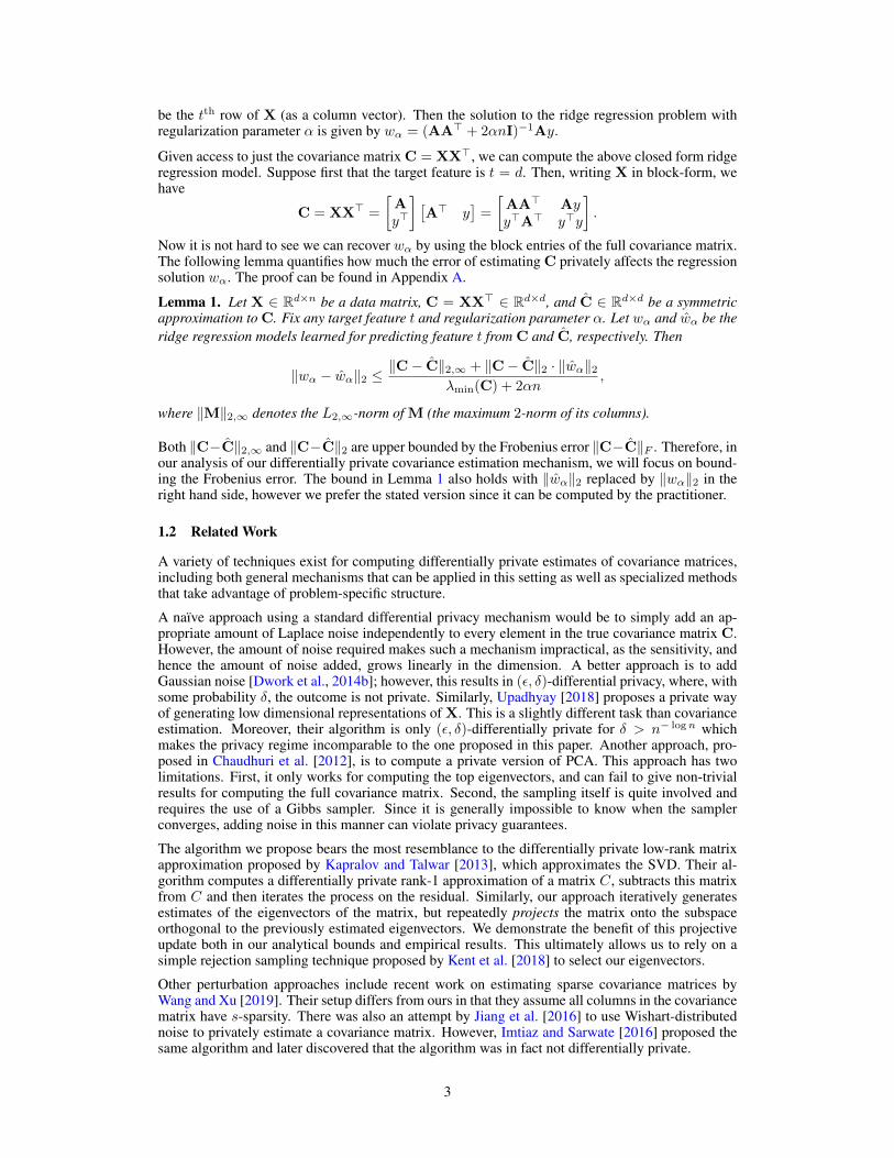
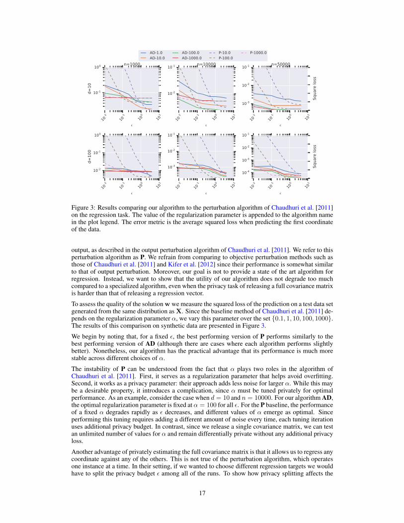
Figure 3: Results comparing our algorithm to the perturbation algorithm of Chaudhuri et al. [2011]on the regression task. The value of the regularization parameter is appended to the algorithm namein the plot legend. The error metric is the average squared loss when predicting the first coordinateof the data.

output, as described in the output perturbation algorithm of Chaudhuri et al. [2011]. We refer to thisperturbation algorithm as P. We refrain from comparing to objective perturbation methods such asthose of Chaudhuri et al. [2011] and Kifer et al. [2012] since their performance is somewhat similarto that of output perturbation. Moreover, our goal is not to provide a state of the art algorithm forregression. Instead, we want to show that the utility of our algorithm does not degrade too muchcompared to a specialized algorithm, even when the privacy task of releasing a full covariance matrixis harder than that of releasing a regression vector.

To assess the quality of the solution w we measure the squared loss of the prediction on a test data setgenerated from the same distribution as X. Since the baseline method of Chaudhuri et al. [2011] de-pends on the regularization parameter α, we vary this parameter over the set 0.1, 1, 10, 100, 1000.The results of this comparison on synthetic data are presented in Figure 3.

We begin by noting that, for a fixed ε, the best performing version of P performs similarly to thebest performing version of AD (although there are cases where each algorithm performs slightlybetter). Nonetheless, our algorithm has the practical advantage that its performance is much morestable across different choices of α.

The instability of P can be understood from the fact that α plays two roles in the algorithm ofChaudhuri et al. [2011]. First, it serves as a regularization parameter that helps avoid overfitting.Second, it works as a privacy parameter: their approach adds less noise for larger α. While this maybe a desirable property, it introduces a complication, since α must be tuned privately for optimalperformance. As an example, consider the case when d = 10 and n = 10000. For our algorithm AD,the optimal regularization parameter is fixed at α = 100 for all ε. For the P baseline, the performanceof a fixed α degrades rapidly as ε decreases, and different values of α emerge as optimal. Sinceperforming this tuning requires adding a different amount of noise every time, each tuning iterationuses additional privacy budget. In contrast, since we release a single covariance matrix, we can testan unlimited number of values for α and remain differentially private without any additional privacyloss.

Another advantage of privately estimating the full covariance matrix is that it allows us to regress anycoordinate against any of the others. This is not true of the perturbation algorithm, which operatesone instance at a time. In their setting, if we wanted to choose different regression targets we wouldhave to split the privacy budget ε among all of the runs. To show how privacy splitting affects the

17

10-2

10-1

100

101

²

10-1

100

d=

10

n=1000

AD-1.0

AD-10.0

AD-100.0

AD-1000.0

P-10.0

P-100.0

P-1000.0

10-2

10-1

100

101

²

10-2

10-1 n=10000

10-2

10-1

100

101

²

10-3

10-2

10-1 n=50000

Avg S

quare

loss

10-2

10-1

100

101

²

10-2

10-1

100

d=

10

0

10-2

10-1

100

101

²

10-3

10-2

10-1

10-2

10-1

100

101

²

10-4

10-3

10-2

10-1

Avg S

quare

loss

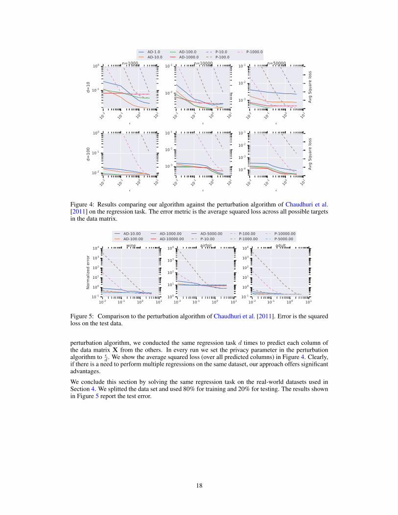
Figure 4: Results comparing our algorithm against the perturbation algorithm of Chaudhuri et al.[2011] on the regression task. The error metric is the average squared loss across all possible targetsin the data matrix.

10-2 10-1 100 10110-1

100

101

102

103

104

Norm

aliz

ed e

rror

wine

AD-10.00

AD-100.00

AD-1000.00

AD-10000.00

AD-5000.00

P-10.00

P-100.00

P-1000.00

P-10000.00

P-5000.00

10-2 10-1 100 101100

101

102

103

104 airfoil

10-2 10-1 100 10110-1

100

101

102

103

104 adult

Figure 5: Comparison to the perturbation algorithm of Chaudhuri et al. [2011]. Error is the squaredloss on the test data.

perturbation algorithm, we conducted the same regression task d times to predict each column ofthe data matrix X from the others. In every run we set the privacy parameter in the perturbationalgorithm to ε

d . We show the average squared loss (over all predicted columns) in Figure 4. Clearly,if there is a need to perform multiple regressions on the same dataset, our approach offers significantadvantages.

We conclude this section by solving the same regression task on the real-world datasets used inSection 4. We splitted the data set and used 80% for training and 20% for testing. The results shownin Figure 5 report the test error.

18