Ilya L. Shapiro
Theoretisch-Physikalisches Institut
Lecture 2.
Local momentum representation. Covariance.
Renormalization group.
In curved space the Effective Action (EA) depends on metric
Γ[Φ] → Γ[Φ, gµν ] .
Feynman diagrams: one has to consider grafs with internal lines of matter fields and external limes of both matter and metric. In practice, one can consider gµν = ηµν + hµν .
Is it possible to get EA for an arbitrary background in this way? Perhaps not. But it is sufficient to explore renormalization!
An important aspect is that the general covariance in the non-covariant gauges can be shown in the framework of mathematically rigid Batalin-Vilkovisky quantization scheme:
• P. Lavrov and I.Sh., Phys. Rev. D81 (2010).
Strong arguments supporting locality of the counterterms follow from the “quantum gravity completion” consideration.
Still, it would be very nice to have an explicitly covariant method of deriving counterterms at all loop orders.
Ilya Shapiro, Lectures on curved-space QFT, February - 2012
Riemann normal coordinates.
Consider the manifold M3,1 and choose some point with the coordinates x ′µ. The normal coordinates yµ = xµ − x ′µ satisfy several conditions.
The lines of constant coordinates are geodesics which are completely defined by the tangent vectors
ξµ = dxµ
x ′ , τ(x ′) = 0
and τ is natural parameter along the geodesic. Moreover, we request that metric at the point x ′ be the Minkowski one ηµν . For an arbitrary function A(x)
A(x ′ + y) = A′ + ∂A ∂yα
yα + 1 2
∂2A ∂yα∂yβ
Ilya Shapiro, Lectures on curved-space QFT, February - 2012
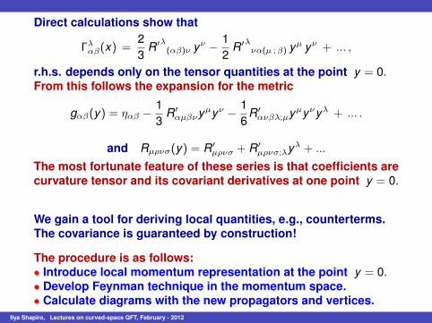
Direct calculations show that
2 R′λ
να(µ ;β) yµ yν + ... ,
r.h.s. depends only on the tensor quantities at the point y = 0. From this follows the expansion for the metric
gαβ(y) = ηαβ − 1 3
µρνσ;λyλ + ...
The most fortunate feature of these series is that coefficients are curvature tensor and its covariant derivatives at one point y = 0.
We gain a tool for deriving local quantities, e.g., counterterms. The covariance is guaranteed by construction!
The procedure is as follows: • Introduce local momentum representation at the point y = 0. • Develop Feynman technique in the momentum space. • Calculate diagrams with the new propagators and vertices.
Ilya Shapiro, Lectures on curved-space QFT, February - 2012
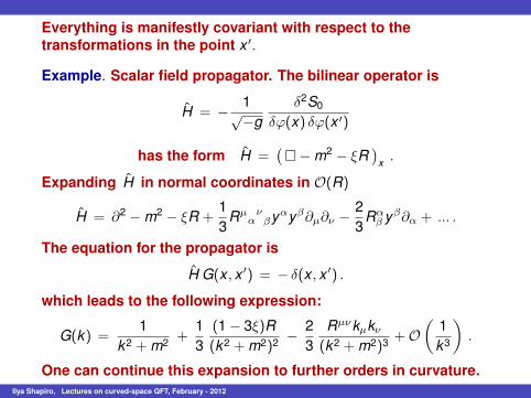
Everything is manifestly covariant with respect to the transformations in the point x ′.
Example. Scalar field propagator. The bilinear operator is
H = − 1√ −g
) x .
H = ∂2 − m2 − ξR + 1 3
Rµ α ν βyαyβ∂µ∂ν − 2
3 Rα
H G(x , x ′) = − δ(x , x ′) .
which leads to the following expression:
G(k) = 1
( 1 k3
) .
One can continue this expansion to further orders in curvature. Ilya Shapiro, Lectures on curved-space QFT, February - 2012
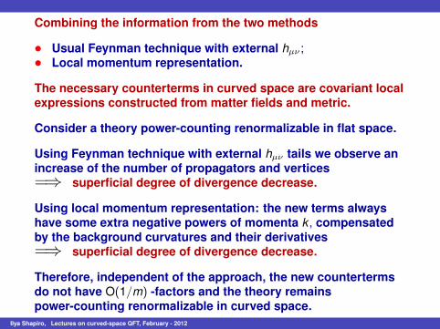
Combining the information from the two methods
• Usual Feynman technique with external hµν ; • Local momentum representation.
The necessary counterterms in curved space are covariant local expressions constructed from matter fields and metric.
Consider a theory power-counting renormalizable in flat space.
Using Feynman technique with external hµν tails we observe an increase of the number of propagators and vertices =⇒ superficial degree of divergence decrease.
Using local momentum representation: the new terms always have some extra negative powers of momenta k , compensated by the background curvatures and their derivatives =⇒ superficial degree of divergence decrease.
Therefore, independent of the approach, the new counterterms do not have O(1/m) -factors and the theory remains power-counting renormalizable in curved space.
Ilya Shapiro, Lectures on curved-space QFT, February - 2012
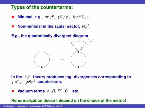
Types of the counterterms:
E.g., the quadratically divergent diagram
=⇒
in the λφ4 theory produces log. divergences corresponding to∫ d4√−gRφ2 counterterm.
• Vacuum terms Λ, R, R2, C2, etc.
Renormalization doesn’t depend on the choice of the metric! Ilya Shapiro, Lectures on curved-space QFT, February - 2012
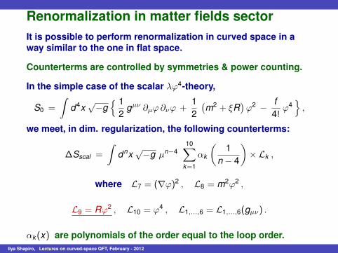
Renormalization in matter fields sector It is possible to perform renormalization in curved space in a way similar to the one in flat space.
Counterterms are controlled by symmetries & power counting.
In the simple case of the scalar λφ4-theory,
S0 =
∫ d4x
√ −g
( m2 + ξR
) φ2 − f
4! φ4
Sscal =
∫ dnx
L9 = Rφ2 , L10 = φ4 , L1,...,6 = L1,...,6(gµν) .
αk (x) are polynomials of the order equal to the loop order. Ilya Shapiro, Lectures on curved-space QFT, February - 2012
The situation is similar for any theory which is renormalizable in flat space: only ξRφ2 counterterms represent a new element in the matter sector.
Moreover, due to covariance, multiplicative renormalization factors, e.g., Z1, in
φ0 = µ n−4
are exactly the same as in the flat space.
The renormalization relations for the scalar mass m and nonminimal parameter ξ have the form
m2 0 = Z2 m2 , ξ0 −
1 6 = Z2
Z2 = Z2 , Z3 = 0 .
So, in principle, we even do not need to perform a special calculation of renormalization for ξ at the 1-loop order.
Ilya Shapiro, Lectures on curved-space QFT, February - 2012
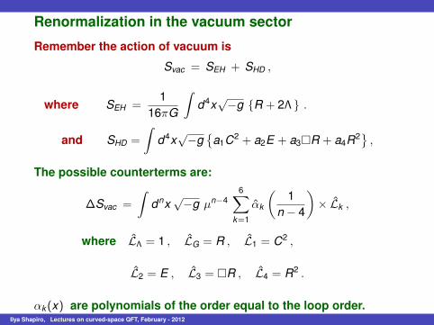
Renormalization in the vacuum sector
Remember the action of vacuum is
Svac = SEH + SHD ,
where SEH = 1
The possible counterterms are:
L2 = E , L3 = R , L4 = R2 .
αk (x) are polynomials of the order equal to the loop order. Ilya Shapiro, Lectures on curved-space QFT, February - 2012
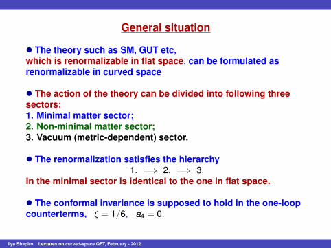
General situation
• The theory such as SM, GUT etc, which is renormalizable in flat space, can be formulated as renormalizable in curved space
• The action of the theory can be divided into following three sectors: 1. Minimal matter sector; 2. Non-minimal matter sector; 3. Vacuum (metric-dependent) sector.
• The renormalization satisfies the hierarchy 1. =⇒ 2. =⇒ 3.
In the minimal sector is identical to the one in flat space.
• The conformal invariance is supposed to hold in the one-loop counterterms, ξ = 1/6, a4 = 0.
Ilya Shapiro, Lectures on curved-space QFT, February - 2012
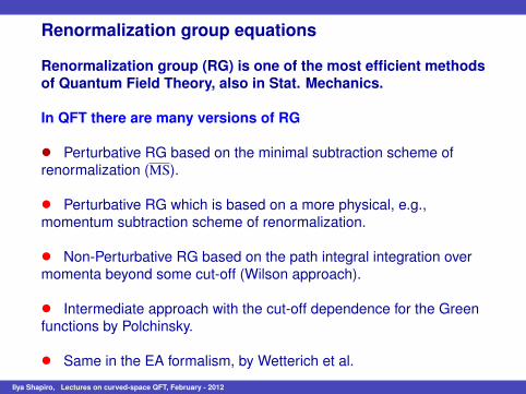
Renormalization group equations
Renormalization group (RG) is one of the most efficient methods of Quantum Field Theory, also in Stat. Mechanics.
In QFT there are many versions of RG
• Perturbative RG based on the minimal subtraction scheme of renormalization (MS).
• Perturbative RG which is based on a more physical, e.g., momentum subtraction scheme of renormalization.
• Non-Perturbative RG based on the path integral integration over momenta beyond some cut-off (Wilson approach).
• Intermediate approach with the cut-off dependence for the Green functions by Polchinsky.
• Same in the EA formalism, by Wetterich et al.
Ilya Shapiro, Lectures on curved-space QFT, February - 2012
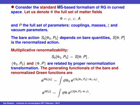
• Consider the standard MS-based formalism of RG in curved space. Let us denote Φ the full set of matter fields
Φ = φ, ψ, A
and P the full set of parameters: couplings, masses, ξ and vacuum parameters.
The bare action S0[Φ0,P0] depends on bare quantities, S[Φ,P] is the renormalized action.
Multiplicative renormalizability:
(Φ0,P0) and (Φ,P) are related by proper renormalization transformation. The generating functionals of the bare and renormalized Green functions are
eiW0[J0] =
eiW [J] =
Ilya Shapiro, Lectures on curved-space QFT, February - 2012
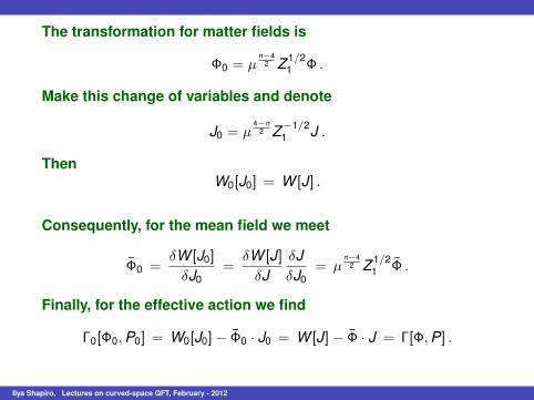
The transformation for matter fields is
Φ0 = µ n−4
Make this change of variables and denote
J0 = µ 4−n
Consequently, for the mean field we meet
Φ0 = δW [J0]
Finally, for the effective action we find
Γ0[Φ0,P0] = W0[J0]− Φ0 · J0 = W [J]− Φ · J = Γ[Φ,P] .
Ilya Shapiro, Lectures on curved-space QFT, February - 2012
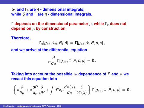
S0 and Γ0 are 4 - dimensional integrals, while S and Γ are n - dimensional integrals.
Γ depends on the dimensional parameter µ, while Γ0 does not depend on µ by construction.
Therefore, Γ0[gαβ ,Φ0,P0,4] = Γ[gαβ ,Φ,P, n, µ] ,
and we arrive at the differential equation
µ d
dµ Γ[gαβ ,Φ,P, n, µ] = 0 .
Taking into account the possible µ- dependence of P and Φ we recast this equation into{
µ ∂
Ilya Shapiro, Lectures on curved-space QFT, February - 2012
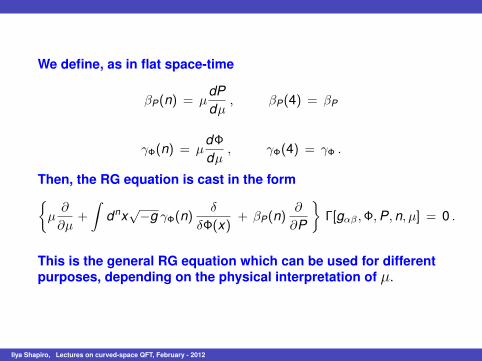
We define, as in flat space-time
βP(n) = µ dP dµ
Then, the RG equation is cast in the form{ µ ∂
∂µ +
∫ dnx
} Γ[gαβ ,Φ,P, n, µ] = 0 .
This is the general RG equation which can be used for different purposes, depending on the physical interpretation of µ.
Ilya Shapiro, Lectures on curved-space QFT, February - 2012
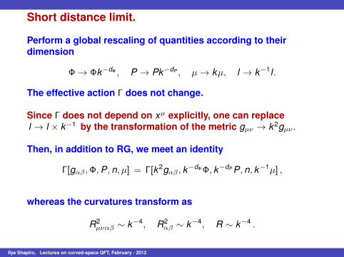
Short distance limit.
Perform a global rescaling of quantities according to their dimension
Φ → Φk−dΦ , P → Pk−dP , µ→ kµ, l → k−1l .
The effective action Γ does not change.
Since Γ does not depend on xµ explicitly, one can replace l → l × k−1 by the transformation of the metric gµν → k2gµν .
Then, in addition to RG, we meet an identity
Γ[gαβ ,Φ,P, n, µ] = Γ[k2gαβ , k−dΦΦ, k−dP P,n, k−1µ] ,
whereas the curvatures transform as
R2 µναβ ∼ k−4, R2
αβ ∼ k−4, R ∼ k−4 .
Ilya Shapiro, Lectures on curved-space QFT, February - 2012
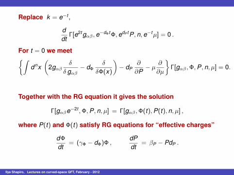
Replace k = e−t ,
For t = 0 we meet{∫ dnx
( 2gαβ
δ
Together with the RG equation it gives the solution
Γ[gαβe−2t ,Φ,P, n, µ] = Γ[gαβ ,Φ(t),P(t),n, µ] ,
where P(t) and Φ(t) satisfy RG equations for “effective charges”
dΦ dt
Ilya Shapiro, Lectures on curved-space QFT, February - 2012
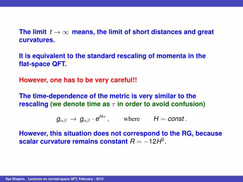
The limit t → ∞ means, the limit of short distances and great curvatures.
It is equivalent to the standard rescaling of momenta in the flat-space QFT.
However, one has to be very careful!!
The time-dependence of the metric is very similar to the rescaling (we denote time as τ in order to avoid confusion)
gαβ → gαβ · eHτ , where H = const .
However, this situation does not correspond to the RG, because scalar curvature remains constant R = −12H2.
Ilya Shapiro, Lectures on curved-space QFT, February - 2012
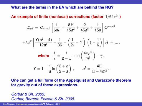
What are the terms in the EA which are behind the RG?
An example of finite (nonlocal) corrections (factor 1/64π2 ,)
Leff = Cµναβ
36 −
4 − 4m2 .
One can get a full form of the Appelquist and Carazzone theorem for gravity out of these expressions.
Gorbar & Sh. 2003; Gorbar, Berredo-Peixoto & Sh. 2005.
Ilya Shapiro, Lectures on curved-space QFT, February - 2012
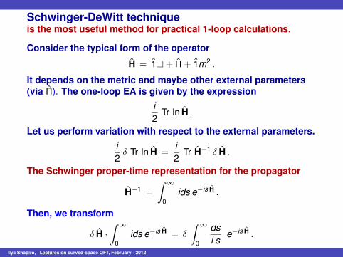
Schwinger-DeWitt technique is the most useful method for practical 1-loop calculations.
Consider the typical form of the operator
H = 1+ Π + 1m2 .
It depends on the metric and maybe other external parameters (via Π). The one-loop EA is given by the expression
i 2
Tr ln H .
Let us perform variation with respect to the external parameters. i 2 δ Tr ln H =
i 2
The Schwinger proper-time representation for the propagator
H−1 =
Then, we transform
∫ ∞
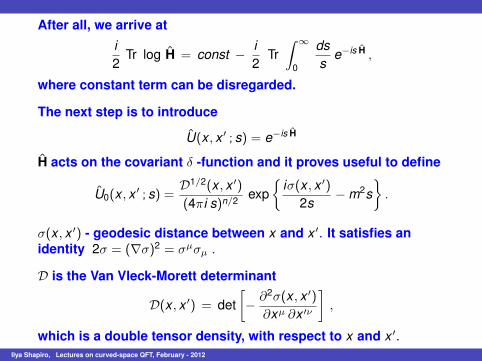
After all, we arrive at i 2
Tr log H = const − i 2
Tr ∫ ∞
0
where constant term can be disregarded.
The next step is to introduce
U(x , x ′ ; s) = e−is H
H acts on the covariant δ -function and it proves useful to define
U0(x , x ′ ; s) = D1/2(x , x ′)
(4πi s)n/2 exp {
} .
σ(x , x ′) - geodesic distance between x and x ′. It satisfies an identity 2σ = (∇σ)2 = σµσµ .
D is the Van Vleck-Morett determinant
D(x , x ′) = det [ − ∂2σ(x , x ′)
∂xµ ∂x ′ν
] ,
which is a double tensor density, with respect to x and x ′. Ilya Shapiro, Lectures on curved-space QFT, February - 2012
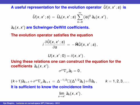
A useful representation for the evolution operator U(x , x ′ ; s) is
U(x , x ′ ; s) = U0(x , x ′ ; s) ∞∑
k=0
i ∂U(x , x ′ ; s)
∂s = − HU(x , x ′ ; s) ,
U(x , x ′ ; 0) = δ(x , x ′) .
Using these relations one can construct the equation for the coefficients ak (x , x ′).
σµ∇µa0 = 0 ,
(k+1)ak+1+σ µ∇µak+1 = −1/2(1/2ak )+Πak , k = 1,2, 3, ... .
It is sufficient to know the coincidence limits
lim x→x′
ak (x , x ′) .
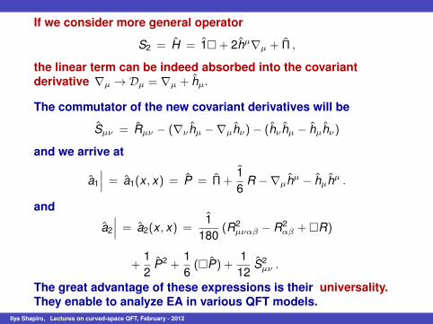
If we consider more general operator
S2 = H = 1+ 2hµ∇µ + Π ,
the linear term can be indeed absorbed into the covariant derivative ∇µ → Dµ = ∇µ + hµ.
The commutator of the new covariant derivatives will be
Sµν = Rµν − (∇ν hµ −∇µhν)− (hν hµ − hµhν)
and we arrive at
R −∇µhµ − hµhµ .
1 12
S2 µν .
The great advantage of these expressions is their universality. They enable to analyze EA in various QFT models.
Ilya Shapiro, Lectures on curved-space QFT, February - 2012
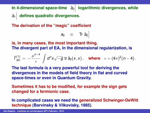
In 4-dimensional space-time a2
a2 ≡ Tr a2
is, in many cases, the most important thing. The divergent part of EA, in the dimensional regularization, is
Γ (1) div = − µn−4

∫ dnx
√ −g tr a2(x , x) , where = (4π)2(n − 4) .
The last formula is a very powerful tool for deriving the divergences in the models of field theory in flat and curved space-times or even in Quantum Gravity.
Sometimes it has to be modified, for example the sign gets changed for a fermionic case.
In complicated cases we need the generalized Schwinger-DeWitt technique (Barvinsky & Vilkovisky, 1985).
Ilya Shapiro, Lectures on curved-space QFT, February - 2012
Further coefficients ak , k ≥ 3 correspond to the finite part.
They are given by the expressions like
1 m2 O(R3) ,
and therefore contribute only to the finite part of EA.
Practical calculation of the coefficients ak , k ≥ 3 is possible, despite rather difficult.
The a3 coefficient has been derived by Gilkey (1979) and by Avramidy (1986), who also derived a4 coefficient. In 1989-1990 I. Avramidy and A. Barvinsky & G.V. Vilkovisky derived important resummation of the Schwinger-DeWitt series. As an important application one can obtain, for massive theories, the exact one-loop form factors of the terms
R2 , C2 , F 2 µν , (∇)2 , 4 .
E.Gorbar, I.Sh., G.de Berredo-Peixoto, B.Gonçalves, JHEP (2003); CQG (2005); PRD (2009).
Ilya Shapiro, Lectures on curved-space QFT, February - 2012
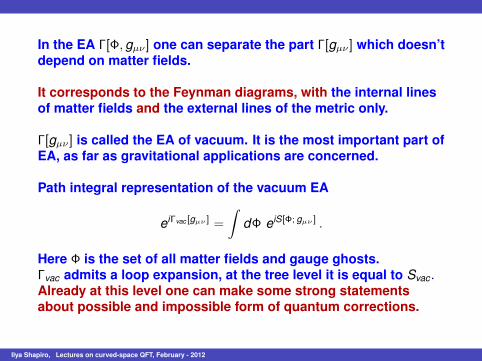
In the EA Γ[Φ, gµν ] one can separate the part Γ[gµν ] which doesn’t depend on matter fields.
It corresponds to the Feynman diagrams, with the internal lines of matter fields and the external lines of the metric only.
Γ[gµν ] is called the EA of vacuum. It is the most important part of EA, as far as gravitational applications are concerned.
Path integral representation of the vacuum EA
eiΓvac [gµν ] =
∫ dΦ eiS[Φ; gµν ] .
Here Φ is the set of all matter fields and gauge ghosts. Γvac admits a loop expansion, at the tree level it is equal to Svac . Already at this level one can make some strong statements about possible and impossible form of quantum corrections.
Ilya Shapiro, Lectures on curved-space QFT, February - 2012
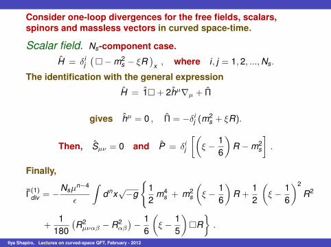
Consider one-loop divergences for the free fields, scalars, spinors and massless vectors in curved space-time.
Scalar field. Ns-component case.
H = δi j ( − m2
The identification with the general expression
H = 1+ 2hµ∇µ + Π
gives hµ = 0 , Π = −δi j (m
2 s + ξR).
[( ξ − 1
Ilya Shapiro, Lectures on curved-space QFT, February - 2012
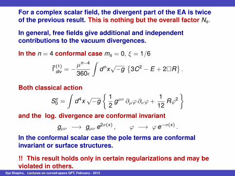
For a complex scalar field, the divergent part of the EA is twice of the previous result. This is nothing but the overall factor Ns.
In general, free fields give additional and independent contributions to the vacuum divergences.
In the n = 4 conformal case ms = 0, ξ = 1/6
Γ (1) div = −µ
} and the log. divergence are conformal invariant
gµν −→ gµν e2σ(x) , φ −→ φ e−σ(x) .
In the conformal scalar case the pole terms are conformal invariant or surface structures.
!! This result holds only in certain regularizations and may be violated in others.
Ilya Shapiro, Lectures on curved-space QFT, February - 2012
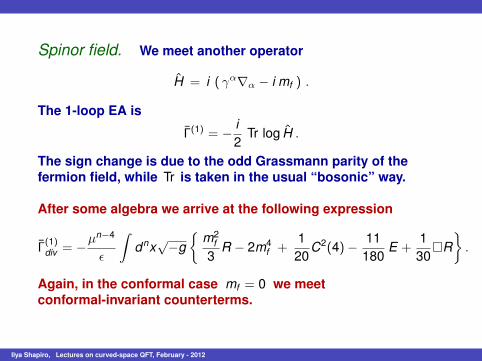
Spinor field. We meet another operator
H = i ( γα∇α − i mf ) .
The 1-loop EA is
Γ(1) = − i 2
Tr log H .
The sign change is due to the odd Grassmann parity of the fermion field, while Tr is taken in the usual “bosonic” way.
After some algebra we arrive at the following expression
Γ (1) div = −µ
} .
Again, in the conformal case mf = 0 we meet conformal-invariant counterterms.
Ilya Shapiro, Lectures on curved-space QFT, February - 2012
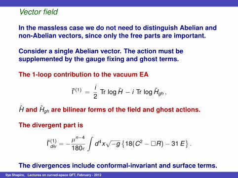
Vector field
In the massless case we do not need to distinguish Abelian and non-Abelian vectors, since only the free parts are important.
Consider a single Abelian vector. The action must be supplemented by the gauge fixing and ghost terms.
The 1-loop contribution to the vacuum EA
Γ(1) = i 2
Tr log H − i Tr log Hgh ,
H and Hgh are bilinear forms of the field and ghost actions.
The divergent part is
Γ (1) div = −µ
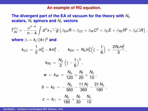
An example of RG equation.
The divergent part of the EA of vacuum for the theory with Ns scalars, Nf spinors and Nv vectors
Γ (1) div = − µn−4
n − 4
} ,
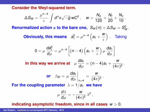
Consider the Weyl-squared term.
Ns
120 +
Nf
20 +
Nv
10 .
Renormalized action = to the bare one, SW (n) + SW = S0 W .
Obviously, this means a0 1 = µn−4
( a1 +
da1
µ dλ dµ
= − w (4π)2 λ
2 ,
indicating asymptotic freedom, since in all cases w > 0. Ilya Shapiro, Lectures on curved-space QFT, February - 2012
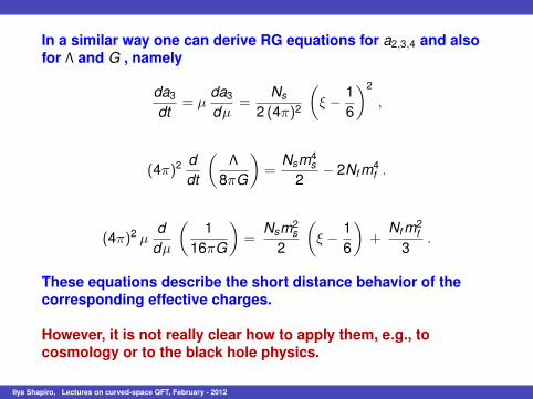
In a similar way one can derive RG equations for a2,3,4 and also for Λ and G , namely
da3
These equations describe the short distance behavior of the corresponding effective charges.
However, it is not really clear how to apply them, e.g., to cosmology or to the black hole physics.
Ilya Shapiro, Lectures on curved-space QFT, February - 2012
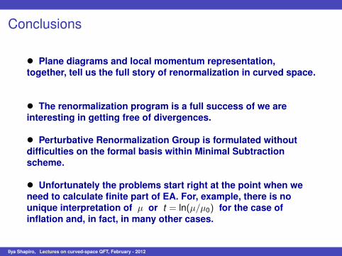
Conclusions
• Plane diagrams and local momentum representation, together, tell us the full story of renormalization in curved space.
• The renormalization program is a full success of we are interesting in getting free of divergences.
• Perturbative Renormalization Group is formulated without difficulties on the formal basis within Minimal Subtraction scheme.
• Unfortunately the problems start right at the point when we need to calculate finite part of EA. For, example, there is no unique interpretation of µ or t = ln(µ/µ0) for the case of inflation and, in fact, in many other cases.
Ilya Shapiro, Lectures on curved-space QFT, February - 2012