Wilson loops at strong coupling for curved...
23
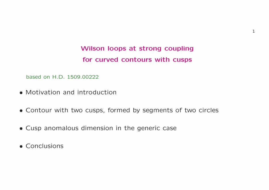
1 Wilson loops at strong coupling for curved contours with cusps based on H.D. 1509.00222 • Motivation and introduction • Contour with two cusps, formed by segments of two circles • Cusp anomalous dimension in the generic case • Conclusions
Transcript of Wilson loops at strong coupling for curved...
1
Wilson loops at strong coupling
for curved contours with cusps
based on H.D. 1509.00222
• Motivation and introduction
• Contour with two cusps, formed by segments of two circles
• Cusp anomalous dimension in the generic case
• Conclusions
2Introduction
Local supersymmetric Wilson (Maldacena) loop in N = 4 SYM
W [C] = 1N 〈trP exp
∫
C i(Aµ(x(τ))xµ + ΦIθI(x)|x|)dτ〉
C : xµ(τ) closed path in R1,3, θI(x) closed path in S5.
In non-SUSY gauge theories like QCD blue terms absent.
UV properties for smooth contours C:
N = 4 SYM: finite, invariance under conformal maps of C
QCD: No further renormalisation, beyond that necessary for local
correlation functions Polyakov 1979, Dotsenko, Vergeles 1980 ...
Note: Everything disregarding a linear divergence proportional to the length of C.
(It is anyway absent in the SUSY case. Drukker, Gross, Ooguri 1999)
3Introduction
UV properties for contours with cusps: Both in N = 4 SYM and QCD
renormalisation requires cusp anomalous dimension Γ(g, θ), depending on
the coupling and the angle
QCD: one loop Polyakov 1980, two loops Korchemsky, Radyushkin 1987,
three loops Grozin, Henn, Korchemsky, Marquard 2014
N = 4 SYM: ..., four loops (planar limit) Henn, Huber 2013
Strong coupling, input from AdS/CFT:
W [C] in N = 4 SYM ⇐⇒ string partition fct. in AdS5 × S5 with b. c.:
string surface appr. contour C on conformal boundary of AdS5 × S5
Maldacena; Rey/Yee 1998
For λ = g2N → ∞ : logW = −√λ
2πA + O(logλ) , A area
4Introduction
The construction uses Poincare coordinates (conf. bound. at r = 0)
ds2 =1
r2
(
dxµdxµ + dr2)
.
UV divergences ⇐⇒ div. of area due to blow up of metric near r = 0.
Regularised area Aǫ: cut off parts of surface with r < ǫ.
Surfaces for smooth contours near boundary Graham, Witten 1999;
Polyakov, Rychkov 2000
xµ(σ, r) = xµ(σ,0) +1
2
d2
dσ2xµ(σ,0) r2 + O(r3) .
Crucial: no terms linear in r !!
This implies for smooth contours
Aǫ =l
ǫ+ Aren + O(ǫ) .
5Introduction
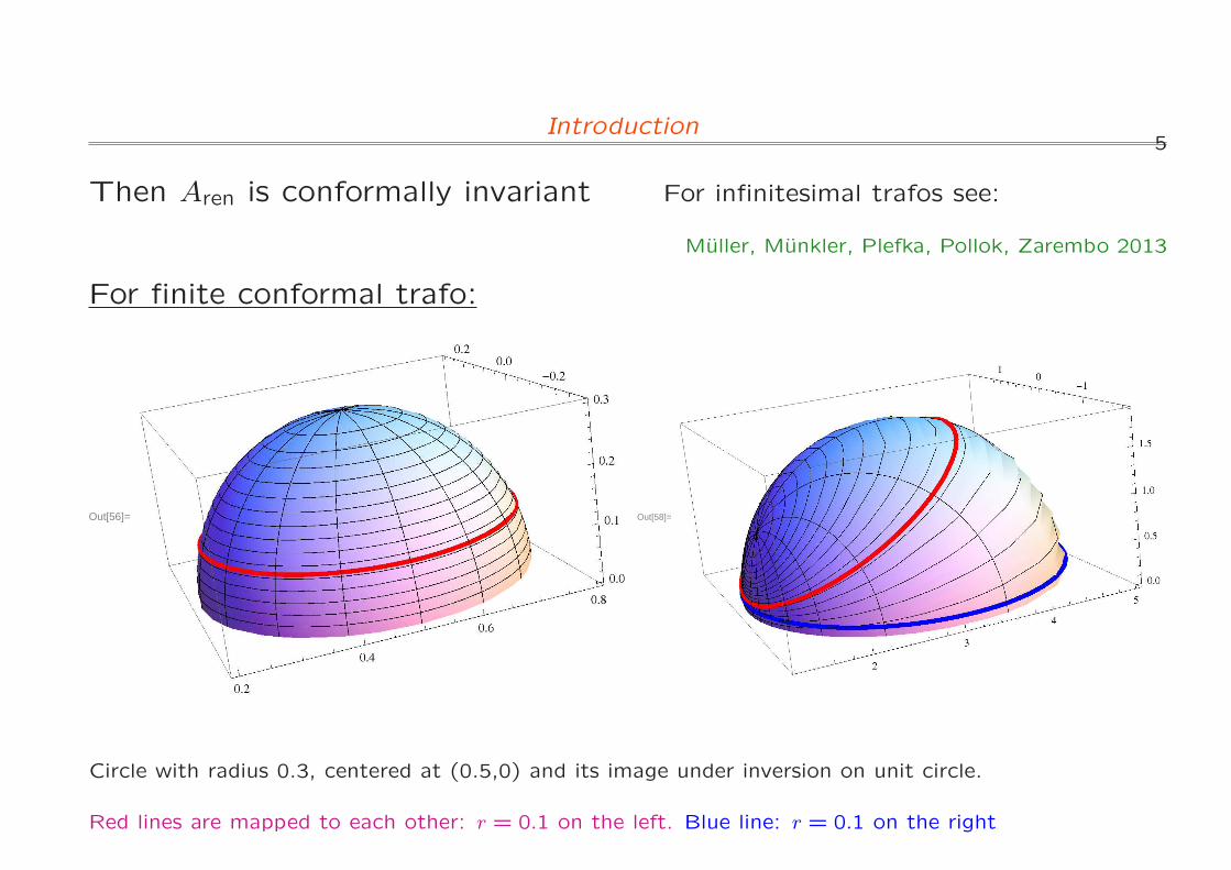
Then Aren is conformally invariant For infinitesimal trafos see:
Muller, Munkler, Plefka, Pollok, Zarembo 2013
For finite conformal trafo:
Out[56]= Out[58]=
Circle with radius 0.3, centered at (0.5,0) and its image under inversion on unit circle.
Red lines are mapped to each other: r = 0.1 on the left. Blue line: r = 0.1 on the right
6Introduction
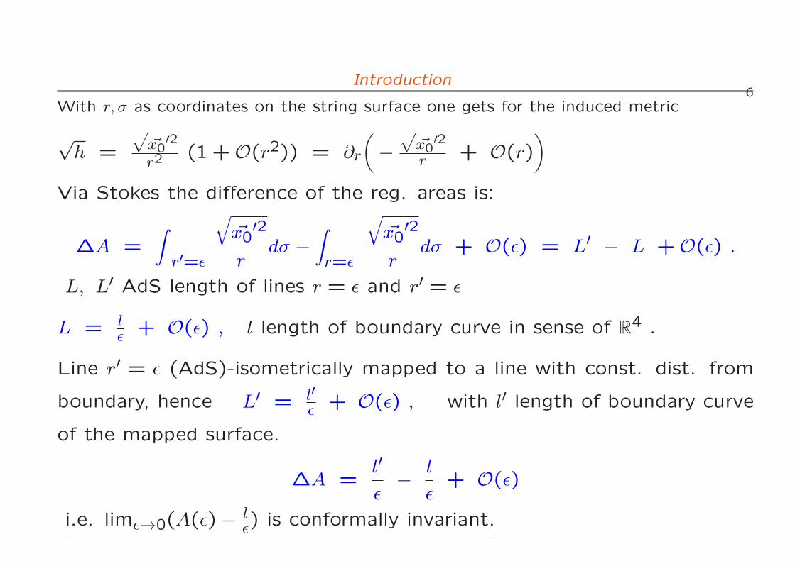
With r, σ as coordinates on the string surface one gets for the induced metric
√h =
√
~x0′2
r2(1 +O(r2)) = ∂r
(
−√
~x0′2
r + O(r)
)
Via Stokes the difference of the reg. areas is:
∆A =∫
r′=ǫ
√
~x0′2
rdσ −
∫
r=ǫ
√
~x0′2
rdσ + O(ǫ) = L′ − L +O(ǫ) .
L, L′ AdS length of lines r = ǫ and r′ = ǫ
L = lǫ + O(ǫ) , l length of boundary curve in sense of R
4 .
Line r′ = ǫ (AdS)-isometrically mapped to a line with const. dist. from
boundary, hence L′ = l′ǫ + O(ǫ) , with l′ length of boundary curve
of the mapped surface.
∆A =l′
ǫ− l
ǫ+ O(ǫ)
i.e. limǫ→0(A(ǫ)− lǫ) is conformally invariant.
7Introduction and Motivation
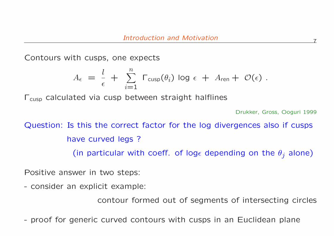
Contours with cusps, one expects
Aǫ =l
ǫ+
n∑
i=1
Γcusp(θi) log ǫ + Aren + O(ǫ) .
Γcusp calculated via cusp between straight halflines
Drukker, Gross, Ooguri 1999
Question: Is this the correct factor for the log divergences also if cusps
have curved legs ?
(in particular with coeff. of logǫ depending on the θj alone)
Positive answer in two steps:
- consider an explicit example:
contour formed out of segments of intersecting circles
- proof for generic curved contours with cusps in an Euclidean plane
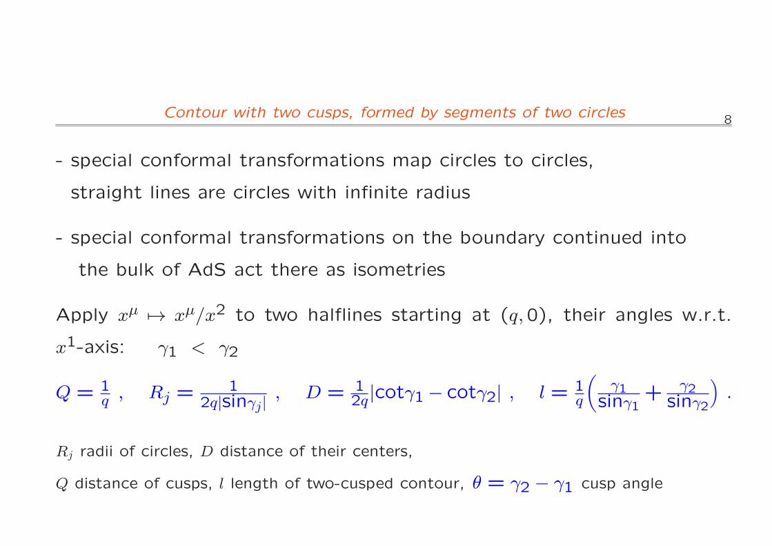
8Contour with two cusps, formed by segments of two circles
- special conformal transformations map circles to circles,
straight lines are circles with infinite radius
- special conformal transformations on the boundary continued into
the bulk of AdS act there as isometries
Apply xµ 7→ xµ/x2 to two halflines starting at (q,0), their angles w.r.t.
x1-axis: γ1 < γ2
Q = 1q , Rj =
12q|sinγj|
, D = 12q |cotγ1− cotγ2| , l = 1
q
(
γ1sinγ1
+ γ2sinγ2
)
.
Rj radii of circles, D distance of their centers,
Q distance of cusps, l length of two-cusped contour, θ = γ2 − γ1 cusp angle
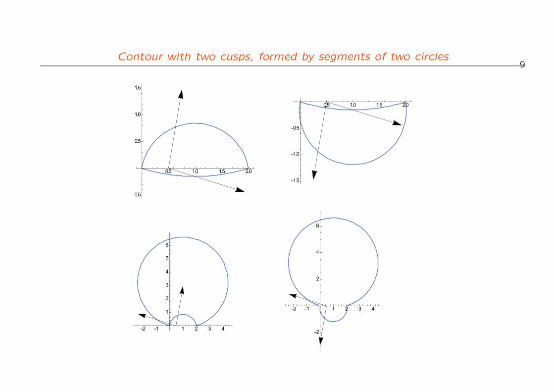
9Contour with two cusps, formed by segments of two circles
10Contour with two cusps, formed by segments of two circles
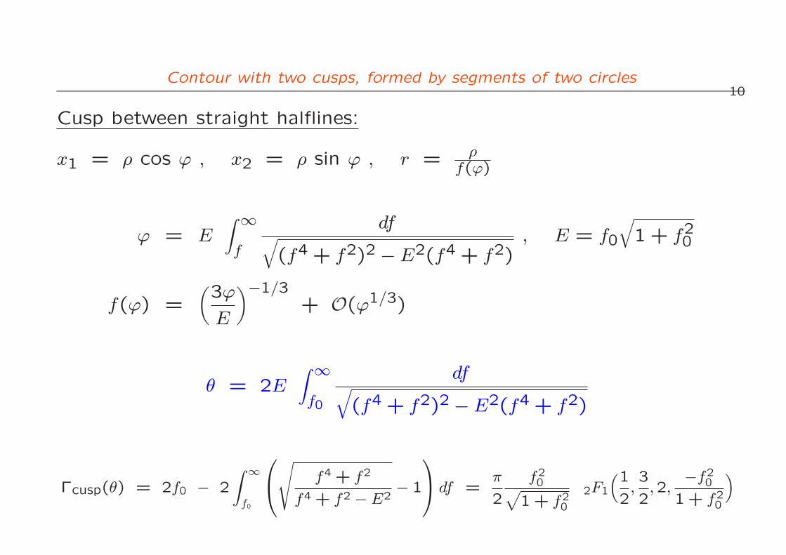
Cusp between straight halflines:
x1 = ρ cos ϕ , x2 = ρ sin ϕ , r = ρf(ϕ)
ϕ = E∫ ∞
f
df√
(f4 + f2)2 − E2(f4 + f2), E = f0
√
1+ f20
f(ϕ) =
(
3ϕ
E
)−1/3+ O(ϕ1/3)
θ = 2E∫ ∞
f0
df√
(f4 + f2)2 − E2(f4 + f2)
Γcusp(θ) = 2f0 − 2
∫ ∞
f0
√
f4 + f2
f4 + f2 − E2− 1
df =π
2
f20
√
1+ f20
2F1
(1
2,3
2,2,
−f20
1+ f20
)
11Contour with two cusps, formed by segments of two circles
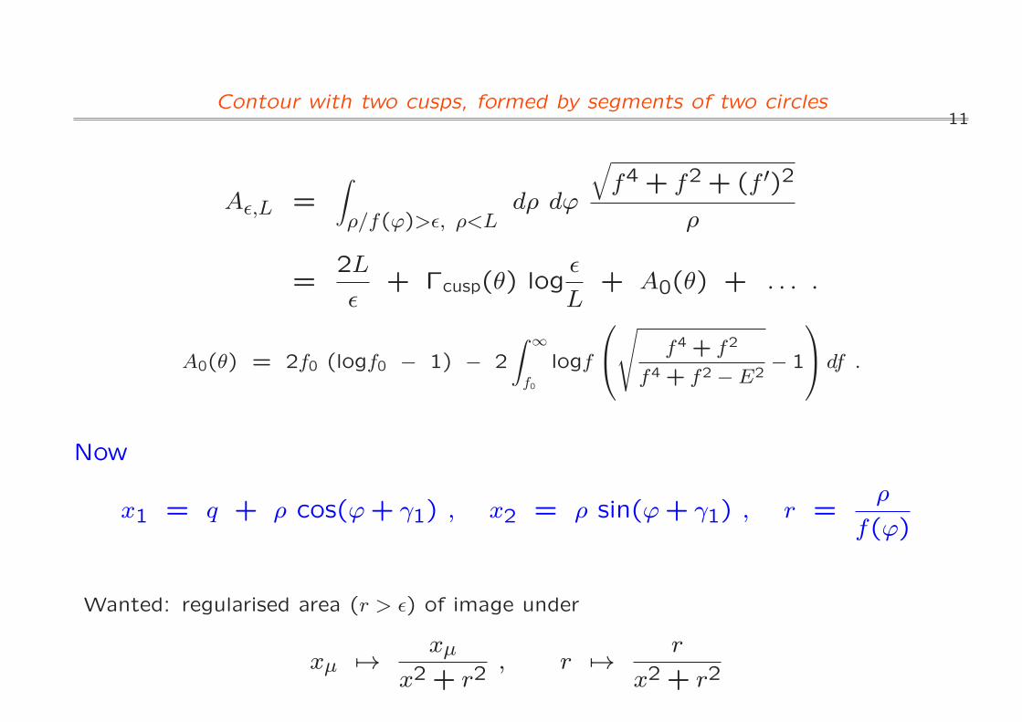
Aǫ,L =∫
ρ/f(ϕ)>ǫ, ρ<Ldρ dϕ
√
f4 + f2 + (f ′)2
ρ
=2L
ǫ+ Γcusp(θ) log
ǫ
L+ A0(θ) + . . . .
A0(θ) = 2f0 (logf0 − 1) − 2
∫ ∞
f0
logf
√
f4 + f2
f4 + f2 − E2− 1
df .
Now
x1 = q + ρ cos(ϕ+ γ1) , x2 = ρ sin(ϕ+ γ1) , r =ρ
f(ϕ)
Wanted: regularised area (r > ǫ) of image under
xµ 7→ xµ
x2 + r2, r 7→ r
x2 + r2
12Contour with two cusps, formed by segments of two circles
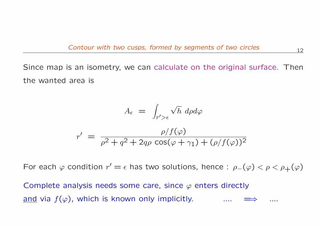
Since map is an isometry, we can calculate on the original surface. Then
the wanted area is
Aǫ =∫
r′>ǫ
√h dρdϕ
r′ =ρ/f(ϕ)
ρ2 + q2 +2qρ cos(ϕ+ γ1) + (ρ/f(ϕ))2
For each ϕ condition r′ = ǫ has two solutions, hence : ρ−(ϕ) < ρ < ρ+(ϕ)
Complete analysis needs some care, since ϕ enters directly
and via f(ϕ), which is known only implicitly. .... =⇒ ....
13Contour with two cusps, formed by segments of two circles
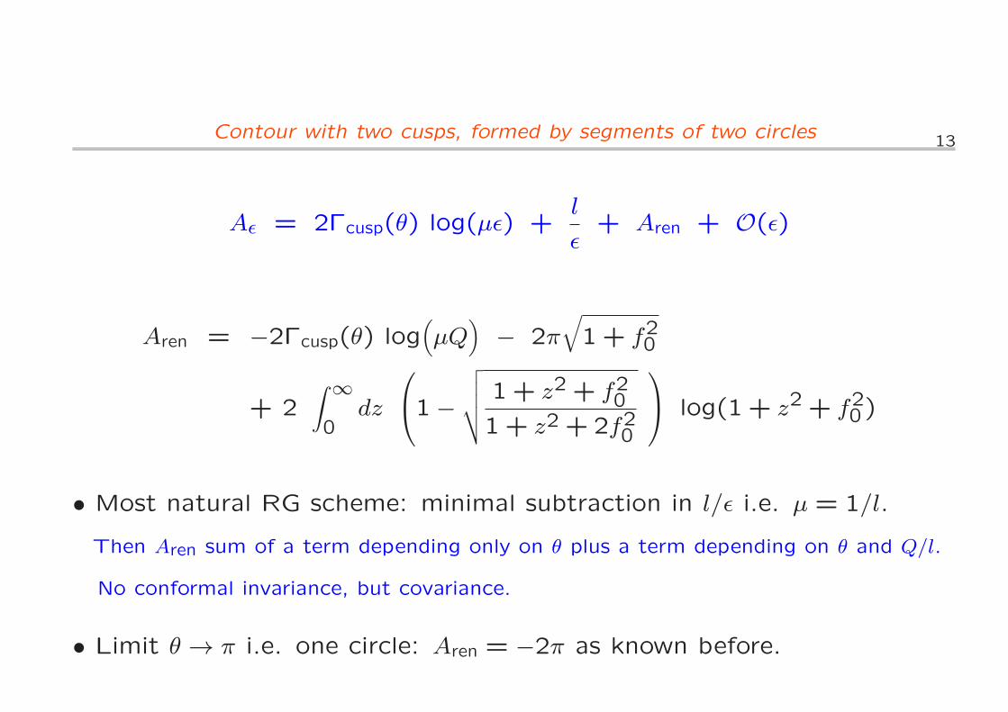
Aǫ = 2Γcusp(θ) log(µǫ) +l
ǫ+ Aren + O(ǫ)
Aren = −2Γcusp(θ) log(
µQ)
− 2π√
1+ f20
+ 2∫ ∞
0dz
1−√
√
√
√
1+ z2 + f201+ z2 +2f20
log(1 + z2 + f20)
• Most natural RG scheme: minimal subtraction in l/ǫ i.e. µ = 1/l.
Then Aren sum of a term depending only on θ plus a term depending on θ and Q/l.
No conformal invariance, but covariance.
• Limit θ → π i.e. one circle: Aren = −2π as known before.
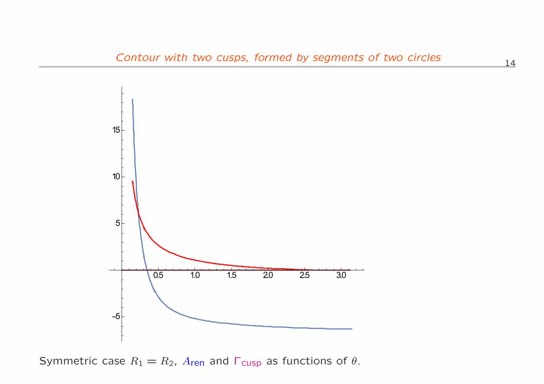
14Contour with two cusps, formed by segments of two circles
Symmetric case R1 = R2, Aren and Γcusp as functions of θ.
15Cusp anomalous dimension in the generic case
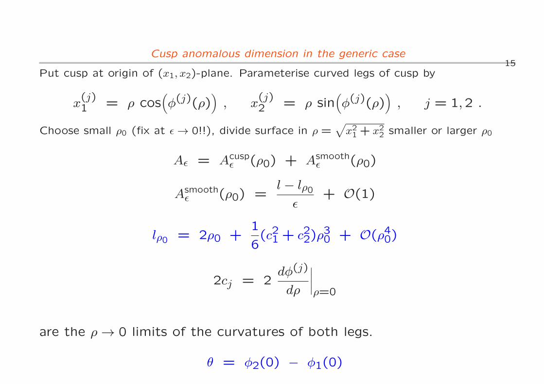
Put cusp at origin of (x1, x2)-plane. Parameterise curved legs of cusp by
x(j)1 = ρ cos
(
φ(j)(ρ))
, x(j)2 = ρ sin
(
φ(j)(ρ))
, j = 1,2 .
Choose small ρ0 (fix at ǫ → 0!!), divide surface in ρ =√
x21 + x2
2 smaller or larger ρ0
Aǫ = Acuspǫ (ρ0) + Asmooth
ǫ (ρ0)
Asmoothǫ (ρ0) =
l − lρ0ǫ
+ O(1)
lρ0 = 2ρ0 +1
6(c21 + c22)ρ
30 + O(ρ40)
2cj = 2dφ(j)
dρ
∣
∣
∣
∣
ρ=0
are the ρ → 0 limits of the curvatures of both legs.
θ = φ2(0) − φ1(0)
16Cusp anomalous dimension in the generic case
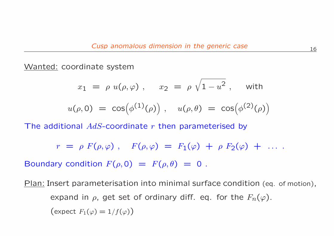
Wanted: coordinate system
x1 = ρ u(ρ, ϕ) , x2 = ρ
√
1− u2 , with
u(ρ,0) = cos(
φ(1)(ρ))
, u(ρ, θ) = cos(
φ(2)(ρ))
The additional AdS-coordinate r then parameterised by
r = ρ F (ρ, ϕ) , F (ρ, ϕ) = F1(ϕ) + ρ F2(ϕ) + . . . .
Boundary condition F (ρ,0) = F (ρ, θ) = 0 .
Plan: Insert parameterisation into minimal surface condition (eq. of motion),
expand in ρ, get set of ordinary diff. eq. for the Fn(ϕ).
(expect F1(ϕ) = 1/f(ϕ))
17Cusp anomalous dimension in the generic case
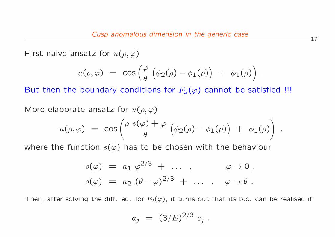
First naive ansatz for u(ρ, ϕ)
u(ρ, ϕ) = cos
(
ϕ
θ
(
φ2(ρ)− φ1(ρ))
+ φ1(ρ)
)
.
But then the boundary conditions for F2(ϕ) cannot be satisfied !!!
More elaborate ansatz for u(ρ, ϕ)
u(ρ, ϕ) = cos
(
ρ s(ϕ) + ϕ
θ
(
φ2(ρ)− φ1(ρ))
+ φ1(ρ)
)
,
where the function s(ϕ) has to be chosen with the behaviour
s(ϕ) = a1 ϕ2/3 + . . . , ϕ → 0 ,
s(ϕ) = a2 (θ − ϕ)2/3 + . . . , ϕ → θ .
Then, after solving the diff. eq. for F2(ϕ), it turns out that its b.c. can be realised if
aj = (3/E)2/3 cj .
18Cusp anomalous dimension in the generic case
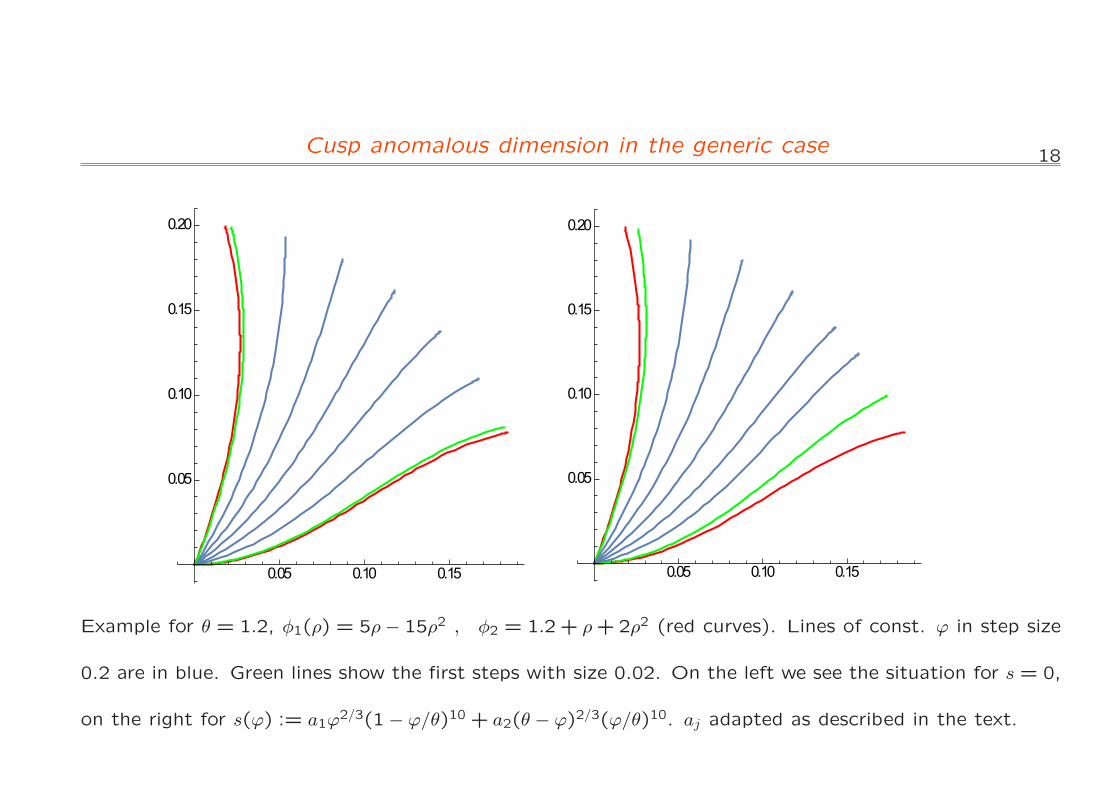
Example for θ = 1.2, φ1(ρ) = 5ρ− 15ρ2 , φ2 = 1.2+ ρ+2ρ2 (red curves). Lines of const. ϕ in step size
0.2 are in blue. Green lines show the first steps with size 0.02. On the left we see the situation for s = 0,
on the right for s(ϕ) := a1ϕ2/3(1− ϕ/θ)10 + a2(θ − ϕ)2/3(ϕ/θ)10. aj adapted as described in the text.
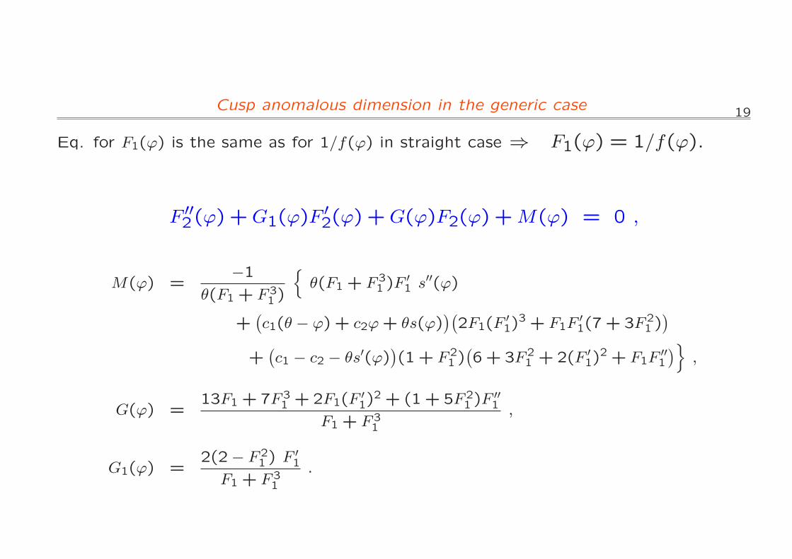
19Cusp anomalous dimension in the generic case
Eq. for F1(ϕ) is the same as for 1/f(ϕ) in straight case ⇒ F1(ϕ) = 1/f(ϕ).
F ′′2(ϕ) +G1(ϕ)F
′2(ϕ) +G(ϕ)F2(ϕ) +M(ϕ) = 0 ,
M(ϕ) =−1
θ(F1 + F 31 )
{
θ(F1 + F 31 )F
′1 s′′(ϕ)
+(
c1(θ − ϕ) + c2ϕ+ θs(ϕ))(
2F1(F′1)
3 + F1F′1(7 + 3F 2
1 ))
+(
c1 − c2 − θs′(ϕ))
(1 + F 21 )(
6+ 3F 21 +2(F ′
1)2 + F1F
′′1
)
}
,
G(ϕ) =13F1 +7F 3
1 +2F1(F ′1)
2 + (1+ 5F 21 )F
′′1
F1 + F 31
,
G1(ϕ) =2(2− F 2
1 ) F ′1
F1 + F 31
.
20Cusp anomalous dimension in the generic case
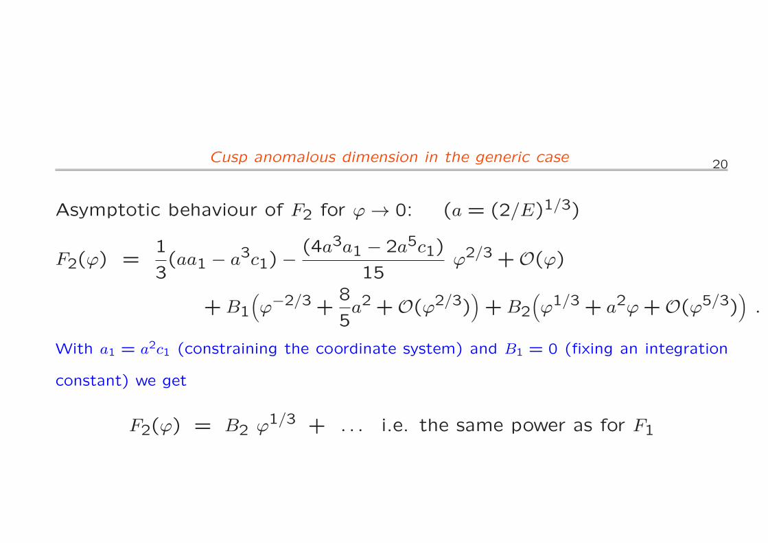
Asymptotic behaviour of F2 for ϕ → 0: (a = (2/E)1/3)
F2(ϕ) =1
3(aa1 − a3c1)−
(4a3a1 − 2a5c1)
15ϕ2/3 +O(ϕ)
+B1
(
ϕ−2/3 +8
5a2 +O(ϕ2/3)
)
+B2
(
ϕ1/3 + a2ϕ+O(ϕ5/3))
.
With a1 = a2c1 (constraining the coordinate system) and B1 = 0 (fixing an integration
constant) we get
F2(ϕ) = B2 ϕ1/3 + . . . i.e. the same power as for F1
21Cusp anomalous dimension in the generic case
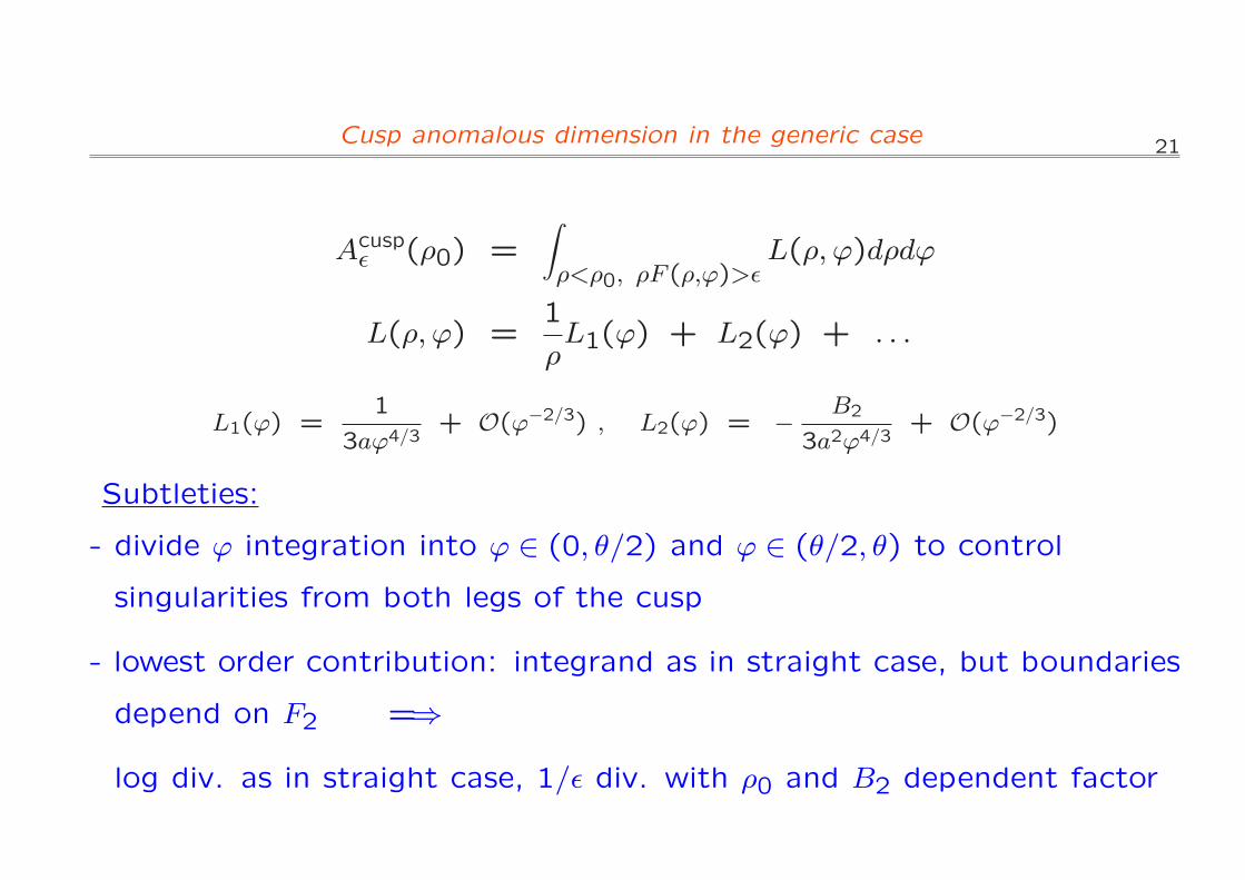
Acuspǫ (ρ0) =
∫
ρ<ρ0, ρF (ρ,ϕ)>ǫL(ρ, ϕ)dρdϕ
L(ρ, ϕ) =1
ρL1(ϕ) + L2(ϕ) + . . .
L1(ϕ) =1
3aϕ4/3+ O(ϕ−2/3) , L2(ϕ) = − B2
3a2ϕ4/3+ O(ϕ−2/3)
Subtleties:
- divide ϕ integration into ϕ ∈ (0, θ/2) and ϕ ∈ (θ/2, θ) to control
singularities from both legs of the cusp
- lowest order contribution: integrand as in straight case, but boundaries
depend on F2 =⇒
log div. as in straight case, 1/ǫ div. with ρ0 and B2 dependent factor
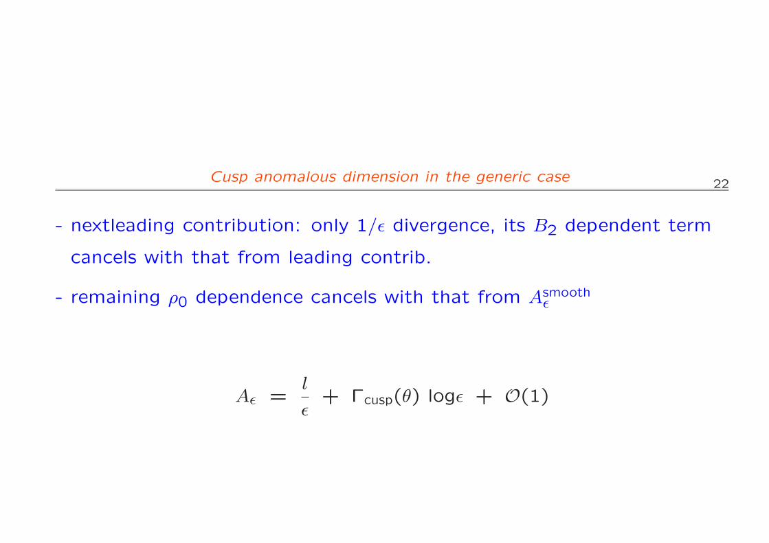
22Cusp anomalous dimension in the generic case
- nextleading contribution: only 1/ǫ divergence, its B2 dependent term
cancels with that from leading contrib.
- remaining ρ0 dependence cancels with that from Asmoothǫ
Aǫ =l
ǫ+ Γcusp(θ) logǫ + O(1)
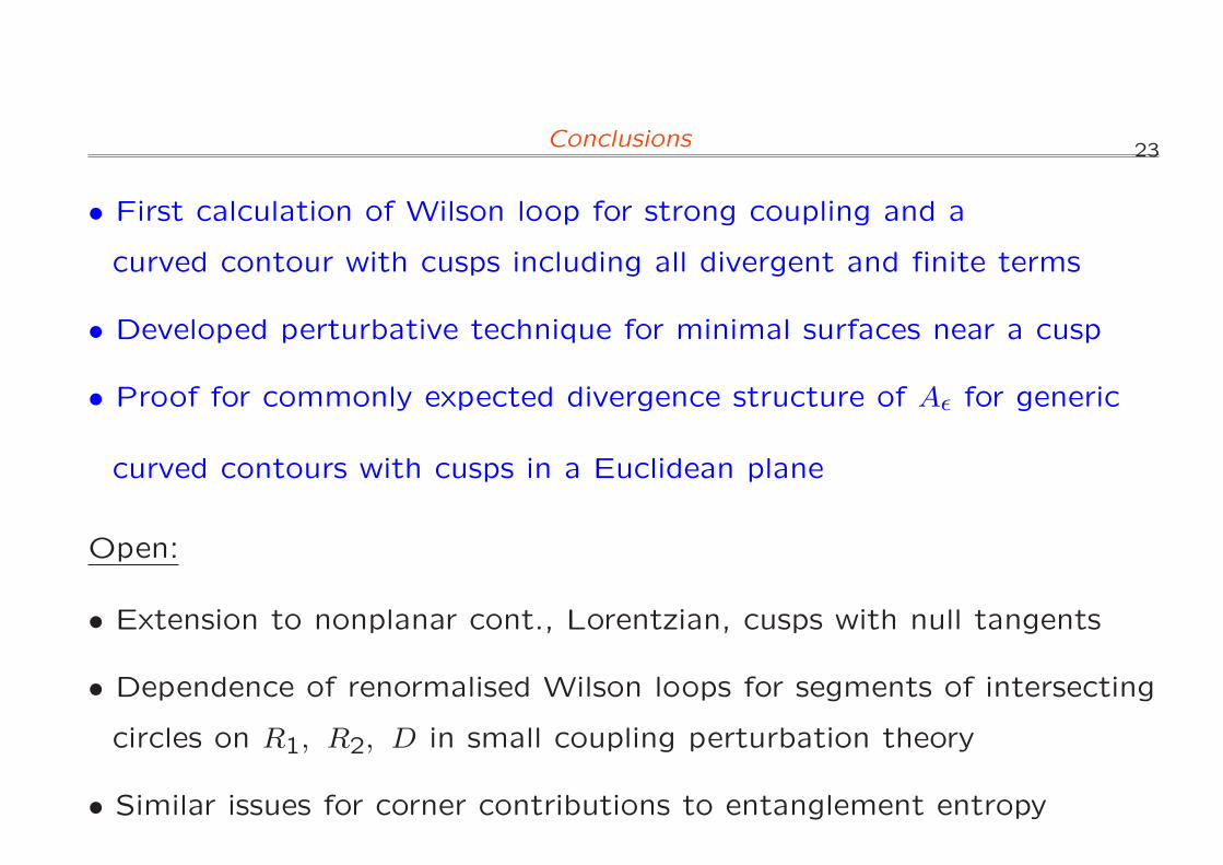
23Conclusions
• First calculation of Wilson loop for strong coupling and a
curved contour with cusps including all divergent and finite terms
• Developed perturbative technique for minimal surfaces near a cusp
• Proof for commonly expected divergence structure of Aǫ for generic
curved contours with cusps in a Euclidean plane
Open:
• Extension to nonplanar cont., Lorentzian, cusps with null tangents
• Dependence of renormalised Wilson loops for segments of intersecting
circles on R1, R2, D in small coupling perturbation theory
• Similar issues for corner contributions to entanglement entropy

![(Reference [2]) LINEAR PHASE LOCKED LOOPS - CONTINUED …pallen.ece.gatech.edu/Academic/ECE_6440/Summer_2003/L060-LPLL-II(2UP).pdf(Reference [2]) LINEAR PHASE LOCKED LOOPS - CONTINUED](https://static.fdocument.org/doc/165x107/6016ce84e4e4bb557426a4e4/reference-2-linear-phase-locked-loops-continued-2uppdf-reference-2-linear.jpg)


![The geodesic flow of a nonpositively curved graph manifold · 2018. 7. 24. · arXiv:math/9911170v1 [math.DG] 22 Nov 1999 The geodesic flow of a nonpositively curved graph manifold](https://static.fdocument.org/doc/165x107/5fdba015c36b0c2af5295c4f/the-geodesic-iow-of-a-nonpositively-curved-graph-manifold-2018-7-24-arxivmath9911170v1.jpg)