QFT in curved space-time

1 Introduction

1.1 The Einstein-Hilbert action (31.01.2010)

Before we turn to quantum field theory in curved space-times, we shortly review the classicaltheory of gravity. Einstein’s equations of classical general relativity can be derived from theEinstein-Hilbert action:

S =1

16πG

∫d4x√g(R− 2Λ).

with R the Ricci curvature and the cosmological constant Λ. Under a variation δgab, thevariation of the action is given by:

δS =1

16πG

∫d4x

(δ (√g) (R− 2Λ) +

√gδ (Rab) g

ab +√gRabδ

(gab)).

To analyze this expression, use:

δg = det (gab + δgab)− det gab = det gab

[det(gbc + δgbc

)− 1]

=

= det gab · Trδgbc = ggabδgab = −ggabδgab

gabδRab = gab (∂cδΓcab − ∂bδΓcac + ΓδΓ) = gab (∇cδΓcab −∇bδΓcac)

= ∇c(gabδΓcab − gabδΓcbc

)For the last derivation, we used normal coordinates around some point p, i.e. Γ|p = 0 to getrid of terms quadratic in the Christoffel symbols. Next, we replaced the partial derivatives bycovariant derivatives for the same reasons. Since the equation is now tensorial again, it holdseverywhere. In the last step, we used the property of the Levi-Cività connection, ∇agbc = 0.A slightly different derivation is given in [15], appendix E.The total derivative contributes only a boundary term, which can be eliminated adding anadditional piece 2

∫∂M K where K is the extrinsic curvature, K = hab∇anb, where hab =

gab±nanb is the induced metric on the boundary, and na is a normal vector on the boundary.Ignoring these subtleties (for example for a manifold without boundary), we get:

δS =1

16πG

∫d4x√g

(Rab −

1

2Rgab + Λgab

)δgab

resulting in Einstein’s equations in vacuum after setting the variation to zero.To add matter simply add another term to the action, p.e. a field strength term of Yang-Millsgauge theory or electromagnetism:

SM =

∫d4x√gLm =

1

4g2

∫TrF ∧ ?F =

1

4g2

∫d4x√gTrF abFab.

Define the energy-momentum tensor by Tab = 2√g

δ(√gLm)δgab

and get Einstein’s equations

Rab −1

2Rgab + Λgab = 8πGTab.

1

1.2 Attempts to quantize general relativity

General relativity is a classical field theory, with metric field gab, which plays a dual rôle,both being the dynamical variable in the game, and describing the background. Over the lastdecades there were various attempts to find a quantum theory of gravity. One of the majorlines are the following:

1. Covariant perturbation method: gab = g(0)ab +hab, where the first part solves the classical

Einstein equations. Write down Feynman rules. The problem of this attempt is thatthe perturbation theory is non-renormalizable. Let’s try to understand this.In natural units c = ~ = 1, the action is dimensionless. In dimension n, R has dimensionL−2, while the measure contributes Ln, so Newton’s constant GN has dimension Ln−2.In fact, GN = ln−2

p in these units, where lp is the n dimensional Planck length.So our coupling parameter is:

1

κ2=

1

16πGN=

1

16πln−2p

=Mn−2p

16π

with Planck mass Mp. So at a distance X-times smaller (or at momentum X-timeslarger), GN seems Xn−2-times larger, so GN ∼ pn−2 and the critical dimension is 2. Soin 4d, gravity seems non-renormalizable, i.e. gets stronger at shorter distances. In 4dimensions GN = l2p.Pure GR is finite to one-loop order (i.e. the divergences cancel due to an analogue ofthe Ward identity) but not in higher orders or if coupled to matter.Next step: supergravity. Make the theory supersymmetric, add a gravitino (spin 3/2),to cancel some divergences. Highest dimension (with one time dimension) is 11, so thisis the most natural setup. Get solutions in 4 dimensions by dimensional reduction (likein Kaluza-Klein theories).Finally: Perturbative String theory.

2. Canonical quantization method: Wheeler-DeWitt equation: H |Ψ〉 = 0. Backgroundindependance as a principle.This approach leads to Loop Quantum Gravity after introducing Ashtekar’s variables.

3. Path integral method: Try a generating functional:

Z =

∫D [gab] e−S

with the Einstein-Hilbert action S as above. It is not known how to define a measure onthe moduli space of metrics. Another problem is again non-renormalizability. In LQG,the moduli space is reduced, one ends up with the spin foam formulation.

4. Alternate routes: Twistor theory, gravitational OR (Roger Penrose), non-commutativegeometry (Alain Connes).

1.3 One step back: QFT in curved space-time

Lacking a full theory of gravity, let’s see how far we get without it. We saw above, that(reinserting ~) the Einstein Hilbert action in four dimensions is proportional to ~

l2p. Looking

2

at the formal path integral ∫D[gab] e−S =

∫D[gab] e

− ~l2p

∫R

it seems that quantum effects of gravity become important only at the order of the Plancklength. A first step towards quantum electrodynamics is to consider matter in a classicalbackground of an electromagnetic field. In analogy, we might hope to get some insight toquantum effects of gravity by considering quantized fields in a classical background, i.e. ina classical curved space. Still there are some issues with this idea. The principle of generalcovariance states that matter and mass couple equally strongly to gravity.Nevertheless, if we consider for example a free field theory, only one-loop 1PI diagrams arepossible (lacking interaction vertices). Up to order ~, we can therefore truncate gravity alsoto first-loop order.For an interacting theory of matter fields, higher loops of these fields are possible, so we shouldalso better include higher graviton loops. Recall the very different nature of the couplingconstant in, say, electromagnetism, and in Einstein gravity. In the first case, it is given by thedimensionless fine-structure constant α ' 1

137 , while for gravity, the coupling is dimension-full, being proportional to the Planck length. While one single graviton loop is of zeroth orderin GN , higher loops come from graviton interactions, contributing powers of GN . Hence forlength scales l satisfying GN

l2=

l2pl2 α = e2

4π , quantum effects of matter dominate, and we cantruncate gravity at one-loop order. It seems that this should give reasonable results, thoughthere is still much uncertainty about the domain of validity.To sum up, there are several steps forward towards a quantum theory of gravity:

1. Quantum field theory in curved space-time: the background space-time is classical,meaning we work in zeroth order in ~. We ignore the back-reaction of the matter onspace-time.

2. Semi-classical gravity: still treat the background as classical, but now take the back-reaction into account. One important element at this stage is the expectation valueof the energy-momentum tensor (being quantized) in some state ψ. It contributes toEinstein’s equation:

Rab −1

2Rgab = 8πG

⟨Tab

⟩ψ.

3. Include also higher graviton loops.

We concentrate here on the first two stages, which already lead to interesting results, likeparticle creation, Unruh effect, and Hawking radiation.

2 Particle creation in a time-varying background (01.02.2010)

This subsection follows [15].To do perturbative QFT (at least in the classical fashion), one needs a notion of particle states.Given such states, the S-matrix yields probabilities for a transition between a certain in-stateas an element of some Fock space into an out-state in another Fock space.In particular, we want to define a vacuum state (a state without particle excitations). Thenotion of a particle is no longer automatic in a curved background. As we will see later on,

3

different observers might well disagree over the number of excitations. Only under certainassumptions, it is possible to define meaningful particle states. Possible setups are:

• asymptotically flat space-time, or

• non-vanishing curvature only in a compact region, or

• globally hyperbolic (space-time possesses a Cauchy hypersurface), or

• asymptotically stationary space-time (time-like Killing vector field gives rise to a splitinto positive and negative frequencies, see below), or

• Feynman propagator (i.e. Green’s function) exists (propagating positive frequency in-states into positive frequency out-states).

To define positive and negative frequencies, we want a positive-definite inner product. Forconcreteness, consider a Klein-Gordon field. There exists a conserved current, which gives riseto an inner product, the so-called Klein-Gordon product. We will come back to details lateron. If we restrict to fields of positive frequency (the Fourier transform Φ(ω, ~x) vanishes forω < 0), the product is positive-definite. The Hilbert space of possible states is given by thesymmetric Fock space FS(H) with vacuum state |0〉 = (1, 0, 0, . . .), where the i-th componentin the infinite dimensional vector is in

⊙i−1H. The field operator can now be given (in adistributional sense) by

Φ(x) =∑i

(v∗i (x)a− + v∗i (x)a+

)where a+, a− are creation and annihilation operators, and vi denotes an orthonormal basis ofH. Specify Hilbert spaces Hin and Hout. The S-matrix describes, how a state evolves, p.e.for an in-state |0〉 ∈ FS(Hin), the out-state S |0〉 ∈ FS(Hout) tells about spontaneous creationof particle due to a time-dependant gravitational field. The latter state can be calculated. Itvanishes for an odd tensor product of Hilbert spaces, hence particles can only be created inpairs. Particle creation only occurs, if some negative-frequency part is picked up.

3 Quantum fluctuations (13.02.2010)

We will from now on closely follow Mukhanov’s book [13].Let’s start with an harmonic oscillator in a flat background with HamiltonianH = p2

2m+mω2x2

2 .The classical equations of motion are x+ ω2x = 0.The Schrödinger equation is:

(− ~2

2m∆ + mω2

2

)|ψ〉 = E |ψ〉. Solve for the wavefunction:

ψn(x) =

√1

2nn!

(mωπ~

)1/4exp

(−mωx

2

2~

)·Hn

(√mω

~x

), n = 0, 1, 2, . . . .

In particular, the vacuum state is given by1:

ψ0(x) =(mωπ~

)1/4exp

(−mωx

2

2~

). (3.1)

1 alternative derivation: a |0〉 = 0, where a =√

mω2~(x+ i

mωp). This leads to: xψ0(x) +

mωdψ0(x)dx

= 0.

4

The vacuum state has expectation value 〈x〉 = 0. Nevertheless, there is a fluctuation δq ∼√~mω .

Now consider the field theory case. Here we have "one oscillator at each point". In momentumspace: Φk + (k2 +m2)Φk = 0, leading to a wave functional2:

Ψ[Φ] ∼ exp

(−1

2

∫d3k |Φk|2 ωk

).

In analogy, there occur vacuum fluctuations

δΦk =√〈|Φk|〉 ∼

1√ωk.

If we consider fluctuations of a field in a box with length L, the fluctuations occur at k ∼ 1L

and are given by:

δΦL ∼√

(δΦk)2 k3 ∼

L−1 for L 1

m

L−3/2 for L 1m

.

One consequence of these fluctuations is the Casimir effect (see below).

4 Driven harmonic oscillator

In QFTCS, a time-varying background geometry leads to particle excitations. A lower-dimensional analogy is a harmonic oscillator coupled to a time-varying source term. Takethe Lagrangian:

L =1

2q2 − 1

2ω2q2 + J(t)q.

Assume further that J(t) is non-vanishing for t ∈ [0, T ] only3. Now a− satisfies:

a− = −iωa− +i√2ωJ(t),

which can be integrated. If we define

J0 =i√2ω

∫ T

0dt eiωt J(t),

a straight forward calculation shows, that the occupation number operator has expectationvalues4:

〈0in|N(t)|0in〉 = |J0|2

〈0out|N(t)|0in〉 = 0.

Hence the energy expectation value gets shifted due to the interactions:

〈0in|H(t)|0in〉 =

(1

2+ |J0|2

)ω.

2 compare equation (3.1), with m = 1, ~ = 1, ω → ωk, x→ Φk.3This corresponds later on to a time-dependant gravitational field, which is stationary in the beginning and

the end, to get notions of particles.4 We are in the Heisenberg picture. If we start with the vacuum |0in〉, the state stays in |0in〉. So the first

line indicates an exictation of the vacuum. However, after the interaction, the true vacuum is given by |0out〉.This is reflected in the second equation.

5

5 Quantization of fields

Now we turn to quantum field theory. As stated above, there is "one harmonic oscillator ateach point":

S[φ] =1

2

∫d4x φ2 −

∫d4x d4y φ(x)M(x,y)φ(y).

M gets diagonalized toM(x,y) =(−∆x +m2

)δ(x−y). Due to the Laplacian, the oscillators

are coupled. We can decouple them by a Fourier transformation. Next we perform a modeexpansion in eigenfunctions in momentum space.The quantized solution for the field operator φ is given by:

φ(x) =

∫d3k

(2π)3/2

1√2

(v∗k(t) eik·x a−k + vk(t) e−ik·x a+

k

), (5.1)

where the mode functions satisfy:

vk + ω2k(t)vk = 0.

In the case of a free field in flat space, one gets:

vk(t) =1√ωk

eiωkt, (5.2)

with ωk =√k2 +m2. In particular, the mode functions are isotropic (independent of the

direction of k).The vacuum energy is in general infinite. Each point is an oscillator by itself and thereforecontributes 1

2ωk. In the free field case in flat space, one can renormalize the Hamiltonian byimposing a normal-ordering condition, thus substracting the vacuum energy.Another way to understand the appearence of mode functions goes as follows (see [6]):

1. Start with a Lagrangian, p.e.

L =1

2

(∂µφ∂

µφ−m2φ2 − ξRφ2)

ξ = 0 gives the standard Klein-Gordon equation and therefore easy equations of motion.For ξ = 0 the field is conformally coupled, so the action is invariant under gµν → eλ gµν .For the special case of conformally flat metrics (like FLRW metrics), the field decouplesfrom gravity, since its action is equivalent to an action in flat space.

2. Derive the field equations5:φ+m2φ+ ξRφ = 0.

Define an inner product on solutions. To this end, pick a Cauchy surface Σ with normalunit vector nµ, and set:

(v1, v2) = i

∫v∗2↔∂µ v1 dΣnµ = i

∫(v∗2∂µv1 − v1∂µv

∗2) dΣnµ, ,

where v1 and v2 are solutions to the equations of motion.By the equations of motion, the definition does not depend on the specific choice of

5 Here = ∇µ∇µ. For scalar fields: φ = ∇µ∂µφ.

6

Cauchy surface. Therefore, we get a well-defined inner product, the Klein-Gordon prod-uct.Note that the Klein-Gordon Product is a generalization of the Wronksian

=(v′kv∗k) =

v′kv∗k − v′k

∗vk2i

=W [vk, v

∗k]

2i.

3. Now proceed with canonical quantization:[φ(x, t), π(x′, t)

]= iδ(x′,x), where

π =δL

δφ,∫

δ(x′,x) dΣ = 1.

If (vi) is a complete set of solutions of positive norm ("positive energy" in the flat case),then as in conventional QFT, φ gets operator valued, and can be expanded as:

φ =∑i

(v∗i a−i + via

+i

),

where a+, a− are creation and annihilation operators. In the non-discrete case, we areback in (5.1).

The problem of curved space-times is the ambiguity in a choice of basis vi. While in the flatcase, one picks positive frequency solutions (5.2), there is no canonical choice in the curvedcase.

5.1 Fields in FLRW models

Now consider a field φ with Lagrangian (ξ = 0 above)

L =1

2

(∂µφ∂

µφ−m2φ2)

in a FLRW universe with metric

ds2 = dt2 − a2(t)dx2 = a2(η)(dt2 − dx2

).

It is equivalent to a field χ = aφ in flat spacetime, where χ obeys the equation

χ′′ −∆χ+m2eff χ = 0,

where m2eff = a2m2 − a′′

a and the prime denotes taking the derivative with respect to theconformal time η. For ξ non-zero, m2

eff = a2[m2 +

(ξ − 1

6

)R].

Again, the oscillator decouple after a Fourier transformation. Now the mode functions satisfy

v′′k + ω2k(η)vk,

with ωk(η) =√k2 +m2

eff(η). This equation has two linear independent solutions, which weinterpret as a complex solution vk. Making use of the Klein-Gordon product, we normalize:

(vk, vk′) = δkk′ .

7

5.2 Bogolyubov transformations

For general manifolds, two isotropic mode functions are related via

v∗k = αku∗k + βkuk,

with Bogolyubov coefficients αk, βk. Normalization is kept, if |αk|2−|βk|2 = 1. The operatorsare related via the Bogolyubov transformation:

b−k = αka−k + β∗k a

+−k,

b+k = α∗ka+k + βka

−−k.

The b vacuum can be expressed in terms of the a vacuum:

|0b〉 =

[∏k

1√|αk|

exp

(−β∗k

2αka+k a

+−k

)]|0a〉 .

The product converges, if |βk|2 → 0 faster than 1k3 . This is the mean density of b-particles in

the mode χk in the a-vacuum, since 〈0a|Nb|0a〉 = |βk|2δ(3)(0). The complete mean density ofb-particles is

∫d3k |βk|2 which converges under the same condition as above.

5.3 Choice of vacua

One possible vacuum is the instantaneous lowest energy vacuum: minimize the energy at agiven instant of time η0. A solution exists, if ω2

k(η0) > 0. The initial conditions for the modefunctions in this case are6:

vk(η0) =1√ωk(η0)

,

v′k(η0) = i√ωk(η0),

which turn out to be isotropic. The Hamiltonian is:

H(η0) =

∫d3kωk(η0)

(a+k a−k +

1

2δ(3)(0)

).

|0η0〉 is the vacuum of instantaneous diagonalization, since the Hamiltonian is diagonal in itsexited states. At later times, the vacuum usually turns into a superposition of excited states.In general, there is no unique prescription to define a vacuum. Several problems may occur:

• It makes sense to talk about a particle with momentum p, if ∆p p and hence thespatial size λ 1

p . But in this region, the spatial curvature may change. For high wavenumbers and small curvature, this effect might become irrelevant, even on a cosmologicalscale.

• In general the 4d curvature counts, not only the spatial curvature. For example for aFLRW universe, the frequency ωk(η) =

√k2 +m2

eff(η) can become imaginary. In thiscase, the modes become growing and decaying. No lowest energy state exists.

6 Compare also with the free field solution (5.2).

8

• Further the definition depends on the chosen reference frame.

• Even for small deviations in the curvature and on a small time interval, the particleproduction from |0η1〉 to |0η2〉 can be infinite.

Another possible vacuum choice which avoids the last difficulty is the adiabatic vacuum. Ifthe variation of ωk is only small in some range of η one can use a WKB approximation. Inthis adiabatic regime, at fixed η0 one solves for the mode function of the adiabatic vacuum,s.t. vk(η0) and v′k(η0) coincide with the WKB approximation

vWKBk (η) =

1√ωk(η)

exp

[i

∫ η

η0

dη ωk(η)

]at η0.

6 Particle creation

In the Heisenberg picture, the states are time-independant, while the operator change in time.Let us prepare our system in the state |0a〉, the vacuum corresponding to operators a±k . Theseoperators can be chosen in a natural way, if the universe is static at initial time (see section2). After an interaction with the gravitational field, let us assume, that our universe is againin a static state. But now the natural operators are b±k , with vacuum |0b〉. Since our universeis still in the state |0a〉, but particles are counted with Nb, the mean density of b-particles is∫

d3k |βk|2 ,

as we have seen above. The energy density is∫d3kωk |βk|2 .

6.1 Example

Consider a massless scalar field in a FLRW universe which is static in the past and future.We want to solve

χ′′k −∆χk +m2eff χk = 0,

m2eff = a2

(ξ − 1

6

)R,

with initial condition (in-state)

χ(in)k (η) =

e−iωη√2ω

.

We can reformulate the problem as an integral equation

χk(η) = χ(in)k (η) +

1

ω

∫ η

−∞dη χk(η)meff(η) sinω(η − η),

which can be solved perturbatively by iteration.One application is particle creation due to gravitational interactions during inflation. After a

9

deSitter expansion (p = −ρ, a ∼ eHt), the universe enters a matter dominated phase (p = 0).The energy contribution can be estimated by

ρ ' (1− 6ξ)2ρVacρVacρPlanck

.

Here ρVac is the density driving inflation and ρPl is the Planckian density. For GUT scaleinflation, this contribution is negligible, if reheating is efficient:

ρVac '(1011 GeV

)4ρPlanck '

(1015 GeV

)4

7 Fluctuations

First we calculate fluctuations in a vacuum state. There are two ways to calculate fluctuations,leading to the same result:

• Equal time correlation functions:

〈0|χ(x, η) χ(y, η)|0〉 ∼∫d3k |vk(η)|2 sin kL

kL∼ k3|vk|2, at k ∼ 1

L,

where L = |x− y| is the comoving distance (the physical distance being a(η)L).

• Fluctuations over averaged fields, with window-function (bump-function) WL of order 1at a scale L:

〈0|(∫

d3xWL(x) χ(x, η)

)2

|0〉 ∼∫d3k |vk|2|W1(kL)|2.

Since the Fourier transformed window-function W1(kL) is of order 1 at scale |k| ∼ 1L ,

the result is the same as above, up to factors of order 1.

For the free field, one gets:

δχL(η) ∼ k3/2

(k2 +m2)1/4∼

k3/2 for large Lk for small L

In a non-vacuum state, the fluctuations become:

(δχ(b)L )2 = (δχL)2

(1 + 2|βk|2

).

Another oscillating term occurs, which vanishes, averaging over large times, but can in generalyield a factor even smaller than 1.

10

7.1 Example

For the effective mass:

m2eff(η) =

m2

0 η < 0 and η > η1

−m20 0 < η < η1

one gets particle densities

|βk|2 ∼

(m0k

)4 for large ke2m0η1 for small k

The fluctuations now are given by

δχL(η) ∼ k3/2

(k2 +m2)1/4∼

em0η1 k3/2 for large Lk for small L

hence there is an enhancement of the fluctuations of em0η1 on large scales.

8 Fields in de Sitter spacetime

A de Sitter universe is a FLRW universe with a = a0 eHt, corresponding to ε = −p, leadingto ε = const. The usual coordinate patch

ds2 = dt2 − a2dx2

covers only a finite part of de Sitter space-time7, which is nevertheless enough for cosmologicalapplications. In cosmology, a de Sitter universe is used for inflation, with a large HubbleparameterH. Due to dark matter and dark energy, also our current universe seems to resemblede Sitter on large scales, but with a tiny Hubble parameter. So the expansion of our universeincreases exponentially.In a de Sitter universe, there exists a horizon with scale a(t0) rmax(t0) = 1

H which can only bereached asymptotically by lightlike particles.Switch to conformal coordinates8:

ds2 = a2(dη2 − dx2)

Now considerk|η| ∼ 1

L

1

aH=Lhorizon

Lphys,

with physical wavelength Lphys = a(η)L. Small values give superhorizon modes, heavily af-fected by gravity. In de Sitter the modes go like a power of η. Large values correspond tosubhorizon modes, almost unaffected by gravity, so one gets flat modes. At a time when

7 This follows from the fact, that for a massive observer −∞ < t < 0 corresponds to finite eigentime.8 Coordinate transformation:

η = − 1

He−Ht, a(η) = − 1

Hη.

Here −∞ < η < 0 corresponds to −∞ < t <∞.

11

Lhorizon = Lphys, horizon crossing occurs. Superhorizon modes do not have a particle inter-pretation. Only correlation functions make sense.The effective frequencies in de Sitter are imaginary for k|η| small enough (superhorizon modes).Hence instantaneous vacuum states cannot be defined. Instead define the Bunch-Davies vac-uum by applying the Minkowski vacuum prescription as η → −∞:

vk →1

ωkeiωkη, v′k → iωkvk.

An explicit solution can be given in terms of Bessel functions. In inflation, de Sitter space-timeis usually applied for times ηi < η < ηf . Therefore in this setup the Bunch-Davies vacuumcan only be chosen for subhorizon modes, k|ηi| 1.The fluctuation look as follows:

δΦLphys(η) =

unknown, η < ηi, or Lphys & Lmax = H−1 ηi

η

L−1phys, Lphys < H−1

H|LphysH|n−3/2, Lphys > H−1

with n = 3/2 −√

94 −

m2

H2 ' 1 for small masses. Since Lmax ∼ eHt, the unknown regimegets shifted to high physical scales rather quickly. A de Sitter inflation therefore helps toiron out unkown fluctuations. On small scales, the fluctuations are like in Minkowski space∼ L−1

phys, while on large scales they approach a constant value H. These fluctuations accountfor inhomogeneities in the early universe in the inflation model.

9 Some physical effects

9.1 Lamb shift

Energy splitting between 2p and 2s: different geometry of electron cloud −→ different inter-action with vacuum fluctuations.

9.2 spontaneous radiation of hydrogen atoms

2p → 1s, due to interactions of electrons with vacuum fluctuations of electromagnetic field(otherwise: 2p is stable).

9.3 Schwinger effect

e+e− pair production in an electromagnetic field. If virtual pairs get separated, they canbecome real, if leE ≥ 2me. Probability:

P ∼ exp

(−m

2e

eE

).

9.4 Pair production due to gravity

Works only for time-dependant (non-static) gravitational field, otherwise the virtual pair doesnot get apart.

12

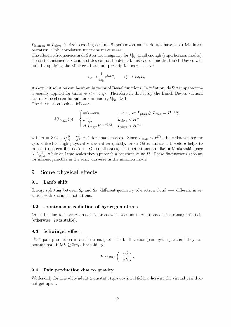
Figure 1: Casimir effect

9.5 Casimir effect

One might ask oneself the question, whether the vacuum energy has any reasonable meaningby itself or if it is just a mathematical relict. In fact, differences in vacuum energy in differentspace-time regions lead to effects that can be measured experimentally. An example is theCasimir effect, an attractive force between two uncharged plates in vacuum, which was indeedexperimentally verified.Consider two plates at a distance L in vacuum in 1 + 1 dimensions. For simplicity, we onlydeal with a scalar field. In experiments, the force between the plates is due to fluctuations ofthe electromagnetic field. We want to solve

∂2t φ− ∂2

xφ = 0

with boundary conditions:

φ(t, x)|x=0 = 0 = φ(t, x)|x=L .

The solutions are standing waves with nodes on the plates. Therefore the frequencies betweenthe plates are no longer continuous (like for a field in a box). Rather, the classical solutionbetween the plates consists only of a superposition of discrete frequencies:

φ(t, x) =

∞∑n=1

(An e−iωnt +Bn eiωnt

)sinωnx,

with ωn = nπL . Quantization gives:

φ(t, x) =

√2

L

∞∑n=1

sinωnx√2ωn

(a−n e−iωnt +a+

n eiωnt).

The prefactor guarantees the right commutation relations. To compute the vacuum energybetween the plates, we need the Hamiltonian:

H =1

2

∫ L

0dx

[(∂tφ)2

+(∂xφ

)2]Some straightforward algebra gives the energy density per unit length:

ε0 =1

L〈0|H|0〉 =

1

2L

∑k

ωk =π

2L2

∞∑n=1

n,

where |0〉 is the Minkowski vacuum defined w.r.t. a±−.Seems, we run into trouble, since the energy turns out to be infinite. This is a standard problem

13

that plagues quantum field theory. Many results diverge, and to extract physical prediction,one has to introduce a regularization method. There are many different regularization schemesin QFT, for example dimensional regularization. Here, instead of d dimensions, we work ind+ε dimensions. The end result contains usually a term divergent in 1

ε . After renormalization,the terms are finite again.We want to apply another method, which might seem even more obscure, namely zeta-functionregularization. The zeta-function is defined for s ∈ C with <(s) > 1 by:

ζ(s) =∞∑n=1

1

ns.

Comparing to our result, we see that the vacuum energy corresponds to s = −1. But thesum representation above is not defined for s = −1. Nevertheless, the zeta-function can beanalytically continued into the complex plane. In particular, the value at s = −1 is well-defined, and turns out to be − 1

12 , giving us a result for the vacuum energy9. The expectationvalue for the energy is negative, which is possible in QFT.The outside region can also be described by our formula above, but now we shift the secondplate to infinity, L → ∞. The difference between the energies per unit length L inside andoutside is:

ε− ε0 =π

2L2

∞∑n=1

n− limL→∞

π

2L2

∞∑n=1

n = − π

24L2.

The energy difference results in the Casimir force

F = − d

dL(ε− ε0) = − π

24L2.

In 3 + 1 dimensions, one gets:F

A= − π2

240L4.

10 The Unruh effect

10.1 Rindler space-time

We follow [4], section 4.5, with slightly different metrics and sign conventions.The Unruh effect deals with an accelerated observer in flat Minkowski space-time. For sim-plicity, we only look at the 2-dimensional case. The relevant metric is Rindler space-time:

ds2R = (aρ)2dτ2 − dρ2.

9 The same argument is used in bosonic string theory to calculate the central charge c of the Virasoroalgebra:

[Lm, Ln] = (m− n)Lm+n +c

12(m3 −m)δm+n.

In the light-cone gauge in D dimensions, the D−2 transverse oscillators contribute to the Hamitonian. Normalordering gives a term (D − 2) 1

2

∑n = −D−2

24(zero-point energy). The contribution from the Faddeev-Popov

ghosts (these guys turn up in the gauge fixing procedure of the path integral) is 1. To avoid a conformalanomaly (non-zero charge), that spoils gauge invariance, the two contributions must cancel. Therefore criticalbosonic string theory is formulated in D = 26 dimensions. In superstring theory, the Faddeev-Popov obey adifferent CFT with different central charge, and the critical dimension is 10.

14

accelerated

observer

x

t

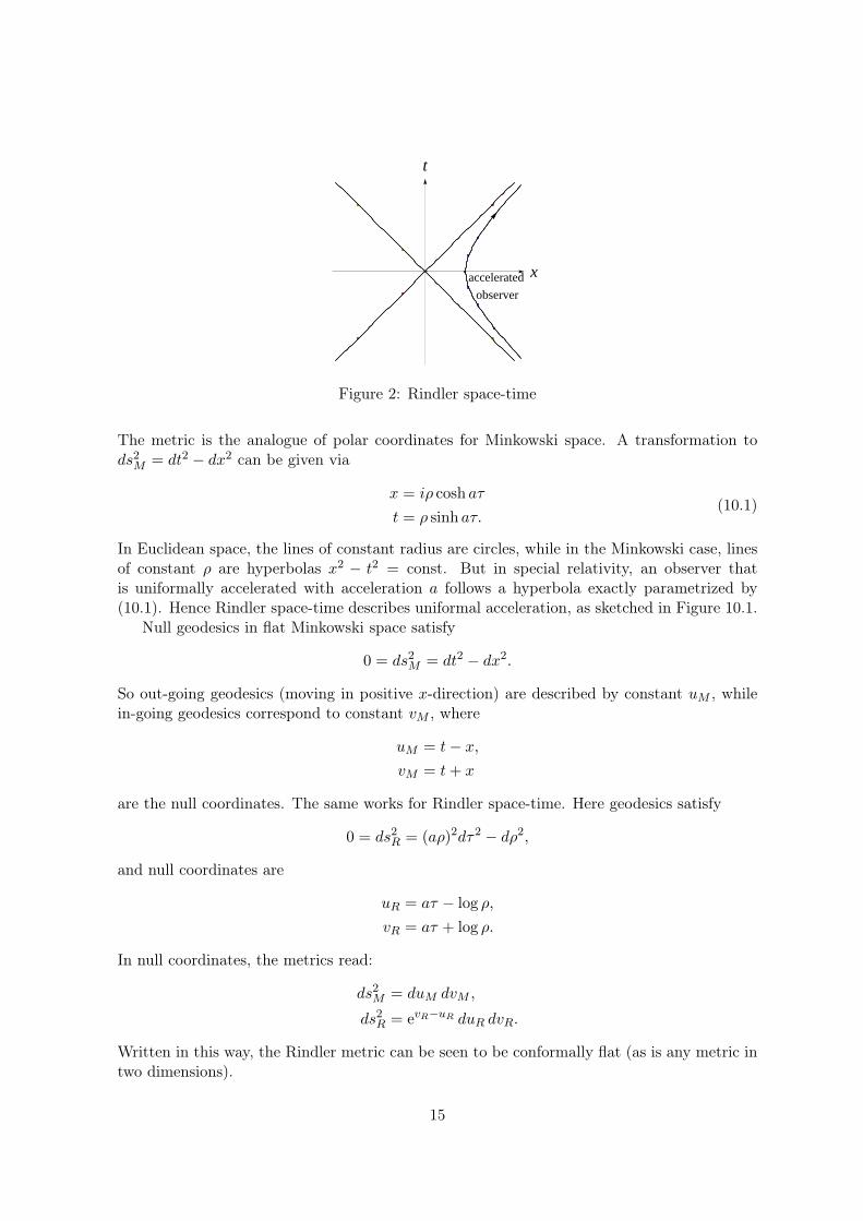
Figure 2: Rindler space-time

The metric is the analogue of polar coordinates for Minkowski space. A transformation tods2M = dt2 − dx2 can be given via

x = iρ cosh aτ

t = ρ sinh aτ.(10.1)

In Euclidean space, the lines of constant radius are circles, while in the Minkowski case, linesof constant ρ are hyperbolas x2 − t2 = const. But in special relativity, an observer thatis uniformally accelerated with acceleration a follows a hyperbola exactly parametrized by(10.1). Hence Rindler space-time describes uniformal acceleration, as sketched in Figure 10.1.

Null geodesics in flat Minkowski space satisfy

0 = ds2M = dt2 − dx2.

So out-going geodesics (moving in positive x-direction) are described by constant uM , whilein-going geodesics correspond to constant vM , where

uM = t− x,vM = t+ x

are the null coordinates. The same works for Rindler space-time. Here geodesics satisfy

0 = ds2R = (aρ)2dτ2 − dρ2,

and null coordinates are

uR = aτ − log ρ,

vR = aτ + log ρ.

In null coordinates, the metrics read:

ds2M = duM dvM ,

ds2R = evR−uR duR dvR.

Written in this way, the Rindler metric can be seen to be conformally flat (as is any metric intwo dimensions).

15

An observer following the hyperbola as sketched in Figure 10.1 can only receive signals fromthe lower quarter, while it can only send signals to the upper quarter. Hence there is no way tosynchronize clocks in these cases and hence no notion of distance. The Rindler metric thereforeonly covers one quarter of Minkowski space. In particular there is a horizon, corresponding tothe boundary of the Rindler wedge x > |t| in Minkowski space time. The horizon consists ofuR =∞ (or uM = 0) and vR = −∞ (or vM = 0).Next we add a second wedge, which we get by reflecting the old one in the origin. The old oneis called R (right), the new one is called L (left). The remaining wedges are called F (future)and P (past).We want to find out the physical implications of the acceleration. Let us quantize a scalarfield as usual, that obeys the Klein-Gordon equation(

∂2t − ∂2

x

)φ = ∂uM∂vMφ = 0.

Since the equation of motion is conformally invariant, in Rindler space it is simply

∂uR∂vRφ = 0.

The solutions are the same as given above in equation (5.2). In Minkowski space, they are:

vMk =1√ωk

eiωt .

In Rindler space, we can solve in R or L respectively:

vR(R)k =

1√ωk

eiω(vR−uR) in R

0 in L

vR(L)k =

0 in R

1√ωk

e−iω(vR−uR) in L

Now vR(R)k is a complete set of solutions in R, while vR(L)

k is complete in L. Furthermore, onecan show, that together they are complete in the whole Minkowski space.The fields can be expanded in either set:

φ =

∫d3k

(2π)3/2

1√2

((vMk )∗ eik·x a−k + vMk e−ik·x a+

k

)=

=

∫d3k

(2π)3/2

1√2

((vR(R)k )∗ eik·x bR−k + v

R(R)k e−ik·x bR+

k + (vR(L)k )∗ eik·x bL−k + v

R(L)k e−ik·x bL+

k

)Now there are two vacuum states:

Minkowski vacuum: a−k |0M 〉 = 0,

Rindler vacuum: bR−k |0R〉 = bL− |0R〉 = 0.

The system must be in the Minkowski vacuum, being the lowest energy state of an inertialobserver. To prepare a state in Minkowski space in the Rindler vacuum, one needs an infiniteamount of energy: if the energy is uniformly distributed in Rindler space, the energy den-sity diverges (after zero-energy subtraction) at the horizon, which corresponds to an infinite

16

coordinate region in Rindler space. This is not sensible, since it would lead to an infinitebackreaction due to Einstein equations.To compute the excitation number, an accelerated observer measures in the Minkowski vac-uum, we have to compute generalized Bogolyubov transformations, i.e. the transformation isno longer diagonal in the momentum. Rather:

d−Ω =

∫ ∞−∞

dω(α(ω,Ω) c−ω + β(ω,Ω) c+

ω

), . . .

The Rindler mode functions must pick up some negative frequency, since they are non-smoothat the horizon, due to the sign flip in the exponent. Therefore, they cannot be superpositionsof the analytic Minkowski mode functions.To do the calculation, we construct two combinations that are analytic and bounded in thelower half planes in uR and vR, namely:

1√2 sinh(πωa )

(uR(R)k + e−

πωa (u

R(L)−k )∗

)1√

2 sinh(πωa )

((uR(R)−k )∗ + e

πωa u

R(L)k

)as one can check in a straight-forward fashion.Expanding in these new mode functions, the corresponding operators must now annihilate theMinkowski vacuum. By taking inner products (φ, u

R(R)k ) and (φ, u

R(L)k ) one gets the needed

Bogolyubov coefficients.Between the accelerated frame and the flat metric, one finds the mean density of particleswith momentum Ω as seen from the accelerator to be:

nΩ =exp

(−πω

a

)2 sinh πω

a

=1

exp(

2πωa

)− 1

.

This corresponds to a Bose-Einstein blackbody radiation of Unruh temperature

T =a

2π.

11 Black holes and thermodynamics

11.1 Basic facts on Black holes

Several solutions for black holes were found. They can be listed by increasing complexity:

1. The first solution found was the Schwarzschild black hole (1916):

ds2 = −(

1− rsr

)dt2 +

1

1− rsr

dr2 + r2dΩ2,

where rs = 2GNM = 3 MM

km is the Schwarzschild radius.It solves the Einstein equations in vacuum Rab = 0, and is

• stationary: there exists a time-like Killing vector field ξa (or a one-parameter groupof isometries φt with time-like orbits).

17

• spherically symmetric: the isometry group contains SO(3).

• static10: the orbits of φt are integrable, meaning there exist hypersurfaces orthog-onal to φt0 for any t0. By Frobenius’ theorem:

ξ[ ∧ dξ[ = 0.

Here ξ[ is the corresponding one-form, which in abstract-index notation is writtenξa = gabξ

a.

2. There exists a further generalization to a charged black hole (Reissner-Nordström met-ric):

ds2 =

(1− rs

r+e2

r2

)dt2 − dr2

1− rsr + e2

r2

− r2dΩ2,

with r2 = 2GNM as above.

3. The most general metric is the Kerr metric, describing a rotating, charged black hole:

ds2 =− ∆− a2 sin2 θ

Σdt2 − 2a(r2 + a2 −∆) sin2 θ

Σdt dφ+

+(r2 + a2)2 −∆ a2 sin2 θ

Σsin2 θ dφ2 +

Σ

∆dr2 + Σ dθ2,

Σ =r2 + a2 cos2 θ,

∆ =r2 + a2 + e2 − 2Mr.

To avoid naked singularities (which should be forbidden according to the Cosmic Cen-sorship Conjecture), one requires:

e2 + a2 ≤M2, (11.1)

so for a given mass, a black hole cannot have an arbitrarily high charge, or cannot rotatearbitrarily fast. If equality holds, the black hole is called extremal.

11.2 Hawking radiation

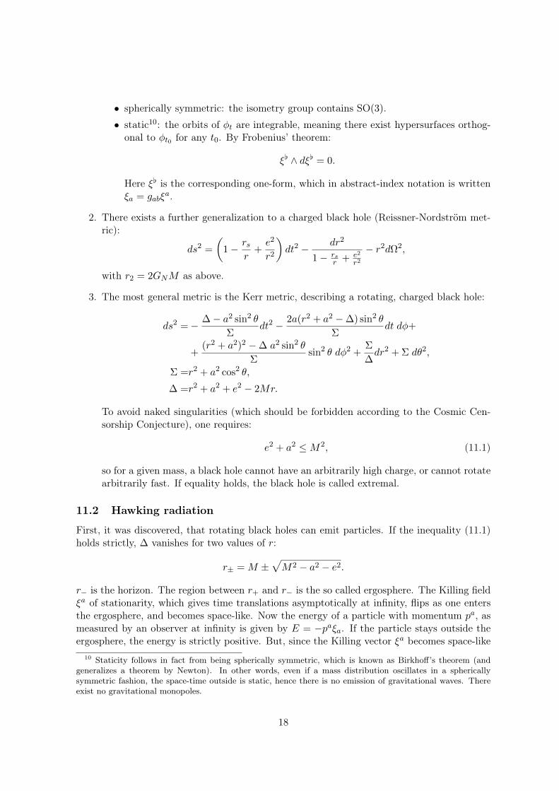
First, it was discovered, that rotating black holes can emit particles. If the inequality (11.1)holds strictly, ∆ vanishes for two values of r:

r± = M ±√M2 − a2 − e2.

r− is the horizon. The region between r+ and r− is the so called ergosphere. The Killing fieldξa of stationarity, which gives time translations asymptotically at infinity, flips as one entersthe ergosphere, and becomes space-like. Now the energy of a particle with momentum pa, asmeasured by an observer at infinity is given by E = −paξa. If the particle stays outside theergosphere, the energy is strictly positive. But, since the Killing vector ξa becomes space-like

10 Staticity follows in fact from being spherically symmetric, which is known as Birkhoff’s theorem (andgeneralizes a theorem by Newton). In other words, even if a mass distribution oscillates in a sphericallysymmetric fashion, the space-time outside is static, hence there is no emission of gravitational waves. Thereexist no gravitational monopoles.

18

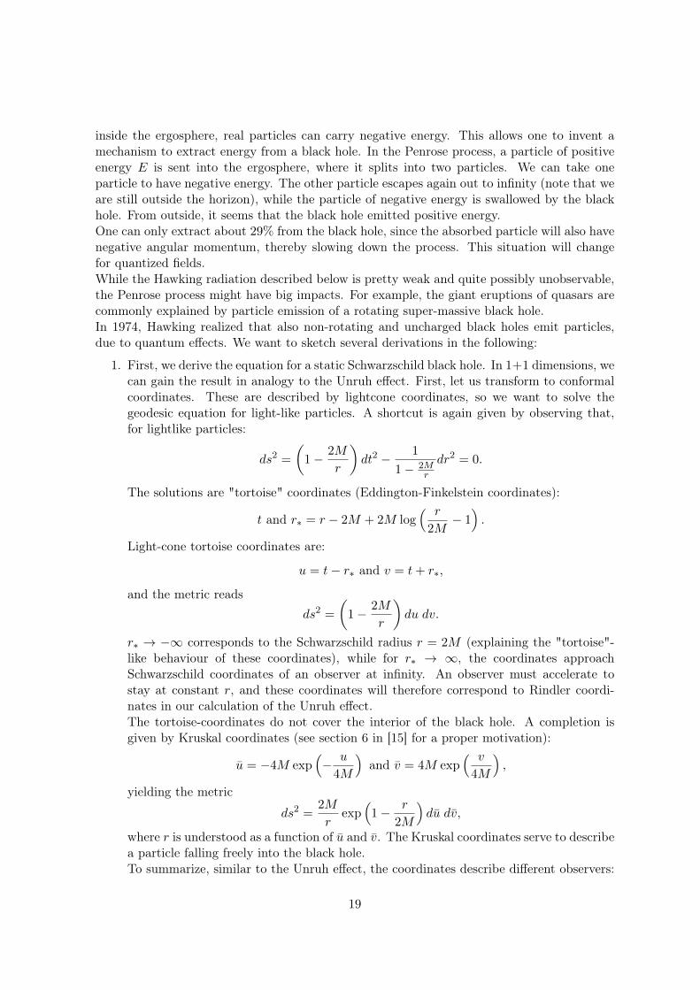
inside the ergosphere, real particles can carry negative energy. This allows one to invent amechanism to extract energy from a black hole. In the Penrose process, a particle of positiveenergy E is sent into the ergosphere, where it splits into two particles. We can take oneparticle to have negative energy. The other particle escapes again out to infinity (note that weare still outside the horizon), while the particle of negative energy is swallowed by the blackhole. From outside, it seems that the black hole emitted positive energy.One can only extract about 29% from the black hole, since the absorbed particle will also havenegative angular momentum, thereby slowing down the process. This situation will changefor quantized fields.While the Hawking radiation described below is pretty weak and quite possibly unobservable,the Penrose process might have big impacts. For example, the giant eruptions of quasars arecommonly explained by particle emission of a rotating super-massive black hole.In 1974, Hawking realized that also non-rotating and uncharged black holes emit particles,due to quantum effects. We want to sketch several derivations in the following:

1. First, we derive the equation for a static Schwarzschild black hole. In 1+1 dimensions, wecan gain the result in analogy to the Unruh effect. First, let us transform to conformalcoordinates. These are described by lightcone coordinates, so we want to solve thegeodesic equation for light-like particles. A shortcut is again given by observing that,for lightlike particles:

ds2 =

(1− 2M

r

)dt2 − 1

1− 2Mr

dr2 = 0.

The solutions are "tortoise" coordinates (Eddington-Finkelstein coordinates):

t and r∗ = r − 2M + 2M log( r

2M− 1).

Light-cone tortoise coordinates are:

u = t− r∗ and v = t+ r∗,

and the metric readsds2 =

(1− 2M

r

)du dv.

r∗ → −∞ corresponds to the Schwarzschild radius r = 2M (explaining the "tortoise"-like behaviour of these coordinates), while for r∗ → ∞, the coordinates approachSchwarzschild coordinates of an observer at infinity. An observer must accelerate tostay at constant r, and these coordinates will therefore correspond to Rindler coordi-nates in our calculation of the Unruh effect.The tortoise-coordinates do not cover the interior of the black hole. A completion isgiven by Kruskal coordinates (see section 6 in [15] for a proper motivation):

u = −4M exp(− u

4M

)and v = 4M exp

( v

4M

),

yielding the metric

ds2 =2M

rexp

(1− r

2M

)du dv,

where r is understood as a function of u and v. The Kruskal coordinates serve to describea particle falling freely into the black hole.To summarize, similar to the Unruh effect, the coordinates describe different observers:

19

(a) Eddington-Finkelstein coordinates

Black Hole

White Hole

(b) Kruskal coordinates

• Kruskal coordinates: locally inertial (freely falling) observers. The correspondingvacuum is |0K〉.• Tortoise coordinates: observers at constant r (they must accelerate to stay at a

fixed position). Vacuum: |0T 〉.

Again the Bogolyubov coefficient are calculated, as above. The proper acceleration isgiven by a = 1

4M , leading to the Hawking temperature:

TH =~c3

Gk· 1

8πM∼M2p

M.

Unruh and Hawking effect are quite similiar in two dimensions:

Unruh Hawkinginertial observer ("free fall" in flatspace): |0M 〉

free-fall observer: |0K〉

accelerated observer: |0R〉 observer at constant r (acceleratedin curved space): |0T 〉

T = 12π a T = 1

8π1M

With massive fields, the particle density is given by:

n =1

exp(ETH

)− 1

,

with E =√m2 + k2 which is only large enough for small masses. Radiation of massless

particles is exponentially suppressed.In 3+1 dimensions, one must include a greybody factor < 1 accounting for a barrier-likepotential in the Laplace equation.

2. Hawking’s original derivation [9] of the black hole radiation was somewhat different. Hedid not consider an eternal Schwarzschild black hole, but instead he looked at mattercollapsing to a black hole. Intuitively, black hole evaporation can be understood ashighly energetic particles staying close to the horizon for a long time. Eventually, they

20

can escape and reach the detector. Though the two approaches seem to desribe differentphysical setups (in the first case, an eternal black hole emitting particles, in the seconda black hole forming), they give the same result, namely a black body radiation withHawking temperature.

3. Another, more heuristic interpretation goes as follows: consider a pair of particles, onewith positive, the other with negative energy. The latter can tunnel through the eventhorizon. Inside the black hole, the time-like killing vector field turns space-like, andhence the particle becomes real (now propagating time-like). The particle of positiveenergy can propagate to infinity. The probability of this effect to happen is proportionalto the surface gravity, the area of the black hole horizon.This explanation resembles the Penrose process described above. But note that theHawking effect is a pure quantum effect. The Penrose process happens outside theBlack hole horizon. For non-rotating black holes, the Killing vector flips only inside thehorizon, and a splitting procedure as for the Penrose process cannot work, since there isno way that one particle can again escape to infinity.

4. Finally, there is a very elegant and short derivation, to get the temperature from themetric. We follow [3], page 562.A thermodynamical system can be completely described (in the canonical ensemble) byits partition function:

Z = Tr e−βH ,

where β = 1kBT

. In the following, we fix kB = 1. Statistical mechanics can be dis-cribed very laxly as a quantum field theory in Euclidean time. In quantum mechanics,time-evolution is given by e−iHt. The partition function above can be understand as atheory with Euclidean time compactified on a circle. Taking the trace means, time iscompactified on a circle of length β.First we have to compute the analytic continuation of the Schwarzschild metric, byreplacing t → iτ . Now, at the horizon, the metric has to be regular at the horizon.Therefore expand, close to the horizon: r = rs(1 + ρ2). The metric transforms to:

ds2 = 4r2s

(dρ2 + ρ2

(dτ

2rs

)2

+1

4dΩ2

).

This is a metric of a flat plane (times a sphere), provided that τ is an angular parameterwith period 2rs = β = 1

T .

11.3 Thermodynamics

A first hint to the thermodynamical behaviour of black holes was the area theorem, whichstates, loosly speaking, that the area of the horizon surface of a black hole can never decreasein time. For the general formulation and a proof, see Theorem 12.2.6 of [15].Replacing the area by an entropy, we get the second law of thermodynamics.Indeed, having derived the Hawking temperature, we can compute the Bekenstein entropy ofblack holes:

SBH =

∫dE

T=

∫dM

T=

1

44π(2M)2 =

1

4A,

21

using the black hole radius rs = 2M .Stefan-Boltzmann’s law11:

L = γσT 4HA,

leads to:

M = −∫dtL = M0

(1− t

tL

)1/3

, tL = 5120πM3

0

γ,

and hence leads to a finite life-time tL (without quantum gravity effects)12.Black holes have negative heat capacity

CBH =∂E

∂T=∂M

∂T= − 1

8πT 2,

so they become colder, if they absorb mass and energy. This is a very interesting property,we want to explore a bit further.

11.3.1 Detour: entropy

An excellent overview is given in chapter 27 of Penrose’s epic book [14].Entropy is a coarse graining phenomenon. Divide the phase space into several regions, suchthat all states within such a region have the same macroscopic behaviour. Define the entropyof a state by

S = kB log V,

where V is the volume of the region the state belongs to. Of course there is some arbitrarinessin the definition, since different observers might disagree about what are macroscopicallyindistinguishable states. Nevertheless, thanks to the logarithm, the differences are ridiculouslysmall. Now a state in thermal equilibrium corresponds to a state of highest entropy, containedwithin the largest volume in the phase space. The second law seems intuitively clear: if we arein a state in a small volume, it is highly likely that we will end up in a state of higher entropy(higher volume) after some time, until finally we are in the biggest box (maximal entropy,thermal equilibrium). In other words: entropy never decreases.There is a subtle point underlying these hand-waving arguments: our state must be in a smallvolume (low entropic state) to begin with. We would not even exist in thermal equilibrium.Let’s aks the question, how can we do anything at all? To tidy up my room, the entropy ofmy room decreases, hence my own entropy must increase, to get a gain in entropy in the end.How does it work? We owe all that to the sun, being a "hot spot in a cold universe". Duringthe day, the sun sends us highly-energetic photons. At night, the earth emits again all theenergy, but now in form of photons of low energy. There are much more of these, hence moredegrees of freedom, hence higher entropy (larger volume in phase space). So only, because theenergy from the sun has a very low entropy, plants can use it to decrease their own entropy,while we eat plants to decrease our own.So how can the sun emit low entropy photons? The reason lies in the peculiar interplay ofgravitation and entropy:

• A gas is in thermal equilibrium, if it is spread all over a given volume.

11 L: flux of energy, γ: degrees of freedom, σ = π2

60: Stefan-Boltzmann constant.

12 Only for very light black-holes, the life-time is small w.r.t. the age of the universe.

22

TunnelingΦ

V

(c) Old inflation

Φ

V

(d) New inflation

Φ

V

(e) Chaotic inflation

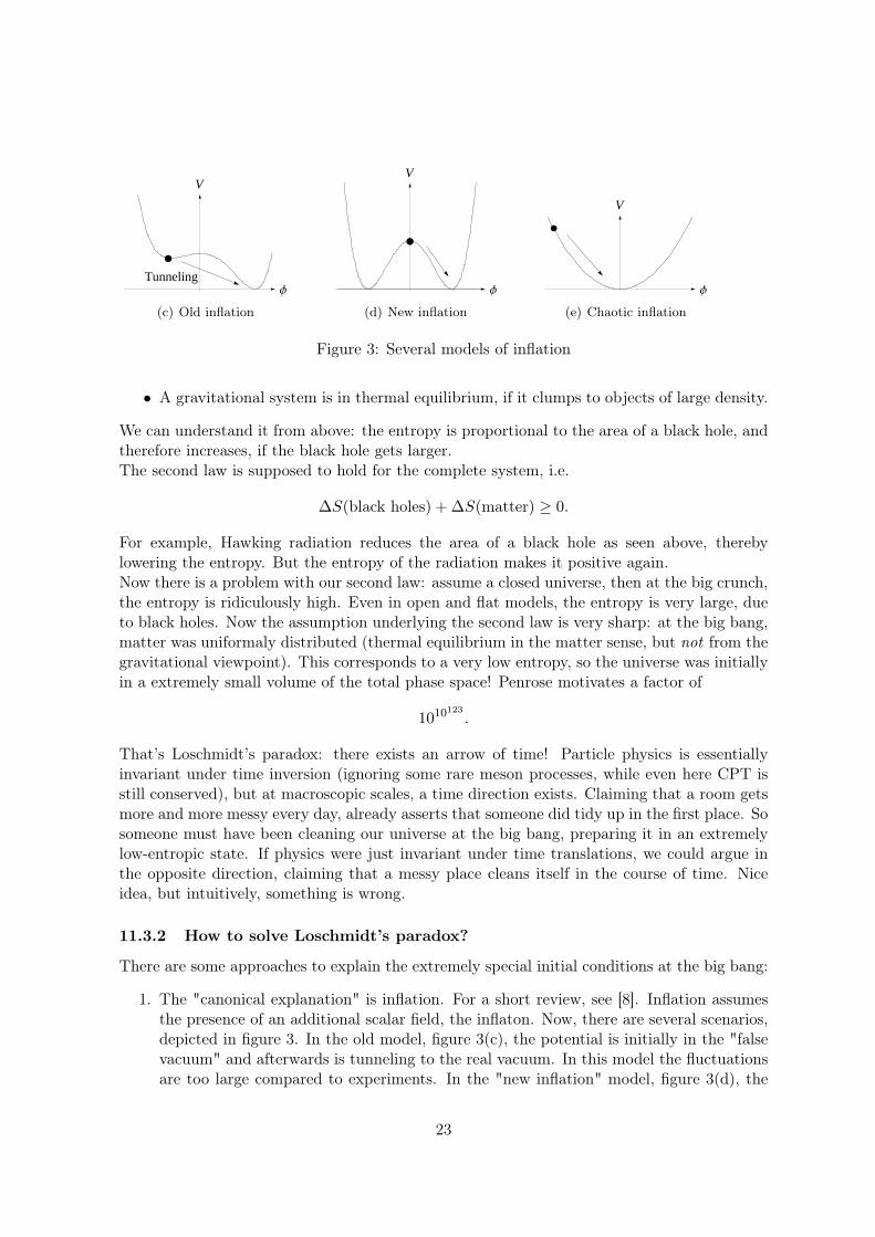
Figure 3: Several models of inflation

• A gravitational system is in thermal equilibrium, if it clumps to objects of large density.

We can understand it from above: the entropy is proportional to the area of a black hole, andtherefore increases, if the black hole gets larger.The second law is supposed to hold for the complete system, i.e.

∆S(black holes) + ∆S(matter) ≥ 0.

For example, Hawking radiation reduces the area of a black hole as seen above, therebylowering the entropy. But the entropy of the radiation makes it positive again.Now there is a problem with our second law: assume a closed universe, then at the big crunch,the entropy is ridiculously high. Even in open and flat models, the entropy is very large, dueto black holes. Now the assumption underlying the second law is very sharp: at the big bang,matter was uniformaly distributed (thermal equilibrium in the matter sense, but not from thegravitational viewpoint). This corresponds to a very low entropy, so the universe was initiallyin a extremely small volume of the total phase space! Penrose motivates a factor of

1010123.

That’s Loschmidt’s paradox: there exists an arrow of time! Particle physics is essentiallyinvariant under time inversion (ignoring some rare meson processes, while even here CPT isstill conserved), but at macroscopic scales, a time direction exists. Claiming that a room getsmore and more messy every day, already asserts that someone did tidy up in the first place. Sosomeone must have been cleaning our universe at the big bang, preparing it in an extremelylow-entropic state. If physics were just invariant under time translations, we could argue inthe opposite direction, claiming that a messy place cleans itself in the course of time. Niceidea, but intuitively, something is wrong.

11.3.2 How to solve Loschmidt’s paradox?

There are some approaches to explain the extremely special initial conditions at the big bang:

1. The "canonical explanation" is inflation. For a short review, see [8]. Inflation assumesthe presence of an additional scalar field, the inflaton. Now, there are several scenarios,depicted in figure 3. In the old model, figure 3(c), the potential is initially in the "falsevacuum" and afterwards is tunneling to the real vacuum. In this model the fluctuationsare too large compared to experiments. In the "new inflation" model, figure 3(d), the

23

false vacuum is on a plateau and the inflaton rolls down the potential. In the thirdmodel, "chaotic inflation", figure 3(e), no plateau is needed, and the inflaton starts ina generic point and rolls down the potential. The inflaton serves as a force to drive aninflation of space-time, hence the name. The force is given by:

dW = −p dV = ρdV

where the last expression is the energy of the expanded matter. Assuming a FLRWspace-time13:

a = −4π

3(ρ+ 3p)a =

8π

3ρa.

leading to an exponential expansion:

a ∼ eξt , with ξ =

√8π

3ρ.

ξ−1 sets a time-scale for inflation, called an e-folding.In the new inflation and the chaotic inflation models, so-called "internal inflation" canset in. The decay of the false vacuum is an exponential process, just as inflation itself.In fact inflation can be even stronger, so always a portion of the original space remainsin the false vacuum, starting inflation again. Lots of baby universes evolve.In principle this is a dangerous result, making it hard to make any predictions at all.Nevertheless, it might be a criterion to rule out vacua in M-theory of string theory.Vacua leading to stronger inflation will dominate, even if they have a lower a prioripossibility.Now the history of the universe is as follows:

• The universe is initially in a chaotic state.• If some small patch was in the false vacuum, this patch gets inflated as the infla-

ton rolls down the potential. Here false vacuum denotes the minimum in the oldinflation model, the plateau in the new model or a state of high expectation value(due to quantum fluctuations) in the chaotic model.• When the inflaton is in the true minimum of the potential, inflation stops.• The inflaton couples to other particles and therefore its energy gets converted to a

"hot soup" of particles.• Now we are at the hot big bang, and the standard model of cosmology sets in.

Inflation served to solve several problems:

(a) It explains, why the universe is large. After about 60 e-foldings, the particle contentof at least 1090 baryons can be explained.

(b) It explains, why the universe is isotropic and homogeneous. All of the visible uni-verse started in a small patch, which thermalized (in the radiation sense, not in thegravitational sense!). This explains the properties of the cosmic microwave back-grounds. Inflation of quantum fluctuations of the potential even serve to describethe fine-structure of the CMB (small anisotropy).

13 this result should also hold in more general initial space-times, according to the cosmological "no-hair"conjecture.

24

(c) It explains the flatness of the universe. Flatness occurs, if the density of the universeis critical. In cosmological models:

ρ

ρcrit=

1 + const · t radiation-dominated1 + const · t2/3 matter-dominated1 + const · e−2Ht inflation

Only inflation serves to drive the value towards 1.

(d) GUT theories predict topological defects (monopoles, cosmic strings, domain walls).The energy density of monopoles would completely dominate the universe, whichis unobserved. Inflation solves the monopole problem, by diluting the monopoledensity. Inflation must set in after monopole formation.

2. If Penrose’s argumentation above is true, there must be at least some doubt on themotivation of inflation. Inflation tries to explain the homogeneity due to thermalizationeffects (matter can interact until it gets inflated apart). But thermalization increasesthe entropy, so the universe must have been even more special before.An alternative idea, due to Penrose, is the Weyl curvature conjecture that states, thatat the big bang the Weyl curvature did vanish. Loosely speaking, curvature can be splitinto a Ricci and a Weyl part:

• Ricci curvature "contracts". Consider the effect of a massive object on a sphere oftest mass surrounding it. It will be contracted spherically symmetric towards theobject. Ricci curvature also enters Einstein’s equations.

• Weyl curvature is "tidal". Consider a little sphere outside a massive object. Differ-ent parts of the sphere get attracted with different strength, leading to tidal effects(compare moon/earth)! Weyl curvature also appears in the presence of gravita-tional waves.

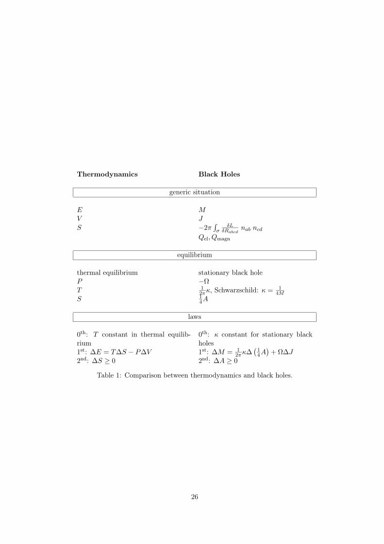
11.4 Laws of black hole thermodynamics

1. Zeroth law: for a body in thermal equilibrium the temperature is constant. For blackholes, this generalizes to the fact that for stationary black holes, the surface gravity κis constant over the event horizon. Some notions have to be explained:

• The future horizon h+ is the boundary I−(⋃

γ), where the union goes over all

geodesics tangent to Killing vector fields in the region outside the black hole. I−(γ)is the set of points that can be joint to γ by time-like future-directed curves endingon γ (for more precise definitions, see chapter 5.3 in [16]).

• Look at a black hole with stationary Killing vector field ξa. If the black hole isrotating, ξa is in general not normal to h+. Rather there exists a second Killingvector field χa, which can be written as:

χa = ξa + Ωφa,

where ξaξa → −1 at infinity, and φa is a field with closed orbit, normalized toperiod 2π. Here, Ω is the angular velocity of the horizon.

25

Thermodynamics Black Holes

generic situation

E MV J

S −2π∫σ

δLδRabcd

nab ncdQel, Qmagn

equilibrium

thermal equilibrium stationary black holeP −ΩT 1

2πκ, Schwarzschild: κ = 14M

S 14A

laws

0th: T constant in thermal equilib-rium

0th: κ constant for stationary blackholes

1st: ∆E = T∆S − P∆V 1st: ∆M = 12πκ∆

(14A)

+ Ω∆J2nd: ∆S ≥ 0 2nd: ∆A ≥ 0

Table 1: Comparison between thermodynamics and black holes.

26

• On h+, we have χbχb = 0, and therefore ∇a(χbχb) is normal to h+. χa is also itselfnormal to the Killing surface, and therefore they are proportional:

∇a(χbχb) = −2κχa,

the proportionality constant is the surface gravity. χa is a Killing vector, satisfying∇(aχ b) = 0. So we can rewrite:

χb∇bχa = κχa, (11.2)

a nonaffinely parametrized geodesic equation. For a Schwarzschild black hole, κ =1

4M . The surface gravity generalizes the well-known surface gravity of the earthg = GM

r2 .

2. First law: ∆E = T∆S − P∆V . For black holes, one gets: ∆M = 12πκ∆

(14A)

+ Ω∆J .We want to outline the proof of this formula, and refer for details to [15] and [16]. LetN be the event horizon of a black hole, or more generally a null hypersurface. Letka be tangents to null geodesic generators, parametrized affinely with parameter λ, sokaka = −1. Define the following quantities:

hab = gab + kakb spatial metric

Bab = ∇bka = σab + ωab +1

3θ hab

θ = habBab expansion

σab = B(ab) −1

3θ hab shear

ωab = B[ab] twist

To get more intuition, look at a family of geodesics γa. The tensor Bab measures how

an observer on a geodesic γ0 sees geodesics nearby. They get stretched and rotated byBa

b. Expansion measures how they spread, and similiarly for shear and twist. If θ > 0,the geodesic run towards each other, if θ < 0, they get separated. θ fulfills the equationθ = 1

AdAdλ .

Now, Raychaudhuri’s equation hold:

dθ

dλ= −1

3θ2 − σabσab + ωabω

ab −Rabkakb. (11.3)

Proof.

kc∇cBab = kc∇c∇bka = kc∇b∇cka +Rcbadkckd =

= ∇b(kc∇cka)− (∇bkc)(∇cka) +Rcbadkckd =

= 0−BcbBac +Rcba

dkckd.

Tracing, the left-hand side gives ka∇aθ = dθdλ , while the right-hand side gives (using the

orthogonal decomposition above):

−1

9θ habh

ba − σabσba − ωabωba −Rcdkckd.

27

Now let us take a stationary black hole and alter it by an infinitesimal physical process,such that the black hole is not destroyed, but stationary again.To first order in ∆Tab, we neglect σab, ωab, and θ. Einsteins equation yields:

dθ

dλ= −8π∆Tabk

akb. (11.4)

Further:ka =

(∂

∂λ

)a=

1

κλ

∂

∂v=

1

κλχa =

1

κλ(ξa + Ωφa).

Here v is the Killing parameter, such that χa∇av = 1, while λ is the affine parameter.Indeed, the definition ka = e−κvχa gives, with help of equation (11.2):

kb∇bka = e−2κv(χb∇bχa − χaχb∇b(κv)

)= 0.

Therefore(∂∂λ

)a= e−κv

(∂∂v

)a, or λ = eκv, justifying the intermediate step.We multiply (11.4) with κλ and integrate over horizon. Using θ = 1

AdAdλ , the left-hand

side gives:

κ

∫ ∞0

dλ

∫d2S λ

dθ

dλ= κ

∫d2S θλ|∞0 − κ

∫d2S

∫ ∞0

dλ θ = 0− κ∆A.

The right-hand side is evaluated to:

−8π

∫ ∞0

dλ

∫d2S ∆Tab (ξa + Ωφa) kb = −8π(∆M − Ω∆J),

proving the first law.

3. Second law: in a closed system, entropy never decreases, ∆S ≥ 0. For Black holes, thearea of the event horizon never decreases, ∆A ≥ 0. Since the expansion of null-geodesicgenerators of the event horizon of a black hole can be written as θ = 1

AdAdλ , it measures an

increase of the area. An assumption needed for the proof, is the null energy condition:

Tabkakb ≥ 0.

Einstein’s equations lead to Rabkakb ≥ 0, and Raychaudhuri’s equation (11.3) gives:

dθ

dλ≤ −1

2θ2. (11.5)

It follows:1

θ≥ 1

θ0+

1

2λ.

Now, assume the convergence is negative. If the geodesic can be extended far enough,one gets θ(λ) = −∞ for some λ ≤ 2

|θ0| . This cannot happen, as long since the horizonis achronal (see chapter 9 of [15]). A set S is called achronal, if there exist no p, q ∈ S,such that p ∈ I+(p).

The analogy between the laws of thermodynamics and the laws of black holes are summed upin table 1.

28

12 The holographic principle and String Theory

For nice papers and reviews, see [10, 5], and for a textbook covering the information paradoxand the holographic principle, see [12].

12.0.1 Problems and Paradoxa

In the holographic picture, a particle falling into the black hole leaves a fingerprint on thearea of the black hole, storing information about its position and mass. Information is notlost, but rather stored holographically on the black hole horizon. Also the Hawking radiationis not completely black. The principle was motivated by several problems one runs into byapplying only the machinery described above, namely QFT in a classical curved background:

1. A first hint to the holographic principle can be seen from the fact that entropy is propor-tional to the surface, and not the volume. At Planckian scales, the degrees of freedomare not 3 + 1 dimensional, but rather two-dimensional Boolean variables on a two-dimensional lattice. At the Planck scale a physical state corresponds to a basis vectorin a Hilbert space. While at large scales quantum mechanics is described by a superpo-sition of states, at the Planck scale they become irrelevant.The entropy of black holes

S =1

4A = 4πM2

describes not only the metric, but also all quantum fields in its neighbourhood.Let us analyze the problem in more detail: conventional quantum field theory is a localtheory. In the example of a Klein-Gordon field, to every space-time point, an harmonicoscillator is assigned. Let us estimate the degrees of freedom. First, to get a finiteresult, let us assume that QFT is only well-defined down to the Planck-scale, where anew theory of quantum gravity must set in. Therefore, let us assume that space-time iscoarse-grained, such that degrees of freedom can only be assigned to Planckian volumes.We also cut off the harmonic oscillator spectrum at the Planck mass; let us say thereare n states in the spectrum. The number of independent quantum states is nV , whereV is the volume in Planckian units. The degrees of freedom are given by

N ∼ log nV = V log n & V.

Collapsing the system into a black hole via the so-called Susskind-process, the entropyis bounded by the black hole entropy ∼ A. Since we can make the volume V in principlelarger than A it seems that we decreased the entropy in contrast to the generalizedsecond law. Local QFT seems to overcount degrees of freedom. In fact, consider asystem of size of the Planckian volume, containing energy. If we don’t want it to bealready a black hole, its mass must be below the Planck length:

m . lP .

Now, combine N of these systems to a ball of radius R (in Planckian units). Naively, inQFT:

M . N lP =R3

l3PlP =

R2

l2PR.

29

But, again, if we do not want the system to be a black hole, we need:

M . R.

For a ball of radius 1 cm, we get a number of degrees of freedom of 1099 instead of 1033,a clear overcount. String theory helps out here, since strings are extended objects, andtherefore non-local. This makes an implemenation of the holographic principle possible,like in AdS/CFT, as we will see below.

2. In classical general relativity, unitarity seems to be violated. Due to the no-hair theo-rem, black holes are described by only three parameters, massM , charge Q, and angularmomentum a. If a particle falls into a black hole, its information is lost. As we haveseen above, Schwarzschild radiation has a black-body spectrum, and therefore maximalentropy (no information). The opinions about the fate of black holes differ, some (likeStephen Hawking) favour a complete loss of information, others (like Leonard Susskind)prefer conservation of information (Susskind refers to these discussions as the "Blackhole wars"). Recent progresses, mainly due to String-Theory-inspired AdS/CFT, seemto point into the second direction. AdS/CFT claims a duality between a certain gravi-tational theory and a conformal field theory. In particular, the latter is unitary, so thefirst must be unitary as well. It is not possible to loose information in black holes. Wesay more about this later on. Let us from now on assume that quantum mechanics hold,namely that information is stored, and all processes are unitary.

3. The entropy can be calculated not only via the first law of black hole thermodynamics,but also directly from the QFT and the Hawking temperature. In the calculation theentropy is cut-off dependent and diverges at the horizon. This is again an indication ofan over-counting of local QFT.

4. In quantum mechanics, it is forbidden to copy information. Let a test-particle (i.e.yielding no big back-reaction) fall into a black hole. If Hawking radiation carries in-formation about the particle, it must be possible for a second observer to store thisinformation, then fall itself into the black hole, and meet the first particle again. It hascopied information, in contrast to the Xeroxing principle.

5. Baryon number is not preserved, when a particle falls into a black hole.

12.1 Black hole complementarity

To overcome these problems, several steps forward have been taken. Black hole complemen-tarity is the assertion that the laws of physics are valid for all observers. Let us consider againthe problem of Quantum Xeroxing, as described above. The solution of the paradox is quitesubtle, but shows, how a black hole "cares about" the laws of nature. First, we have to knowa little bit more about information and entropy. Let us look at a system S, described by adensity matrix ρ. It consists of several subsystems Si with respective density matrices ρi.There are several definitions that become relevant:

1. Von-Neumann entropy (fine-coarsed entropy):

S(S) = −Tr ρ log ρ.

Von-Neumann entropy is not additive.

30

2. Thermal entropy (coarse grained entropy):

Sthermal(S) =∑

S(Si).

The entropy is by definition additive.

3. Information is defined by:

I(S) = Sthermal(S)− S(S),

and is usually measured in bits.

To understand the difference between the two entropies, consider a system in a pure state. TheVon-Neumann entropy will vanish, since Tr ρ = 0. The subsystems nevertheless get entangled,and in general the respective entropies will be non-vanishing. Looking only at one subsystem,and forgeting the others, more states look the same. In this way, information gets lost at largescales (via thermal coarse graining), while it is still retained microscopically (von-Neumannentropy).

Now, interestingly, systems smaller than half the complete system, carry less than one bit,i.e. for Σi <

12Σ:

S(Si) ∼= Sthermal(Si),

I(Si) ∼= 0.

Therefore, the observer outside the black hole must wait, until the black hole evaporated tohalf its size until it gets any information at all! Here comes the problem: in order to providea possiblitiy for the two observers to meet again inside the black hole, the first particle mustaccelerate against the attraction of the black hole for a long time in order not to fall into thesingularity. But this requires an amount of energy so big, that the observer is a black holeby itself. The situation changes completely, and our assumptions, that the observers are only"test-particles" is no longer valid. The black hole does not allow Quantum Xeroxing thateasily and the paradoxon no longer exists!

Baryon number violation receives a similar solution. There must be some process in natureviolating baryon number in order to explain the excess of baryons over anti-baryons which mustresult from processes in the early universe. Possible sources are sphalerons (non-perturbativeeffects within the standard model), or massive particles coupling baryons to anti-baryons orleptons, as occur naturally in GUT-theories. For example, assume a pXe+ coupling, i.e. aninteraction between a proton, a positron and a field X with large mass mX . The particle isassumed to be massive, so the process was relevant only at higher energies in an earlier stageof the universe. This interaction leads to proton decay (as predicted in GUT theories). Theseprocesses are always present, but for a observer in the rest frame of the proton, the oscillationsoccur on time scales 1

mXwhich are extremely small, so time-averaged, the proton is stable (as

observed in nature). Nevertheless, now let the proton cross the horizon of a black hole. Fromfar away, it takes infinite time for the particle to approach the horizon. Now let there be anoscillation from proton to a positron. From far away it takes an infinite time to get back theoriginal proton state; the proton seems to have decayed. This is also expected, since fromfar away, the proton is inside a heat bath (due to Hawking radiation), that provides energy

31

for creation of X particles. The processes look completely different for the two observers,nevertheless no physical laws are violated14!

It is common to define the stretched horizon, i.e. a small deformation of the horizon awayfrom the singularity. In AdS/CFT this is quite naturally. Here AdS5 comes naturally witha boundary. On the boundary a CFT is defined on a stack of D-branes. The scatteringamplitudes of strings off D-branes can be calculated and yield an effective thickness of the D-branes, some sort of open string halo. The stretched horizon serves to cut off some singularities.

The stretched surface has interesting properties. If a charged particles falls across thestretched surface, the surface acts as a conductor obeying Ohm’s law! From the point of viewof an observer outside, the charge density gets distributed quickly over the surface, while forthe particle falling freely, nothing special happens. For details, compare chapter 7 in [12].

12.2 The holographic principle

Crudely speaking, the holographic principle states that all entropy contained in some volumecan be stored on its boundary. Of course this definition is much to vague, but it can besharpened to agree with all reasonable physical effects and space-times!

A first guess is to take space-like volumes and claim that the entropy is bounded by theentropy on the boundary. However this cannot work. For example consider a closed universe.Then we can take the volume arbitrarily large, such that the boundary gets arbitrarily small.

A more refined definition is needed. In fact, the bound that seems to hold is the covariantentropy bound: the entropy of any light-sheet of a given space-like surface B is bounded bythe area of B:

S(L(B)

)≤ A(B)

4.

The notion of a light-sheet has to be explained. Consider any space-like surface B. It possessesfour orthogonal null directions, future-directed or past-directed as well as ingoing of outgoing.As a shorthand, we call them (±,±), where the tuple corresponds to time and direction (t, r),+ denoting future-directed, or outgoing respectably, while − corresponds to past-directed, oringoing. We have seen in equation (11.5), that under the null-energy condition Tabkakb ≥ 0(stating that matter has an effect of focusing on light-rays, rather than anti-focusing), nullgeodesic run together, ending at so called caustics, given that the expansion θ is negative atsome point (this is referred to the focussing theorem). Now, at least two null directions havenon-positive expansion. As an example, consider a spherical room, with light-bulbs all overthe wall, both inside and outside. Now switch on the light for a second. The light will runtowards the center of the room, where the light-rays intersect (in-going), and similarly, lightruns of to infinity (out-going). Similarly, the process can be looked at backwards in time.The null directions of negative expansions are (+,−) and (−,+). These directions of negativeexpansion span the light-sheet, ending at caustics (in the example above, the cone towards thecenter of the room, ending on the wall, in both time directions). The problem of the closeduniverse is circumvented, since null directions only converge into the smaller volume.

14 This is analogous to our intuitive explanation of the Hawking process: while usually particle/anti-particlecreation occurs on very tiny scales, if the particle runs outside the horizon, and the anti-particle inside thehorizon back in time, from outside it takes an infinite amount of time until annihilation. Effectively, a particlewas created.

32

12.3 AdS/CFT

We want to give a short glimpse at AdS/CFT and its relation to holography. From the stringtheory point of view, one considers a stack of N coincident D3-branes located in 10 dimensions.These branes are 3 + 1 dimensional objects, where open strings can end. They can be chargedunder fields in the Ramond-Ramond sector of superstring theory. Branes can serve to describeblack holes in string theory. If two open string excitations collide on the brane volume, theymay combine into an open string that can escape away from the brane, leading to Hawkingradiation. One can solve the equations of motion for the background metric in the supergravityapproximation (small string coupling). The metric turns out to be

ds2 = H−1/2p

(− dx2

0 + . . .+ dx23

)+H1/2

p (dr2 + r2dΩ25

).

The first part corresponds to the metric on the D3 brane, while the second part describes themetric in the 10− 4 = 6 dimensions transversal to the brane, written in spherical coordinates,so dΩ2

5 is the metric of an S5. The function relating the two metrics is:

1 +

(R

r

)4

.

Near the horizon r = R, the metric takes the form

ds2 '( rR

)2dx2

1,3 +

(R

r

)2

dr2 +R2dΩ25.

Defining z = R2

r , one gets:

ds2 ' R2dx2

1,3 + dz2

z2+R2dΩ2

5,

the metric of AdS5 × S5, both with radius R. AdSd+1 spaces can be defined as a hyperboloidin a d+ 2 dimensional space with signature (2, d). Time corresponds to the radial coordinate,which gets decompactified by going to the universal covering space. This space has topologyR×Bp+1 with boundary homeomorphic to R×Sp+1. The Poincaré patch with coordinate zas above covers only a part of AdS. z = 0 corresponds to the boundary.

The conjecture is now that type IIB superstring theory in the AdS5 × S5 background isequivalent to N = 4, D = 4 super Yang-Mills theory with gauge group SU(N). The lattercan be understood as the field theory on the stack of N D-branes, giving via the Chan-Patonmethod the required gauge group. The parameter N occurs on the string-theory side via thefollowing relations:

λ = g2YMN

g2YM = 4πgs

λ4 =R

rs

The first line defines the t’Hooft coupling λ, g2YM is the coupling of the field theory, gs the

coupling of the string theory. The second equation is very special for D3 branes, since onlyin this dimension, the coupling is independent of the dilaton field which induces a runningcoupling. The coupling is independent of the energy, and the theory is conformal, simplifyingmany calculations.

A first check is a matching of symmetries:

33

1. AdS5 was defined as a hyperboloid in R4,2 and therefore has symmetry SO(4, 2). Furtherthe S5 gives a symmetry group SO(6). These combine to the bosonic subgroup of thecovering group SU(2, 2)×SU(4). Furthermore, type IIB string theory is supersymmetric,so in addition to the space-time symmetries, we have supersymmetries, giving superspacesymmetries PSU(2, 2|4).

2. The Yang-Mills theory is supersymmetric. It can be obtained from the unique theoryin 10 dimensions via dimensional reduction. Since it has N = 4 supercharges, the R-symmetry group is SU(4). Since the theory is conformal, it has a conformal symmetrygroup in four dimensions SO(4, 2). Including supersymmetries, again gives PSU(2, 2|4).

In other words, the symmetry of the sphere corresponds to the R-symmetry of the super-charges, while the symmetry of AdS5 gets identified with the conformal symmetry group in 4dimensions.

The AdS/CFT conjecture relates a gravity theory (or a superstring theory) in 10 dimen-sions to a field theory in 9 dimensions, indicating some sort of holography. Further, theduality links strong coupling to weak coupling. Indeed, small curvature 1

R2 in the bulk theory,corresponds to large coupling λ in the field theory, and vice versa.

Several checks have been done, with the help of supersymmetry preserving some quantitieswhile passing from weak to strong coupling (quantities saturating the BPS bound). Importantlimits, that simplify the calculations are:

1. First fix the t’Hooft coupling λ and consider N large, forcing the string coupling to besmall. Quantum corrections (string loops come with factors of gs) get suppressed.

2. Next, send λ to infinity, corresponding to a large radius (small curvature). Stringycorrections get suppressed in this limit.

13 Path integral methods

Effective action:eiΓ[J ] =

∫Dq eiS[q,J ] .

Get:

〈0out|T q(t1) · · · q(tn)|0in〉〈0out|0in〉

=

δn eiΓ[J]

δJ(t1)···δJ(tn)

eiΓ[J ]

〈0in|T q(t1) · · · q(tn)|0in〉〈0in|0in〉

=

δn eiΓ[J]

δJ(t1)···δJ(tn)

eiΓ[J ]

∣∣∣∣∣∣GF→Gret

where we replaced the Feynman propagator by the retarded propagator in the last equation.

13.1 Backreaction

For a system classical background plus quantum system, one gets a total effective action:

Seff[J ] = Sbackground[J ] + Γ[J ].

34

The equation of motion for the background now becomes:

δSB[J ]

δJ(t)+δΓ[J ]

δJ(t)

∣∣∣∣GF→Gret

= 0.

The effective potential Γ leads to source terms 〈0in|q(t)|0out〉.Examples:

• Electromagnetism: J is here replaced by Aµ, the equations of motion are

1

4π∂νF

µν + 〈jµ〉 = 0,

with:

δΓ[J ]

δAµ=

∫Dψ i δSδAµ eiS∫Dψ eiS

=

∫Dψ jµ eiS∫Dψ eiS

= 〈jµ〉 .

• Semi-classical Gravity: J gets replaced by gµν , with equations of motion:

−√−g

16πG

(Rµν −

1

2gµνR

)+

√−g2〈Tµν〉 = 0.

with:

δΓ[J ]

δgµν=

∫Dφ iδS

δgµν eiS∫Dφ eiS

=

∫Dφ

√−g2 Tµν eiS∫Dφ eiS

=

√−g2〈Tµν〉 ,

leading to a vacuum polarization.

14 Heat kernel

For an action S = 12

∫dt φOφ, the effective action is given by15:

Γ =1

2log detO.

Find an appropriate Hilbert space and an Hermitian operator M with the same eigenvaluesλn. Define the zeta function of the operator M by

ζM (s) =∞∑n=0

(1

λn

)s= Tr M−s.

Now:

Γ = −1

2

dζM (s)

ds

∣∣∣∣s=0

.

15 Since in Euclidean notation:

eΓ =

∫Dφ e−

12

∫dt φOφ =

√detO.

35

Define the heat kernel:KM (τ) =

∑n

e−λnτ |ψn〉 〈ψn|

The effective potential can be calculated in terms of the trace of the heat kernel, using theidentity16:

ζM (s) =1

Γ(s)

∫ ∞0

dτ ts−1 Tr KM (τ).

Solve perturbatively:KM = K0 + K1 + . . . .

Writing −M = + s, one gets a chain of equations:

dK0

dτ= K0, K0(0) = 1,

dK1

dτ= MK1 + sK0, K1(0) = 0,

dK2

dτ= MK2 + sK1, K2(0) = 0,

. . .

One can either expand in curvature or in τ . The first corrections are the same. Seeley-DeWittexpansion in d dimensions is given by

〈x|K(τ)|x〉 =

√g

(4πτ)d/2(1 + a1(x)τ + a2(x)τ2 + . . .

).

For O = −+ V (x), the first Seeley-DeWitt coefficient is given by

a1(x) =1

6R(x)− V (x).

The ζM -function diverges for τ → 0, due to UV divergences17. The divergences have to beregularized and renormalized by defining new physical parameters in addition to the bareparameters (like the cosmological constant, Newton’s constant and a R2 coupling constant).Finite terms can be found in the expansion up to second order in the curvature (not in τ),yielding the Polyakov action (in two dimensions)

Γ[gµν ] =1

96π

∫d2x√gR−1R =

=1

96π

∫d2x d2y

√g(x)

√g(y)R(x)G(x, y)R(y).

16 Use:

ζM (s) =∑n

(λn)−s,

Tr KM (τ) =∑n

e−λnτ

Γ(s) = λs∫ ∞

0

dτ e−λτ τs−1.

17 Another divergence for τ → ∞ only appears in the Seeley-DeWitt expansion. This is not a seriousproblem, since the expansion is only valid for small τ anyway.

36

The variation of Γ under a conformal transformation leads to a conformal anomaly:

〈0|Tµµ(x)|0〉 =a1(x)

4π=R(x)

24π.

This origins from the fact, that in path integral quantization, while S is conformally invariant,the measure DΦ cannot be chosen to be generally covariant and conformally covariant at thesame time.An alternative derivation comes from looking at the Seeley-DeWitt expansion to first order.

15 C∗algebras

Definition 15.1 (C∗-algebra). A C∗-algebra A is a associative C-algebra with norm and? : A→ A, C anti-linear, s.t.

1. a∗∗ = a

2. (ab)∗ = b∗a∗

3. ‖ab‖ ≤ ‖a‖ ‖b‖

4. ‖a∗‖ = ‖a‖ (isometry)

5. ‖aa∗‖ = ‖a‖2 (C∗-property)

Definition 15.2. Let A be a C∗ algebra, a ∈ A.Resolvent set:

rA(a) = λ ∈ C |λ · 1− a invertible.

Spectrum:

σA(a) = C \rA(a).

Spectral radius:

ρA(a) = sup|λ| |λ ∈ σA(a).

A self-adjoint element a is called positive, if one of the following holds18:

1. a = b2, for some b self-adjoint,

2. a = c∗c, for some c,

3. σA(a) ⊂ [0,∞).

Lemma 15.3. σA(a) is nonempty and compact. Further:

ρA(a) = limn→∞

‖an‖1/n = infn∈N‖an‖1/n ≤ ‖a‖.

The norm is uniquely determined by A and ?:

‖a‖2 =√ρA(a∗a).

Lemma 15.4. Let f : A→ B be an injective and unit-preserving ?-morphism. Then:

‖f(a)‖ = ‖a‖.18 An element can be decomposed into positive elements, a = a+−a− with a+ = 1

2(a+|a|) and a− = 1

2(a−|a|).

37

16 States, observables, and operators

Definition 16.1. Let A be a C∗ algebra, H a Hilbert space. A representation is a ?-mapfrom A to L(H), the linear bounded operators. The universal representation is given by

⊕τ∈S(A)

πτ : A→ L

⊕τ∈S(A)

Hτ

,

where S(A) is the set of all states. Hτ is the Hilbert space defined in the GNS representationbelow. A state is a positive linear functional τ : A → C with ‖τ‖ = 1. An observable is aself-dual operator on H.

• Pure vector state: H Hilbert space, O ∈ L(H) linear bounded operator in H, Ψ ∈ Hvector. Set:

τ(O) = (Ψ,OΨ) = 〈Ψ|O|Ψ〉 .

In physics notation, |Ψ〉 is called state.

• Mixed state: density matrix (trace class operator). Let∑

i λi = 1 and λi > 0. Define19:

τ(O) =∑i

λi(ψi,Oψi) =∑i

λi 〈ψi|O|ψi〉 = Tr

[(∑i

λi |ψi〉 〈ψi|

)O

]= Tr(ρO).

If Tr(ρ2) = 1, the state is pure, if it is less than 1, the state is mixed.Note: a convex combination of states in the algebraic sense leads to mixed states (ordensity matrices), while a convex combination of states as vectors (in the usual QMsense) gives again a pure state.

Theorem 16.2 (GNS representation). Let τ be an arbitrary state. A scalar product is givenby 〈a, b〉 = τ(b∗a) Next we construct a Hilbert space. Therefore mod out the null space Nτ

consisting of elements a ∈ C∗ with τ(a∗a) = 0. Complete the pre-Hilbert coset-space A/Nτ toa Hilbert space Hτ .Now the Gelfand-Naimark-Segal (GNS) representation is given by:

πτ : A→ L(Hτ ),

(πτ (a)) [b] = [ab].

17 Wightman axioms

Consider the following set-up:

• States are one-dimensional subspaces of a separable complex Hilbert space H. H carriesa unitary representation of the Poincaré group P = SL(2,C)nR1,3. Leads to notions ofenergy, momentum, angular momentum, center of mass.

19 This has to be distinguished from a convex linear combination (superposition) of pure states (in physicssense), which would lead to

τ(O) = 〈∑i

λiψi|O|∑j

λjψj〉 ,

and∑i λi |ψi〉 〈ψi| cannot be written in terms of

∑i

∑j λiλj |ψi〉 〈ψj |.

38

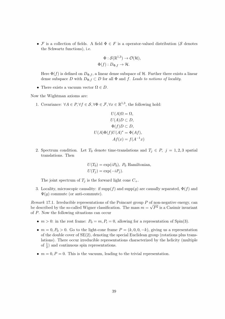
• F is a collection of fields. A field Φ ∈ F is a operator-valued distribution (S denotesthe Schwartz functions), i.e.

Φ : S(R1,3)→ O(H),

Φ(f) : DΦ,f → H.

Here Φ(f) is defined on DΦ,f , a linear dense subspace of H. Further there exists a lineardense subspace D with DΦ,f ⊂ D for all Φ and f . Leads to notions of locality.

• There exists a vacuum vector Ω ∈ D.

Now the Wightman axioms are:

1. Covariance: ∀A ∈ P,∀f ∈ S, ∀Φ ∈ F ,∀x ∈ R1,3, the following hold:

U(A)Ω = Ω,

U(A)D ⊂ D,Φ(f)D ⊂ D,

U(A)Φ(f)U(A)∗ = Φ(Af),

Af(x) = f(A−1x)

2. Spectrum condition. Let T0 denote time-translations and Tj ∈ P, j = 1, 2, 3 spatialtranslations. Then

U(T0) = exp(iP0), P0 Hamiltonian,U(Tj) = exp(−iPj).

The joint spectrum of Tj is the forward light cone C+.

3. Locality, microscopic causality: if supp(f) and supp(g) are causally separated, Φ(f) andΨ(g) commute (or anti-commute).

Remark 17.1. Irreducible representations of the Poincaré group P of non-negative energy, canbe described by the so-called Wigner classification. The mass m =

√P 2 is a Casimir invariant

of P . Now the following situations can occur

• m > 0: in the rest frame: P0 = m,Pi = 0, allowing for a representation of Spin(3).

• m = 0, P0 > 0. Go to the light-cone frame P = (k, 0, 0,−k), giving us a representationof the double cover of SE(2), denoting the special Euclidean group (rotations plus trans-lations). There occur irreducible representations characterized by the helicity (multipleof 1

2) and continuous spin representations.

• m = 0, P = 0. This is the vacuum, leading to the trivial representation.

39

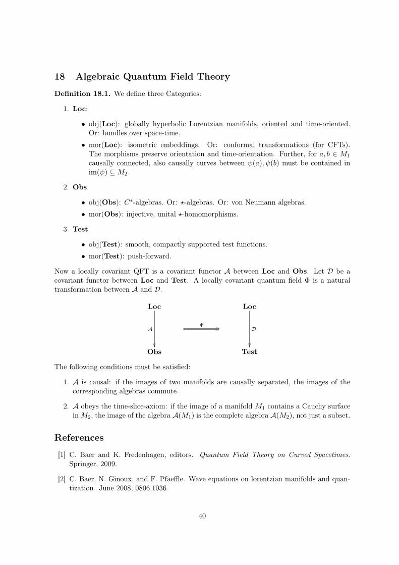
18 Algebraic Quantum Field Theory

Definition 18.1. We define three Categories:

1. Loc:

• obj(Loc): globally hyperbolic Lorentzian manifolds, oriented and time-oriented.Or: bundles over space-time.

• mor(Loc): isometric embeddings. Or: conformal transformations (for CFTs).The morphisms preserve orientation and time-orientation. Further, for a, b ∈ M1

causally connected, also causally curves between ψ(a), ψ(b) must be contained inim(ψ) ⊆M2.

2. Obs

• obj(Obs): C∗-algebras. Or: ?-algebras. Or: von Neumann algebras.

• mor(Obs): injective, unital ?-homomorphisms.

3. Test

• obj(Test): smooth, compactly supported test functions.

• mor(Test): push-forward.

Now a locally covariant QFT is a covariant functor A between Loc and Obs. Let D be acovariant functor between Loc and Test. A locally covariant quantum field Φ is a naturaltransformation between A and D.

Loc

A

Loc

D

Φ +3

Obs Test

The following conditions must be satisfied:

1. A is causal: if the images of two manifolds are causally separated, the images of thecorresponding algebras commute.

2. A obeys the time-slice-axiom: if the image of a manifold M1 contains a Cauchy surfaceinM2, the image of the algebra A(M1) is the complete algebra A(M2), not just a subset.

References

[1] C. Baer and K. Fredenhagen, editors. Quantum Field Theory on Curved Spacetimes.Springer, 2009.

[2] C. Baer, N. Ginoux, and F. Pfaeffle. Wave equations on lorentzian manifolds and quan-tization. June 2008, 0806.1036.

40

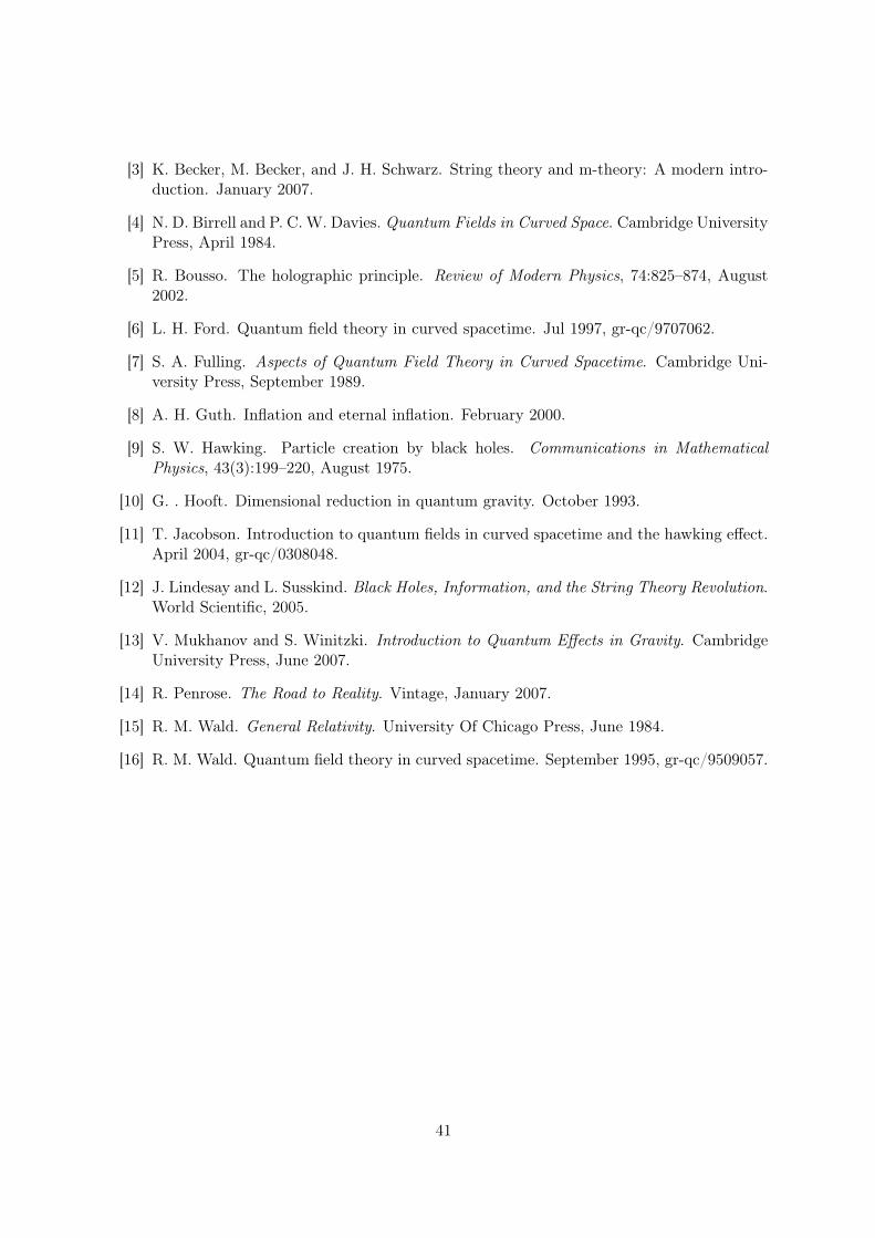
[3] K. Becker, M. Becker, and J. H. Schwarz. String theory and m-theory: A modern intro-duction. January 2007.

[4] N. D. Birrell and P. C. W. Davies. Quantum Fields in Curved Space. Cambridge UniversityPress, April 1984.

[5] R. Bousso. The holographic principle. Review of Modern Physics, 74:825–874, August2002.

[6] L. H. Ford. Quantum field theory in curved spacetime. Jul 1997, gr-qc/9707062.

[7] S. A. Fulling. Aspects of Quantum Field Theory in Curved Spacetime. Cambridge Uni-versity Press, September 1989.

[8] A. H. Guth. Inflation and eternal inflation. February 2000.

[9] S. W. Hawking. Particle creation by black holes. Communications in MathematicalPhysics, 43(3):199–220, August 1975.

[10] G. . Hooft. Dimensional reduction in quantum gravity. October 1993.

[11] T. Jacobson. Introduction to quantum fields in curved spacetime and the hawking effect.April 2004, gr-qc/0308048.

[12] J. Lindesay and L. Susskind. Black Holes, Information, and the String Theory Revolution.World Scientific, 2005.

[13] V. Mukhanov and S. Winitzki. Introduction to Quantum Effects in Gravity. CambridgeUniversity Press, June 2007.

[14] R. Penrose. The Road to Reality. Vintage, January 2007.

[15] R. M. Wald. General Relativity. University Of Chicago Press, June 1984.

[16] R. M. Wald. Quantum field theory in curved spacetime. September 1995, gr-qc/9509057.

41