Space and time in quantum cosmology

Space and time in quantum cosmology

Martin Bojowald

Institute for Gravitation and the Cosmos

The Pennsylvania State University

Space-time – p. 1

Space and time in quantum gravity

General relativity determines dynamics and structure ofspace-time.

1. Background independence.

Space-time structure may be non-classical.

It may happen that no consistent quantum space-time structureexists, not even semiclassically.

2. Problem of time.

Time transformations and evolution.

Space-time – p. 2

Hamiltonian constraint

Friedmann equation implies constraint

C = −6πGV p2V + V ρmatter = 0

for “volume” V = a3 and its momentum pV in isotropic models.

→ How is evolution derived from Wheeler–DeWitt equationafter quantization, replacing pV ∝ a with −i~∂/∂V ?

→ Can quantum corrections in C be consistent with largeralgebra including diffeomorphism constraint?

Is there a consistent space-time line element

ds2 = −dτ2 + a(τ)2(dx2 + dy2 + dz2)

where a solves a quantum corrected Friedmann equation?

Space-time – p. 3

Examples in loop quantum gravity

1. Dressed-metric approach for cosmological inhomogeneity.[Agulló, Ashtekar, Nelson: PRL 109 (2012) 251301]

2. Partial Abelianization of spherically symmetric models.[Gambini, Pullin: PRL 110 (2013) 211301]

3. “Transfiguration” of black holes.[Ashtekar, Olmedo, Singh: PRL 121 (2018) 241301]

4. “Covariant polymerization” in spherically symmetric models.[Benítez, Gambini, Pullin: arXiv:2102.09501]

Attempted justification of model of critical collapse.[Benítez, Gambini, Lehner, Liebling, Pullin: PRL 124 (2020) 071301]

None of these claims are based on consistent space-timestructures.

Space-time – p. 4

Models of loop quantum gravity

Hamiltonian constraint quantized, but also modified:

Cmod = −6πGV f(pV )2 + V ρmatter = 0

with bounded function f(pV ) (holonomy modification).

Solutions: Energy density ρmatter ∝ f(pV )2 bounded.

May avoid singularities and suggest new physical effects.

Open questions:

→ Interplay between modification and other quantumcorrections, such as fluctuations?

→ Consistency with covariance conditions?Modification by f(pV ) not of standard higher-curvature form.

→ Special way to deal with problem of time(deparameterization) may be restrictive.

Space-time – p. 5

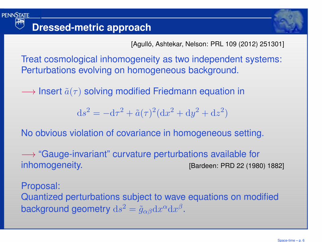
Dressed-metric approach

[Agulló, Ashtekar, Nelson: PRL 109 (2012) 251301]

Treat cosmological inhomogeneity as two independent systems:Perturbations evolving on homogeneous background.

−→ Insert a(τ) solving modified Friedmann equation in

ds2 = −dτ2 + a(τ)2(dx2 + dy2 + dz2)

No obvious violation of covariance in homogeneous setting.

−→ “Gauge-invariant” curvature perturbations available forinhomogeneity. [Bardeen: PRD 22 (1980) 1882]

Proposal:Quantized perturbations subject to wave equations on modified

background geometry ds2 = gαβdxαdxβ.

Space-time – p. 6

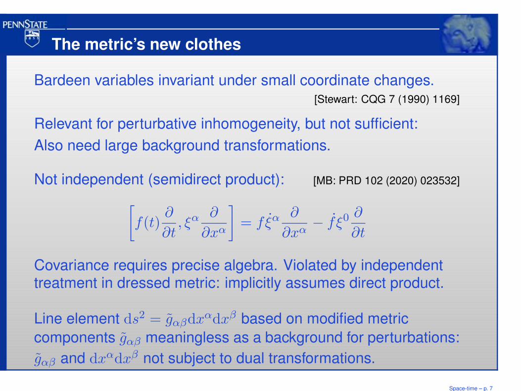
The metric’s new clothes

Bardeen variables invariant under small coordinate changes.[Stewart: CQG 7 (1990) 1169]

Relevant for perturbative inhomogeneity, but not sufficient:

Also need large background transformations.

Not independent (semidirect product): [MB: PRD 102 (2020) 023532]

[

f(t)∂

∂t, ξα

∂

∂xα

]

= fξα∂

∂xα− f ξ0

∂

∂t

Covariance requires precise algebra. Violated by independenttreatment in dressed metric: implicitly assumes direct product.

Line element ds2 = gαβdxαdxβ based on modified metric

components gαβ meaningless as a background for perturbations:

gαβ and dxαdxβ not subject to dual transformations.

Space-time – p. 7

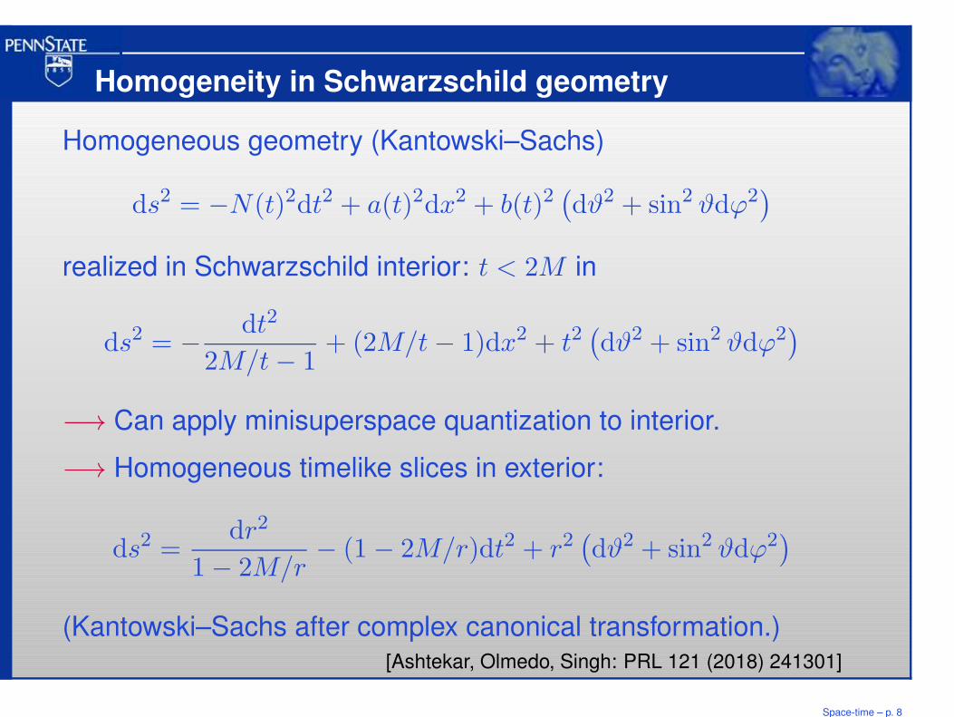
Homogeneity in Schwarzschild geometry

Homogeneous geometry (Kantowski–Sachs)

ds2 = −N(t)2dt2 + a(t)2dx2 + b(t)2(

dϑ2 + sin2 ϑdϕ2)

realized in Schwarzschild interior: t < 2M in

ds2 = −dt2

2M/t− 1+ (2M/t− 1)dx2 + t2

(

dϑ2 + sin2 ϑdϕ2)

−→ Can apply minisuperspace quantization to interior.

−→ Homogeneous timelike slices in exterior:

ds2 =dr2

1− 2M/r− (1− 2M/r)dt2 + r2

(

dϑ2 + sin2 ϑdϕ2)

(Kantowski–Sachs after complex canonical transformation.)[Ashtekar, Olmedo, Singh: PRL 121 (2018) 241301]

Space-time – p. 8

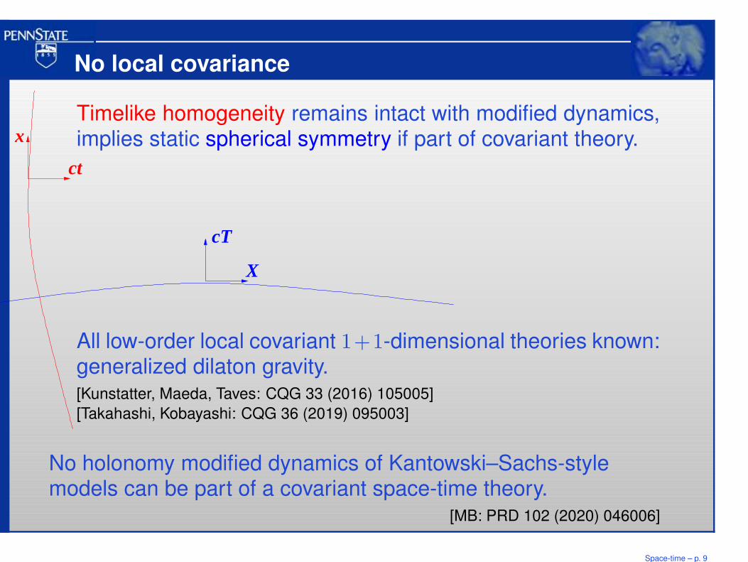
No local covariance

ct

x

X

cT

Timelike homogeneity remains intact with modified dynamics,implies static spherical symmetry if part of covariant theory.

All low-order local covariant 1+1-dimensional theories known:generalized dilaton gravity.[Kunstatter, Maeda, Taves: CQG 33 (2016) 105005]

[Takahashi, Kobayashi: CQG 36 (2019) 095003]

No holonomy modified dynamics of Kantowski–Sachs-stylemodels can be part of a covariant space-time theory.

[MB: PRD 102 (2020) 046006]

Space-time – p. 9

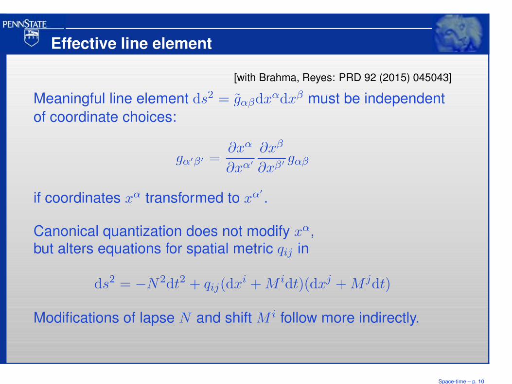
Effective line element

[with Brahma, Reyes: PRD 92 (2015) 045043]

Meaningful line element ds2 = gαβdxαdxβ must be independent

of coordinate choices:

gα′β′ =∂xα

∂xα′

∂xβ

∂xβ′gαβ

if coordinates xα transformed to xα′

.

Canonical quantization does not modify xα,but alters equations for spatial metric qij in

ds2 = −N2dt2 + qij(dxi +M idt)(dxj +M jdt)

Modifications of lapse N and shift M i follow more indirectly.

Space-time – p. 10

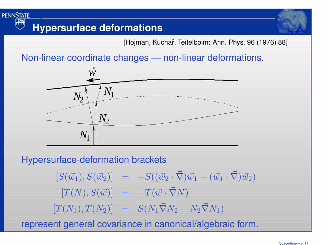
Hypersurface deformations

[Hojman, Kuchar, Teitelboim: Ann. Phys. 96 (1976) 88]

Non-linear coordinate changes — non-linear deformations.

N1

w

N2

N2

N1

Hypersurface-deformation brackets

[S(~w1), S(~w2)] = −S((~w2 · ~∇)~w1 − (~w1 · ~∇)~w2)

[T (N), S(~w)] = −T (~w · ~∇N)

[T (N1), T (N2)] = S(N1~∇N2 −N2

~∇N1)

represent general covariance in canonical/algebraic form.


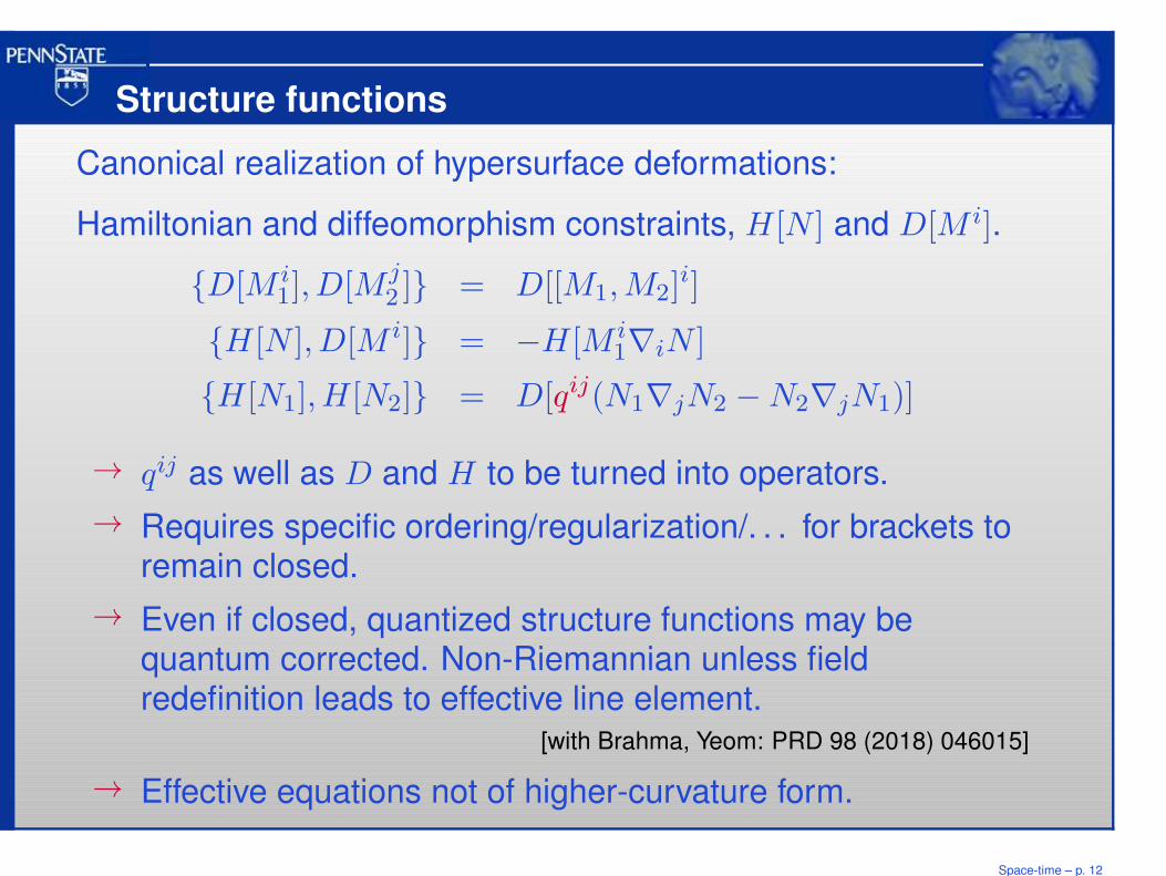
Structure functions

Canonical realization of hypersurface deformations:

Hamiltonian and diffeomorphism constraints, H[N ] and D[M i].

{D[M i1],D[M j

2 ]} = D[[M1,M2]i]

{H[N ],D[M i]} = −H[M i1∇iN ]

{H[N1],H[N2]} = D[qij(N1∇jN2 −N2∇jN1)]

→ qij as well as D and H to be turned into operators.

→ Requires specific ordering/regularization/. . . for brackets toremain closed.

→ Even if closed, quantized structure functions may bequantum corrected. Non-Riemannian unless fieldredefinition leads to effective line element.

[with Brahma, Yeom: PRD 98 (2018) 046015]

→ Effective equations not of higher-curvature form.


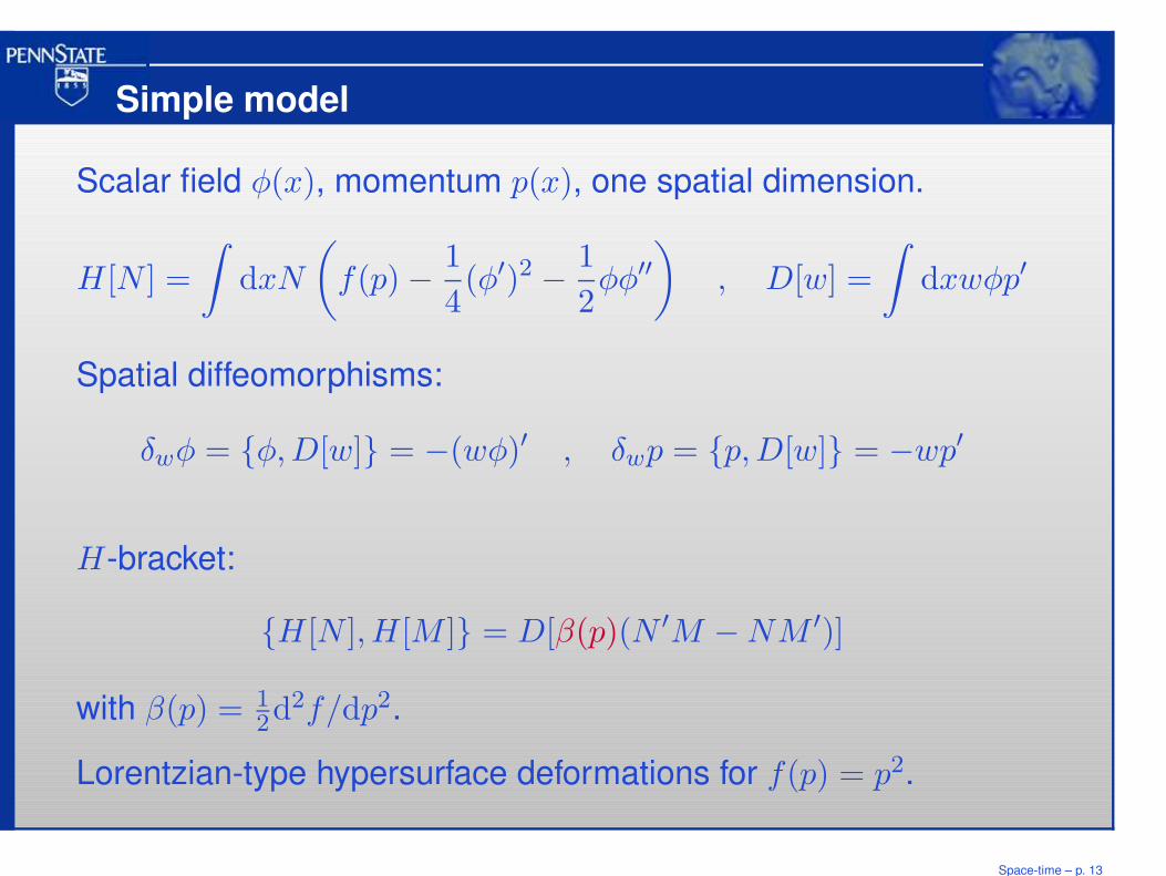
Simple model

Scalar field φ(x), momentum p(x), one spatial dimension.

H[N ] =

∫

dxN

(

f(p)−1

4(φ′)2 −

1

2φφ′′

)

, D[w] =

∫

dxwφp′

Spatial diffeomorphisms:

δwφ = {φ,D[w]} = −(wφ)′ , δwp = {p,D[w]} = −wp′

H-bracket:

{H[N ],H[M ]} = D[β(p)(N ′M −NM ′)]

with β(p) = 12d2f/dp2.

Lorentzian-type hypersurface deformations for f(p) = p2.


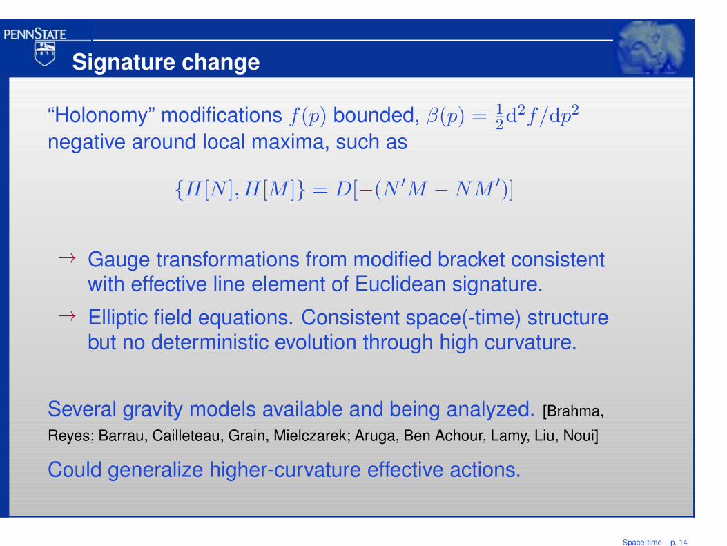
Signature change

“Holonomy” modifications f(p) bounded, β(p) = 12d2f/dp2

negative around local maxima, such as

{H[N ],H[M ]} = D[−(N ′M −NM ′)]

→ Gauge transformations from modified bracket consistentwith effective line element of Euclidean signature.

→ Elliptic field equations. Consistent space(-time) structurebut no deterministic evolution through high curvature.

Several gravity models available and being analyzed. [Brahma,

Reyes; Barrau, Cailleteau, Grain, Mielczarek; Aruga, Ben Achour, Lamy, Liu, Noui]

Could generalize higher-curvature effective actions.


Status of covariance in loop models

��

��

��

��

��

��

��

��

��

��

��

��

��

��

��

��

��

��

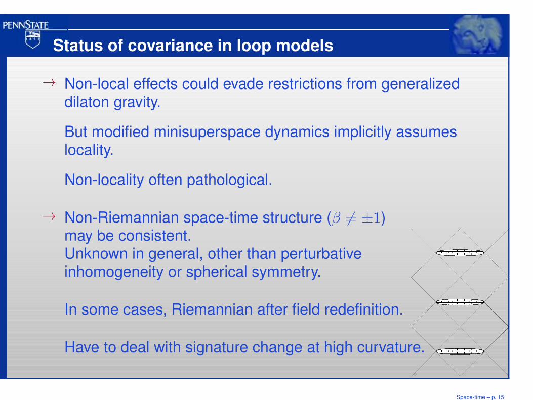
→ Non-local effects could evade restrictions from generalizeddilaton gravity.

But modified minisuperspace dynamics implicitly assumeslocality.

Non-locality often pathological.

→ Non-Riemannian space-time structure (β 6= ±1)may be consistent.Unknown in general, other than perturbativeinhomogeneity or spherical symmetry.

In some cases, Riemannian after field redefinition.

Have to deal with signature change at high curvature.


Problem of time

Friedmann constraint with scalar field φ, momentum pφ:

C =1

2

p2φV

+1

2V m2φ2 − 6πGV p2V

= (−pφ +H(V, pV , φ)) (pφ +H(V, pV , φ))

implies relational Hamiltonian

H(V, pV , φ) = ±√

12πGV 2(p2V −m2φ2)

for evolution of (V, pV ) with respect to φ.

Simplifies for popular case of m = 0 (deparameterization).

Not generic as fundamental field φ: no mass or self-interactions.

Unitarity if φ might run back and forth for m 6= 0?


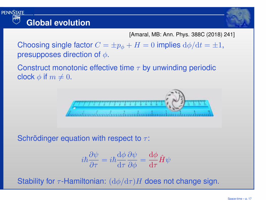
Global evolution

[Amaral, MB: Ann. Phys. 388C (2018) 241]

Choosing single factor C = ±pφ +H = 0 implies dφ/dt = ±1,

presupposes direction of φ.

Construct monotonic effective time τ by unwinding periodicclock φ if m 6= 0.

Schrödinger equation with respect to τ :

i~∂ψ

∂τ= i~

dφ

dτ

∂ψ

∂φ=

dφ

dτHψ

Stability for τ -Hamiltonian: (dφ/dτ)H does not change sign.


Unwinding time: C = −p2φ − λ2φ2 +H20

φ

τ

n=−1 n=0 n=1

→ Solve i~∂ψk/∂φ = ±√

E2k − λ2φ2ψk where H0ψk = Ekψk.

→ For given clock Hamiltonian, construct piecewise linear φ(τ)alternating between φ+(τ) = τ + A+ and φ−(τ) = −τ +A−.

→ Insert φ(τ) in φk(φ). Alternate signs for constant

sgn(dφ/dτ)H, where H = ±√

H20 − λ2φ2.

→ Obtain ψ(τ) as superposition of H0-stationary states ψk(τ)according to desired initial state.


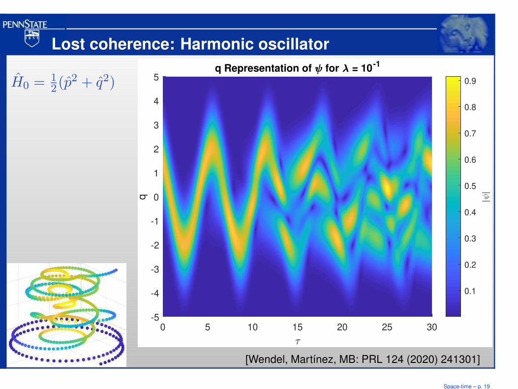
Lost coherence: Harmonic oscillator

0 5 10 15 20 25 30-5

-4

-3

-2

-1

0

1

2

3

4

5

q

q Representation of for = 10-1

0.1

0.2

0.3

0.4

0.5

0.6

0.7

0.8

0.9

||

H0 =12(p2 + q2)

[Wendel, Martínez, MB: PRL 124 (2020) 241301]


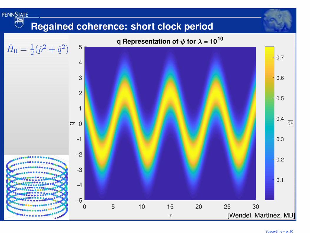
Regained coherence: short clock period

0 5 10 15 20 25 30-5

-4

-3

-2

-1

0

1

2

3

4

5

q

q Representation of for = 1010

0.1

0.2

0.3

0.4

0.5

0.6

0.7

||

H0 =12(p2 + q2)

[Wendel, Martínez, MB]


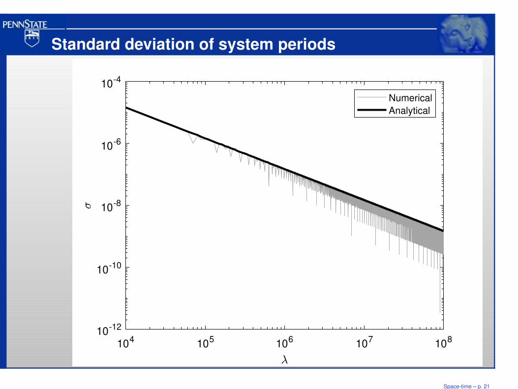
Standard deviation of system periods

104

105

106

107

108

10-12

10-10

10-8

10-6

10-4

Numerical

Analytical


Upper bound

TC ≈ 9.7σTS based on theory of fundamental clock.

If TS can be measured with accuracy σ, then TC cannot begreater than 9.7σTS.

Latest atomic clocks: σ ≈ 10−19 at system period of TS ≈ 2 fs.[Campbell et al. Science 358 (2017) 98]

Therefore,

TC < 2 · 10−33 s ≈ 0.5 · 1011tP

Smallest direct measurement: Photon travel time acrosshydrogen molecule, 247 · 10−21s. [Grundmann et al. Science 370 (2020) 339]

Particle accelerators probe spatial distances of 10−20m ≈ 1016ℓP.

Corresponds to ≈ 10−28 s.


Implications

→ Deparameterization (λ = 0) approximates an oscillatingclock as long as system period larger than clock period.

→ New effects when system scales are Planckian.

→ Background independence: Space-time structure to bederived. Inserting modified solutions in classical-type lineelements not always consistent.

→ Hypersurface deformations in space-time provide powerfulalgebraic means to analyze space-time without strongassumptions about geometry.

→ No-go results in models of loop quantum gravity:Do not require specific form of modifications,use only qualitative features related to discreteness.Largely independent of specific approach.


Space and time in quantum cosmology

Documents

Transcript of Space and time in quantum cosmology