Solving Poisson’s equation using discontinuous elementswith Comsol Multiphysics

Michael Neilan

Louisiana State University

Department of Mathematics

Center for Computation & Technology

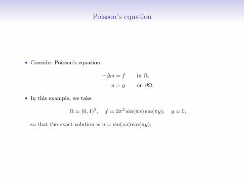
Poisson’s equation

• Consider Poisson’s equation:

−∆u = f in Ω,

u = g on ∂Ω.

• In this example, we take

Ω = (0, 1)2, f = 2π2 sin(πx) sin(πy), g = 0,

so that the exact solution is u = sin(πx) sin(πy).

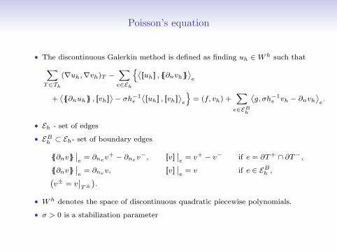
Poisson’s equation

• The discontinuous Galerkin method is defined as finding uh ∈Wh such thatXT∈Th

(∇uh,∇vh)T −X

e∈Eh

n˙[[uh]] , {{∂nvh}}

¸e

+˙{{∂nuh}} , [[vh]]

¸− σh−1e

˙[[uh]] , [[vh]]

¸e

o= (f, vh) +

Xe∈EB

h

˙g, σh−1e vh − ∂nvh

¸e.

• Eh - set of edges

• EBh ⊂ Eh- set of boundary edges

{{∂nv}}˛̨e

= ∂nev+ − ∂nev−, [[v]]

˛̨e

= v+ − v− if e = ∂T+ ∩ ∂T−,

{{∂nv}}˛̨e

= ∂nev, [[v]]˛̨e

= v if e ∈ EBh ,`v± = v

˛̨T±´.

• Wh denotes the space of discontinuous quadratic piecewise polynomials.

• σ > 0 is a stabilization parameter

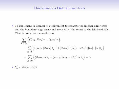
Discontinuous Galerkin methods

• To implement in Comsol it is convenient to separate the interior edge termsand the boundary edge terms and move all of the terms to the left-hand side.

That is, we write the method asXT∈Th

n(∇uh,∇vh)T − (f, vh)T

o−X

e∈EIh

n˙[[uh]] , {{∂nvh}}

¸e

+˙{{∂nuh}} , [[vh]]

¸− σh−1e

˙[[uh]] , [[vh]]

¸e

o−X

e∈EBh

n˙∂nuh, vh

¸e

+˙u− g, ∂nvh − σh−1e vh

¸e

o= 0.

• EIh - interior edges

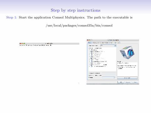
Step by step instructionsStep 1: Start the application Comsol Multiphysics. The path to the executable is

/usr/local/packages/comsol35a/bin/comsol

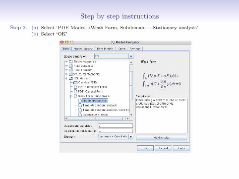
Step by step instructionsStep 2: (a) Select ‘PDE Modes→Weak Form, Subdomain→ Stationary analysis’

(b) Select ‘OK’

Step by step instructionsStep 3: (a) Select ‘Draw→Specific Object→Square’

(b) Select ‘OK’

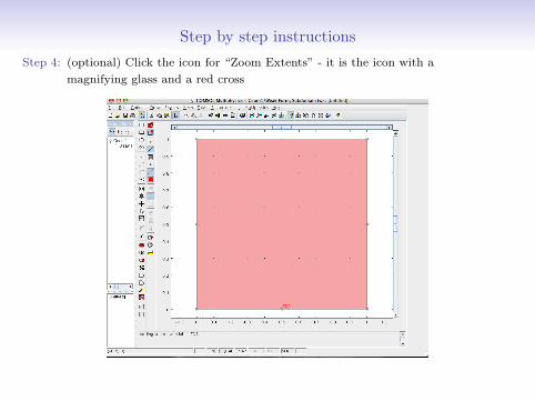
Step by step instructions

Step 4: (optional) Click the icon for “Zoom Extents” - it is the icon with a

magnifying glass and a red cross

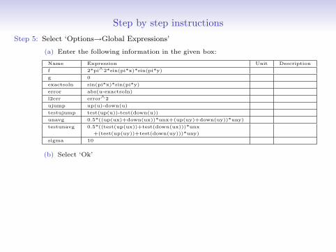
Step by step instructionsStep 5: Select ‘Options→Global Expressions’

(a) Enter the following information in the given box:

Name Expression Unit Description

f 2*pi∧2*sin(pi*x)*sin(pi*y)g 0

exactsoln sin(pi*x)*sin(pi*y)

error abs(u-exactsoln)

l2err error∧2ujump up(u)-down(u)

testujump test(up(u))-test(down(u))

unavg 0.5*((up(ux)+down(ux))*unx+(up(uy)+down(uy))*uny)

testunavg 0.5*((test(up(ux))+test(down(ux)))*unx+(test(up(uy))+test(down(uy)))*uny)

sigma 10

(b) Select ‘Ok’

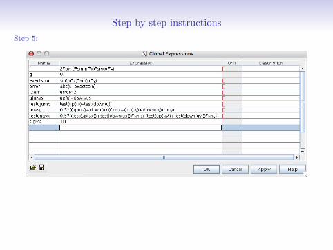
Step by step instructionsStep 5:

Step by step instructionsStep 6: (a) Select ‘Physics→Subdomain Settings’

(b) Enter the following information in each field:

weak : ux ∗ test(ux) + uy ∗ test(uy) − f ∗ test(u)

dweak : 0

bnd.weak : −unavg ∗ testujump − ujump ∗ testunavg + (sigma/h) ∗ ujump ∗ testujump

constr : 0

Constraint type : ideal

constrf : 0

(c) To use discontinuous elements, select the ‘Element tab’ and enter

‘shdisc(2,2,’u’)’ in the ‘shape’ field (the first 2 in ‘shdisc(2,2,’u’)’ is the

dimension, and the second 2 is the polynomial degree).

(d) Select ‘Ok’

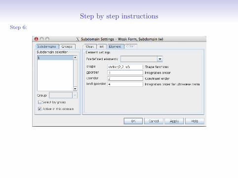
Step by step instructionsStep 6:

Step by step instructionsStep 7: (a) Select ‘Physics→Boundary Settings

(b) Under the “Weak” tab, select all four boundaries (1,2,3,4) and enter the

following information:

weak : −test(u) ∗ (ux ∗ nx + uy ∗ ny)− u ∗ (test(ux) ∗ nx + test(uy) ∗ ny)

+(sigma/h) ∗ u ∗ test(u)

dweak : 0

constr : 0

Constaint type : ideal

constrf : 0

(c) Select ‘OK’

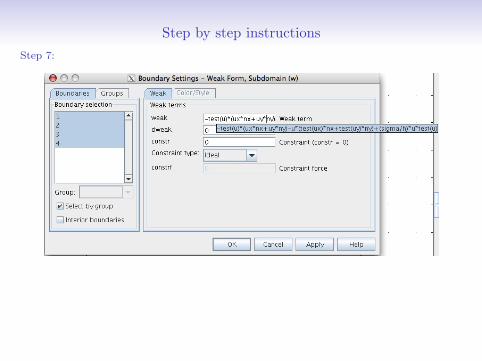
Step by step instructionsStep 7:

Step by step instructions

Step 8: Select the ‘Solve’ icon (the icon with a plain equal sign)

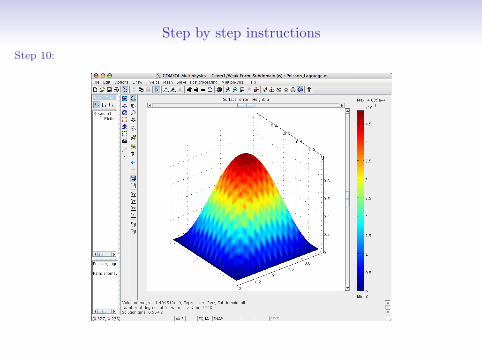
Step by step instructionsStep 9: To view the error,

(a) Select ’Post Processing→Plot Parameters’(b) Select the ’Surface tab’

(c) In the ’Surface Data Subtab’, enter ‘error’ in the Expression field

(d) Select the ’Height Data Subtab’ and check the box for Height Data

(e) Select ‘Apply’

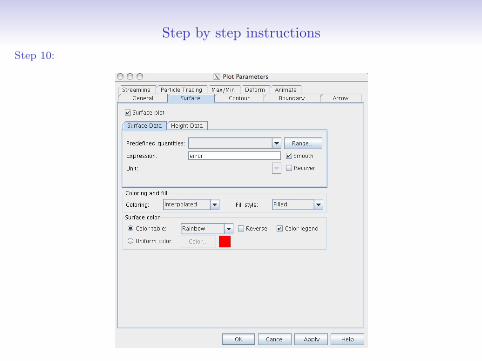
Step by step instructionsStep 10:

Step by step instructionsStep 10:

Step by step instructions

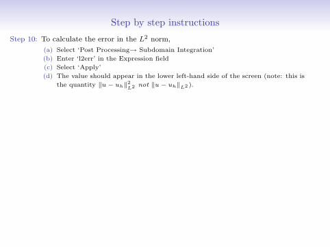
Step 10: To calculate the error in the L2 norm,

(a) Select ‘Post Processing→ Subdomain Integration’(b) Enter ‘l2err’ in the Expression field

(c) Select ‘Apply’

(d) The value should appear in the lower left-hand side of the screen (note: this is

the quantity ‖u− uh‖2L2 not ‖u− uh‖L2 ).