Analysis of Microsystems (AFM) 2010 - cpi.uni-freiburg.de
73
AFM
Transcript of Analysis of Microsystems (AFM) 2010 - cpi.uni-freiburg.de
AFM
OutlineScanning Probe Microscope (SPM)
•A family of microscopy forms where a sharp probe is scanned across a surface and some tip/sample interactions are monitored
•Scanning Tunneling Microscopy (STM)
•Atomic Force Microscopy (AFM)
contact mode
non-contact mode
tapping mode
•Other forms of SPM
lateral force
magnetic or electric force
thermal scanning
phase imaging
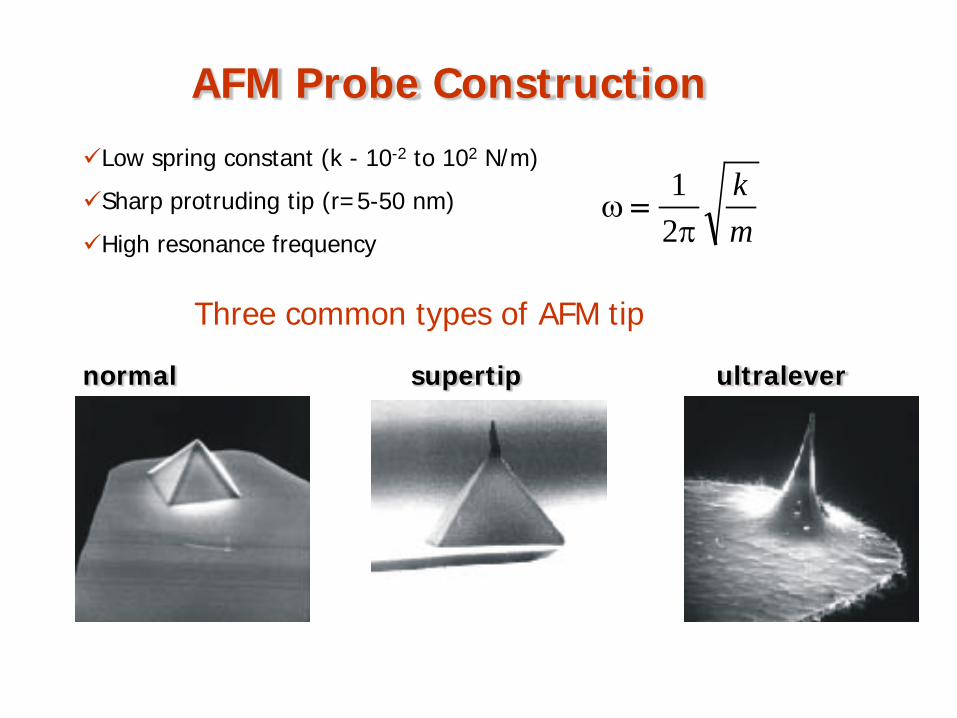
AFM Probe Construction
Low spring constant (k - 10-2 to 102 N/m)
Sharp protruding tip (r=5-50 nm)
High resonance frequency mk
πω
21
=
Three common types of AFM tip
normal supertip ultralever
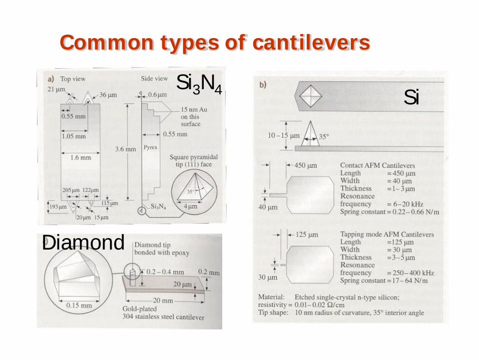
Common types of cantilevers
Si3N4 Si
Diamond
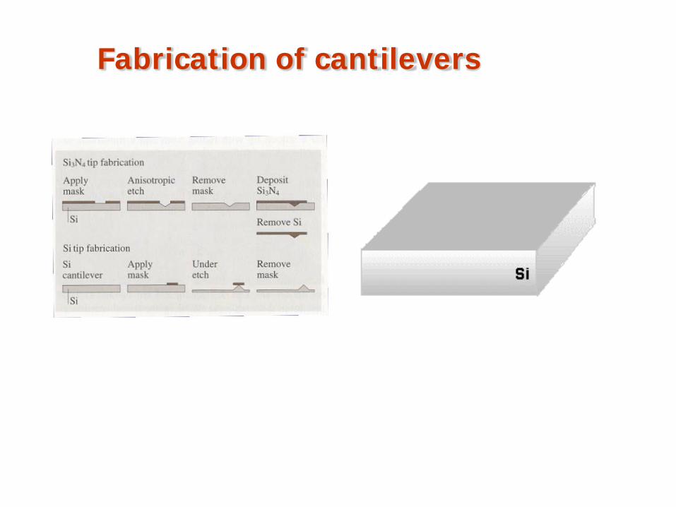
Fabrication of cantilevers
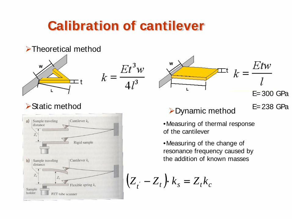
Calibration of cantilever
Theoretical method
Static methodDynamic method
•Measuring of thermal response of the cantilever
•Measuring of the change of resonance frequency caused by the addition of known masses
( ) ctstt kZkZZ ' =⋅−
E=300 GPa
E=238 GPa
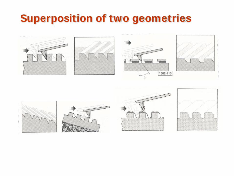
Superposition of two geometries
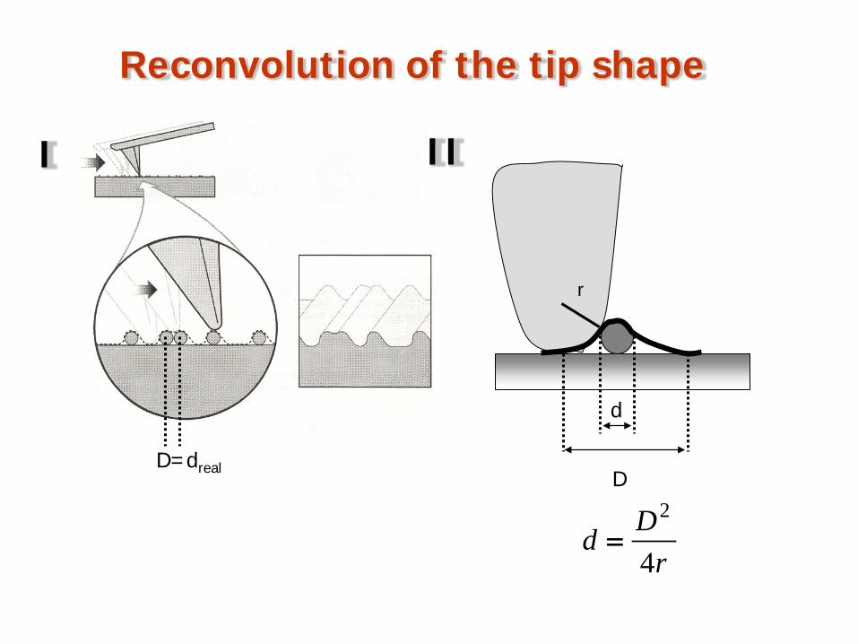
Reconvolution of the tip shape
D=dreal
r
d
D
I II
rDd4
2=
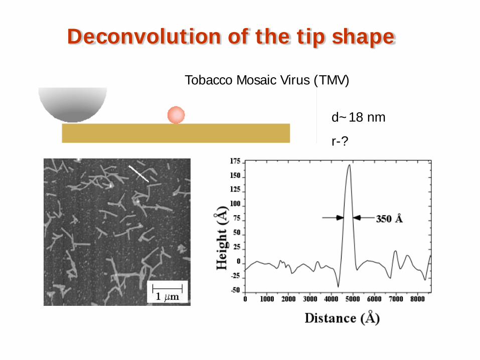
Deconvolution of the tip shape
Tobacco Mosaic Virus (TMV)
d~18 nm
r-?
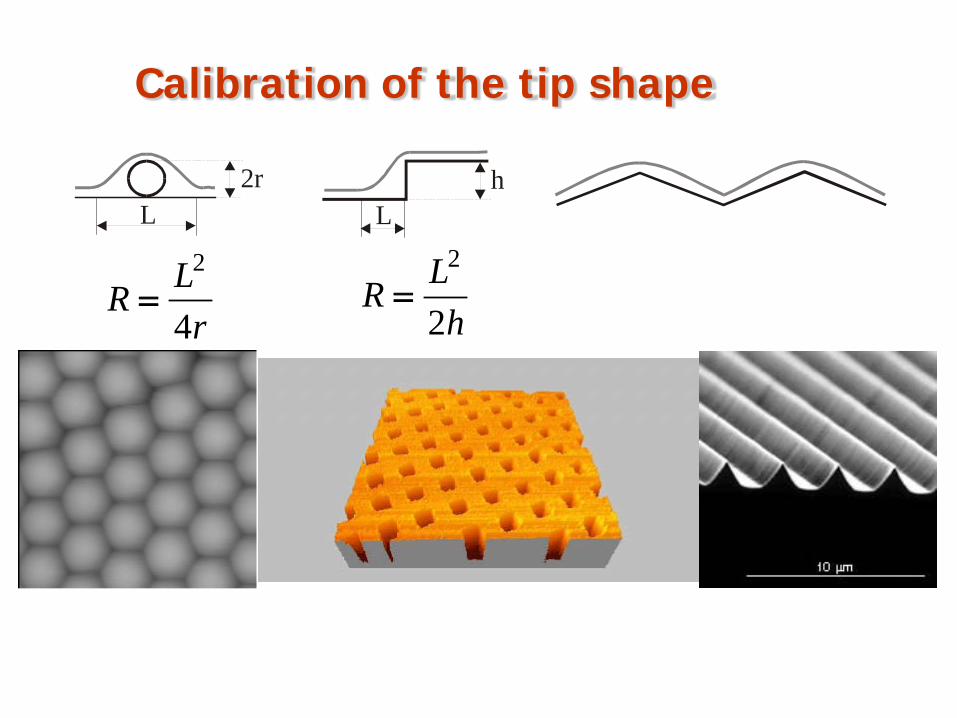
Calibration of the tip shape
hL
2rL
rLR4
2= h
LR2
2=
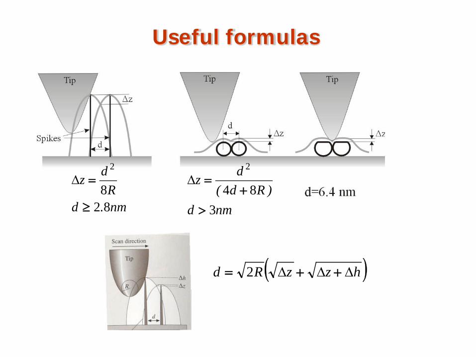
Useful formulas
nmd)Rd(
dz
384
2
>+
=∆
nm.dR
dz
828
2
≥
=∆
( )hzzRd ∆∆∆ ++= 2
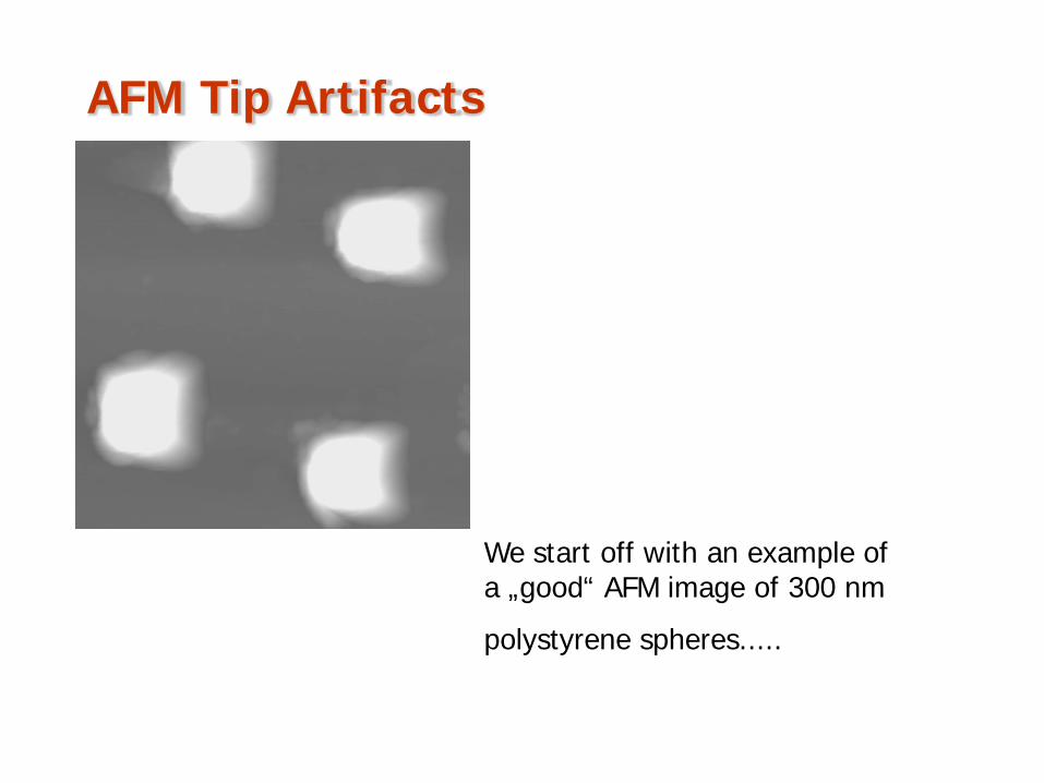
AFM Tip Artifacts
We start off with an example of a „good“ AFM image of 300 nm
polystyrene spheres.....
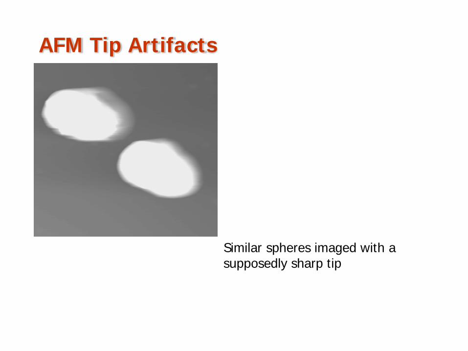
AFM Tip Artifacts
Similar spheres imaged with a supposedly sharp tip
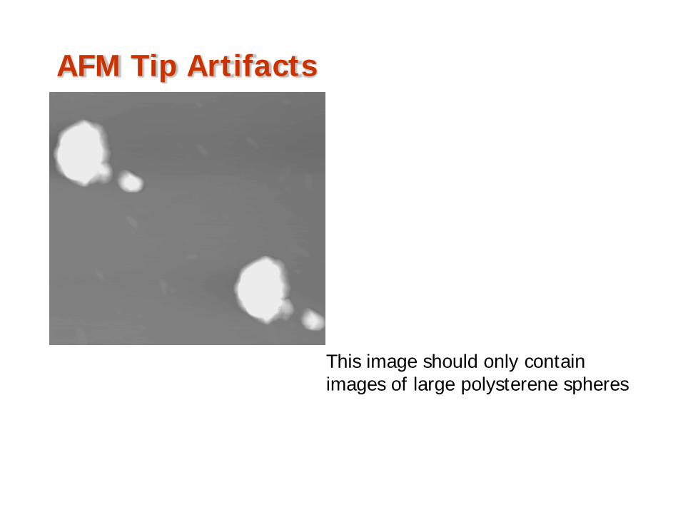
AFM Tip Artifacts
This image should only contain images of large polysterene spheres
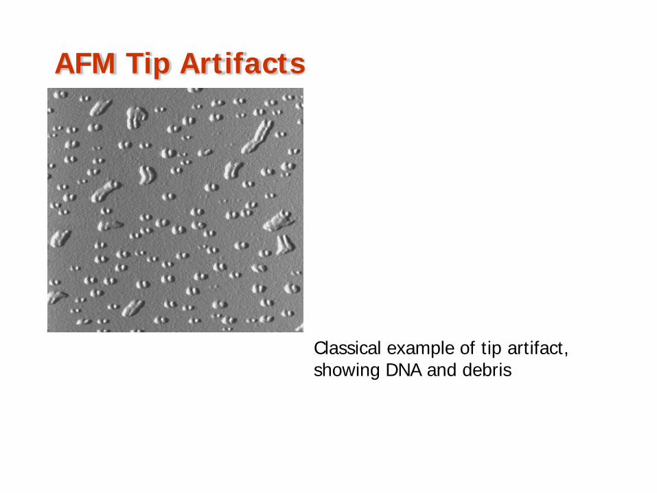
AFM Tip Artifacts
Classical example of tip artifact, showing DNA and debris
AFM Tip Artifacts
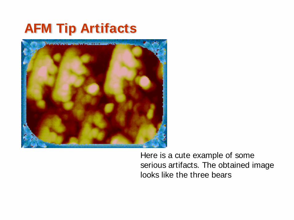
Here is a cute example of some serious artifacts. The obtained image looks like the three bears
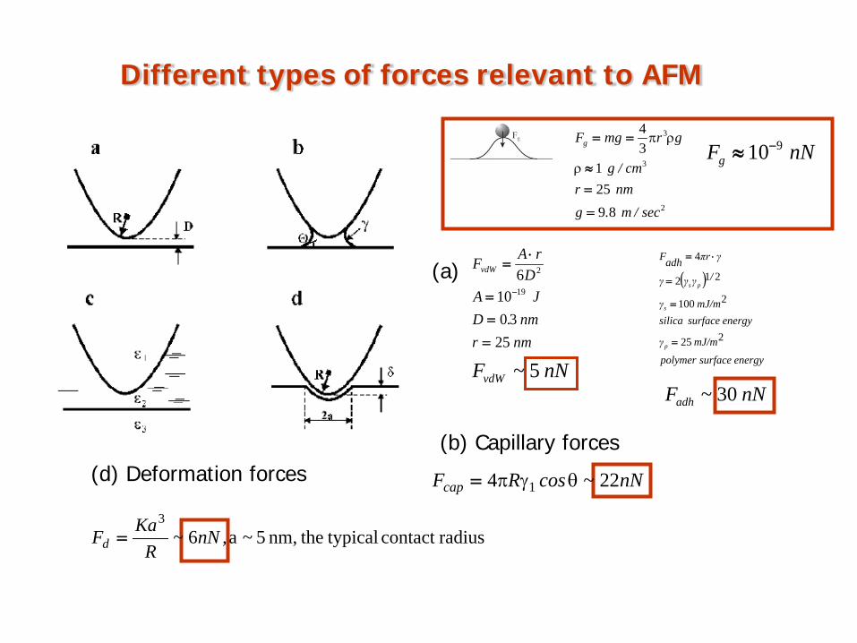
Different types of forces relevant to AFM
2
3
3
89251
34
sec/m.gnmr
cm/g
grmgFg
=
=≈
==
ρ
ρπ
nmrnm.D
JAD
rAFvdW
2530
10619
2
===
⋅=
−( )
energysurfacepolymermJ/mγ
energysurfacesilicamJ/mγ
/γγγ
γπradhF
p
s
ps
225
2100
212
4
=
=
=
⋅=
nNFg910−≈
nN~FvdW 5nN~Fadh 30
(b) Capillary forces
nN~cosRFcap 224 1 θγπ=(d) Deformation forces
radiuscontact typical thenm, 5 ~a 63
,nN~R
KaFd =
(a)
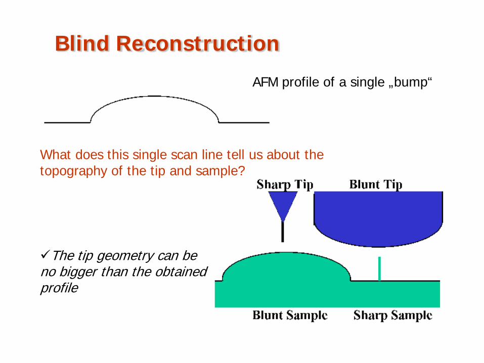
Blind Reconstruction
AFM profile of a single „bump“
What does this single scan line tell us about the topography of the tip and sample?
The tip geometry can be no bigger than the obtained profile
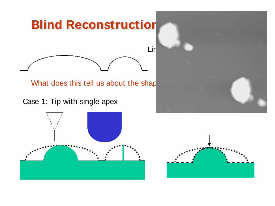
Blind Reconstruction
Line scan having two „bumps“
What does this tell us about the shape of the tip?
Case 1: Tip with single apex
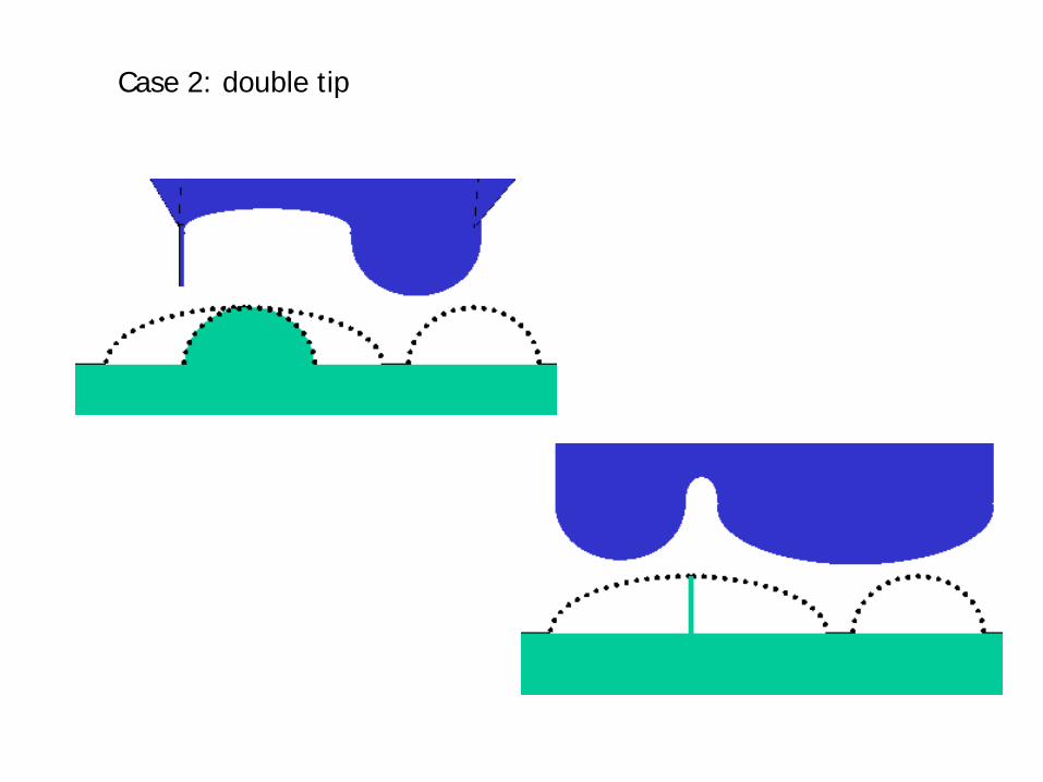
Case 2: double tip
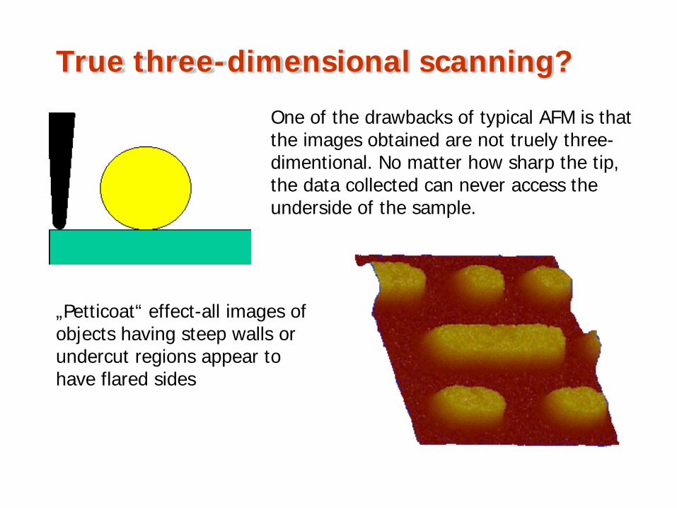
True three-dimensional scanning?
One of the drawbacks of typical AFM is that the images obtained are not truely three-dimentional. No matter how sharp the tip, the data collected can never access the underside of the sample.
„Petticoat“ effect-all images of objects having steep walls or undercut regions appear to have flared sides
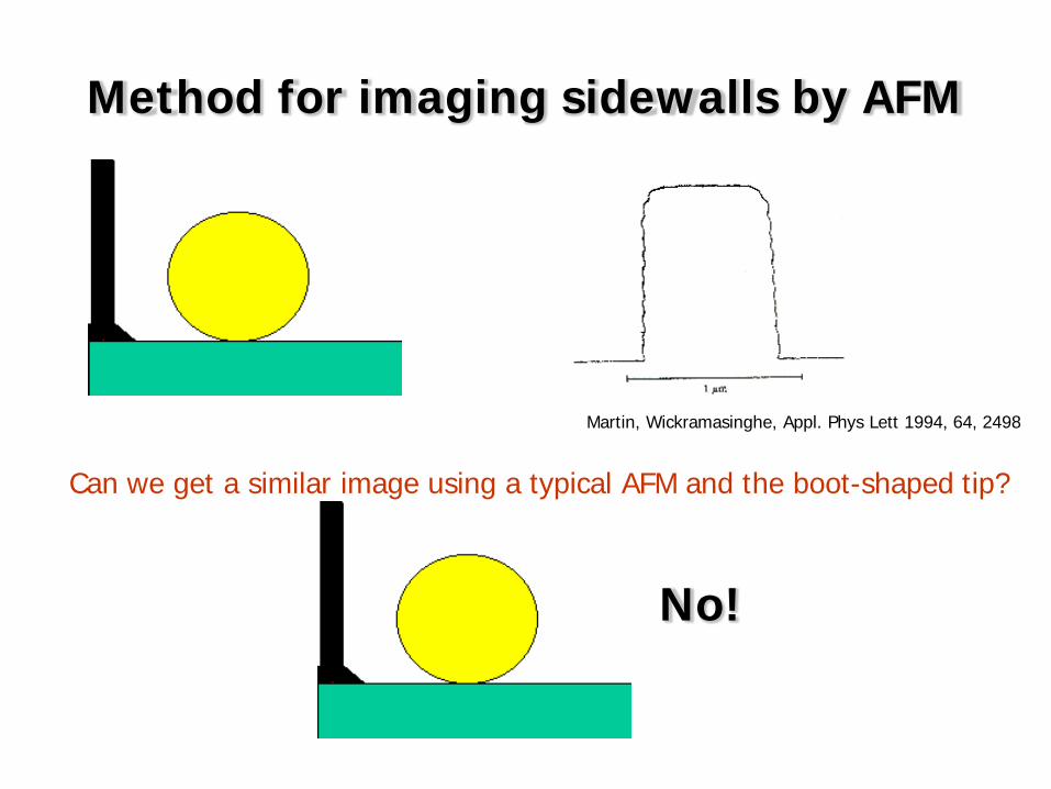
Method for imaging sidewalls by AFM
Martin, Wickramasinghe, Appl. Phys Lett 1994, 64, 2498
Can we get a similar image using a typical AFM and the boot-shaped tip?
No!
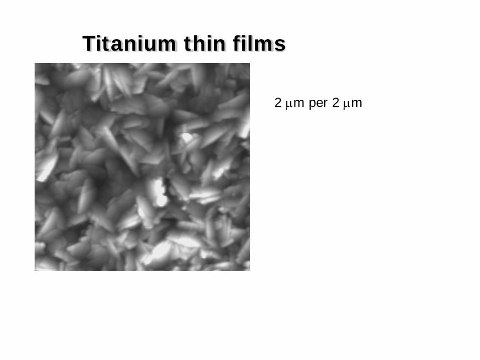
Titanium thin films
2 µm per 2 µm
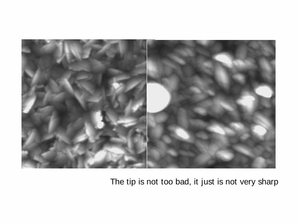
The tip is not too bad, it just is not very sharp
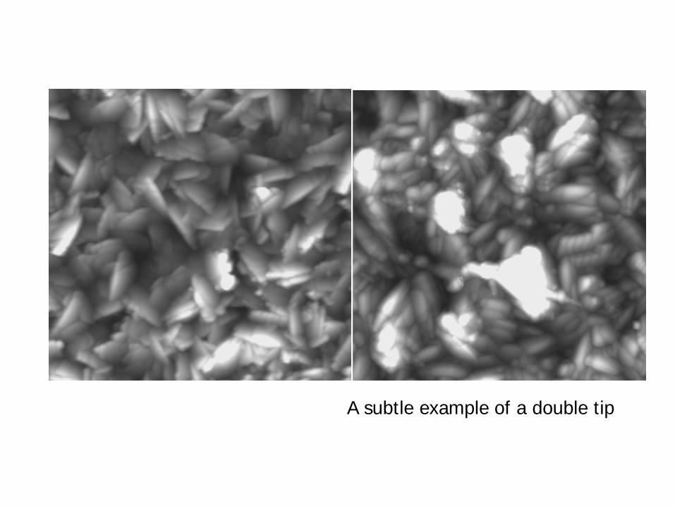
A subtle example of a double tip
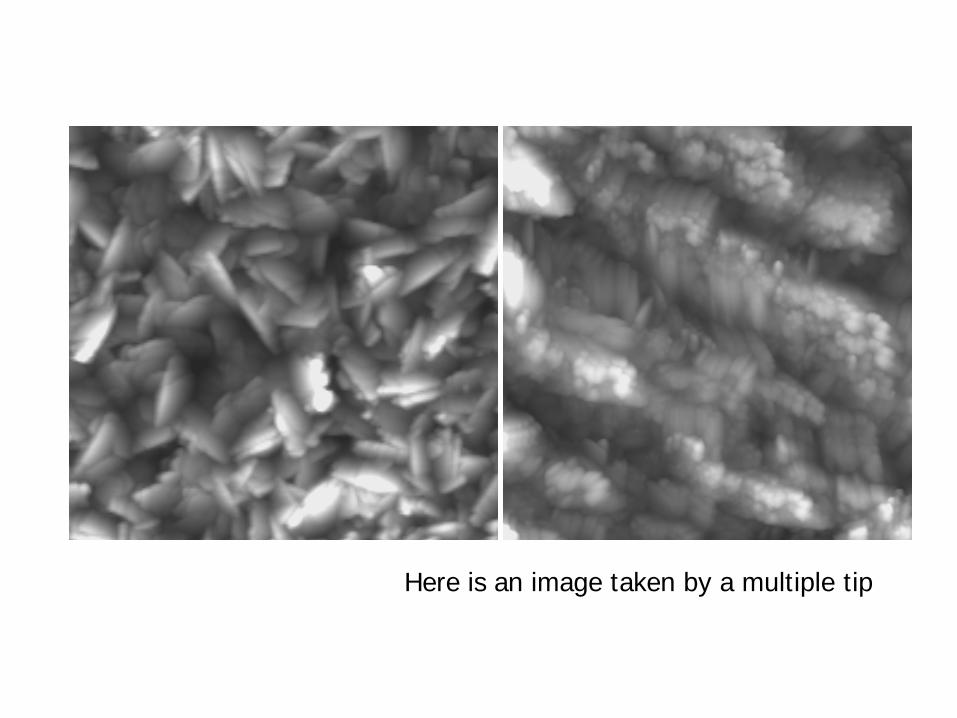
Here is an image taken by a multiple tip
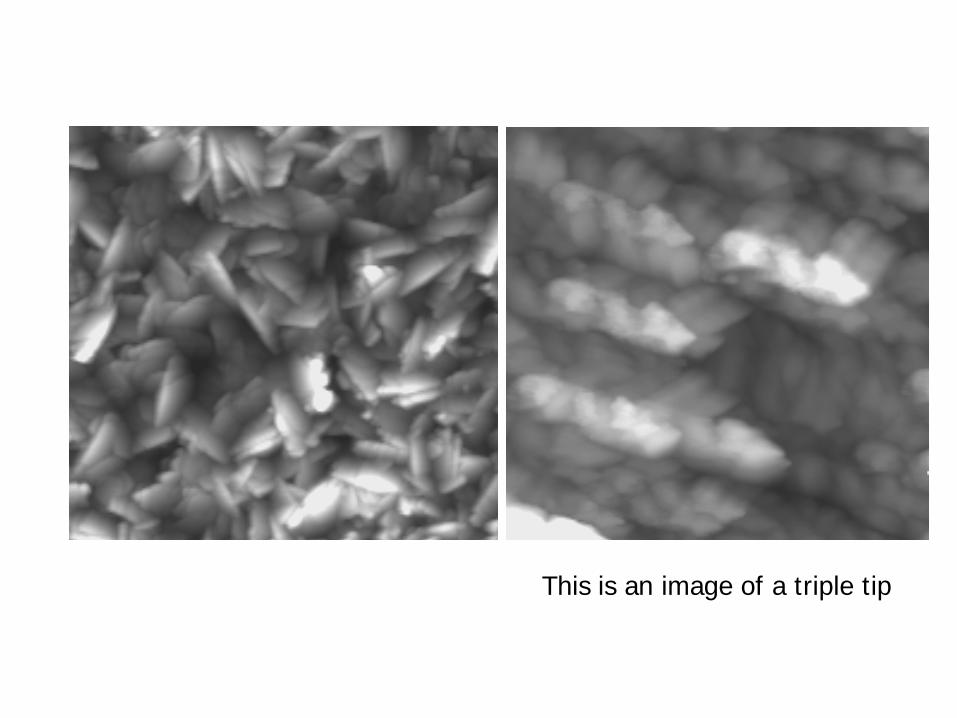
This is an image of a triple tip
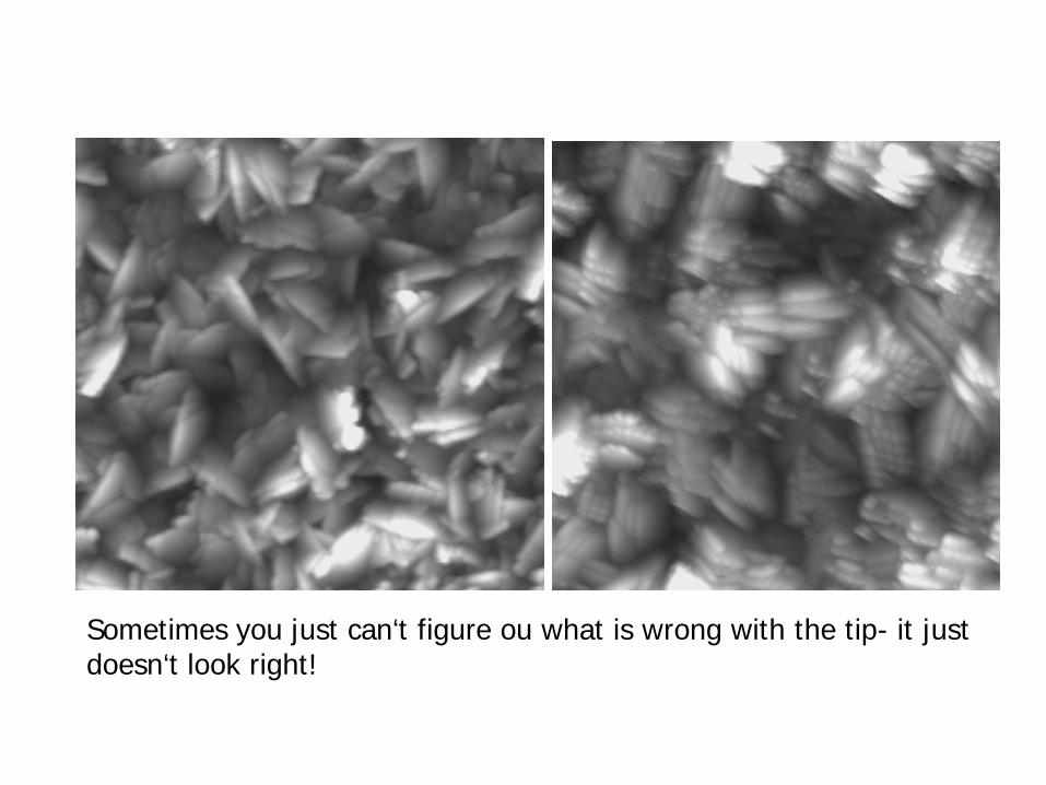
Sometimes you just can‘t figure ou what is wrong with the tip- it just doesn‘t look right!
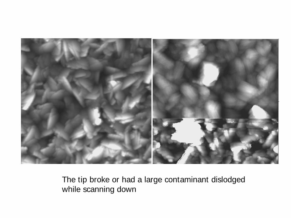
The tip broke or had a large contaminant dislodged while scanning down
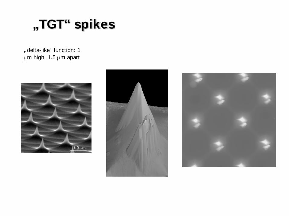
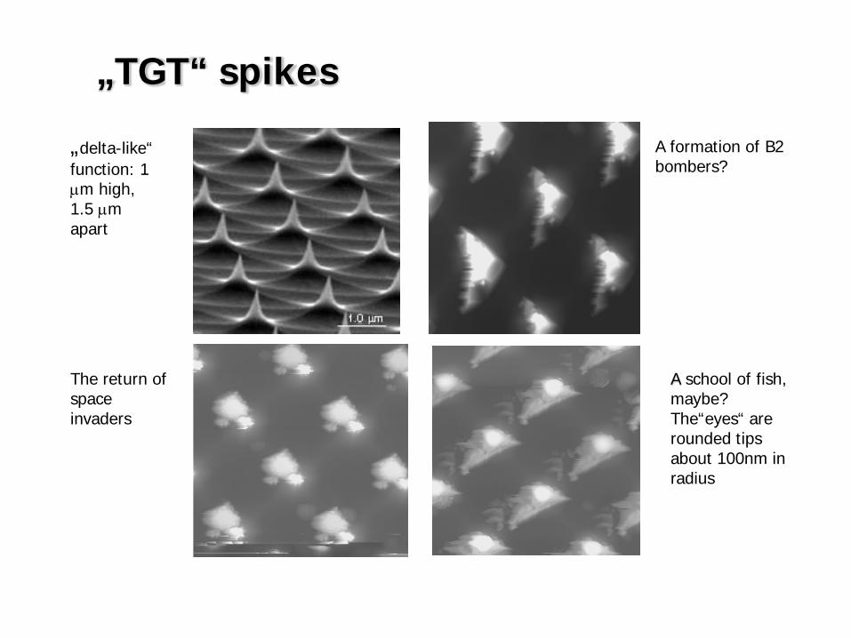
„TGT“ spikes
„delta-like“ function: 1 µm high, 1.5 µm apart
„TGT“ spikes
„delta-like“ function: 1 µm high, 1.5 µm apart
A school of fish, maybe? The“eyes“ are rounded tips about 100nm in radius
The return of space invaders
A formation of B2 bombers?
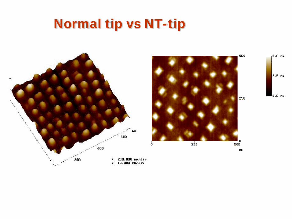
Normal tip vs NT-tip
Conclusion:
Golden rule of AFM spectroscopy:
Every time one measures one obtains an image
Not every time one obtains an artifact
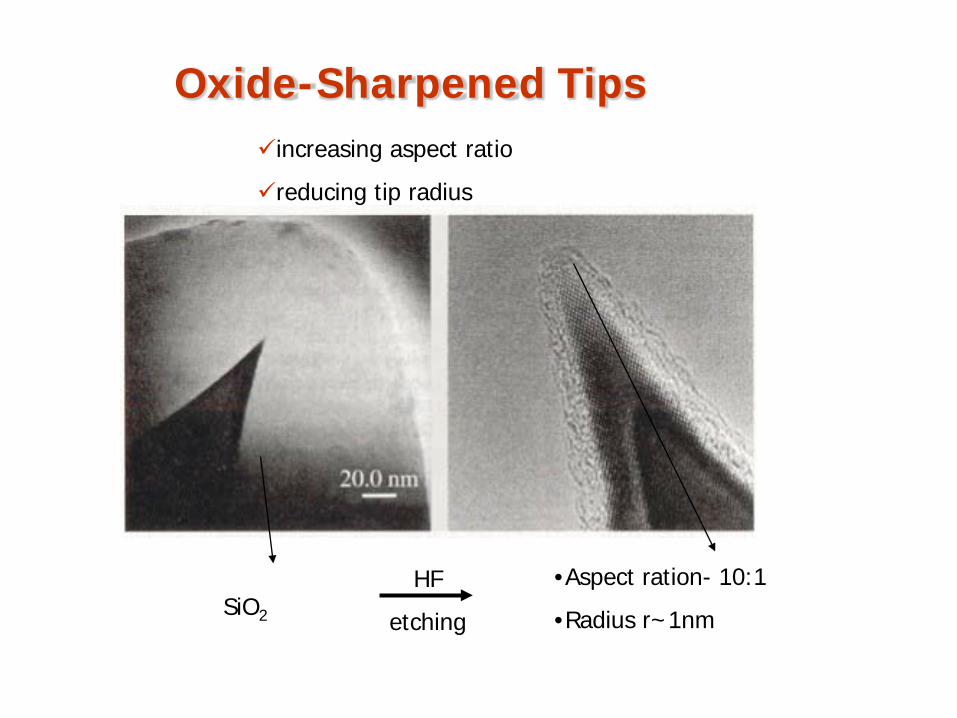
Oxide-Sharpened Tipsincreasing aspect ratio
reducing tip radius
•Aspect ration- 10:1
•Radius r~1nmSiO2
HF
etching
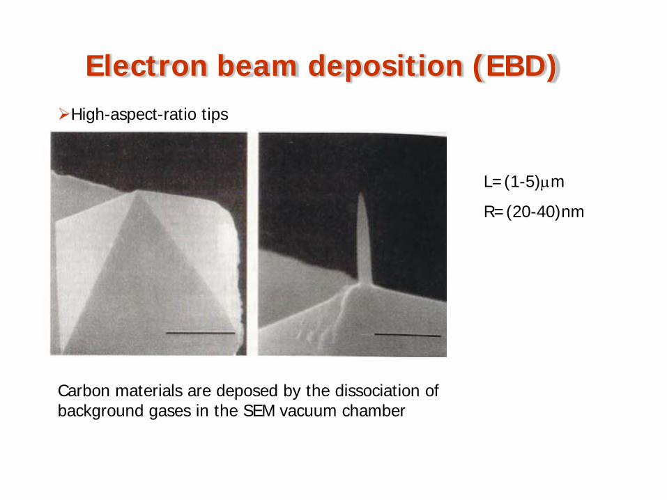
Electron beam deposition (EBD)High-aspect-ratio tips
Carbon materials are deposed by the dissociation of background gases in the SEM vacuum chamber
L=(1-5)µm
R=(20-40)nm
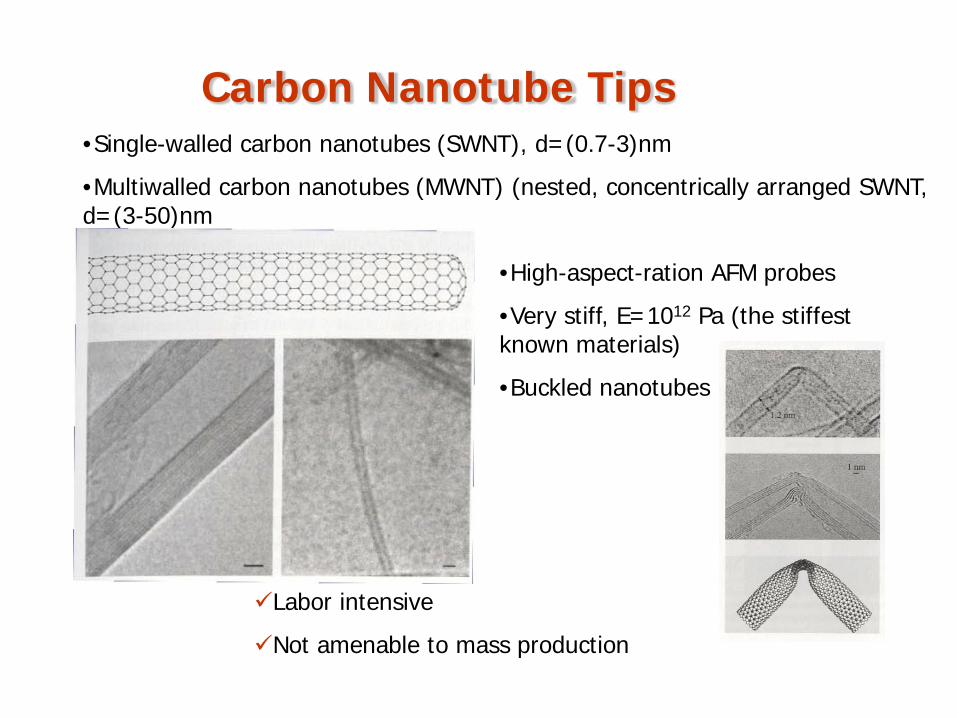
Carbon Nanotube Tips•Single-walled carbon nanotubes (SWNT), d=(0.7-3)nm
•Multiwalled carbon nanotubes (MWNT) (nested, concentrically arranged SWNT, d=(3-50)nm
•High-aspect-ration AFM probes
•Very stiff, E=1012 Pa (the stiffest known materials)
•Buckled nanotubes
Labor intensive
Not amenable to mass production
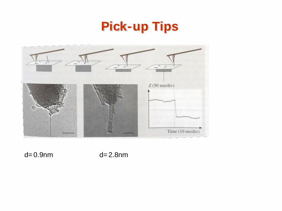
Pick-up Tips
d=0.9nm d=2.8nm
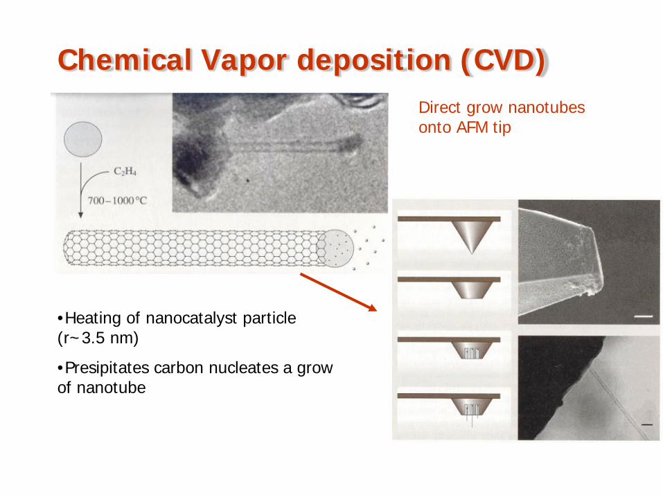
Chemical Vapor deposition (CVD)Direct grow nanotubes onto AFM tip
•Heating of nanocatalyst particle (r~3.5 nm)
•Presipitates carbon nucleates a grow of nanotube
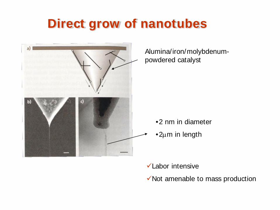
Direct grow of nanotubes
Alumina/iron/molybdenum-powdered catalyst
•2 nm in diameter
•2µm in length
Labor intensive
Not amenable to mass production
Modes of operation
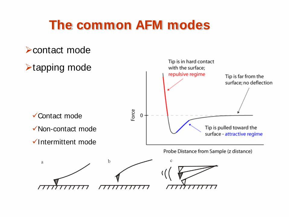
The common AFM modes
contact mode
tapping mode
Contact mode
Non-contact mode
Intermittent mode
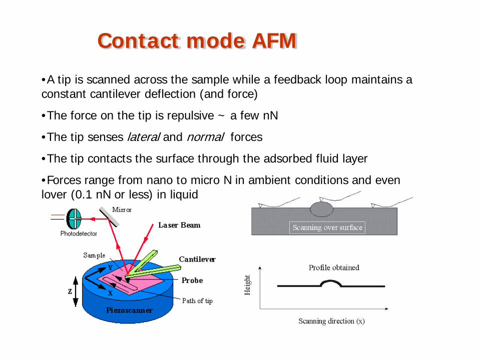
Contact mode AFM
•A tip is scanned across the sample while a feedback loop maintains a constant cantilever deflection (and force)
•The force on the tip is repulsive ~ a few nN
•The tip senses lateral and normal forces
•The tip contacts the surface through the adsorbed fluid layer
•Forces range from nano to micro N in ambient conditions and even lover (0.1 nN or less) in liquid
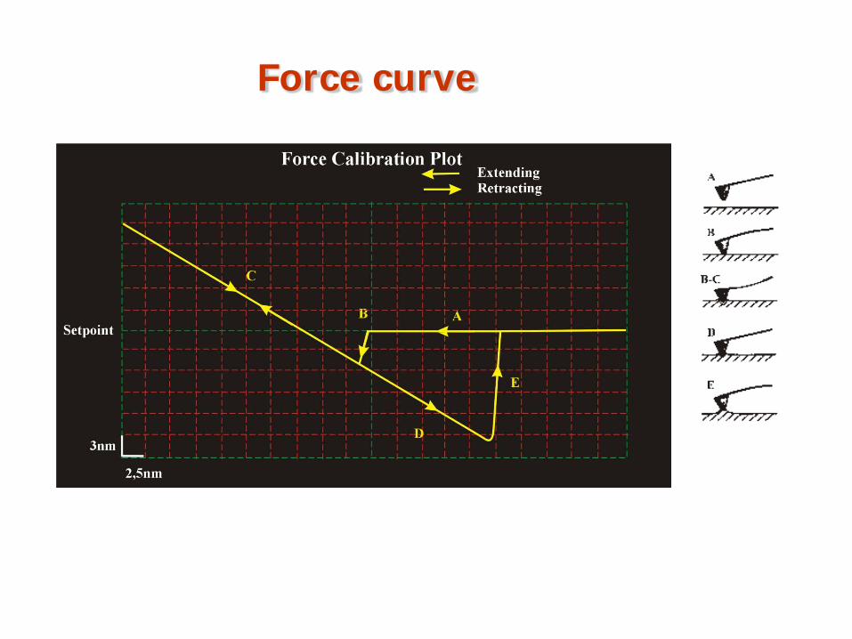
Force curve
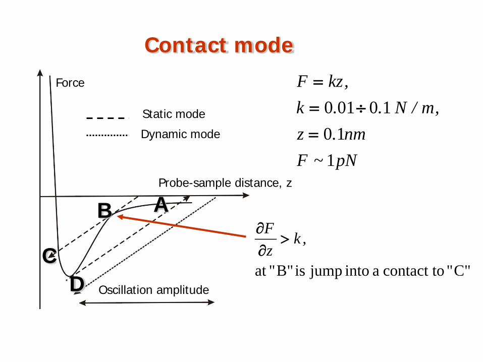
Contact mode
Force
Oscillation amplitude
Probe-sample distance, z
AB
CD
Static mode
Dynamic mode
pN~Fnm.z
,m/N..k,kzF
110
10010=
÷==
C"" contact to a into jump is B""at
,kzF>
∂∂
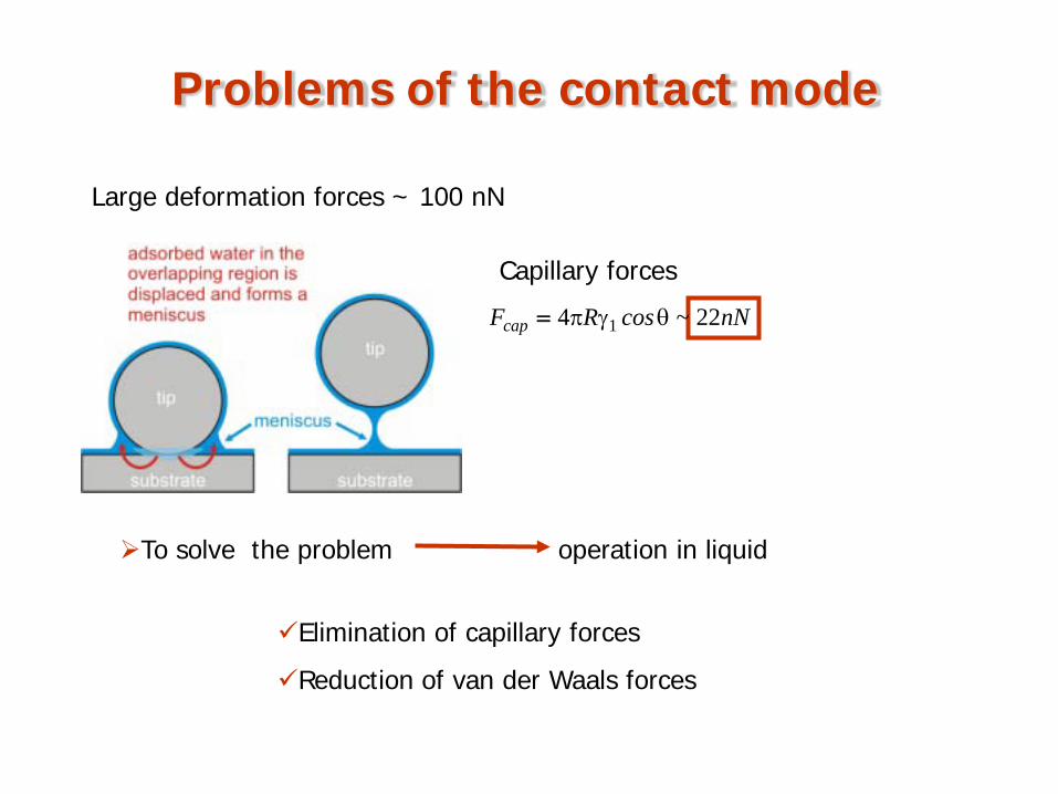
Problems of the contact mode
Large deformation forces ~ 100 nN
Capillary forces
nN~cosRFcap 224 1 θγπ=
To solve the problem operation in liquid
Elimination of capillary forces
Reduction of van der Waals forces
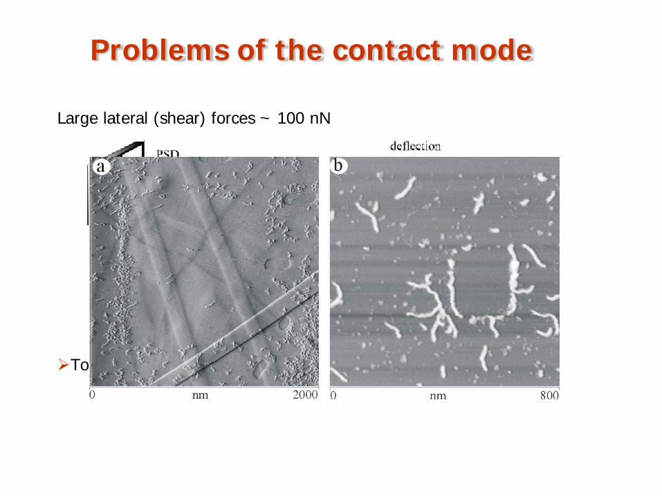
Problems of the contact mode
Large lateral (shear) forces ~ 100 nN
To solve the problem non-contact mode
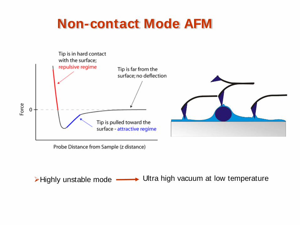
Non-contact Mode AFM
Highly unstable mode Ultra high vacuum at low temperature
Tapping mode AFM
•A cantilever with attached tip is oscillated at its resonant frequency and scanned across the sample surface
•A constant oscillation amplitude (and thus a constant tip-sample interaction) are maintained during scanning. Typical amplitudes are 20-100 nm
•Forces can be 200 pN or less
•The amplitue of the oscillations changes when the tip scans over bumps or depressions on a surface
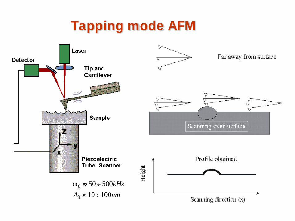
Tapping mode AFM
nmAkHz
1001050050
0
0
÷≈÷≈ω
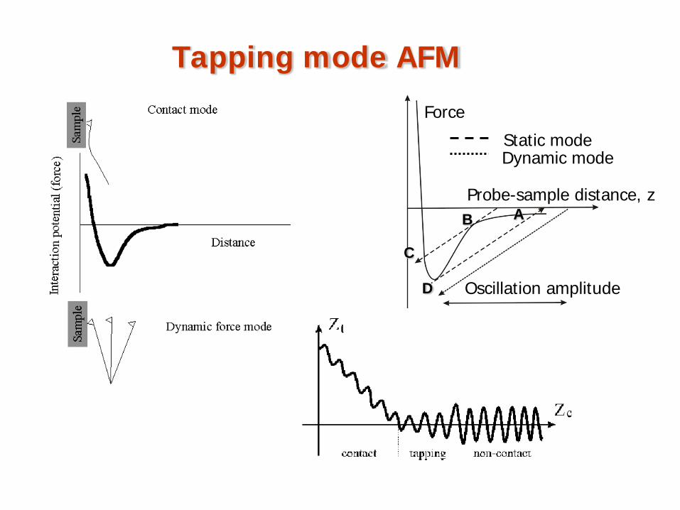
Force
Oscillation amplitude
Probe-sample distance, zAB
C
D
Static modeDynamic mode
Tapping mode AFM
Tapping mode AFM
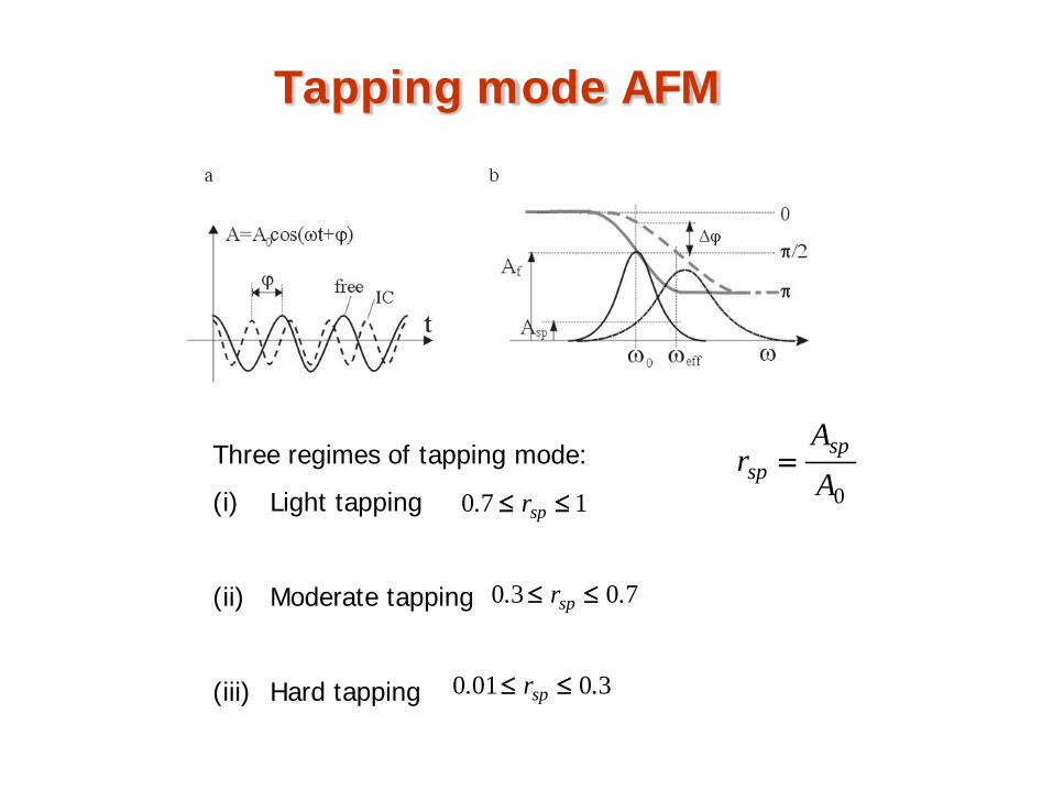
0AA
r spsp =Three regimes of tapping mode:
(i) Light tapping
(ii) Moderate tapping
(iii) Hard tapping
170 ≤≤ spr.
7030 .r. sp ≤≤
30010 .r. sp ≤≤
Tapping mode AFM
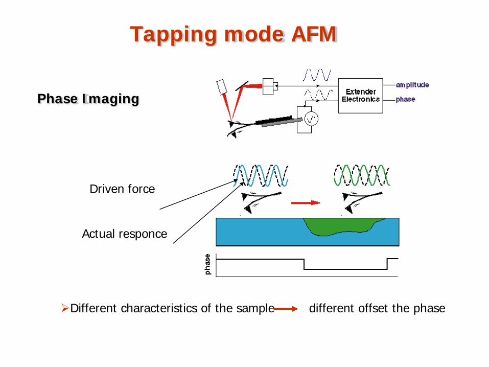
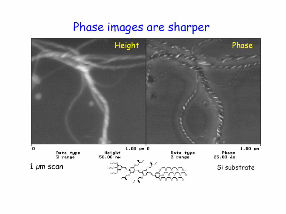
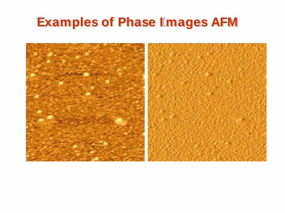
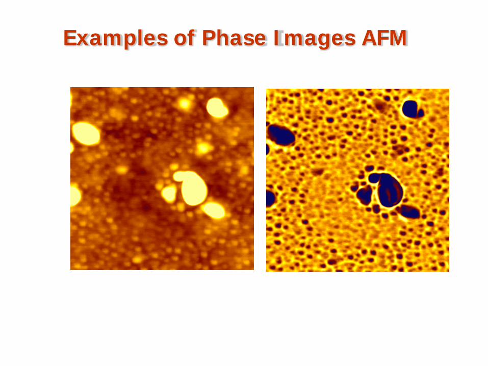
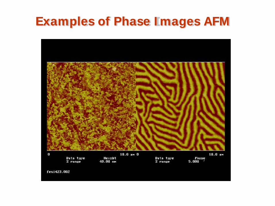
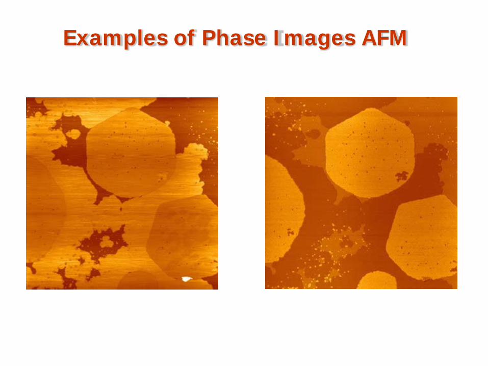
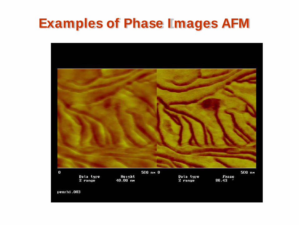
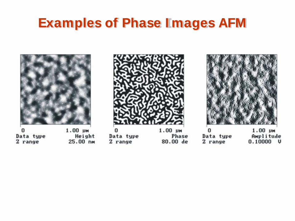
Phase Imaging
Driven force
Actual responce
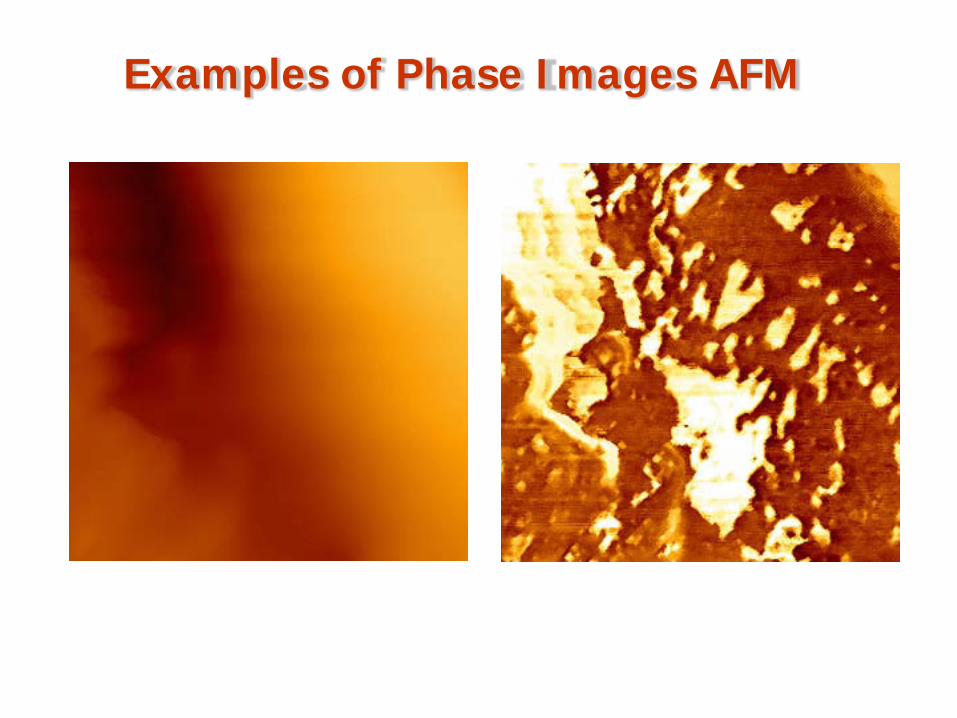
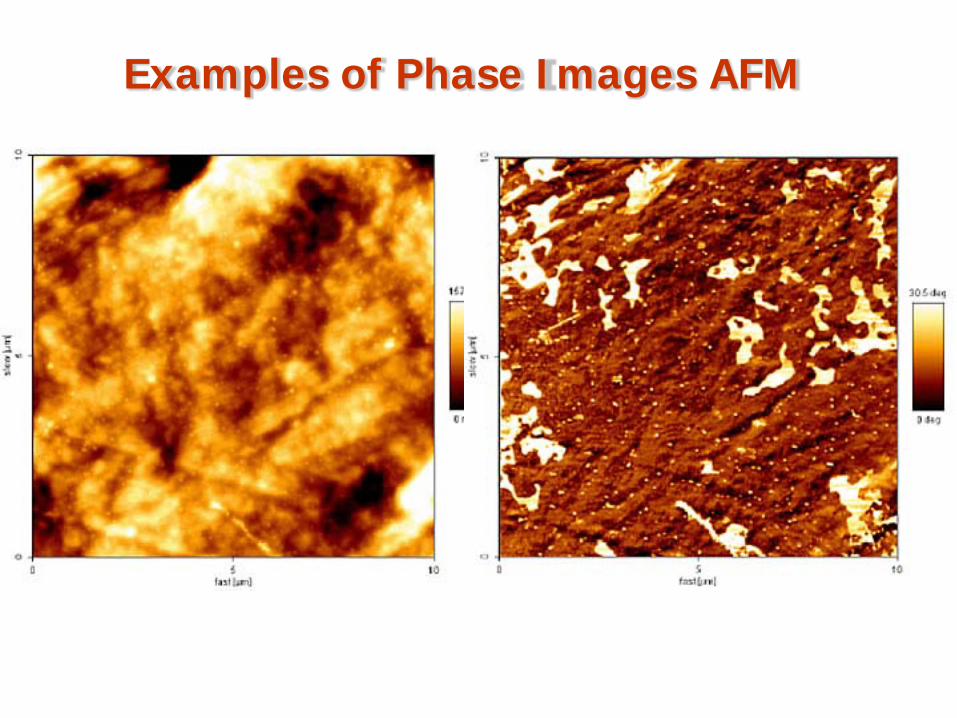
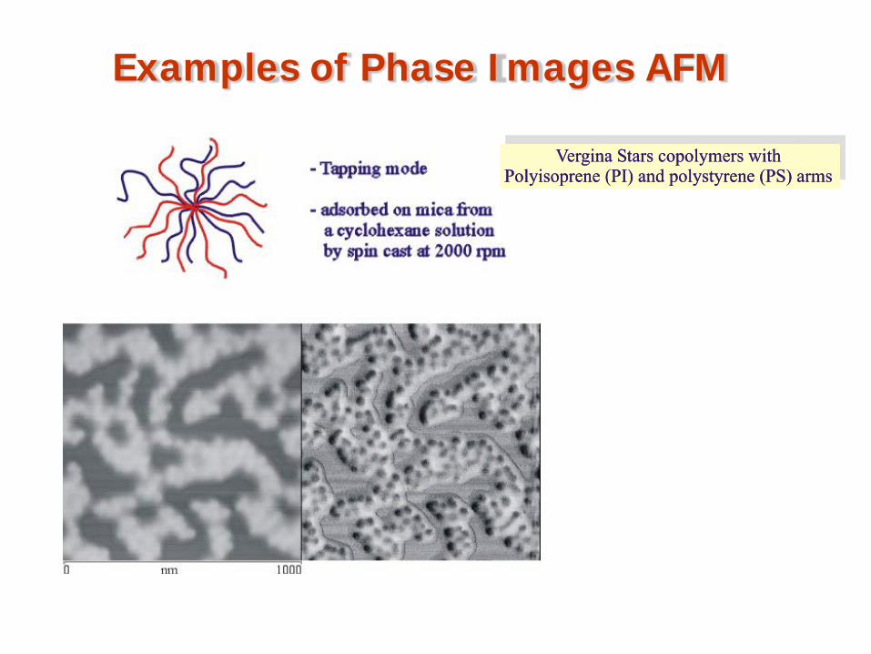
Different characteristics of the sample different offset the phase
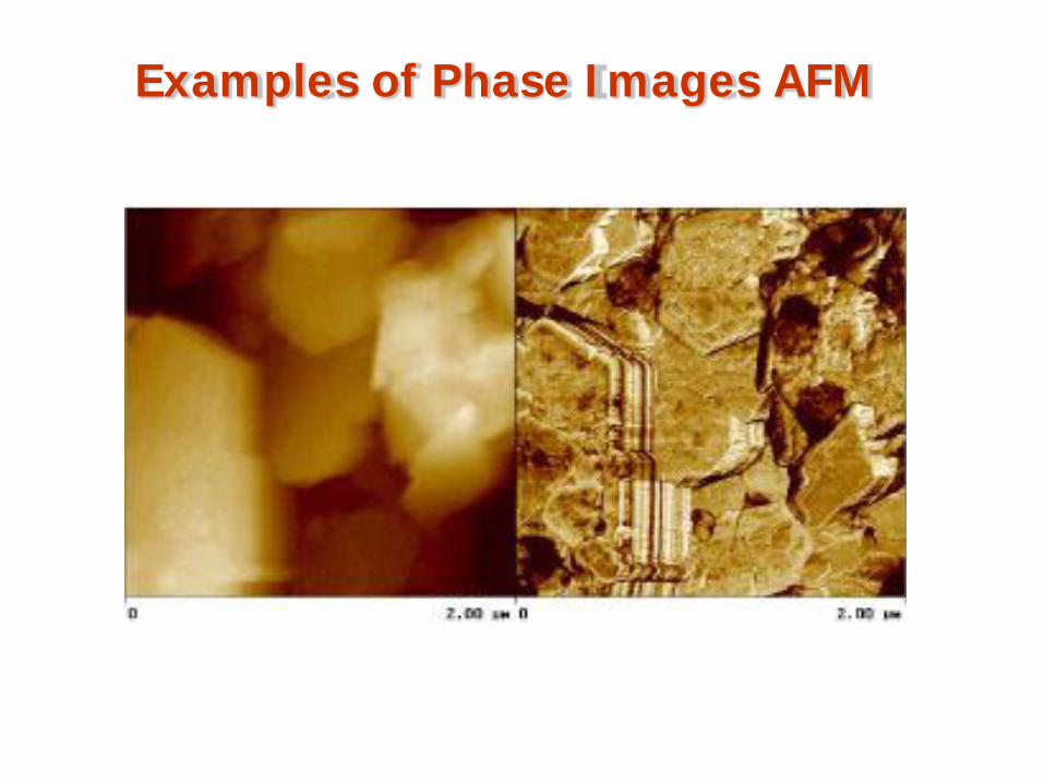
Examples of Phase Images AFM
Examples of Phase Images AFM
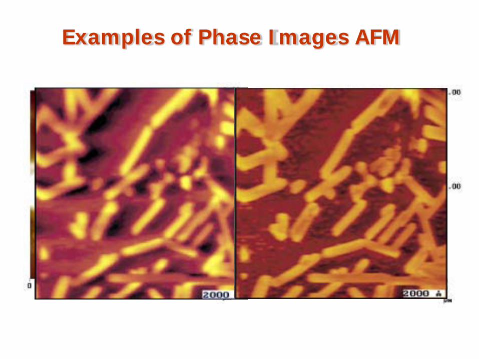
Examples of Phase Images AFM
Examples of Phase Images AFM
Examples of Phase Images AFM
Examples of Phase Images AFM
Examples of Phase Images AFM
Examples of Phase Images AFM
Examples of Phase Images AFM
Examples of Phase Images AFM
Examples of Phase Images AFM
Advantages and DisadvantagesContact Mode
Advantages
high scan speeds
the only mode that can obtain „atomic resolution“ images
rough samples with extreme changes in topography can sometimes be scanned more easily
Disadvantages
lateral (shear) forces can distort features in the images
the forces normal to the tip-sample interction can be high in air due to capillary forces from the adsorbed fluid layer on the sample surface
the combination of lateral forces and high normal forces can result in reduced spatials resolution and may damage soft samples (i.e. biological samples, polymers) due to scraping
Advantages and Disadvantages
Tapping mode
Advantages
higher lateral resolution on most samples (1 to 5 nm)
lower forces and less damage to soft samples imaged in air
lateral forces are virtually eliminated so there is no scraping
Disadvantages
slightly lower scan speed than contact mode AFM
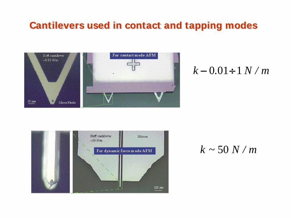
m/N.k 1010 ÷−
m/N~k 50
Cantilevers used in contact and tapping modes
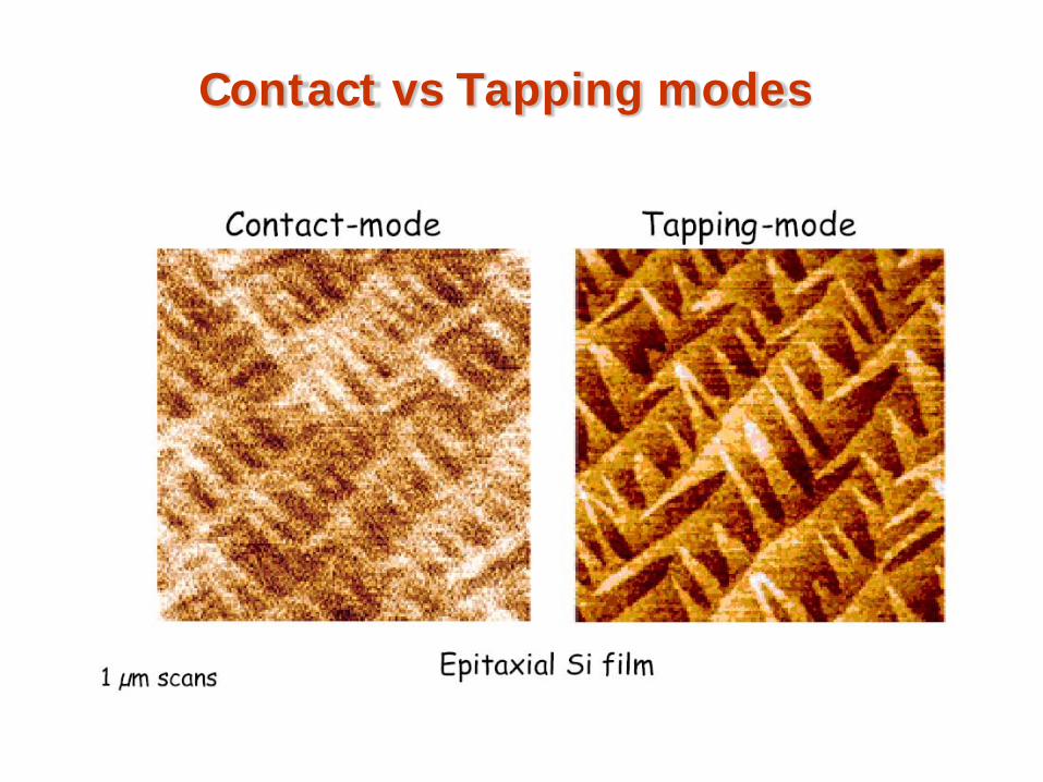
Contact vs Tapping modes
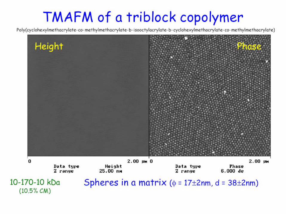
How to interpret height and phase TM-AFM images of a sample in
terms of its physical and morphological properties?