Spin-orbit coupling in Wien2k

Robert Laskowskirolask@ihpc.a-star.edu.sg

Institute of High Performance Computing

Singapore

2

Dirac Hamiltonian

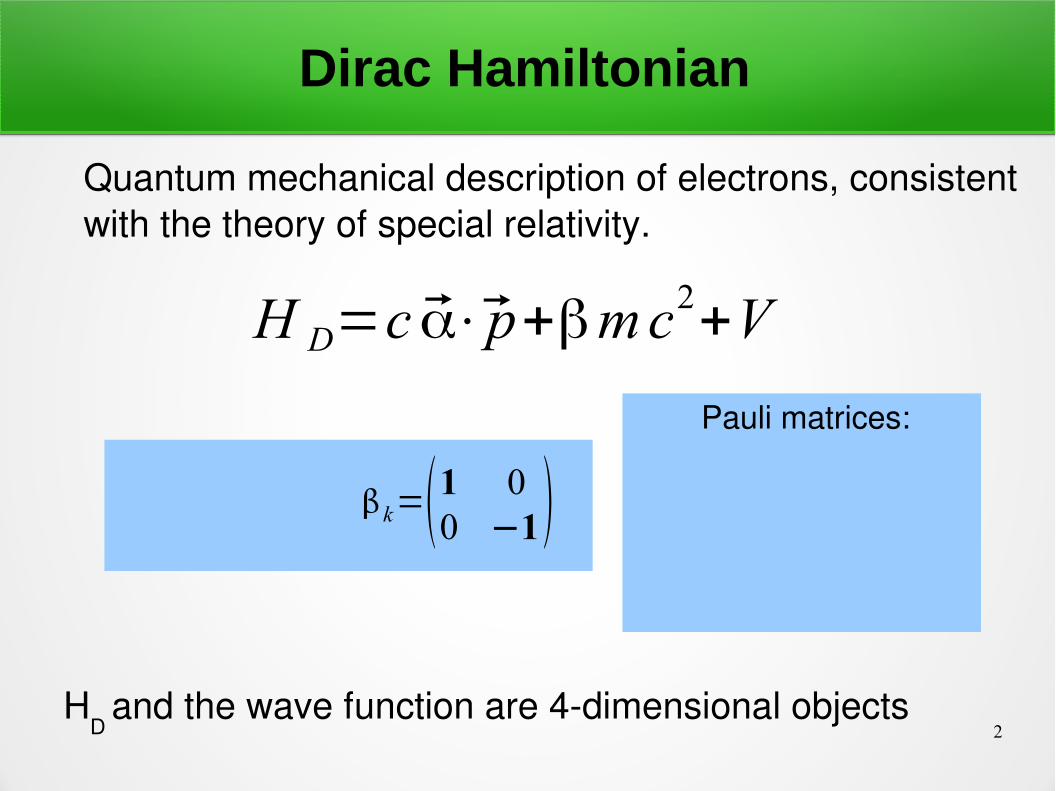
H D=c α⃗⋅p⃗+βmc2+V

Quantum mechanical description of electrons, consistent with the theory of special relativity.

k= 0 k

k 0 1=0 11 0 , 2=0 −i

i 0 , 3=1 0

0 −1k=1 0

0 −1Pauli matrices:

HD 

and the wave function are 4­dimensional objects

3

Dirac Hamiltonian

H D 1234=

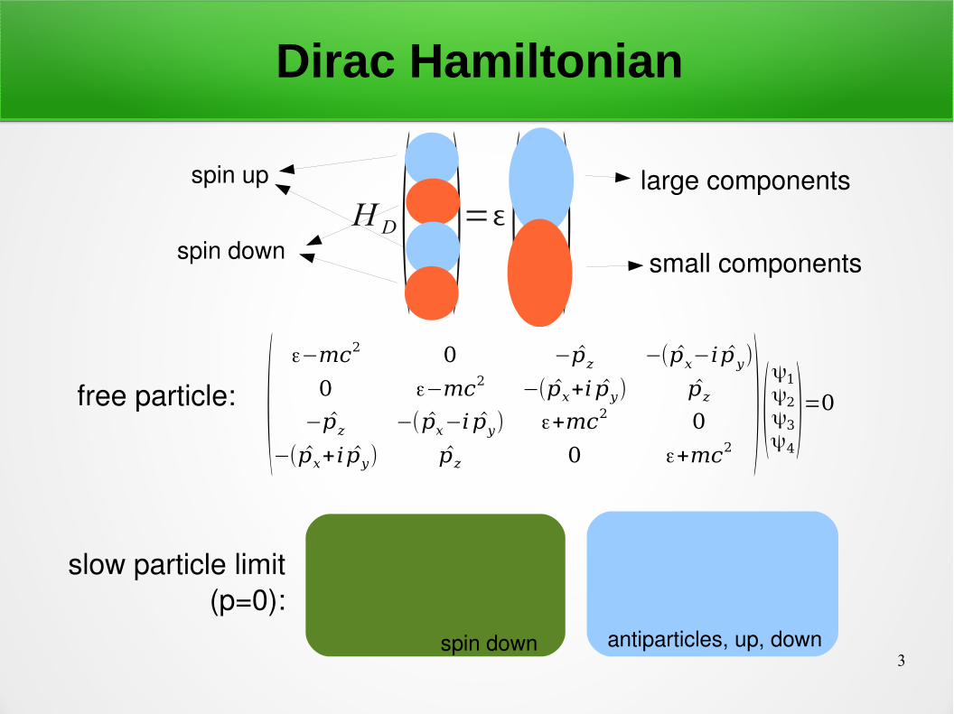
123 4 large components

small components

spin up

spin down

(ε−mc2 0 −p̂z −(p̂x−i p̂ y)

0 ε−mc2 −(p̂x+i p̂y) p̂z

−p̂z −(p̂x−i p̂y) ε+mc2 0

−(p̂x+i p̂y) p̂z 0 ε+mc2)(ψ1ψ2ψ3ψ4)=0

slow particle limit (p=0):

free particle:

mc2 , 000 mc2 ,

000 −mc2 ,

000 −mc2 ,

000

spin up spin down antiparticles, up, down

4

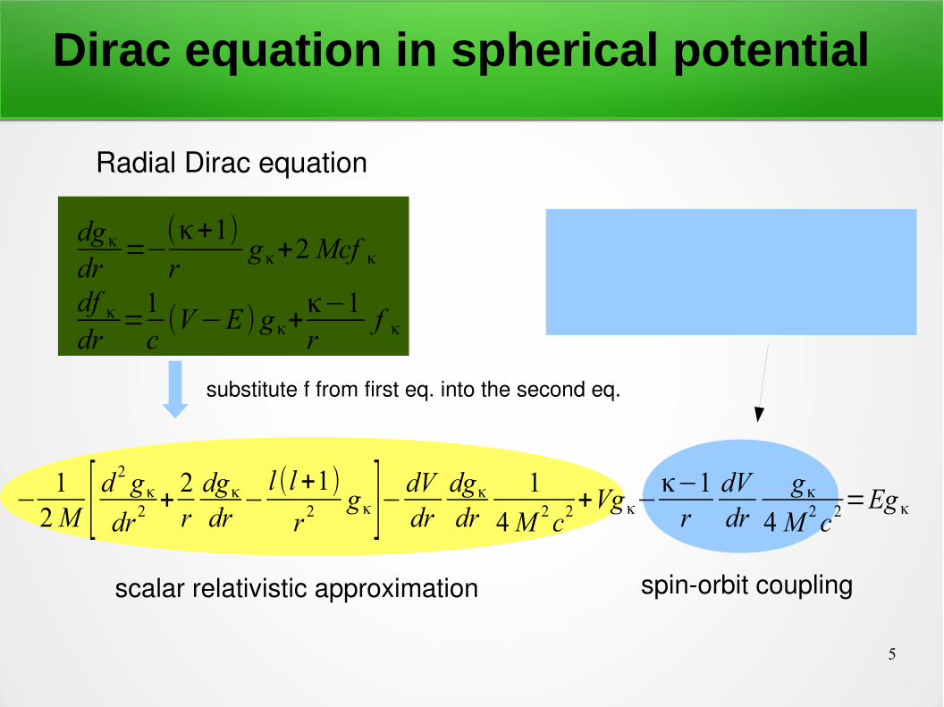
Dirac equation in spherical potential

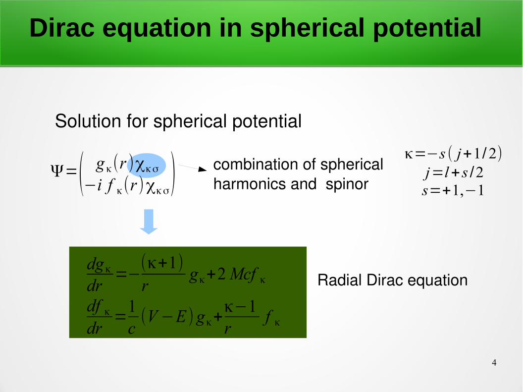
Ψ=( g κ(r )χκσ−i f κ(r )χκσ)

κ=−s ( j+1/2)j=l+s /2s=+1,−1

dgκdr

=−(κ+1)r

gκ+2Mcf κ

df κdr=1c(V−E ) gκ+

κ−1r

f κ

Solution for spherical potential

combination of spherical harmonics and  spinor 

Radial Dirac equation

5

Dirac equation in spherical potential

dgκdr

=−(κ+1)r

gκ+2Mcf κ

df κdr=1c(V−E ) gκ+

κ−1r

f κ

−12M [ d

2 gκdr 2

+2rdgκdr−l (l+1)

r 2gκ]− dV

drdgκdr

1

4M 2c2+Vgκ−

κ−1r

dVdr

gκ4M 2c2

=Eg κ

substitute f from first eq. into the second eq.

Radial Dirac equation

scalar relativistic approximation spin­orbit coupling

κ dependent term, for a constant l, κ depends on the sign of s

6

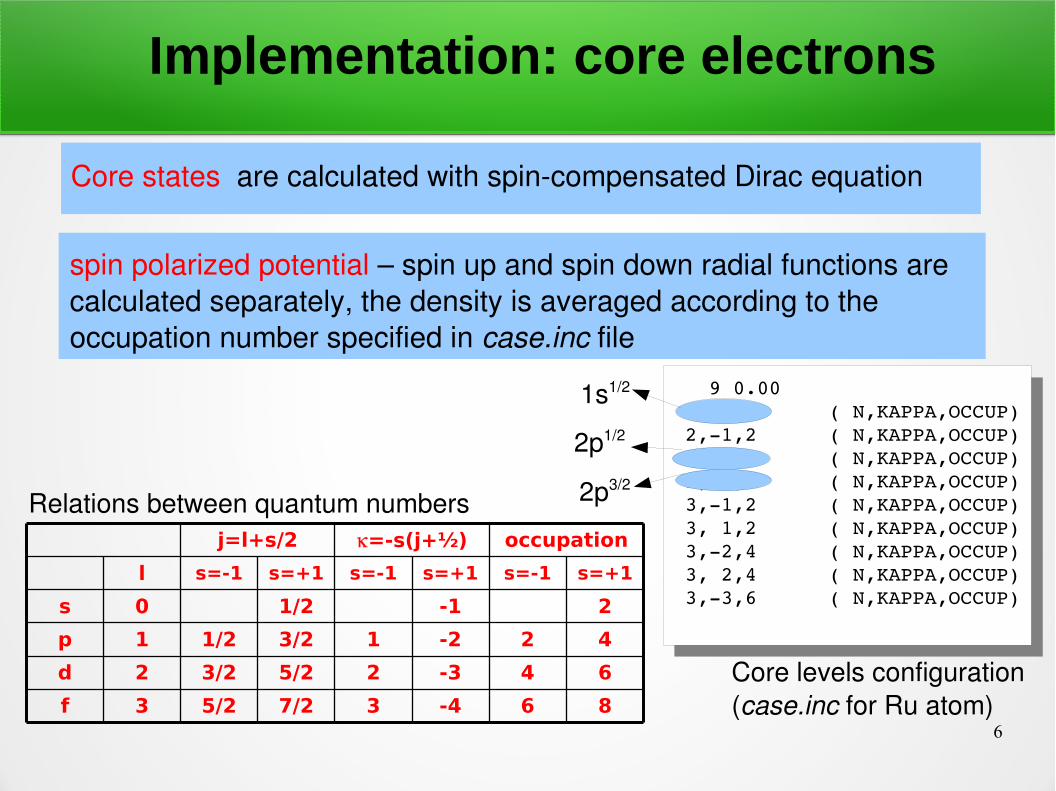
Implementation: core electrons

Core states  are calculated with spin­compensated Dirac equation

spin polarized potential – spin up and spin down radial functions are calculated separately, the density is averaged according to the occupation number specified in case.inc file 

  9 0.00     1,­1,2      ( N,KAPPA,OCCUP)2,­1,2      ( N,KAPPA,OCCUP)2, 1,2      ( N,KAPPA,OCCUP)2,­2,4      ( N,KAPPA,OCCUP)3,­1,2      ( N,KAPPA,OCCUP)3, 1,2      ( N,KAPPA,OCCUP)3,­2,4      ( N,KAPPA,OCCUP)3, 2,4      ( N,KAPPA,OCCUP)3,­3,6      ( N,KAPPA,OCCUP)

Core levels configuration (case.inc for Ru atom)86-437/25/23f

64-325/23/22d

42-213/21/21p

2-11/20s

s=+1s=-1s=+1s=-1s=+1s=-1l

occupation=-s(j+½)j=l+s/2

1s1/2

2p1/2

2p3/2Relations between quantum numbers

7

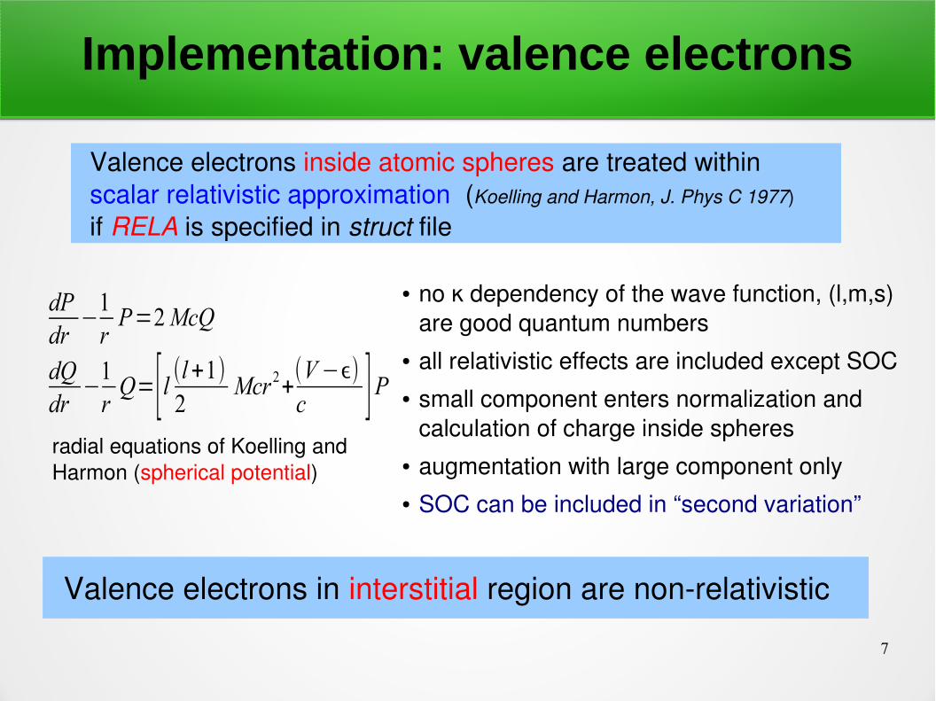
Implementation: valence electrons

Valence electrons inside atomic spheres are treated within scalar relativistic approximation  (Koelling and Harmon, J. Phys C 1977) 

if RELA is specified in struct file

radial equations of Koelling and Harmon (spherical potential)

dPdr−1rP=2McQ

dQdr−1rQ=[l (l+1)2

Mcr2+(V−ϵ)c ]P

● no   dependency of the wave function, (l,m,s) κare good quantum numbers  

● all relativistic effects are included except SOC ● small component enters normalization and 

calculation of charge inside spheres● augmentation with large component only● SOC can be included in “second variation”

Valence electrons in interstitial region are non­relativistic

8

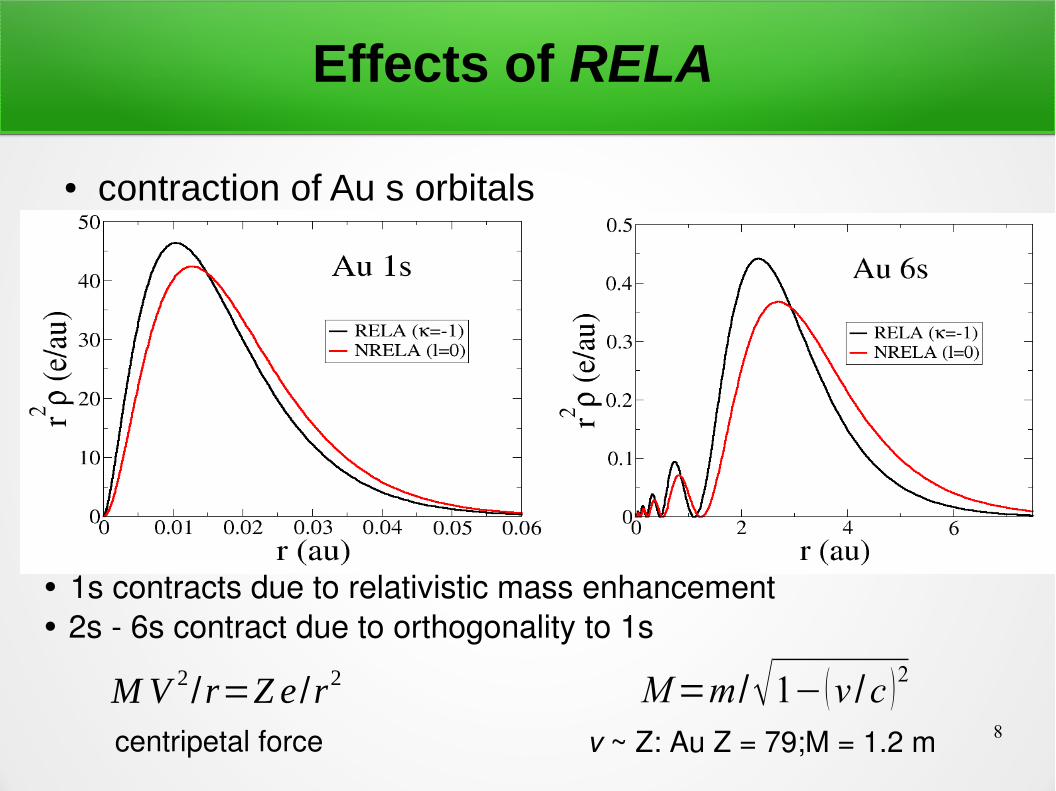
Effects of RELA

● contraction of Au s orbitals

• 1s contracts due to relativistic mass enhancement• 2s ­ 6s contract due to orthogonality to 1s

v ~ Z: Au Z = 79;M = 1.2 m

M=m /√1−(v /c )2M V 2/r=Z e /r2

centripetal force

9

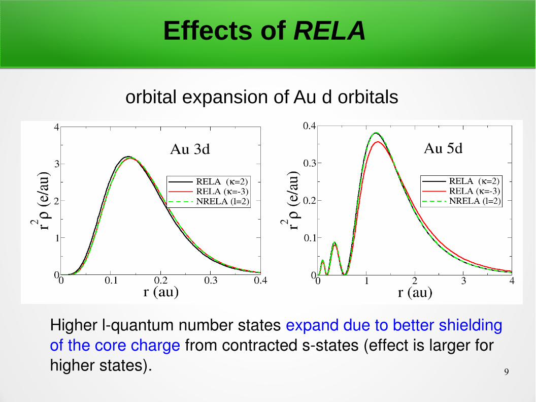
Effects of RELA

orbital expansion of Au d orbitals

Higher l­quantum number states expand due to better shielding of the core charge from contracted s­states (effect is larger for higher states).

10

Spin orbit-coupling

=1

2Mc21

r2dV MT r

drH P=−ℏ

2m∇2V ef ⋅l

x=0 11 0

Pauli matrices:

y=0 −ii 0

z=1 00 −1

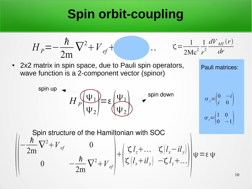
● 2x2 matrix in spin space, due to Pauli spin operators, wave function is a 2-component vector (spinor)

H P 12= 12

spin up spin down 

−ℏ

2m∇2V ef 0

0 −ℏ

2m∇2V ef lz lx−il y

lxil y − lz=Spin structure of the Hamiltonian with SOC

11

Spin-orbit coupling

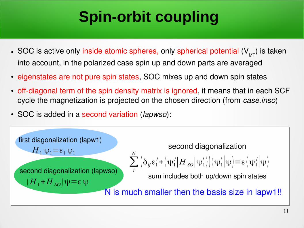
● SOC is active only inside atomic spheres, only spherical potential (VMT

) is taken into account, in the polarized case spin up and down parts are averaged  

● eigenstates are not pure spin states, SOC mixes up and down spin states

● off­diagonal term of the spin density matrix is ignored, it means that in each SCF cycle the magnetization is projected on the chosen direction (from case.inso)

● SOC is added in a second variation (lapwso):

H 1ψ1=ε1ψ1

∑i

N

(δ ijε1j+ ⟨ψ1j|H SO|ψ1i ⟩ ) ⟨ψ1i|ψ ⟩=ε ⟨ψ1j|ψ ⟩

first diagonalization (lapw1)

(H 1+H SO )ψ=εψsecond diagonalization (lapwso)

second diagonalization

sum includes both up/down spin states 

N is much smaller then the basis size in lapw1!!

12

SOC splitting of p states

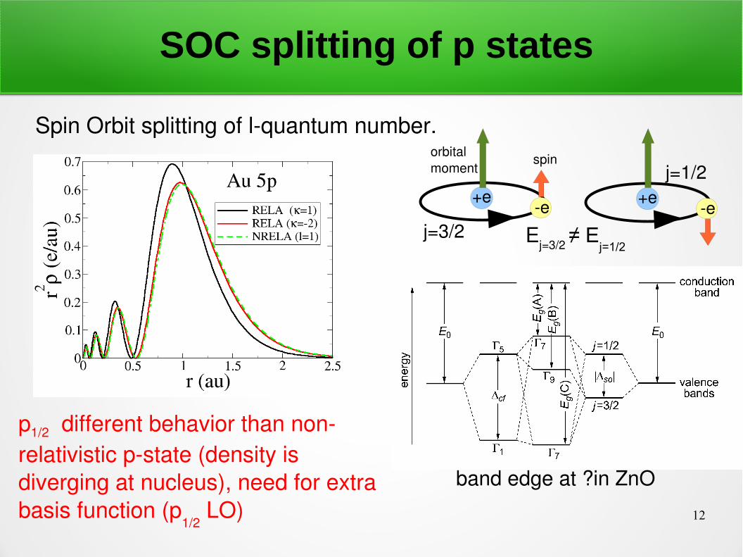
p1/2  different behavior than non­relativistic p­state (density is diverging at nucleus), need for extra basis function (p

1/2 LO)

Spin Orbit splitting of l­quantum number.

+e­e

orbital moment

spin

Ej=3/2 ≠ Ej=1/2

+e­e

band edge at ? in ZnO

j=3/2

j=1/2

13

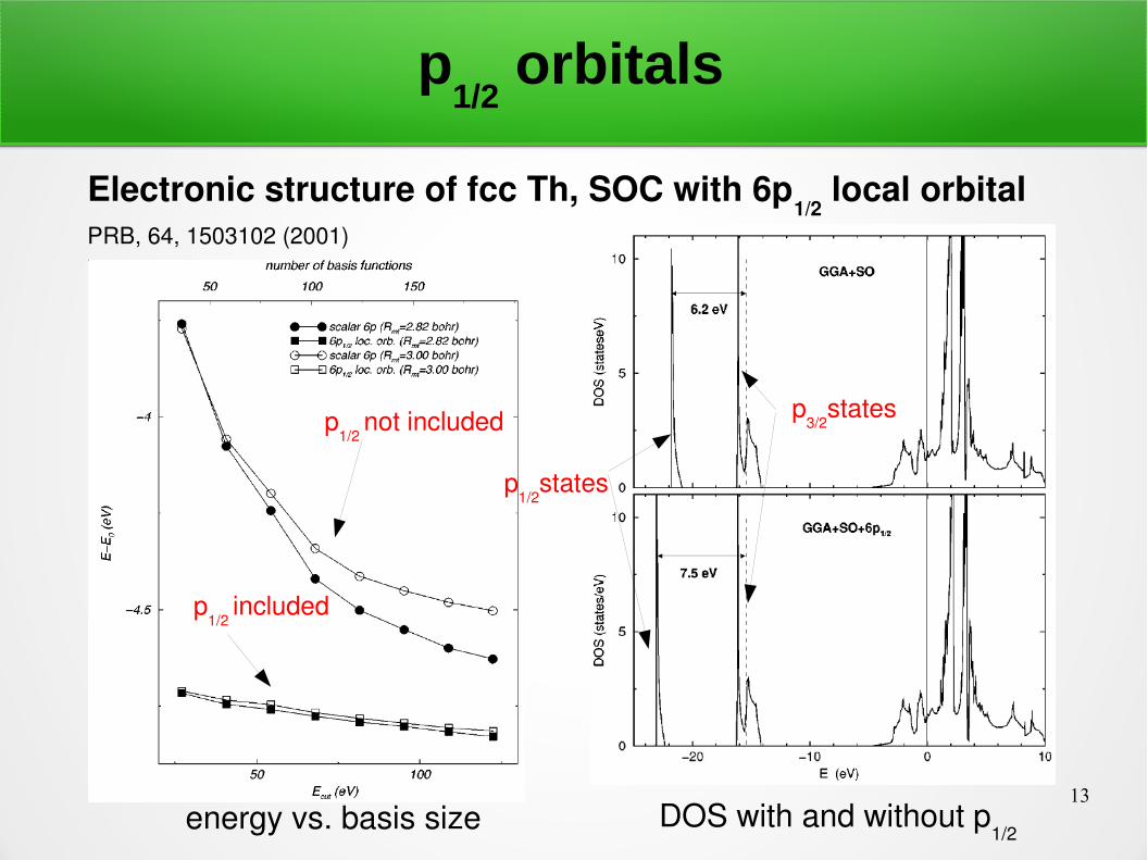
p1/2

orbitals

Electronic structure of fcc Th, SOC with 6p1/2

 local orbitalPRB, 64, 1503102 (2001)

energy vs. basis size DOS with and without p1/2

p1/2 

included

p1/2 

not included  p3/2

states

p1/2

states

14

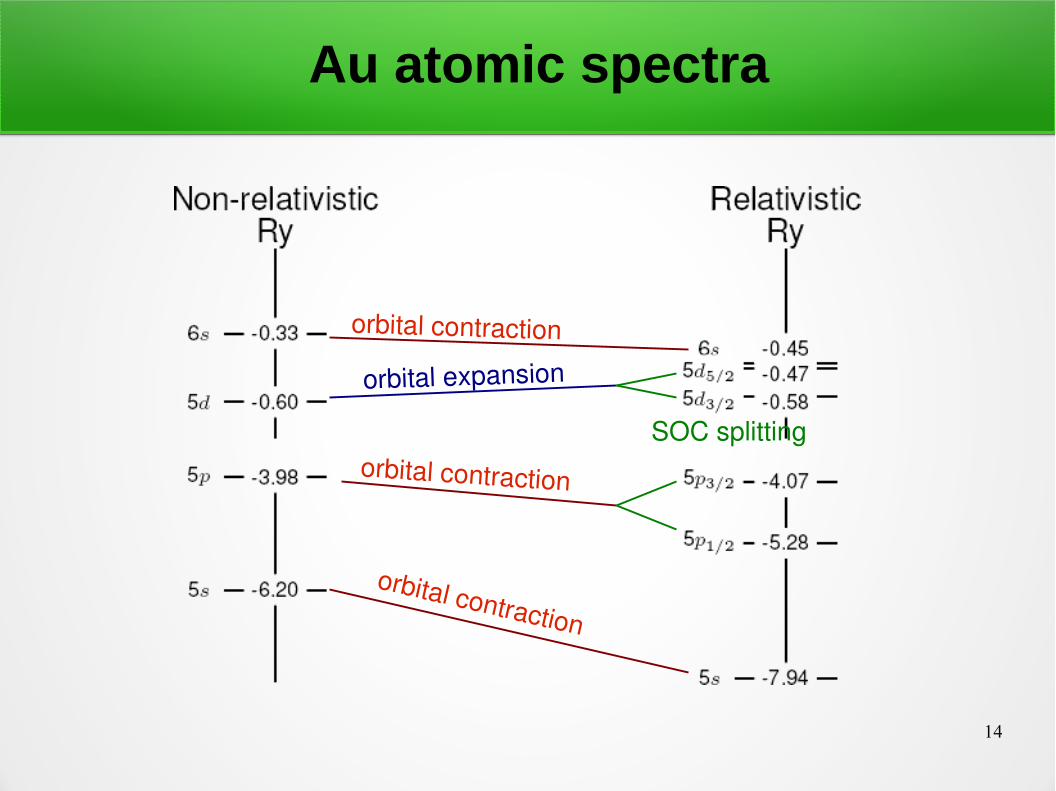
Au atomic spectra

orbital contraction

orbital contraction

orbital contraction

orbital expansion

SOC splitting

15

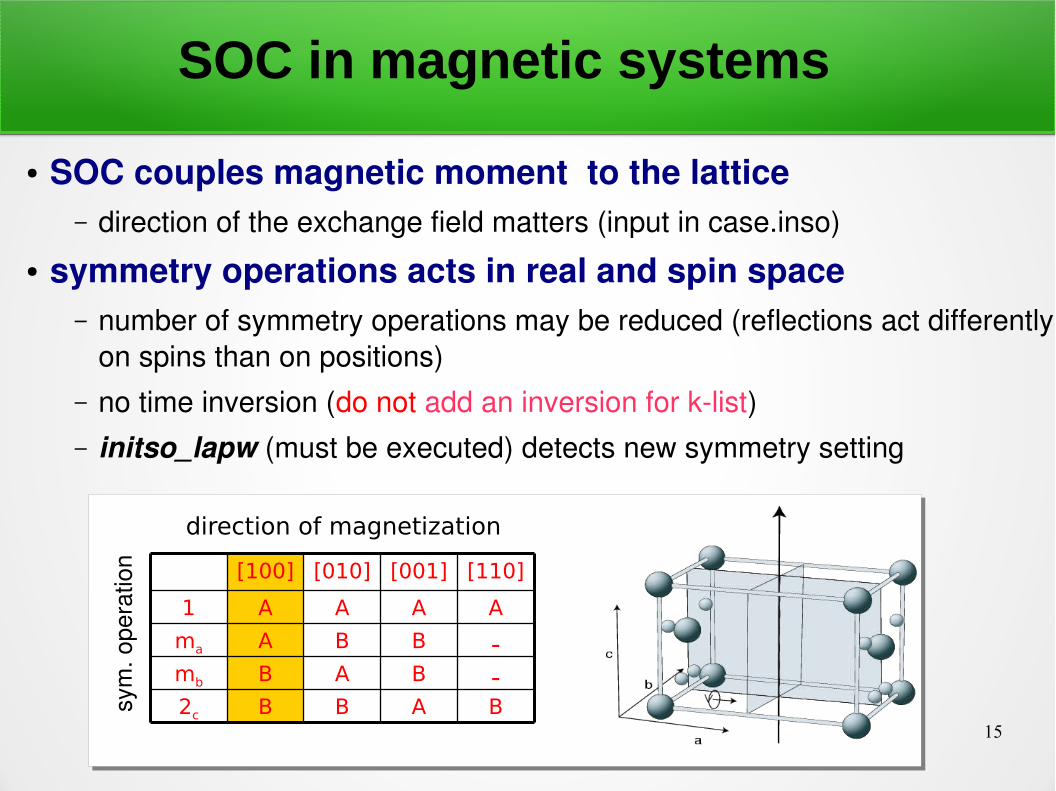
SOC in magnetic systems

● SOC couples magnetic moment  to the lattice– direction of the exchange field matters (input in case.inso)

● symmetry operations acts in real and spin space – number of symmetry operations may be reduced (reflections act differently 

on spins than on positions)– no time inversion (do not add an inversion for k­list)– initso_lapw (must be executed) detects new symmetry setting

BABB2c

-BABmb

-BBAma

AAAA1

[110][001][010][100]

direction of magnetization

sym

. ope

ratio

n

16

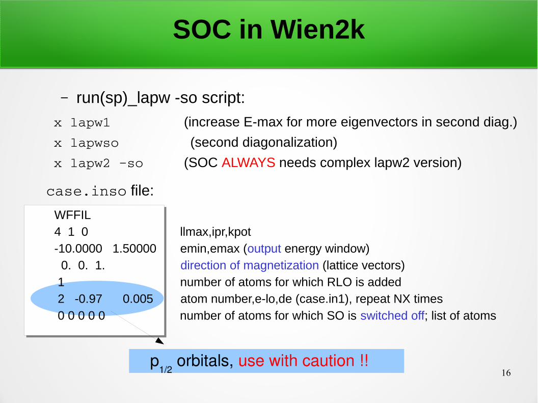
SOC in Wien2k

x lapw1         (increase E-max for more eigenvectors in second diag.)

x lapwso (second diagonalization)

x lapw2 –so     (SOC ALWAYS needs complex lapw2 version)

– run(sp)_lapw -so script:

case.inso file:

WFFIL4 1 0 llmax,ipr,kpot -10.0000 1.50000 emin,emax (output energy window) 0. 0. 1. direction of magnetization (lattice vectors) 1 number of atoms for which RLO is added 2 -0.97 0.005 atom number,e-lo,de (case.in1), repeat NX times 0 0 0 0 0 number of atoms for which SO is switched off; list of atoms

p1/2

 orbitals, use with caution !! 

17

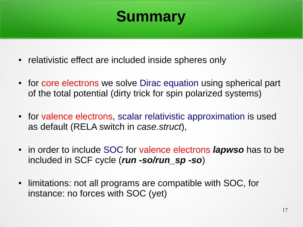
Summary

● relativistic effect are included inside spheres only

● for core electrons we solve Dirac equation using spherical part of the total potential (dirty trick for spin polarized systems)

● for valence electrons, scalar relativistic approximation is used as default (RELA switch in case.struct),

● in order to include SOC for valence electrons lapwso has to be included in SCF cycle (run -so/run_sp -so)

● limitations: not all programs are compatible with SOC, for instance: no forces with SOC (yet)

18

NCM

19

Pauli Hamiltonian

H P=−ℏ2m∇2V efB ⋅ Bef⋅l

2x2 matrix in spin space, due to Pauli spin operators wave function is a 2­component vector (spinor)

H P 12= 12

spin up component

spin down component

1=0 11 0

Pauli matrices:

2=0 −ii 0

3=1 00 −1

V ef=V extV HV xc Bef=BextBxc

Hartee term exchange­correlation potential

exchange­correlation field

20

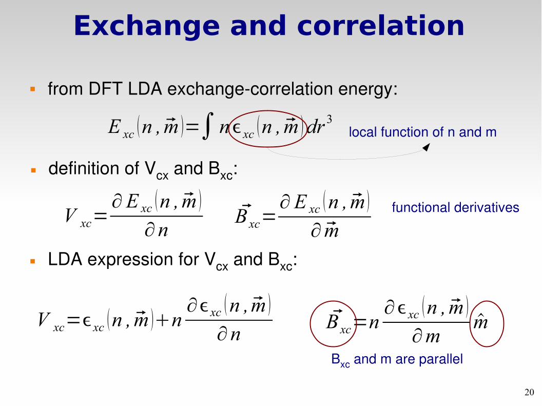
Exchange and correlation

from DFT LDA exchange­correlation energy:

E xc n , m =∫nxc n , m dr 3

definition of Vcx and Bxc:

V xc=∂E xc n , m

∂nBxc=

∂E xc n , m

∂ m LDA expression for Vcx and Bxc:

V xc=xc n , m n∂xc n , m

∂nBxc=n

∂xc n , m

∂mm

local function of n and m

functional derivatives

Bxc and m are parallel

21

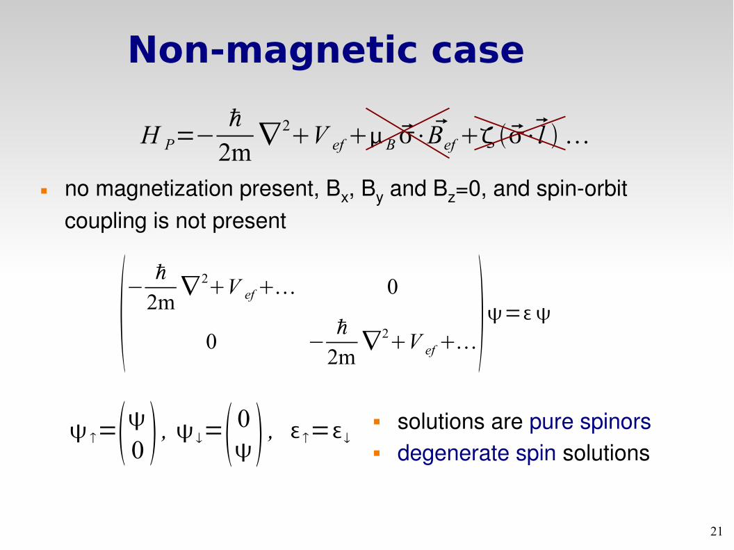
Non-magnetic case

no magnetization present, Bx, By and Bz=0, and spin­orbit coupling is not present  

H P=−ℏ

2m∇2V efB ⋅ Bef⋅l

−ℏ

2m∇2V ef 0

0 −ℏ

2m∇2V ef=

=0 , = 0 , = solutions are pure spinors degenerate spin solutions  

22

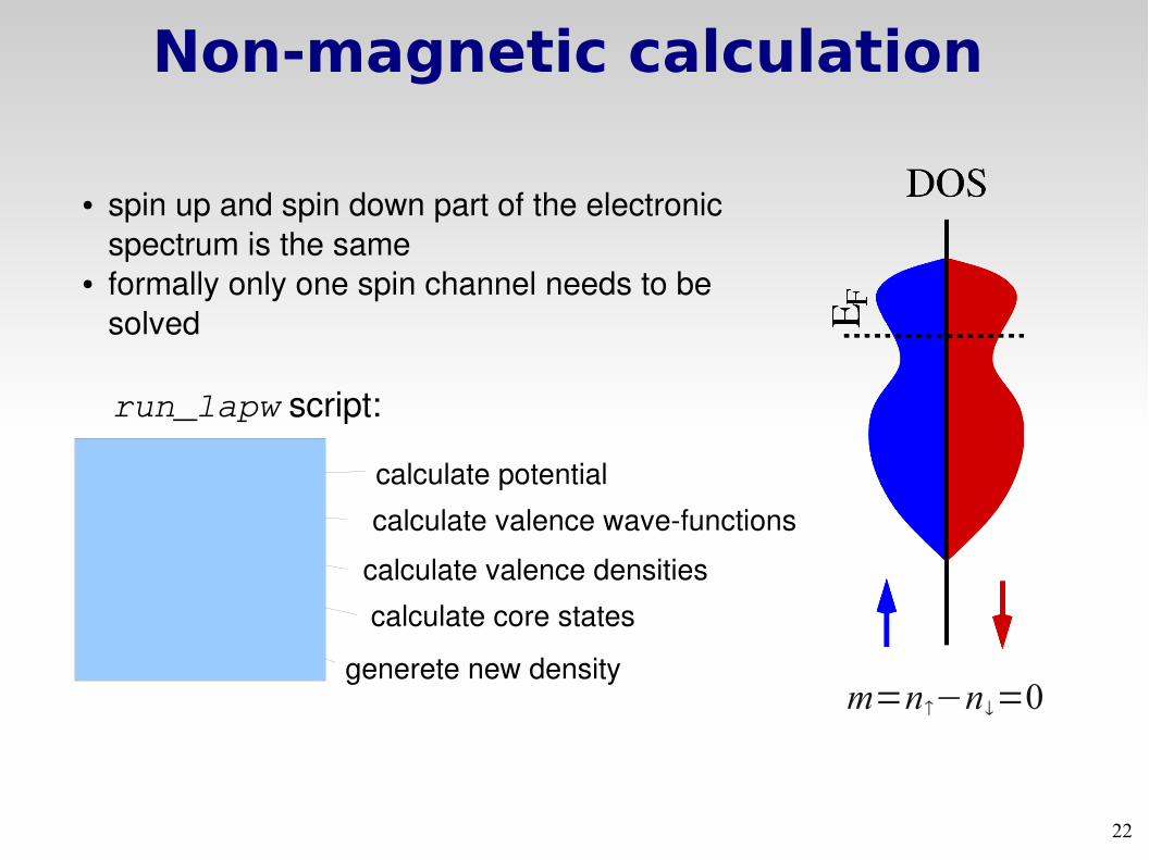
Non-magnetic calculation

run_lapw script:

x lapw0x lapw1x lapw2x lcorex mixer

m=n−n=0generete new density

calculate core states

calculate valence densities

calculate valence wave­functions

calculate potential

● spin up and spin down part of the electronic spectrum is the same

● formally only one spin channel needs to be solved

23

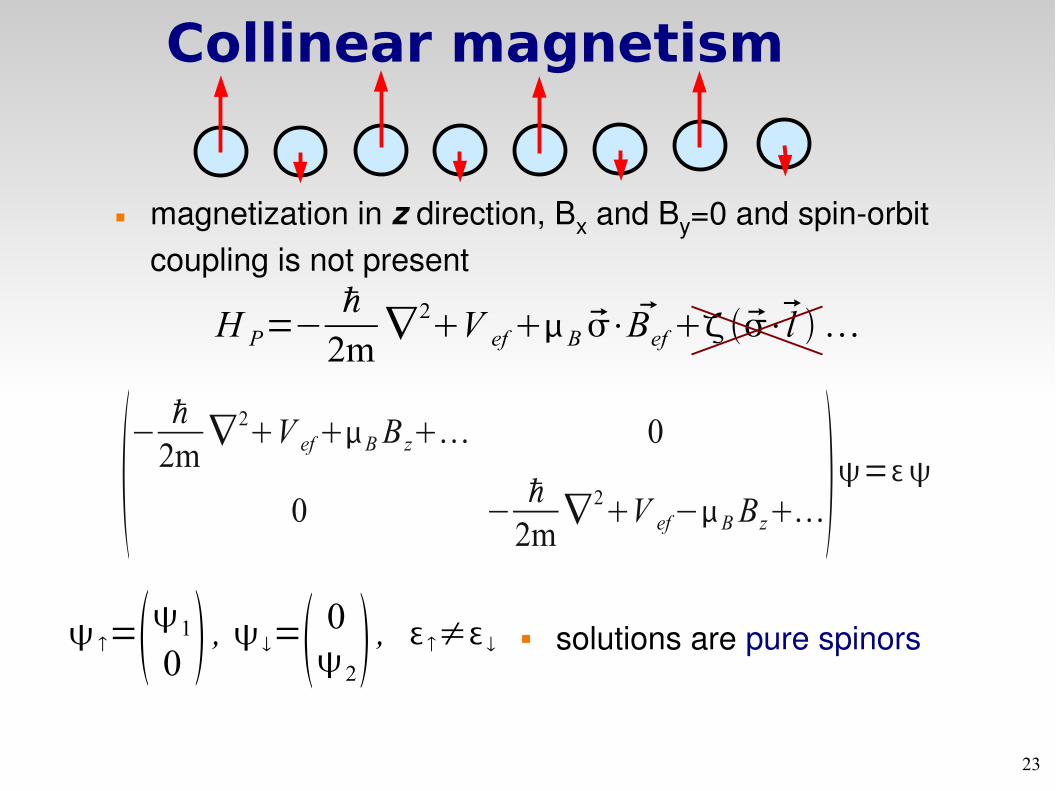
Collinear magnetism

magnetization in z direction, Bx and By=0 and spin­orbit coupling is not present  

H P=−ℏ

2m∇2V efB ⋅ Bef⋅l

−ℏ

2m∇2V efBB z 0

0 −ℏ

2m∇2V ef−BBz=

=10 , = 02 , ≠ solutions are pure spinors  

24

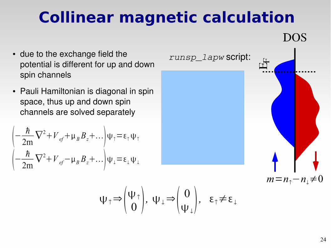
Collinear magnetic calculation

runsp_lapw script:

x lapw0x lapw1 ­upx lapw1 ­dnx lapw2 ­upx lapw2 ­dnx lcore ­upx lcore ­dnx mixer

m=n−n≠0

● due to the exchange field the potential is different for up and down spin channels

● Pauli Hamiltonian is diagonal in spin space, thus up and down spin channels are solved separately 

− ℏ2m∇2V efBBz =

− ℏ

2m∇2V ef−B Bz =

⇒ 0 , ⇒ 0 , ≠

25

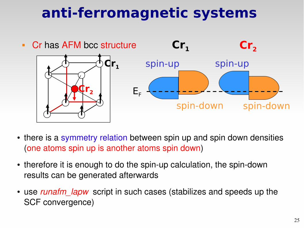
anti-ferromagnetic systems

Cr has AFM bcc structure 

Cr1

Cr2

Cr1 Cr2

spin-up spin-up

spin-down spin-down

EF

● there is a symmetry relation between spin up and spin down densities (one atoms spin up is another atoms spin down)

● therefore it is enough to do the spin­up calculation, the spin­down results can be generated afterwards

● use runafm_lapw  script in such cases (stabilizes and speeds up the SCF convergence)

26

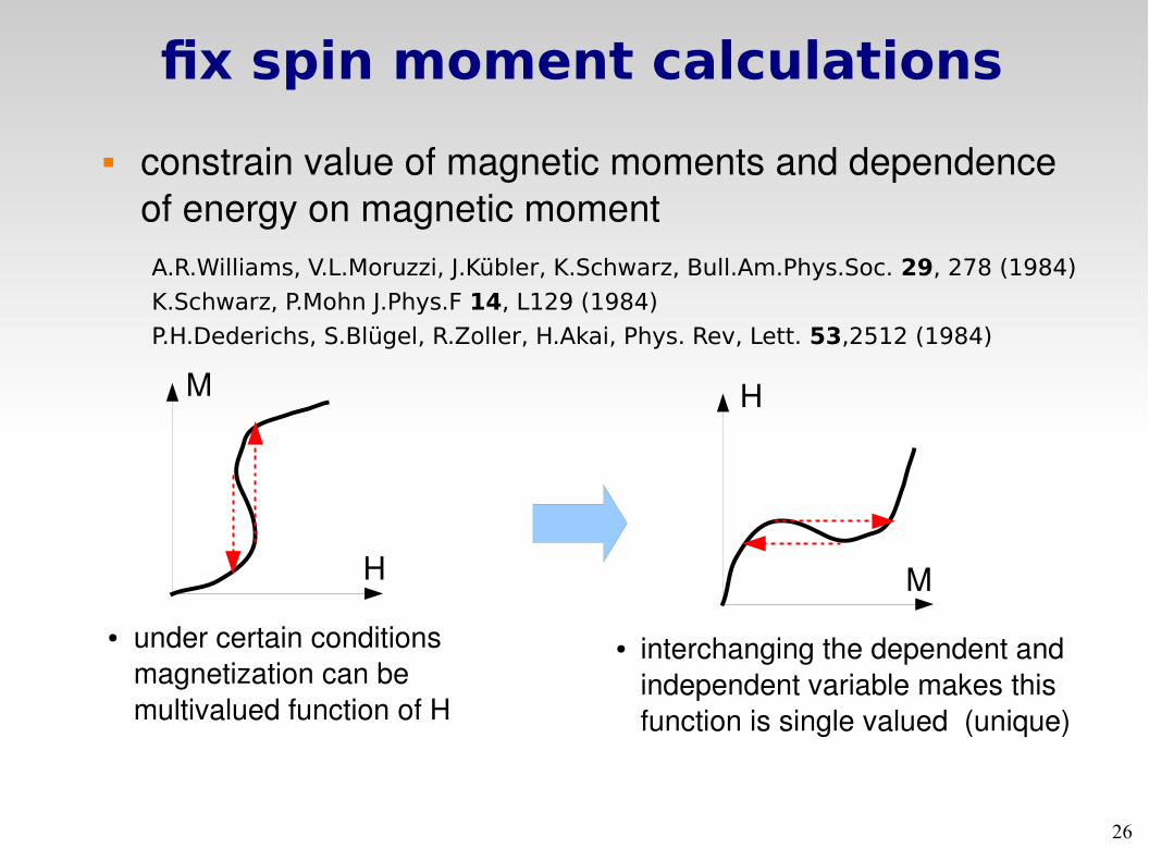
fix spin moment calculations

constrain value of magnetic moments and dependence of energy on magnetic moment  A.R.Williams, V.L.Moruzzi, J.Kübler, K.Schwarz, Bull.Am.Phys.Soc. 29, 278 (1984)

K.Schwarz, P.Mohn J.Phys.F 14, L129 (1984)

P.H.Dederichs, S.Blügel, R.Zoller, H.Akai, Phys. Rev, Lett. 53,2512 (1984)

H

M

● under certain conditions magnetization can be multivalued function of H

H

M

● interchanging the dependent and independent variable makes this function is single valued  (unique)

27

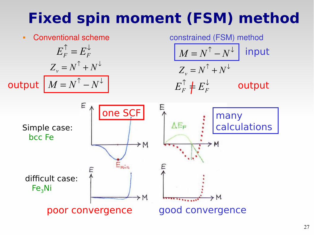
Fixed spin moment (FSM) method Conventional scheme  constrained (FSM) method

FF EE NNZv

NNMoutput FF EE

NNZv

NNM input

output

poor convergence good convergence

Simple case:bcc Fe

difficult case:Fe3Ni

one SCF many calculations

28

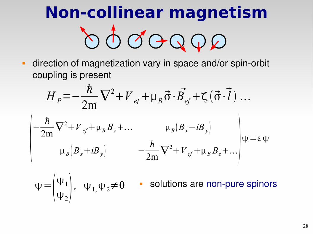
Non-collinear magnetism

direction of magnetization vary in space and/or spin­orbit coupling is present  

−ℏ

2m∇ 2V efB B z B B x−iB y

B B xiB y −ℏ

2m∇2V ef B Bz=

=12 , 1,2≠0 solutions are non­pure spinors  

H P=−ℏ2m∇2V efB ⋅ Bef⋅l

29

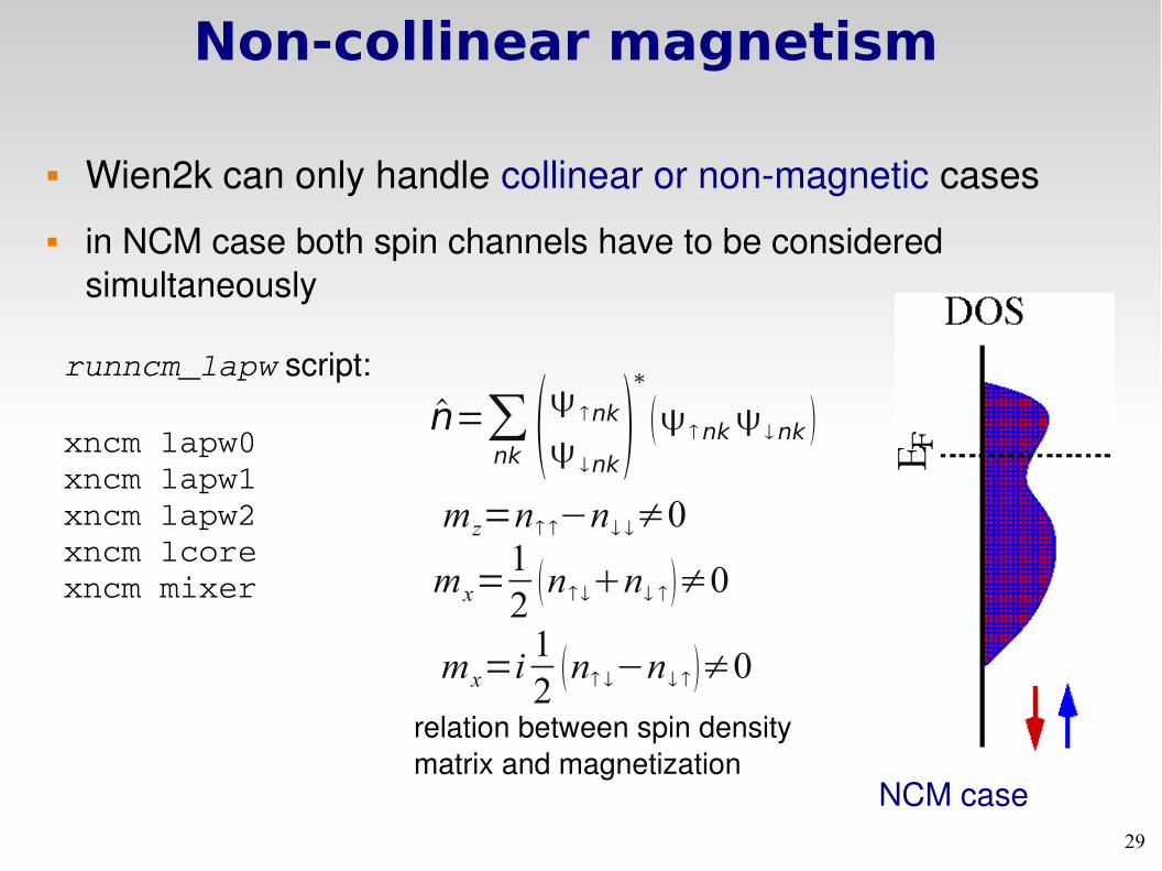
Non-collinear magnetism

Wien2k can only handle collinear or non­magnetic cases in NCM case both spin channels have to be considered 

simultaneously

runncm_lapw script:

xncm lapw0xncm lapw1xncm lapw2xncm lcorexncm mixer

NCM case

mz=n −n ≠0

mx=12 n n ≠0

mx=i12 n −n ≠0

n=∑nk nk nk

∗

nk nk

relation between spin density matrix and magnetization

30

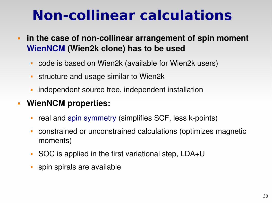
Non-collinear calculations in the case of non­collinear arrangement of spin moment 

WienNCM (Wien2k clone) has to be used

code is based on Wien2k (available for Wien2k users)

structure and usage similar to Wien2k

independent source tree, independent installation

WienNCM properties:

real and spin symmetry (simplifies SCF, less k­points)

constrained or unconstrained calculations (optimizes magnetic moments)

SOC is applied in the first variational step, LDA+U

spin spirals are available

31

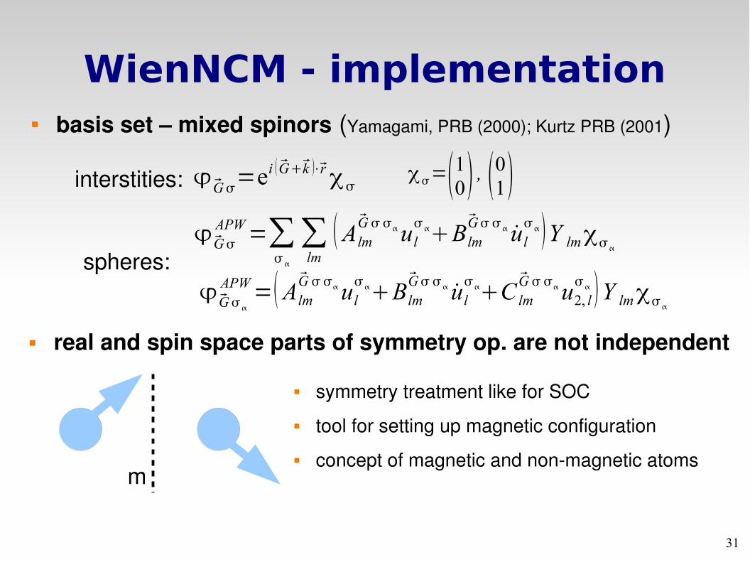
WienNCM - implementation basis set – mixed spinors (Yamagami, PRB (2000); Kurtz PRB (2001)

G=ei

Gk ⋅rinterstities:

spheres: G

APW=∑

∑lmAlm

GulBlm

G u̇lY lm

G

APW=Alm

GulBlm

G u̇lC lm

Gu2, l Y lm

=10 , 01

real and spin space parts of symmetry op. are not independent 

m

symmetry treatment like for SOC

tool for setting up magnetic configuration

concept of magnetic and non­magnetic atoms 

32

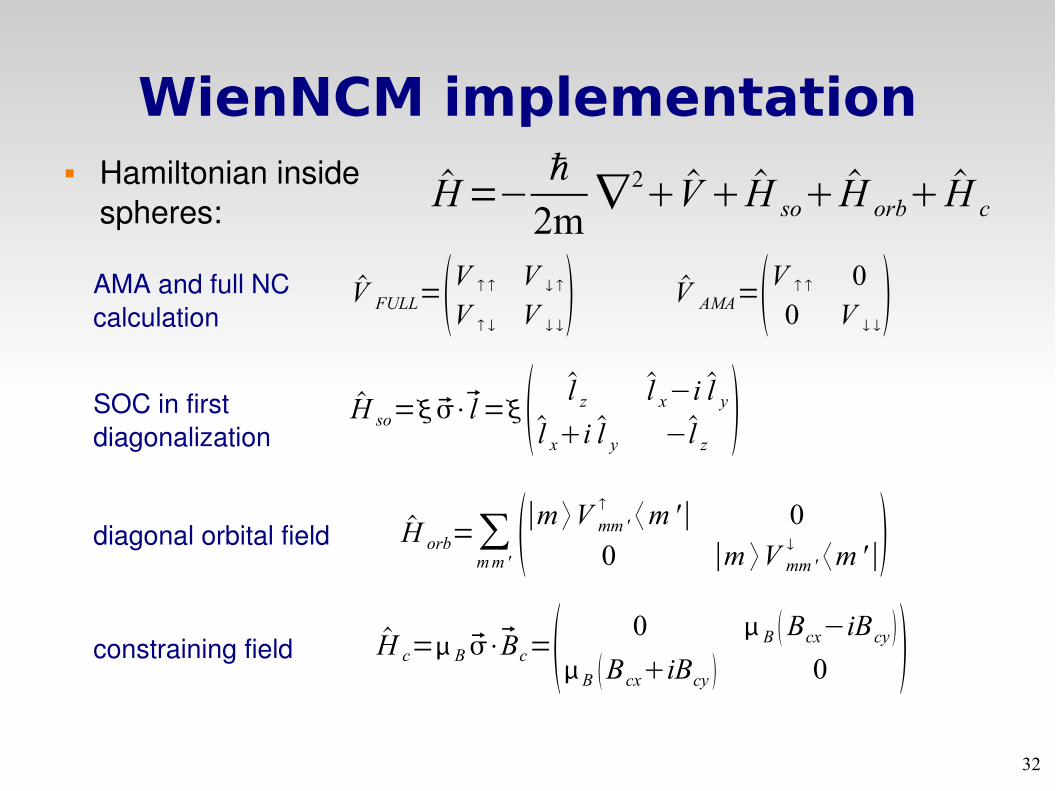
WienNCM implementation Hamiltonian inside 

spheres:H=−

ℏ

2m∇2 V H so H orb H c

AMA and full NC calculation

V FULL=V V

V V V AMA=V 0

0 V

SOC in first diagonalization

diagonal orbital field

constraining field

H so=⋅l= l z l x−i l yl xi l y −l z

H orb=∑mm '

∣m ⟩V mm' ⟨m'∣ 0

0 ∣m ⟩V mm'⟨m'∣

H c= B ⋅Bc= 0 B Bcx−iBcy B BcxiBcy 0

33

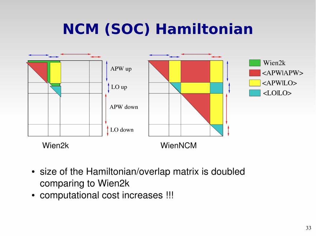
NCM (SOC) Hamiltonian

● size of the Hamiltonian/overlap matrix is doubled comparing to Wien2k

● computational cost increases !!!

Wien2k WienNCM

34

WienNCM – spin spirals

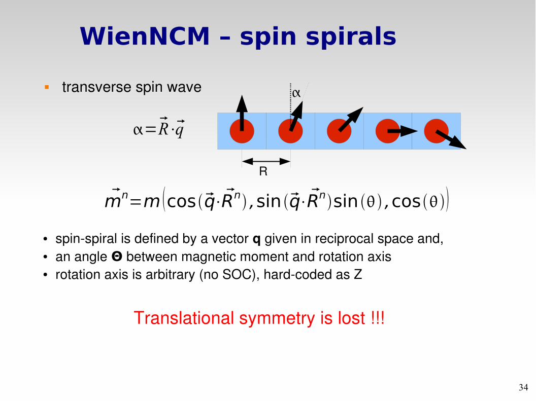
transverse spin wave

R

=R⋅q

mn=m cos q⋅Rn ,sin q⋅Rnsin ,cos

● spin­spiral is defined by a vector q given in reciprocal space and,● an angle Θ between magnetic moment and rotation axis ● rotation axis is arbitrary (no SOC), hard­coded as Z 

Translational symmetry is lost !!!

35

WienNCM – spin spirals

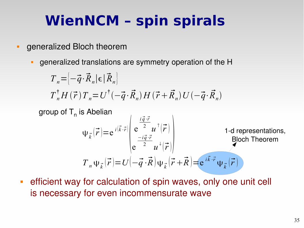
generalized Bloch theorem

generalized translations are symmetry operation of the H

T n={−q⋅Rn∣∣Rn }

T n k r =U −q⋅R k rR =e i k⋅r k r

k r =ei k⋅r e

i q⋅r2 u r

e−i q⋅r2 u r

efficient way for calculation of spin waves, only one unit cell is necessary for even incommensurate wave 

group of Tn is Abelian

T n†H r T n=U

†−q⋅RnH r RnU −q⋅Rn

1­d representations, Bloch Theorem

36

Usage● generate atomic and magnetic structure

1) create atomic structure2) create magnetic structure 

need to specify only directions of magnetic atomsuse utility programs: ncmsymmetry, polarangles, ...

● run initncm (initialization script)

● xncm ( WienNCM version of x script)

● runncm (WienNCM version of run script)

● find more in manual

runncm_lapw script:

xncm lapw0xncm lapw1xncm lapw2xncm lcorexncm mixer

37

WienNCM – case.inncm file

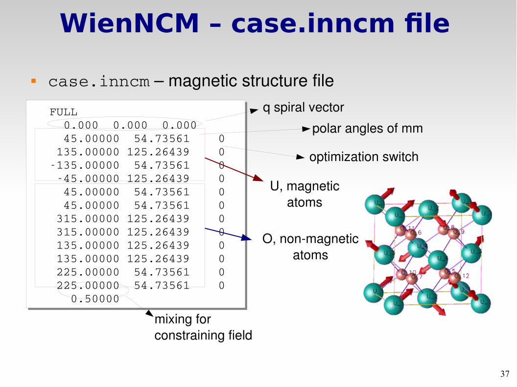
case.inncm – magnetic structure file

FULL                            0.000  0.000  0.000  45.00000  54.73561    0 135.00000 125.26439    0­135.00000  54.73561    0 ­45.00000 125.26439    0  45.00000  54.73561    0  45.00000  54.73561    0 315.00000 125.26439    0 315.00000 125.26439    0 135.00000 125.26439    0 135.00000 125.26439    0 225.00000  54.73561    0 225.00000  54.73561    0   0.50000

q spiral vector

polar angles of mm

optimization switch

mixing for constraining field

U, magnetic atoms

O, non­magnetic atoms