2 1 Introd ction2.1 Introductioncc.ee.ntu.edu.tw/~wujsh/9802PC/Chapter2_990408.pdf · 2 1 Introd...
107
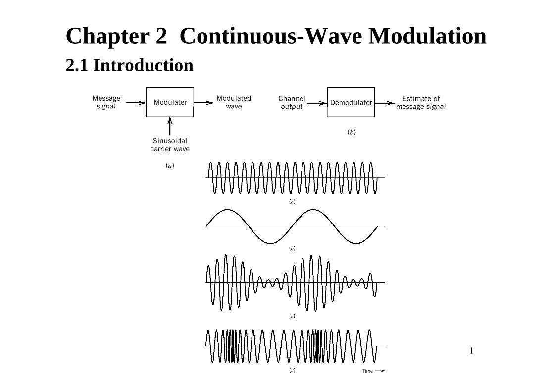
Chapter 2 Continuous-Wave Modulation 2 1 Introd ction 2.1 Introduction 1
Transcript of 2 1 Introd ction2.1 Introductioncc.ee.ntu.edu.tw/~wujsh/9802PC/Chapter2_990408.pdf · 2 1 Introd...
Chapter 2 Continuous-Wave Modulation2 1 Introd ction2.1 Introduction
1
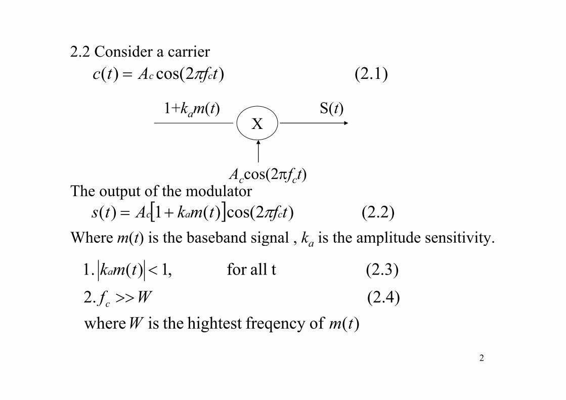
2.2 Consider a carrier (2.1) )2cos()( tfAtc cc π=
1+k m(t) S(t)X
1+kam(t) S(t)
The output of the modulator Accos(2πfct)
Where m(t) is the baseband signal , ka is the amplitude sensitivity. [ ] (2.2) )2cos()(1)( tftmkAts cac π+=
( ) g a p y
(2 4)2(2.3) t allfor ,1 )( .1
ftmka <
)( offreqency hightest theis where(2.4) .2
tmWWfc >>
2
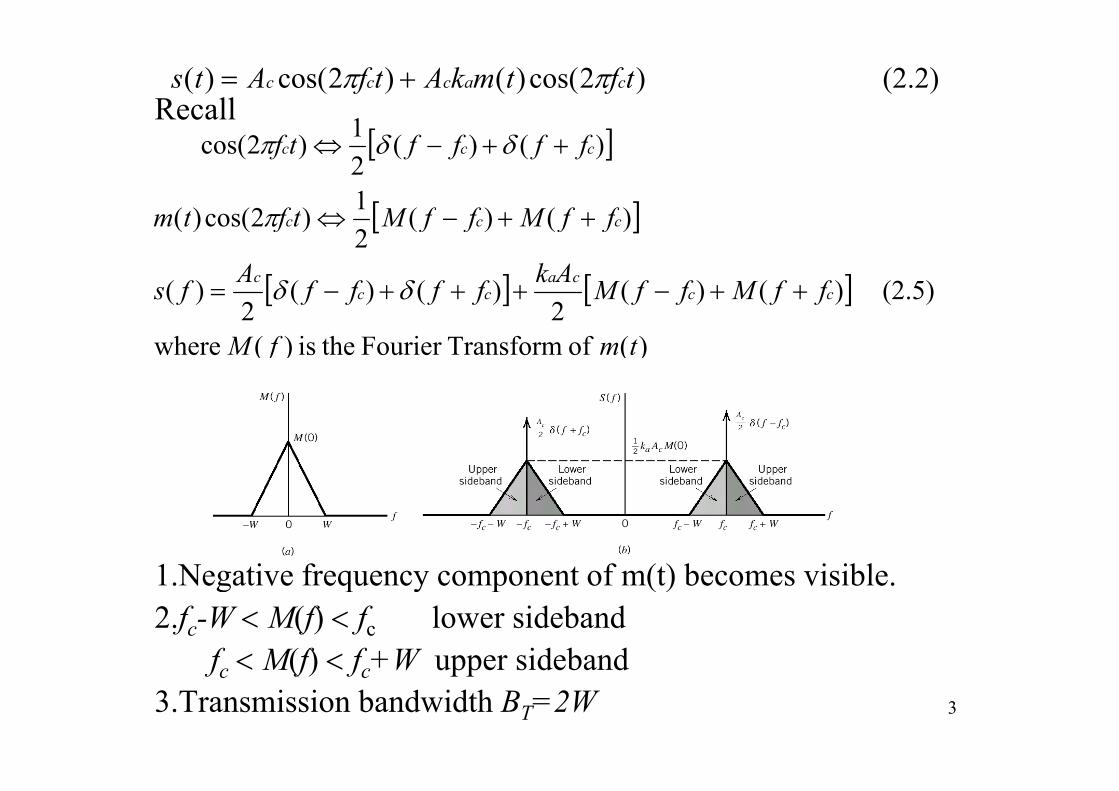
Recall(2.2) )2cos()()2cos()( tftmkAtfAts caccc ππ +=
1 [ ]
[ ])()(1)2cos()(
)()(21)2cos(
ffMffMtftm
fffftf ccc
++⇔
++−⇔
π
δδπ
[ ]
[ ] [ ] (2.5) )()(2
)()(2
)(
)()(2
)2cos()(
ffMffMAkffffAfs
ffMffMtftm
ccca
ccc
ccc
++−+++−=
++−⇔
δδ
π
[ ] [ ])( of Transform Fourier theis )( where
22tmfM
1 Negative frequency component of m(t) becomes visible1.Negative frequency component of m(t) becomes visible.2.fc-W < M(f) < fc lower sideband
f < M(f) < f +W upper sideband3
fc < M(f) < fc+W upper sideband3.Transmission bandwidth BT=2W
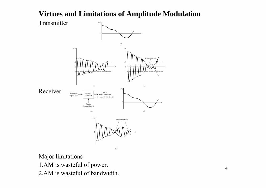
Virtues and Limitations of Amplitude ModulationTransmitter
Receiver
Major limitations
4
Major limitations 1.AM is wasteful of power.2.AM is wasteful of bandwidth.
2 3 Linear Modulation Schemes2.3 Linear Modulation Schemes
Linear modulation is defined by
(2.7) )2sin()()2cos()()( −= tftstftsts cQcI ππ
componentQuadrature)(component phase-In)(
==
tsts
Q
I
Three types of linear modulation:
componentQuadrature)(tsQ
1.Double sideband-suppressed carrier (DSB-SC) modulation2 Single sideband (SSB) modulation2.Single sideband (SSB) modulation3.Vestigial sideband (VSB) modulation
5
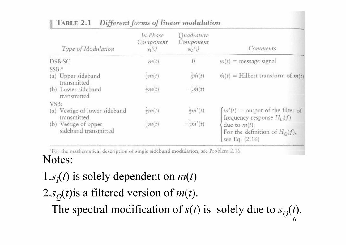
Notes:1 sI(t) is solely dependent on m(t)1.sI(t) is solely dependent on m(t)2.sQ(t)is a filtered version of m(t).
Th l difi i f ( ) i l l d ( )6
The spectral modification of s(t) is solely due to sQ(t).
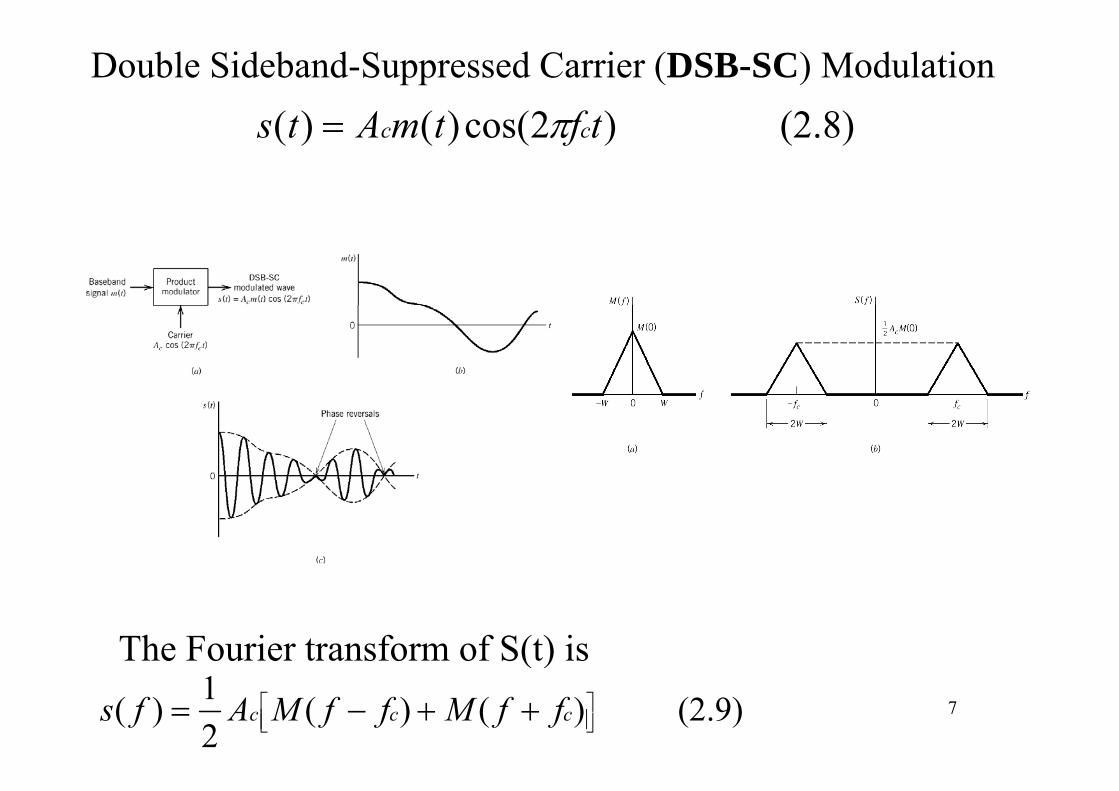
Double Sideband-Suppressed Carrier (DSB-SC) Modulation(2 8))2cos()()( tftmAts π= (2.8) )2cos()()( tftmAts cc π=
The Fourier transform of S(t) is 7
( )(2.9) )()(
21)( ⎥⎦
⎤⎢⎣⎡ ++−= ccc ffMffMAfs
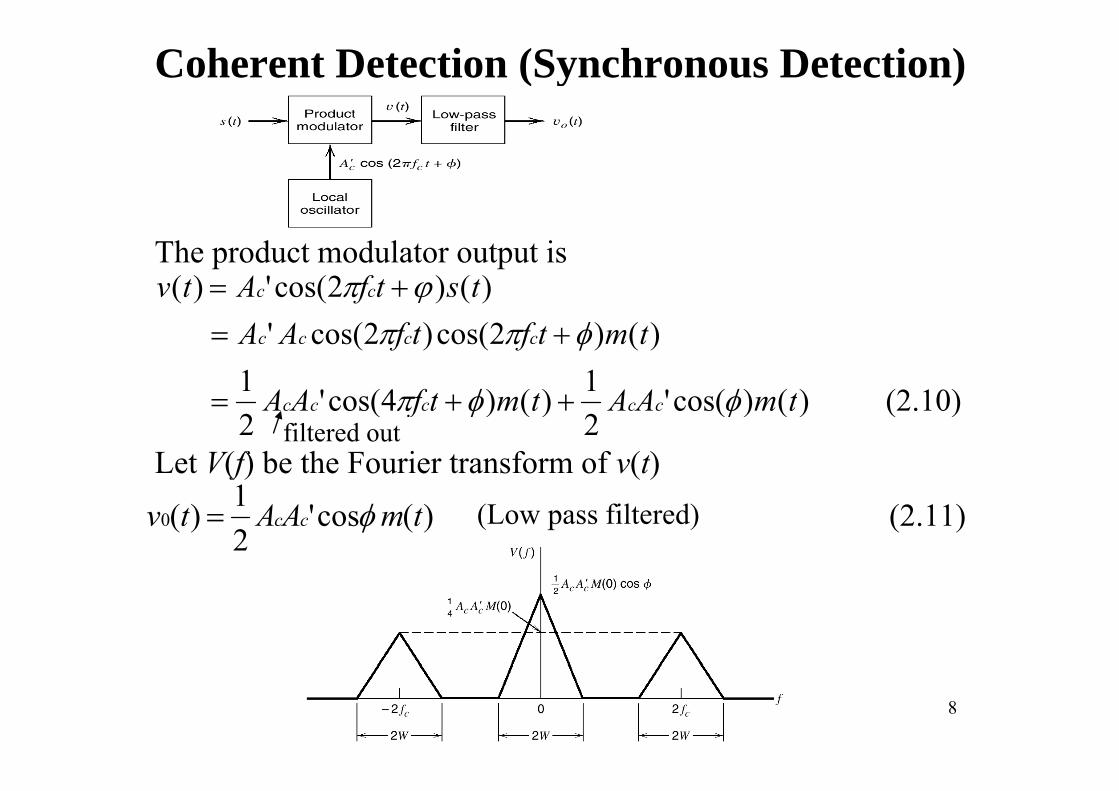
Coherent Detection (Synchronous Detection)
The product modulator output is )()2cos(' )( tstfAtv cc ϕπ +=
(2 10))()('1)()4('1)()2cos()2cos('
tAAttfAA
tmtftfAA cccc
φφ
φππ
++
+=
Let V(f) be the Fourier transform of v(t)
(2.10) )()cos('2
)()4cos('2
tmAAtmtfAA ccccc φφπ ++=
1
filtered out
(2.11) )( cos'21)(0 tmAAtv cc φ= (Low pass filtered)
8
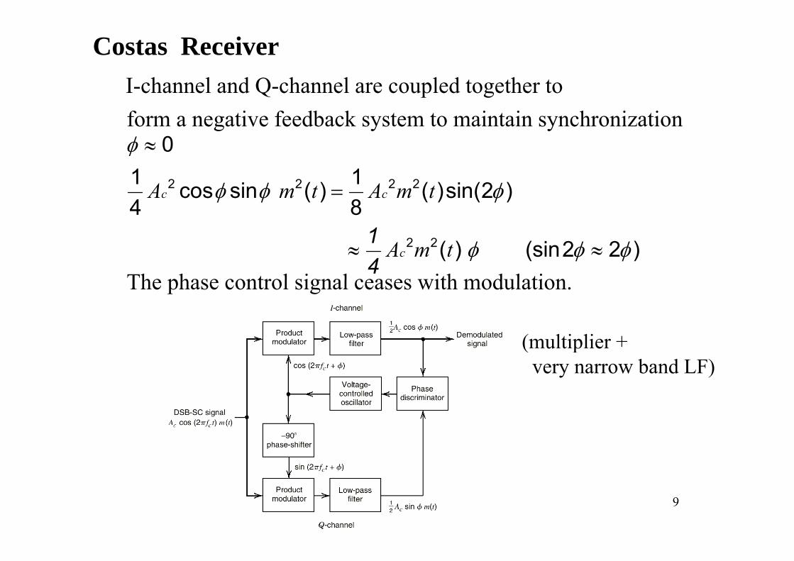
Costas ReceiverI-channel and Q-channel are coupled together toI channel and Q channel are coupled together to form a negative feedback system to maintain synchronization
0φ ≈
2 2 2 21 1cos sin ( ) ( )sin(2 )4 8
c cA m t A m t
φ
φ φ φ=
The phase control signal ceases with modulation
1 4
2 2( ) (sin2 2 )cA m t φ φ φ≈ ≈The phase control signal ceases with modulation.
(multiplier +(multiplier + very narrow band LF)
9
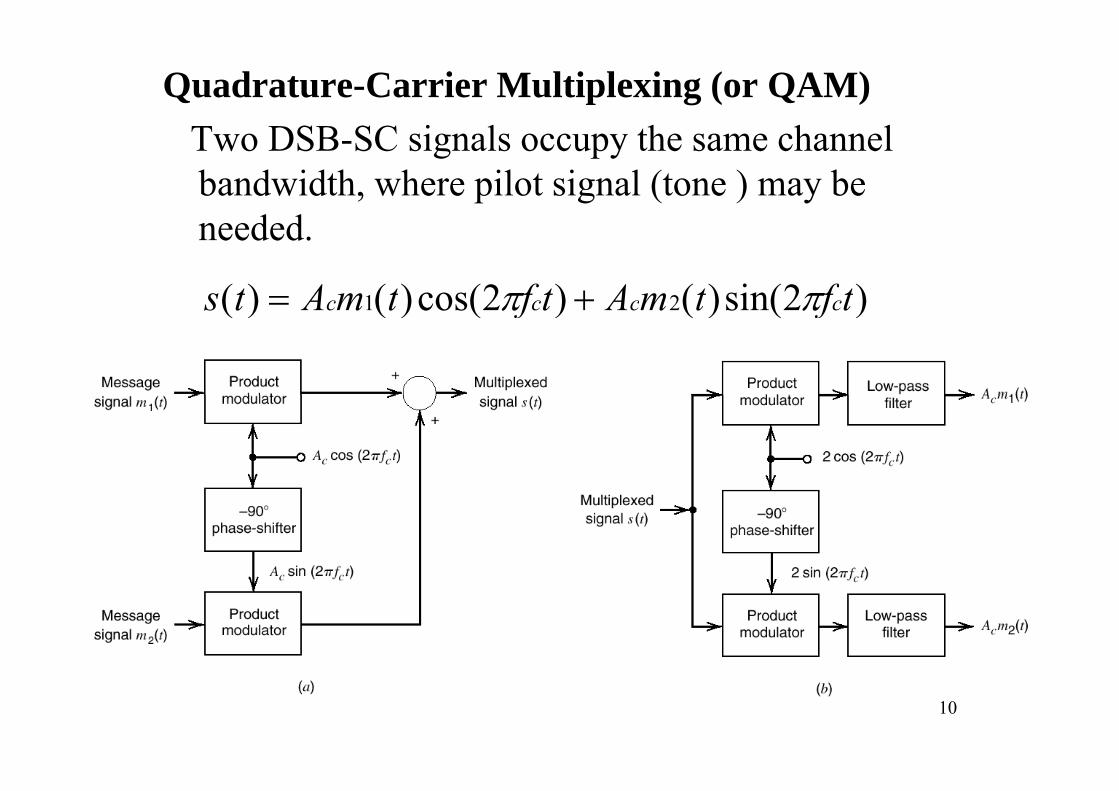
Quadrature-Carrier Multiplexing (or QAM)T DSB SC i l h h lTwo DSB-SC signals occupy the same channel bandwidth, where pilot signal (tone ) may be
d dneeded.
)2sin()()2cos()()( 21 tftmAtftmAts cccc ππ += )2sin()()2cos()()( 21 tftmAtftmAts cccc ππ +
10
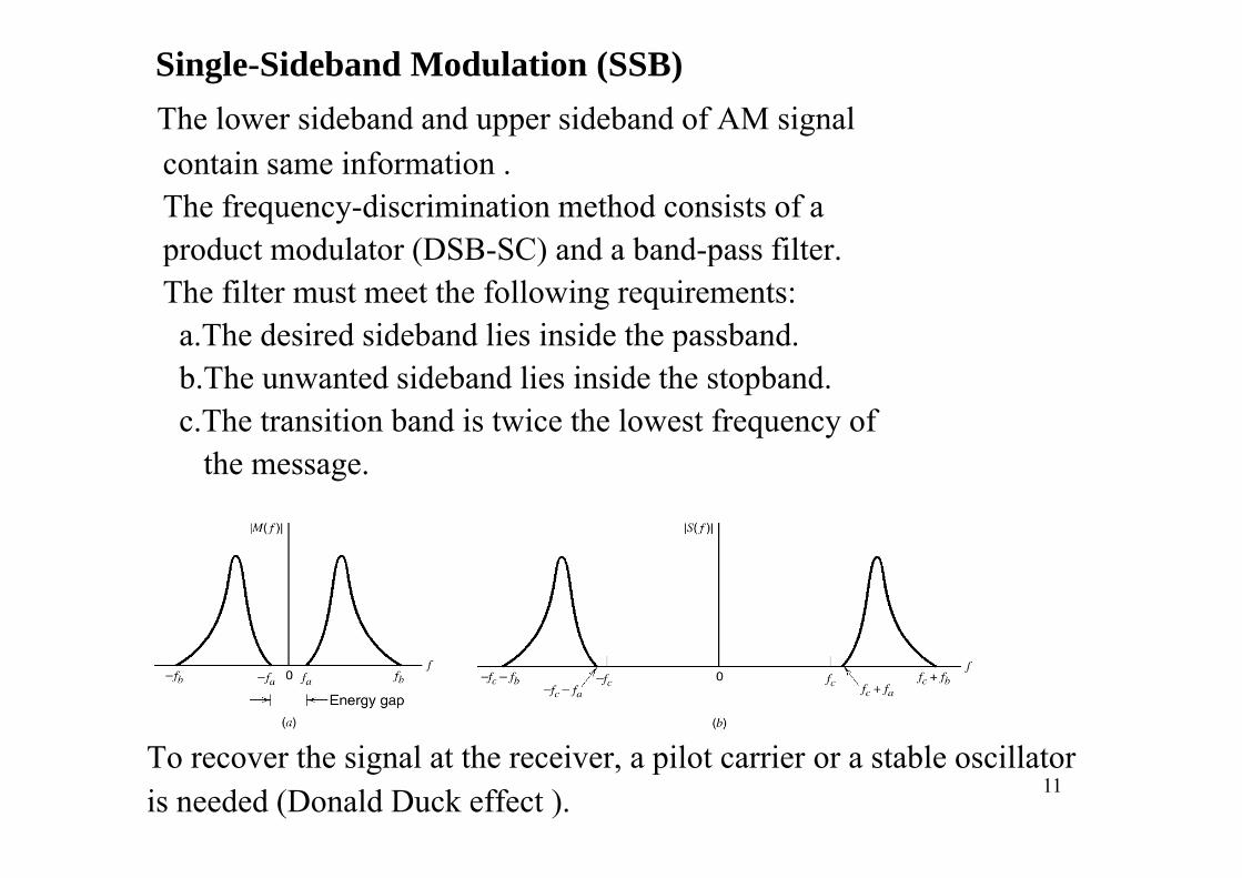
Single-Sideband Modulation (SSB)The lower sideband and upper sideband of AM signal contain same information .The frequency-discrimination method consists of a
d d l (DSB SC) d b d filproduct modulator (DSB-SC) and a band-pass filter.The filter must meet the following requirements:a The desired sideband lies inside the passbanda.The desired sideband lies inside the passband.b.The unwanted sideband lies inside the stopband. c.The transition band is twice the lowest frequency of
the message.
11To recover the signal at the receiver, a pilot carrier or a stable oscillator is needed (Donald Duck effect ).
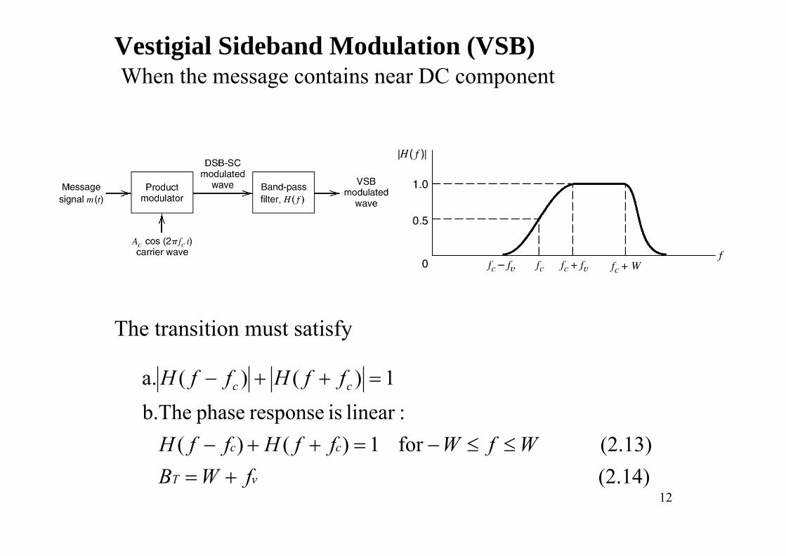
Vestigial Sideband Modulation (VSB)When the message contains near DC component
The transition must satisfy
liihb h 1)()(.a ffHffH cc =++−
(2.13) for 1)()( :linearisresponsephase b.The
W fWffHffH cc ≤≤−=++−
12(2.14) fWB νT +=
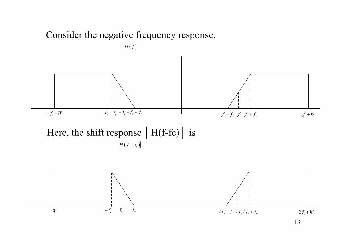
Consider the negative frequency response:g q y p( )H f
c vf f− cf c vf f+ cf W+c vf f− +cf−c vf f− −cf W− −
Here, the shift response │H(f-fc)│ is( )cH f f−
f0 2 c vf f− 2 cf 2 c vf f+ 2 cf W+vf0vf−W
13
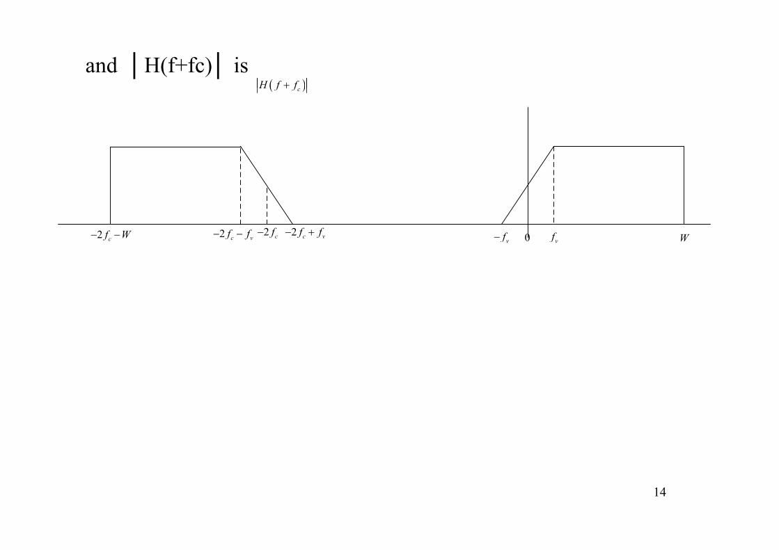
and │H(f+fc)│ is( )H f f+( )cH f f+
vf− 0 vf W2 c vf f− +2 cf−2 c vf f− −2 cf W− −
14
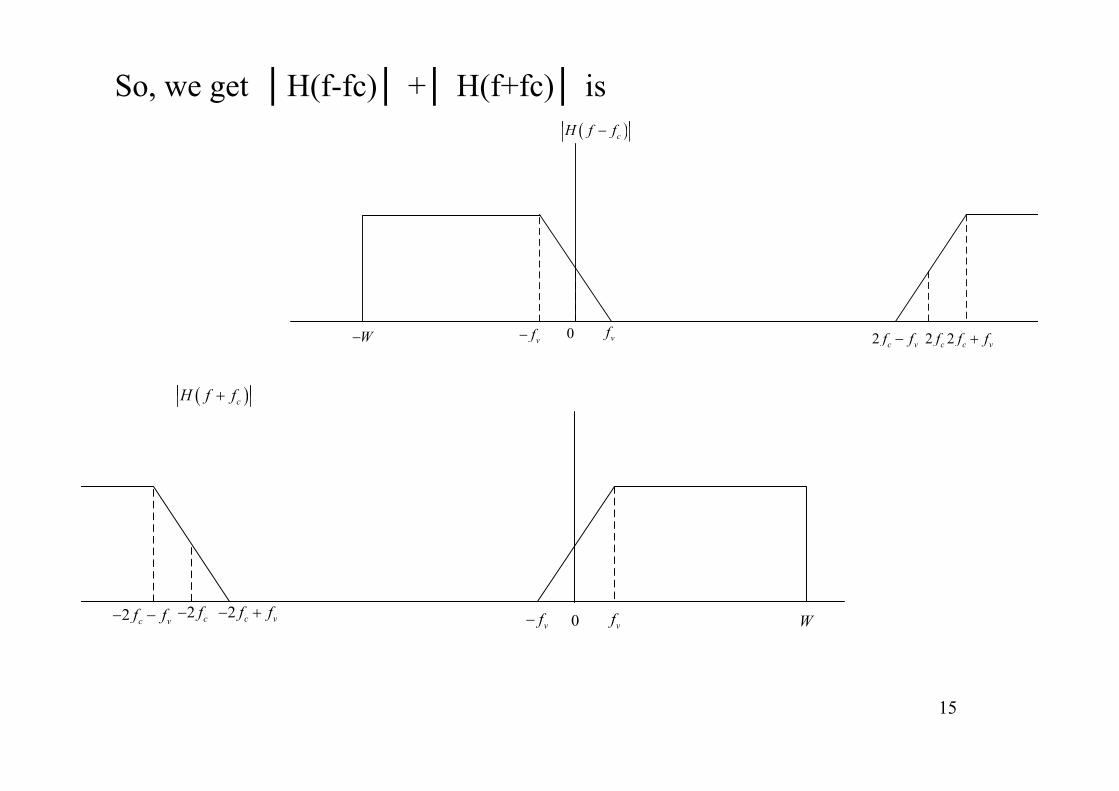
So, we get │H(f-fc)│ +│ H(f+fc)│ is( )H f f( )cH f f−
2 c vf f− 2 cf 2 c vf f+vf0vf−W−
( )H f f+( )cH f f+
vf− 0 vf W2 c vf f− +2 cf−2 c vf f− −
15
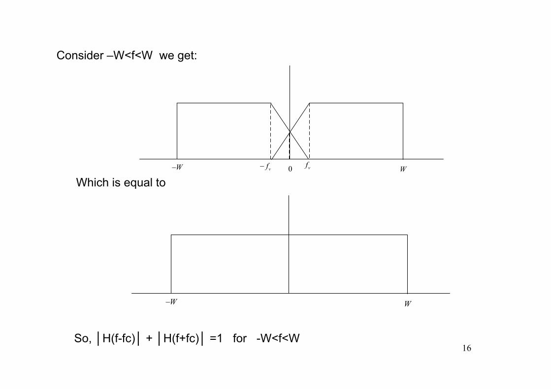
Consider –W<f<W we get:
vfvf−W− 0 W
Which is equal to
W− W
So, │H(f-fc)│ + │H(f+fc)│ =1 for -W<f<W16
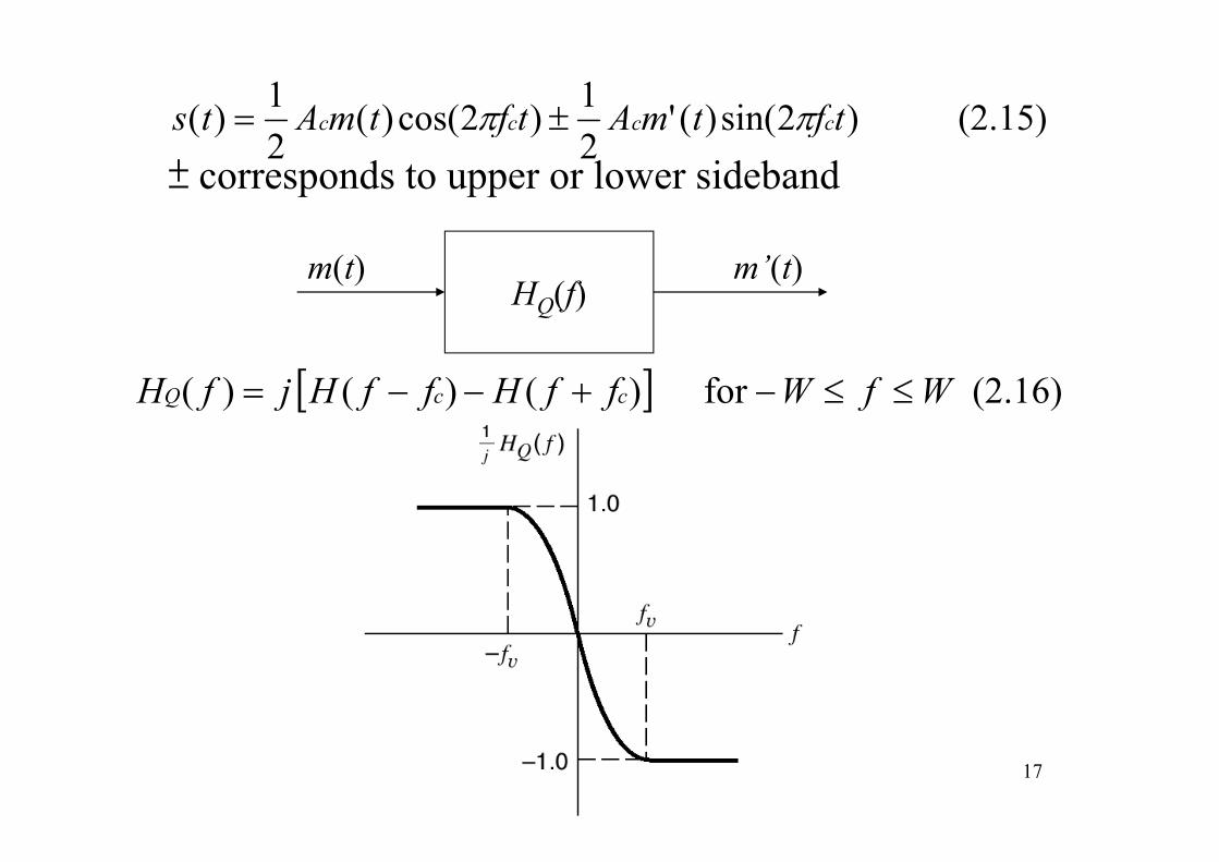
(2.15) )2sin()('21)2cos()(
21)( tftmAtftmAts cccc ππ ±=
± corresponds to upper or lower sideband22
ff
HQ(f)m(t) m’(t)
[ ] (2.16) for )()( )( W f WffHffHjfH ccQ ≤≤−+−−=
17
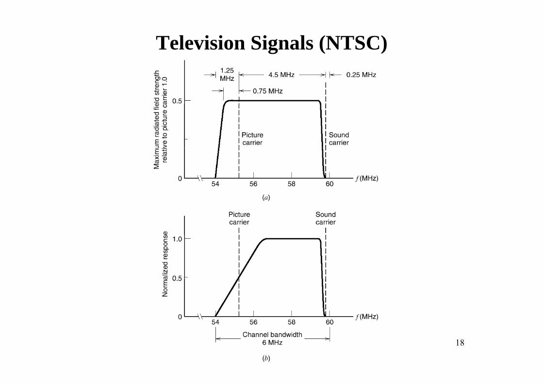
Television Signals (NTSC)
18
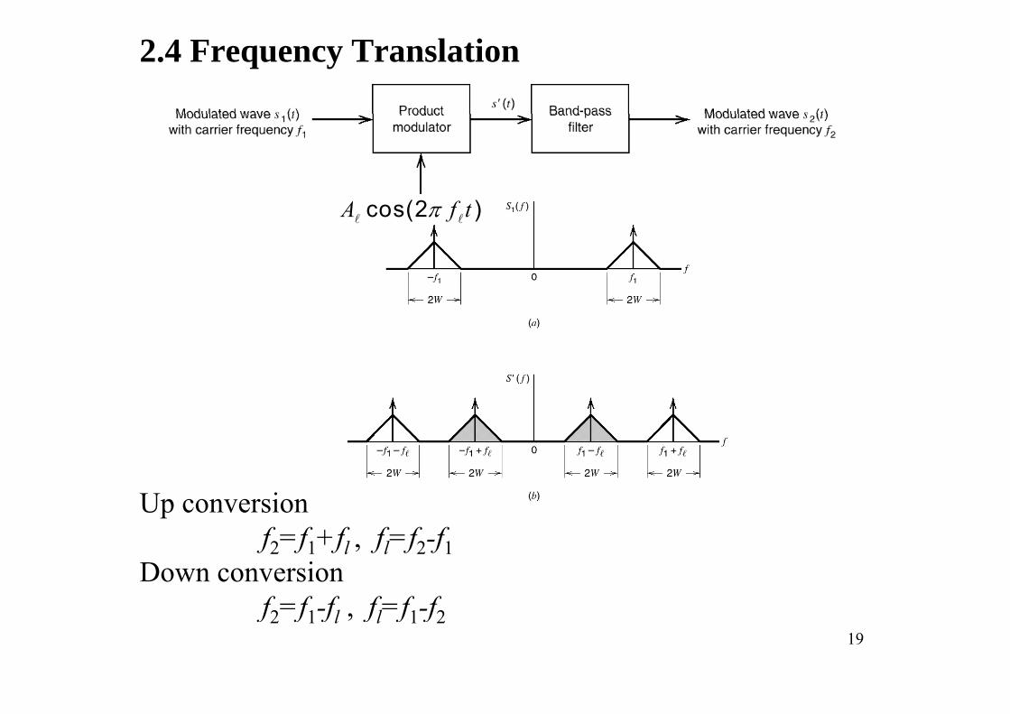
2.4 Frequency Translation
cos(2 )A f tπl l
Up conversionf2=f1+fl , fl=f2-f1
Down conversionf f f f f f
19
f2=f1-fl , fl=f1-f2
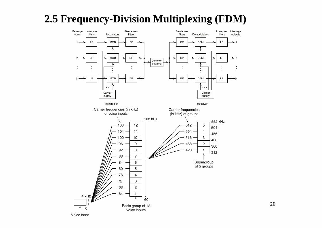
2.5 Frequency-Division Multiplexing (FDM)
20
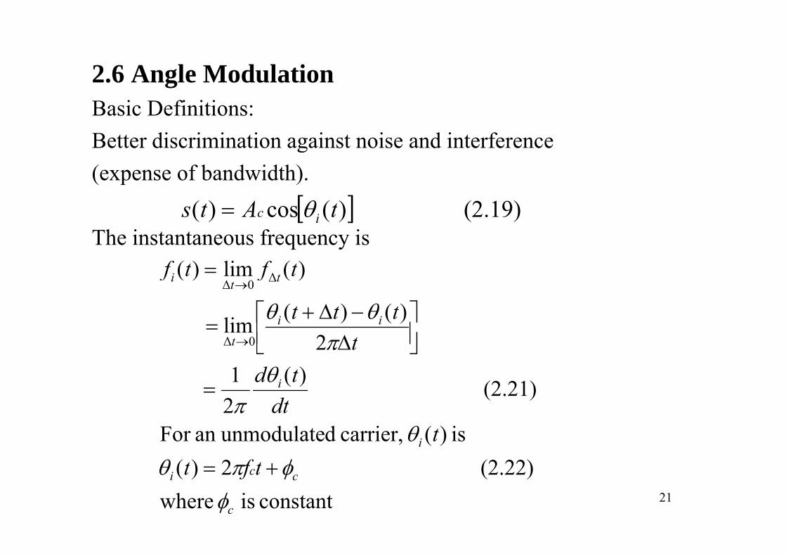
2.6 Angle ModulationBasic Definitions:Better discrimination against noise and interference g(expense of bandwidth).
[ ] (2.19))(cos)( tAts ic θ=The instantaneous frequency is
[ ] (2.19) )(cos)( tAts ic θ
)(lim)( Δti tftf =
2)()(lim
)()(
0Δ
Δ0Δ
ii
t
tti
tttt
ff
πθθ
⎥⎦⎤
⎢⎣⎡
Δ−Δ+
=→
→
(2.21) )(21
20Δ
i
t
dttd
tθ
π
π
=
⎥⎦⎢⎣ Δ→
(2 22)2)( is )( carrier, dunmodulate anFor
2i
tftt
dt
φπθθ
π
+=21constant is where
(2.22) 2)(
c
cci tftφ
φπθ +=
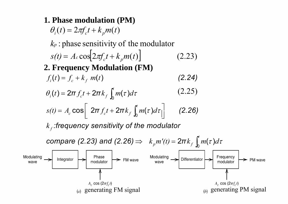
1. Phase modulation (PM))(2)( tmktft pci += πθ
[ ] (2 23))(2cosmodulator theofy sensitivit phase :
)()(
tmktfAs(t)k
fp
pci
+= π
πθ
2. Frequency Modulation (FM)[ ] (2.23) )(2cos tmktfAs(t) pcc += π
(2 24)( ) ( )f t f k m t= + (2.24)
π π0
( ) ( )
( ) 2 2 ( )
i c f
t
i c f
f t f k m t
t f t k m dθ τ τ
= +
= + ∫ (2.25)
π π (2.26)
:frequency sensitivity of the modulator0
cos 2 2 ( )t
c c fs(t) A f t k m d
k
τ τ⎡ ⎤= +⎢ ⎥⎣ ⎦∫:frequency sensitivity of the modulator
compare (2.23) and (2.26)
f
p
k
k m'⇒ π0
2 ( )t
f(t) k m dτ τ= ∫
22generating FM signal generating PM signal
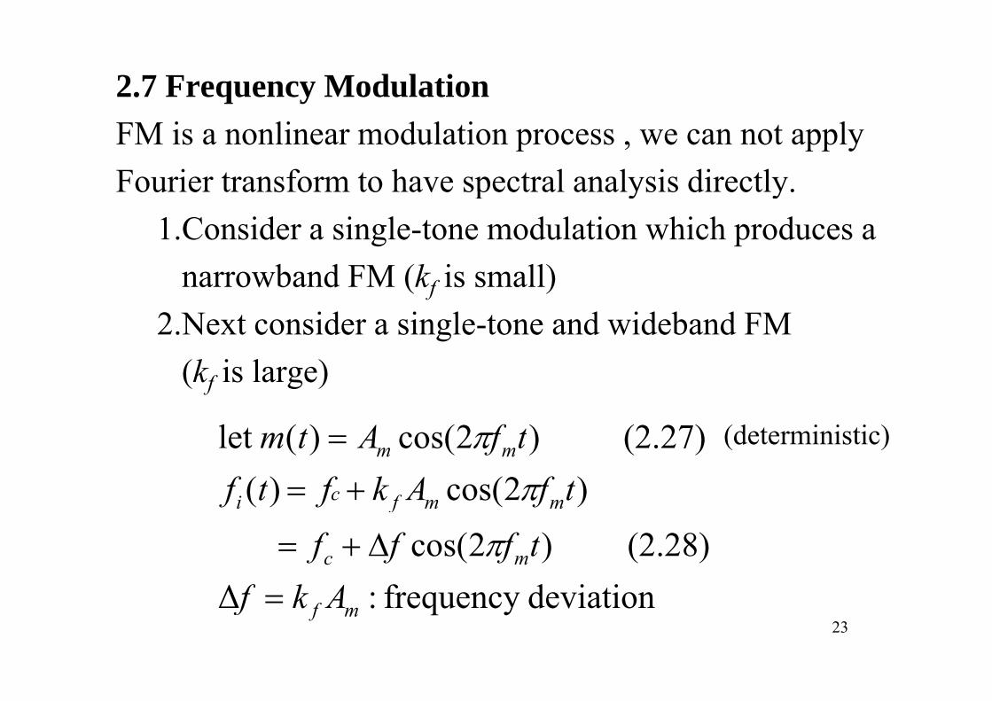
2.7 Frequency ModulationFM is a nonlinear modulation process , we can not apply Fourier transform to have spectral analysis directly.Fourier transform to have spectral analysis directly.
1.Consider a single-tone modulation which produces a b d FM (k i ll)narrowband FM (kf is small)
2.Next consider a single-tone and wideband FM (kf is large)
(2 27))2()(l t tfAt (d t i i ti )
)2cos( )((2.27) )2cos()(let
mmfci
mm
tfAkftftfAtm
+==
ππ (deterministic)
d i tifΔ(2.28) )2cos( mc
f
Akftfff Δ+= π
23 deviationfrequency :Δ mf Akf =
)(2)( (2.25), Recall0
ττπθ dftt
ii = ∫(2.30) )2sin(2 π tf
fftπf mc
Δ+=
(2.31) index Modulation β ffm
Δ=
(2.32) )2sin(2)(
( )
πβθ
β
tftπftf
mci
m
+=[ ]
dill hiFMN b d(2.33) )2sin(2cos)( ( ))()(
βπβπ
βtftfAts
ff
mcc
mi
+=(2.19) =>
radian. onenlarger thais, FM Widebandradian.one ansmaller this, FM Narrowband
ββ
24
gβ
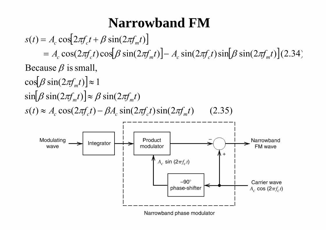
Narrowband FM[ ])2i (2)( ffA β[ ]
[ ] [ ] )34.2( )2sin(sin)2sin()2sin(cos)2cos( )2sin(2cos)(
tftfAtftfAtftfAts
mccmcc
mcc
πβππβππβπ
−=+=
[ ] 1)2sin(cossmall, isBecausetfmπβ
β≈
[ ](2.35) )2sin()2sin()2cos()(
)2sin()2sin(sintftfAtfAts
tftf
mcccc
mm
ππβππβπβ
−≈≈
( ))()()()( fff mcccc β
25
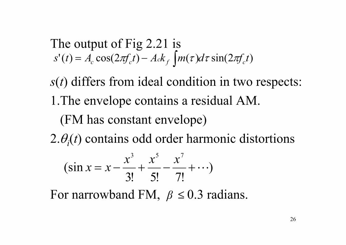
Th f Fi 2 21 iThe output of Fig 2.21 is )2sin()()2cos()(' tfdmkAtfAts cfccc πττπ ∫−=
s(t) differs from ideal condition in two respects:∫
1.The envelope contains a residual AM.(FM has constant envelope)(FM has constant envelope)
2.θi(t) contains odd order harmonic distortions
)!7!5!3
(sin753
L+−+−=xxxxx
For narrowband FM, ≤ 0.3 radians. !7!5!3
β
26
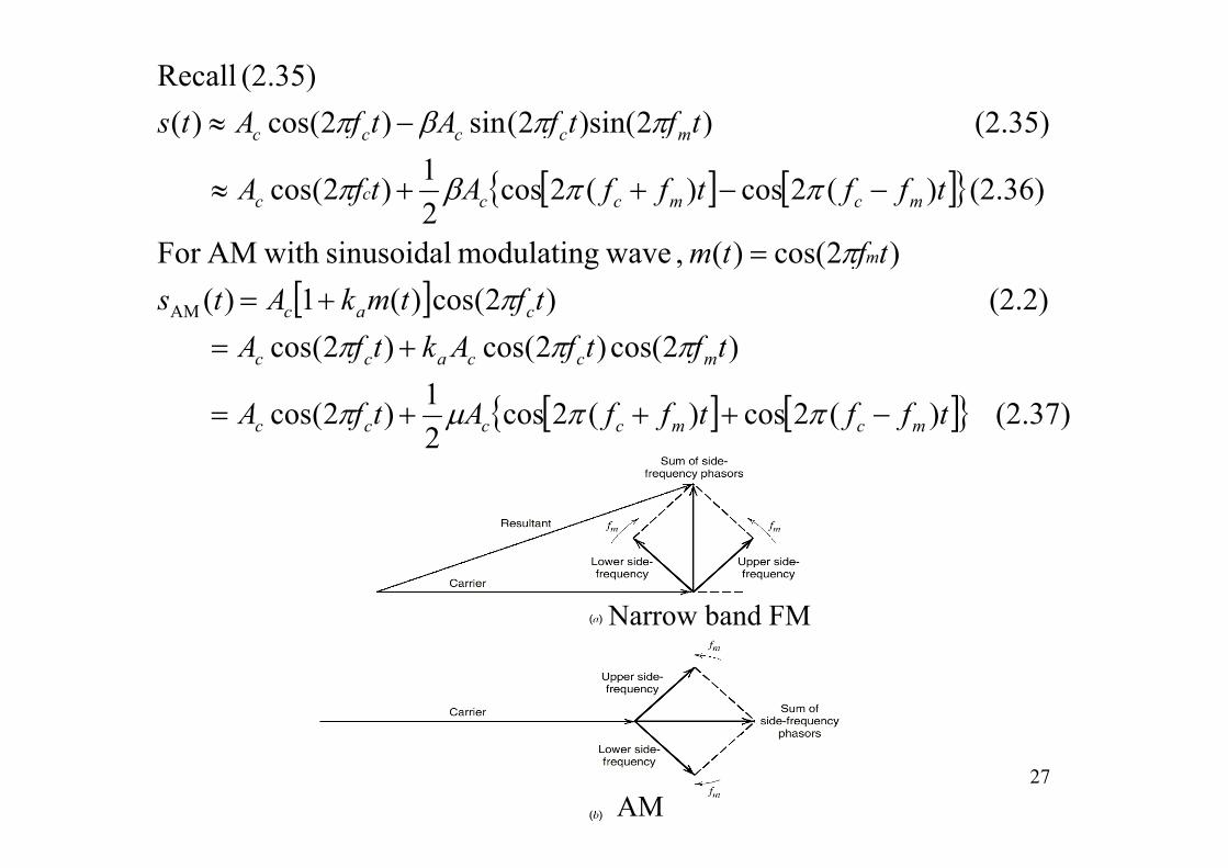
(2.35) )2)sin(2(sin)2(cos)((2.35)Recall
tftfAtfAts mcccc −≈ ππβπ
[ ] [ ]{ }(2.36) )(2cos)(2cos21)2(cos
( ))) (()()(
tfftffAtfA
fff
mcmcccc
mcccc
−−++≈ ππβπ
β
[ ])()()(
(2.2) )2(cos)(1 )()2cos()( ,wavemodulatingsinusoidal with AMFor
AM
ffkftftmkAts
tftm
cac
m
+==
ππ
[ ] [ ]{ } (2.37) )(2cos)(2cos21)2(cos
)2cos()2(cos)2(cos
tfftffAtfA
tftfAktfA
mcmcccc
mccacc
−+++=
+=
ππμπ
πππ
2
Narrow band FM
27AM
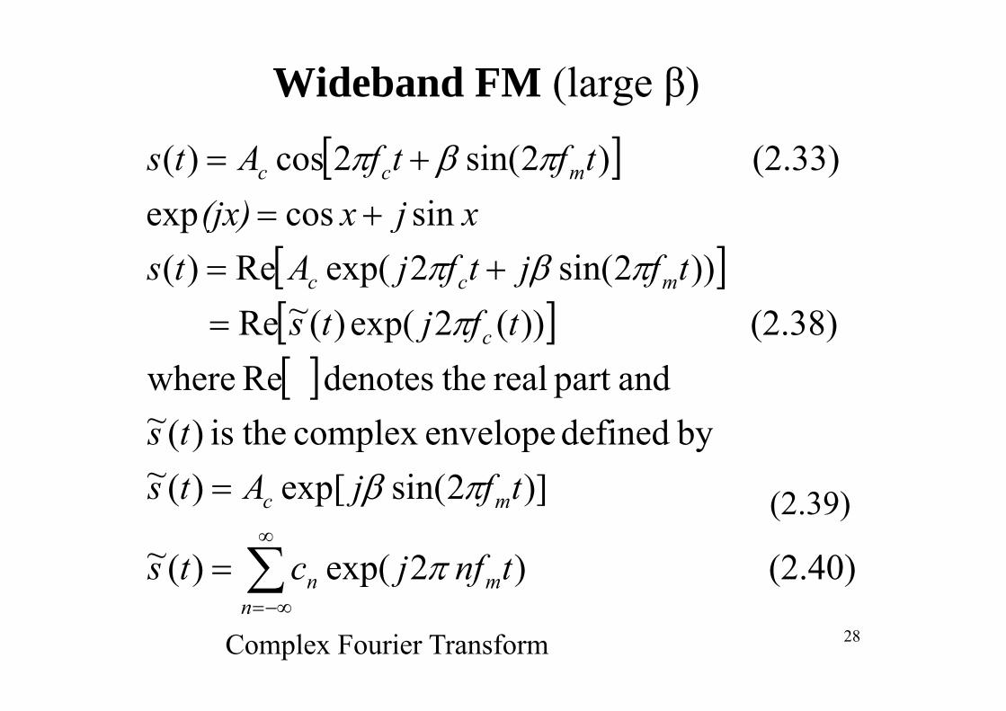
Wideband FM (large β)
[ ] (2.33) )2sin(2cos)( += mcc tftfAts πβπ
[ ]))2sin(2exp(Re)(sincosexp
+=+=
tfjtfjAtsxjx(jx)
πβπ[ ][ ] (2.38) ))(2exp()(~Re
))2sin(2exp(Re)(=
+
c
mcc
tfjtstfjtfjAts
ππβπ
[ ]bydefinedenvelopecomplextheis)(~ andpart real thedenotes Re where
ts)]2sin(exp[)(~
bydefined envelopecomplex theis)(= mc tfjAts
tsπβ (2.39)
(2.40) )2exp()(~ ∑∞
= mn t nfjcts π
( )
28
−∞=n
Complex Fourier Transform
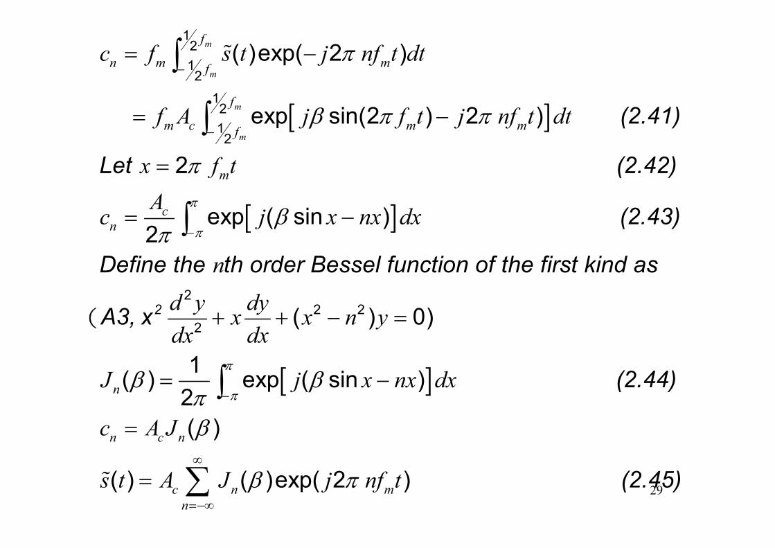
1212
( )exp( 2 )m
m
f
n m mfc f s t j nf t dtπ
−= −∫ %
[ ] (2.41)1212
exp sin(2 ) 2 )m
m
f
m c m mff A j f t j nf t dtβ π π
−= −∫
[ ]
Let (2.42)2
( i )
m
c
x f tA j d
π
β
=
(2 43)π
∫ [ ] exp ( sin )2
cnc j x nx dxβ
π= − (2.43)
Define the th order Bessel function of the first kind asnπ−∫
2A3, x2
2 22 ( ) 0)d y dyx x n y
dx dx+ + − =(
[ ] (2.44)1( ) exp ( sin )2n
dx dx
J j x nx dxπ
πβ β
π −= −∫2
( )n c nc A Jππ
β=
∫
∞
29( ) ( )c nn
s t A J β=−
=% (2.45)exp( 2 )mj nf tπ∞
∞∑
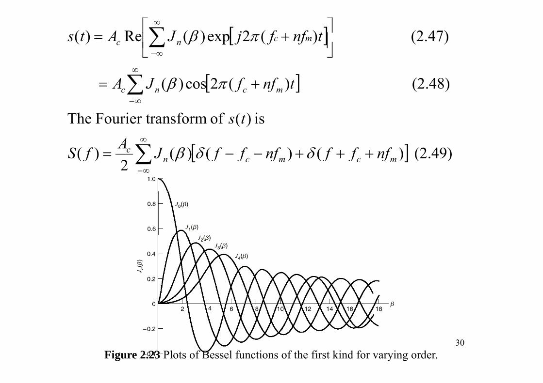
[ ] (2.47) )(2exp)(Re)( mcnc tnffjJAts ⎥⎦
⎤⎢⎣
⎡ += ∑∞
∞−
πβ
[ ] (2.48) )(2cos)( mcnc tnffJA += ∑∞
∞−
πβ
[ ] (2 49))()()()(
is )( of ransform Fourier tThe
ffffffJAfS
ts
∑∞
δδβ [ ] (2.49) )()()(2
)( mcmcnc nfffnfffJAfS +++−−= ∑
∞−
δδβ
30Figure 2.23 Plots of Bessel functions of the first kind for varying order.
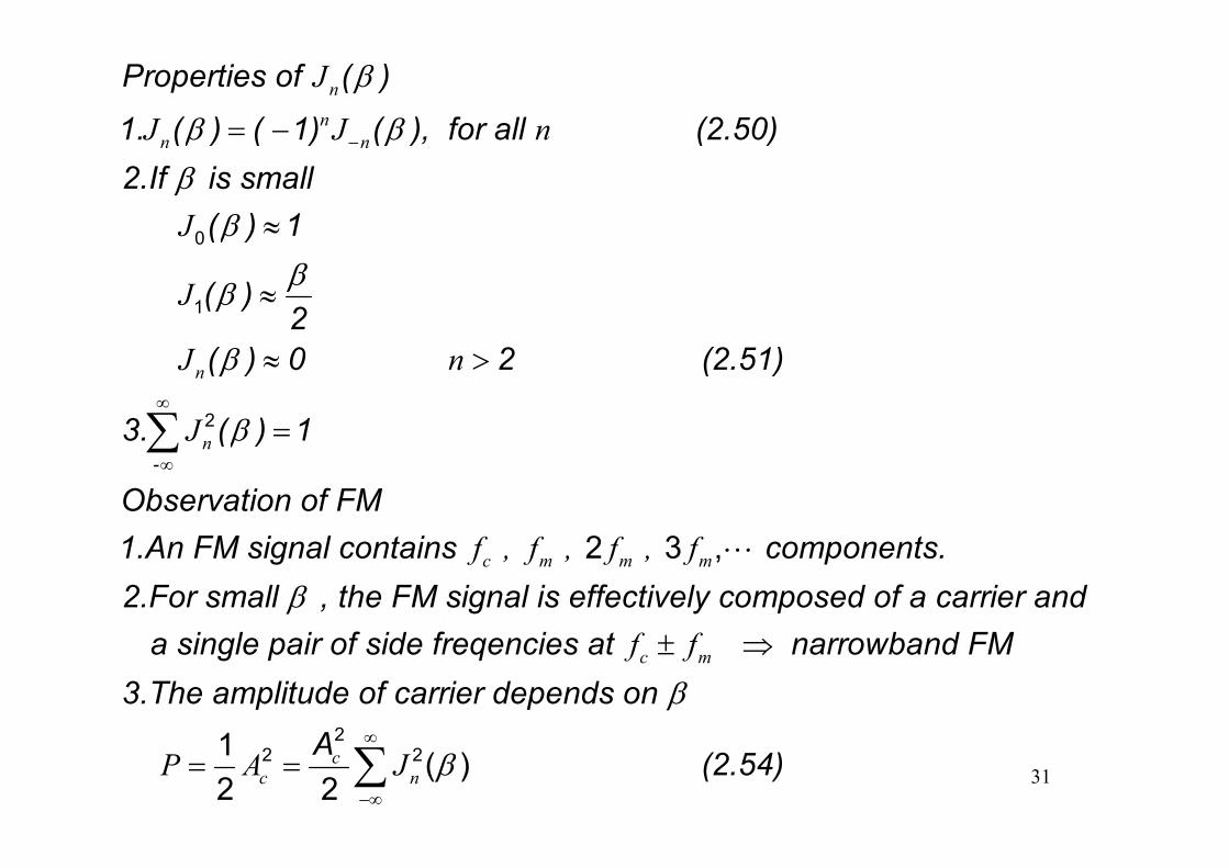
Properties of ( )
1. ( ) ( 1) ( ), for all (2.50)n
n
J
J J n
β
β β= −1. ( ) ( 1) ( ), for all (2.50)2.If is small ( ) 10
n nJ J n
J
β ββ
β
−
≈( )
( )2
0
1J
βββ ≈
( ) 0 2 (2.51)
3 ( ) 12
nJ n
J
β
β∞
≈ >
=∑-
3. ( ) 1
Observation o
nJ β∞
=∑f FM
1.An FM signal contains components.2.For small , the FM signal is effectively composed of a carrier and
2 3 ,c m m mf , f , f , fβ
L
a single pair of side freqencies at narrowband FM3.The am
c mf f± ⇒
plitude of carrier depends on 2
β
31A (2.54)
22 21 ( )
2 2c
c nP A J β∞
−∞
= = ∑
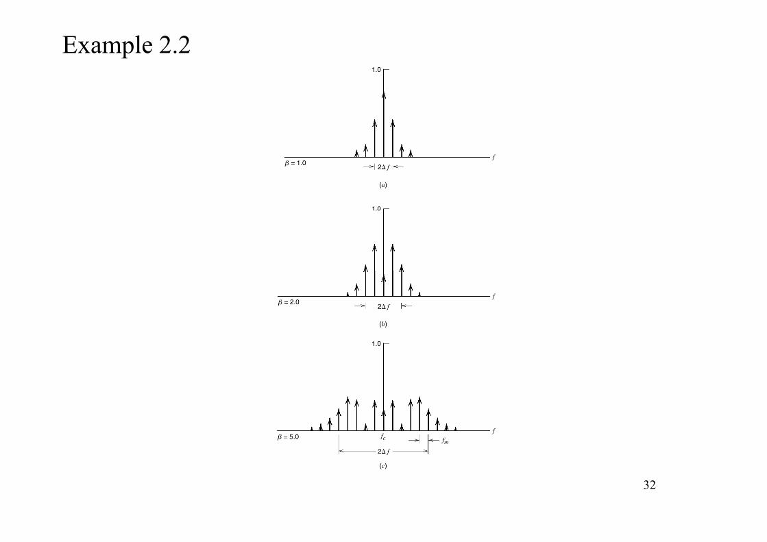
Example 2.2
32
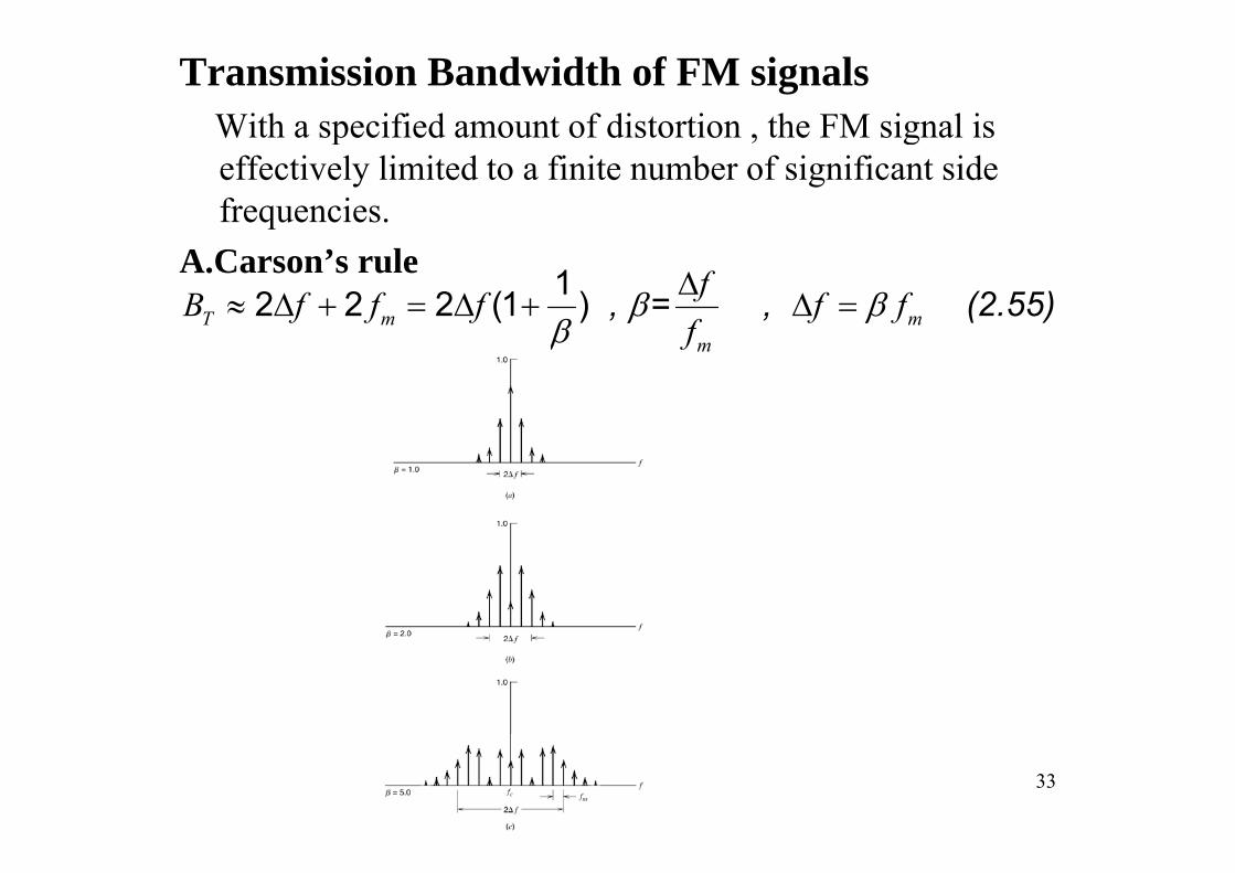
Transmission Bandwidth of FM signalsWith a specified amount of distortion , the FM signal is p , geffectively limited to a finite number of significant side frequencies.
A.Carson’s rule , = , (2.55)12 2 2 (1 )T m m
fB f f f f ff
β ββ
Δ≈ Δ + = Δ + Δ =
mfβ
33
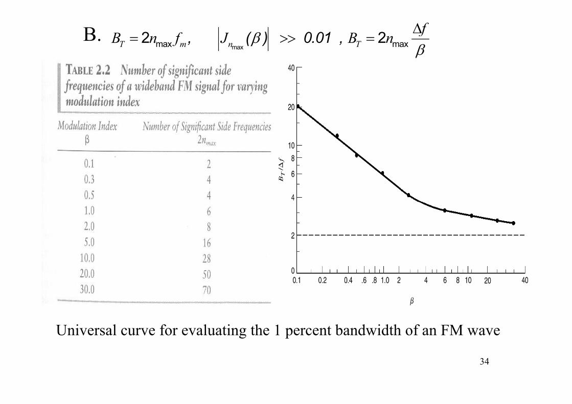
B. , ( ) 0.01 , maxmax max2 2T m n T
fB n f J B nββΔ
= >> =
Universal curve for evaluating the 1 percent bandwidth of an FM wave
34
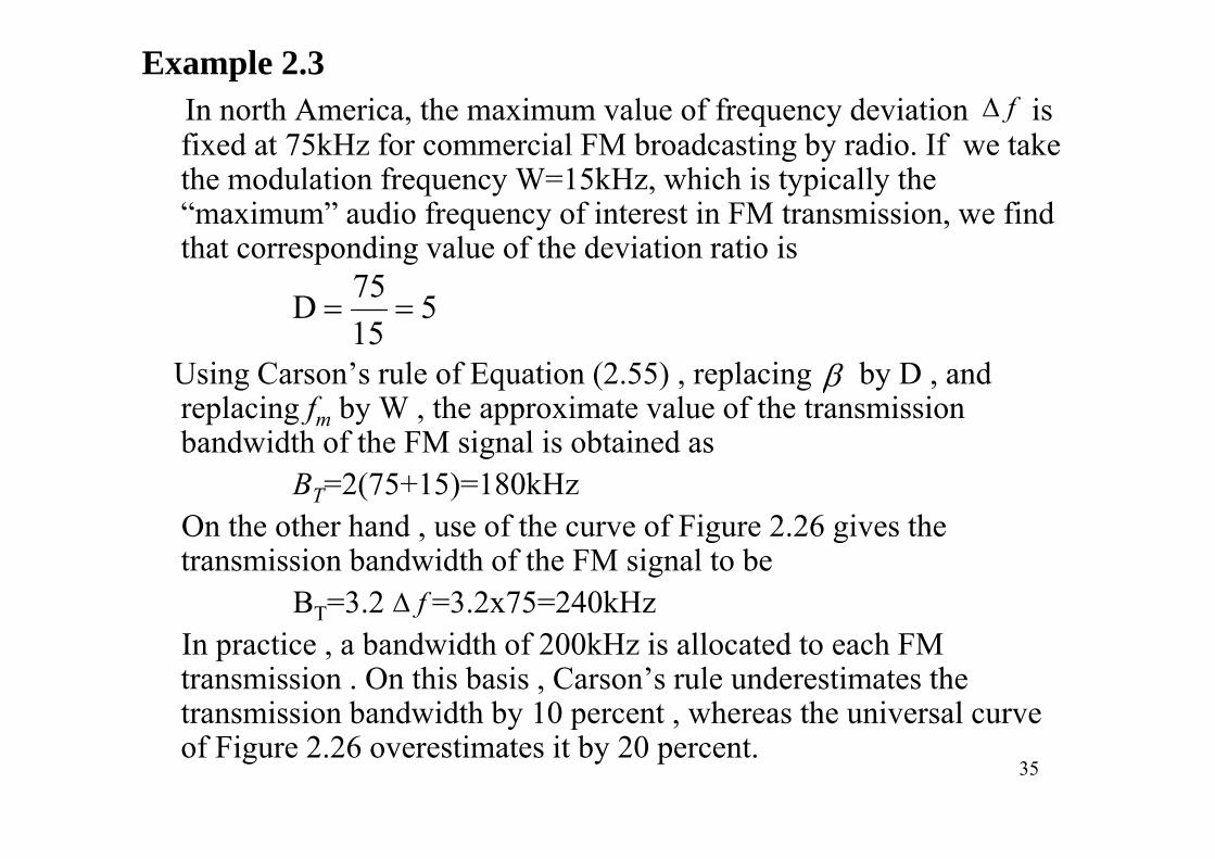
Example 2.3In north America, the maximum value of frequency deviation is fi d t 75kH f i l FM b d ti b di If t k
fΔfixed at 75kHz for commercial FM broadcasting by radio. If we take the modulation frequency W=15kHz, which is typically the “maximum” audio frequency of interest in FM transmission, we find that corresponding value of the deviation ratio is
51575D ==
Using Carson’s rule of Equation (2.55) , replacing by D , and replacing fm by W , the approximate value of the transmission
15β
bandwidth of the FM signal is obtained asBT=2(75+15)=180kHz
On the other hand use of the curve of Figure 2 26 gives theOn the other hand , use of the curve of Figure 2.26 gives the transmission bandwidth of the FM signal to be
BT=3.2 =3.2x75=240kHzfΔIn practice , a bandwidth of 200kHz is allocated to each FM transmission . On this basis , Carson’s rule underestimates the transmission bandwidth by 10 percent , whereas the universal curve
35
transmission bandwidth by 10 percent , whereas the universal curve of Figure 2.26 overestimates it by 20 percent.
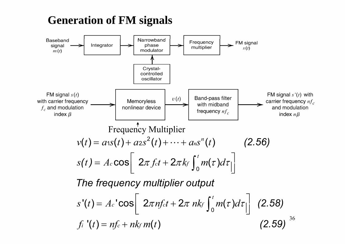
Generation of FM signals
(2.56)21 2( ) ( ) ( ) ( )n
nv t a s t a s t a s t= + + +L
Frequency Multiplier
( )
0cos 2 2 ( )
tc c fs t A f t k m dπ π τ τ⎡ ⎤= +⎢ ⎥⎣ ⎦∫
The frequency multiplier output
(2 58)'( ) 'cos 2 2 ( )t
c c fs t A nf t nk m dπ π τ τ⎡ ⎤= +⎢ ⎥⎣ ⎦∫36
(2.58)
0
( ) cos 2 2 ( )
'( ) ( )
c c f
i c f
s t A nf t nk m d
f t nf nk m t
π π τ τ+⎢ ⎥⎣ ⎦= +
∫ (2.59)
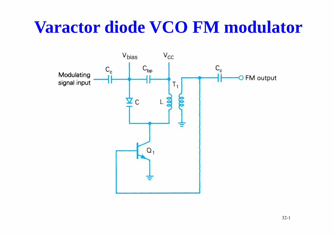
Varactor diode VCO FM modulator
32-1
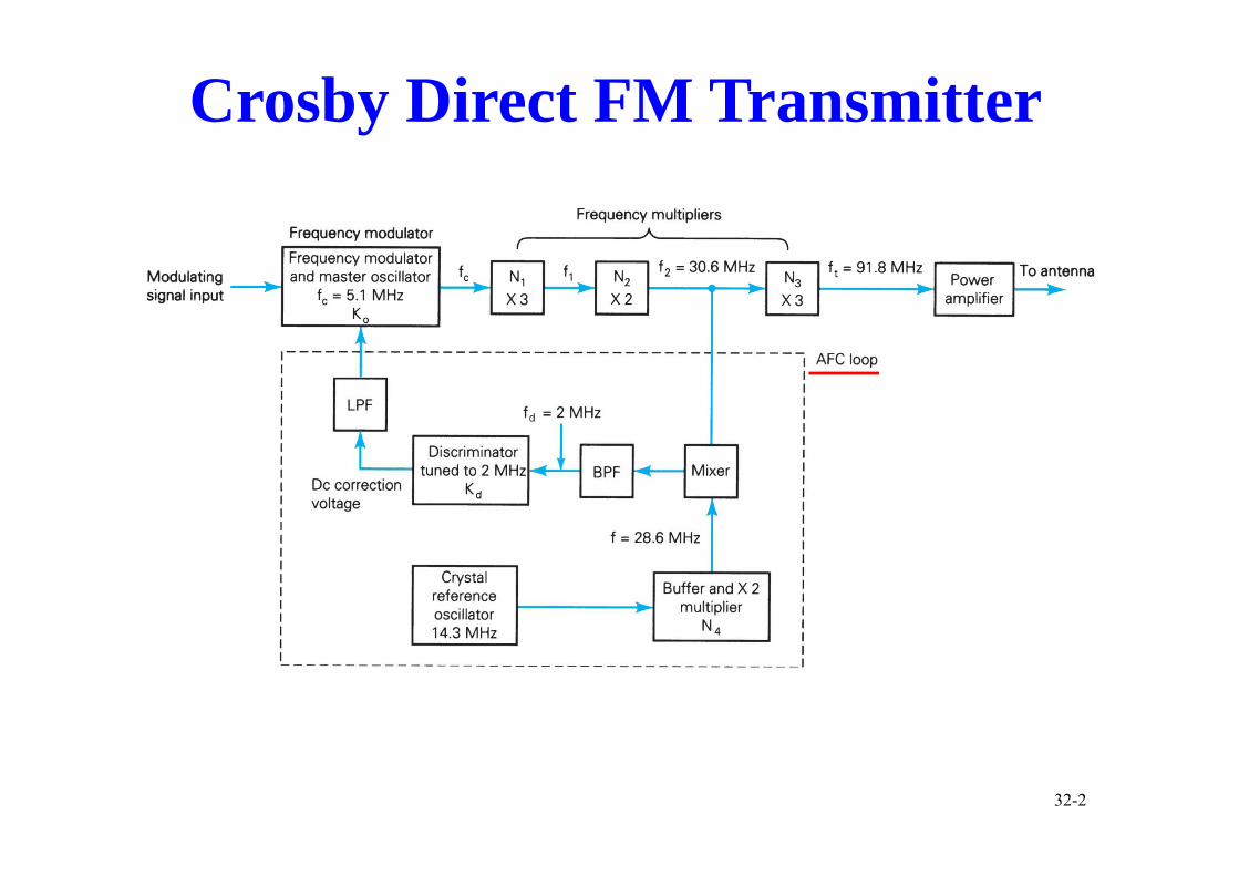
Crosby Direct FM Transmitter
32-2
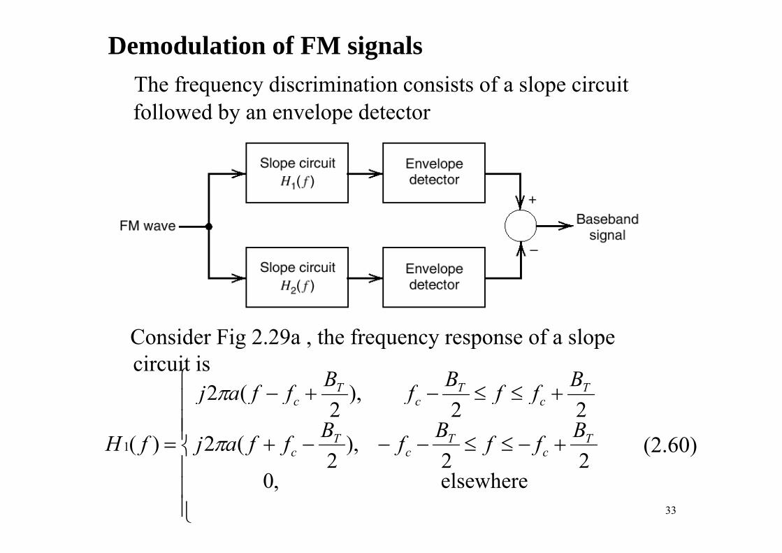
Demodulation of FM signalsThe frequency discrimination consists of a slope circuitThe frequency discrimination consists of a slope circuit followed by an envelope detector
Consider Fig 2 29a the frequency response of a slopeConsider Fig 2.29a , the frequency response of a slope circuit is
22 ),
2(2⎪
⎧ +≤≤−+− Tc
Tc
Tc
BffBfBffaj π
22
),2
(222
),2
(
)(1
⎪
⎪⎪⎪
⎨ +−≤≤−−−+= Tc
Tc
Tc
ccc
BffBf Bffaj
fffffj
fH π (2.60)elsewhere ,0
222
⎪⎪⎪
⎩ 33
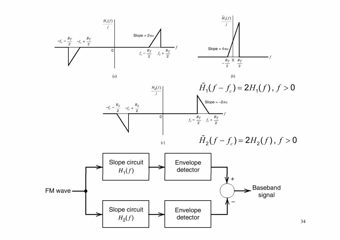
1 1( ) 2 ( ) , 0cH f f H f f− = >%
2 2( ) 2 ( ) , 0cH f f H f f− = >%
34
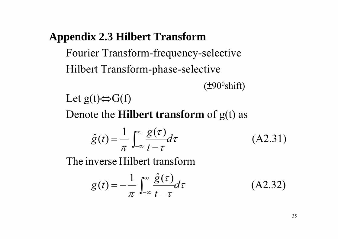
Appendix 2 3 Hilbert TransformAppendix 2.3 Hilbert TransformFourier Transform-frequency-selectiveHilb T f h l iHilbert Transform-phase-selective
(±900shift)Let g(t)⇔G(f)Denote the Hilbert transform of g(t) as g( )
(A2.31) )(1)(ˆ
ττ
τπ
dtgtg ∫
∞
∞−=
)(ˆ1ansformHilbert tr inverse Theτπ t∫ ∞ −
(A2.32) )(ˆ1)(
τ
ττ
πd
tgtg ∫
∞
∞− −−=
35
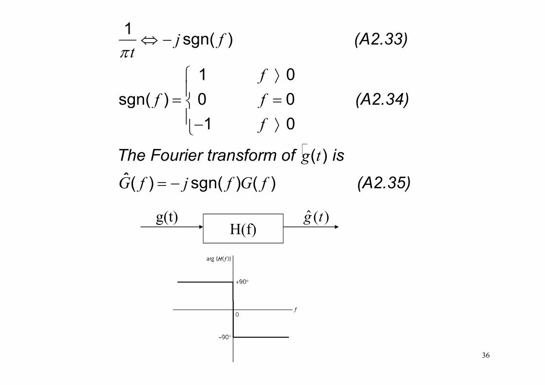
(A2.33)1 sgn( )j ftπ
⇔ −
(A2.34)
1 0sgn( ) 0 0
ff f
⟩⎧⎪= =⎨ ( )
f f
g ( )1 0
( )
f ff
⎨⎪− ⟩⎩
The Fourier transform of is
(A2.35)
( )ˆ( ) sgn( ) ( )
g t
G f j f G f= −
H(f)g(t) )(ˆ tg
( )
36

Properties of the Hilbert Transform( i d i i )(time domain operation)
If g(t) is real
ˆ)(is)(ˆoftransform2.Hilbert
spectrummagnitudesamethehave)(and )(ˆ.1tgtg
tgtg− (take H.F of and ( )g t
)(ˆ)g( 0)(g)g(3.
)(is )(oftransform2.Hilbert
tgtdttt
tgtg
⊥⇒=∫∞
compare with A2.32)( )g t
)()g()(g)g(-
g∫ ∞
37
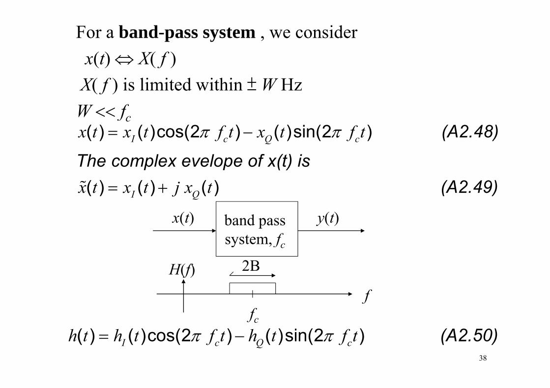
For a band-pass system , we consider x(t) ⇔ X( f )x(t) ⇔ X( f )
X( f ) is limited within ± W HzW fW << fc
(A2.48)( ) ( )cos(2 ) ( )sin(2 )I c Q cx t x t f t x t f tπ π= −
The complex evelope of x(t) is (A2.49)( ) ( ) ( )I Qx t x t j x t= +% ( )( ) ( ) ( )I Qj
band pass system f
x(t) y(t)system, fc
H(f) 2B
fc
f
(A2.50)( ) ( )cos(2 ) ( )sin(2 )I c Q ch t h t f t h t f tπ π= −38
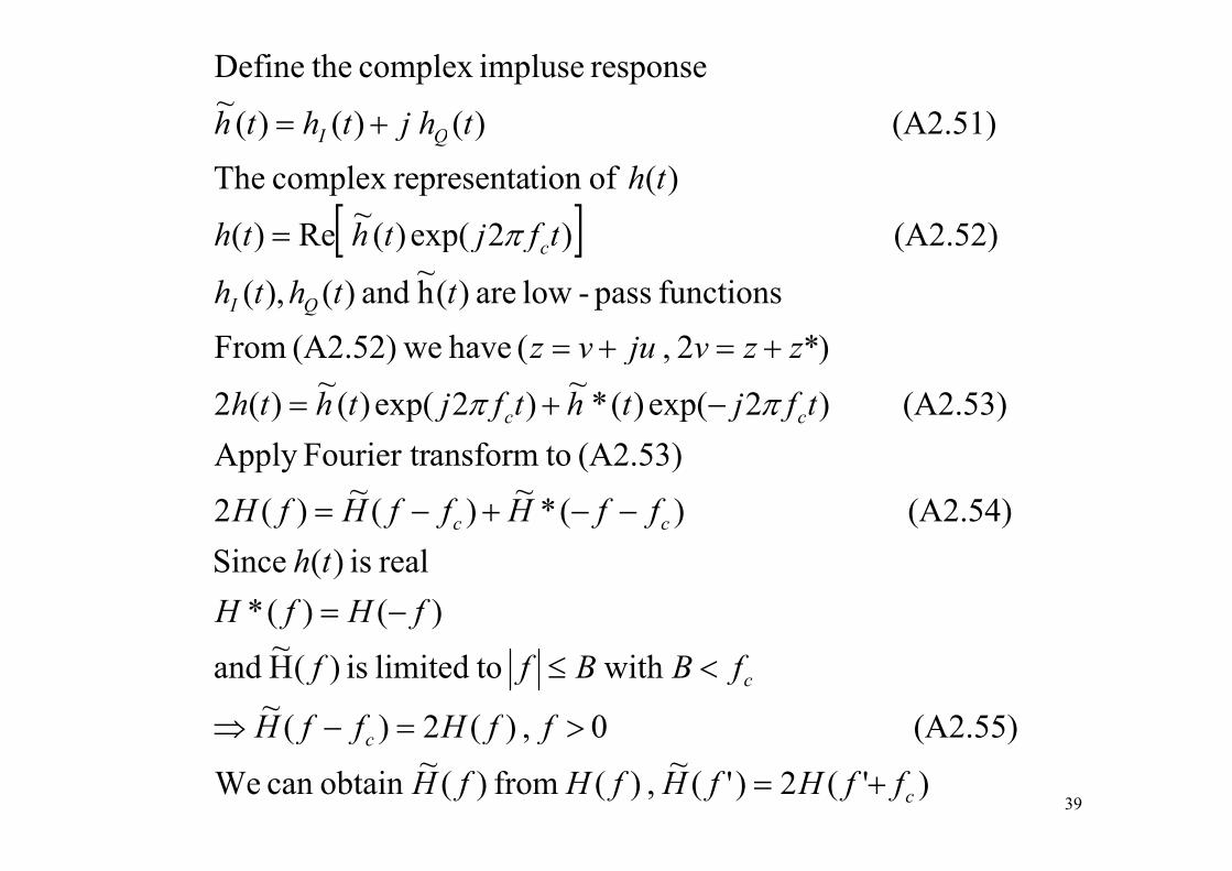
(A2.51) )()()(~ response implusecomplex theDefine
QI tj hthth +=
[ ] (A2 52))2exp()(~Re)(
)( oftion representacomplex The
( ))()()( QI
tfjthth
th
j
= π[ ]
)*2(h(A2 52)F
functions pass-low are )(h~ and )(,)(
(A2.52) )2exp()( Re)(
QI
c
j
tthth
tfjthth = π
(A2.53) )2exp()(*~)2exp()(~)(2
)*2,(havewe(A2.52) From
cc t fjtht fjthth
zzvjuvz
−+=
+=+=
ππ
(A2.54) )(*~)(~)(2
(A2.53) toansformFourier trApply
cc ffHffHfH −−+−=
)()(*real is )( Since
fHfHth
−=
(A2 55)0)(2)(~ with tolimited is )(H~ and c
ffHffH
fBBff
>=−⇒
<≤
)'(2)'(~ , )( from )(~obtain can We
(A2.55) 0,)(2)(
c
c
ffHfHfHfH
ffHffH
+=
>=⇒
39
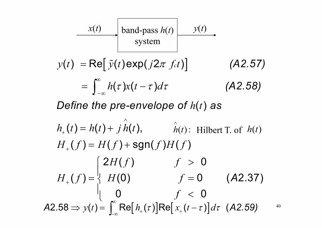
band-pass h(t)x(t) y(t)system
[ ] (A2 57)( ) Re ( )exp( 2 )t t j f t%[ ] (A2.57)
(A2 58)
( ) Re ( )exp( 2 )
( ) ( )
cy t y t j f t
h x t d
π
τ τ τ∞
=
= −∫ (A2.58)
Define the pre-envelope of as
( ) ( )
( )
h x t d
h t
τ τ τ−∞∫
( ) ( ) ( ),h t h t j h t∧
+ = + :)(th∧
Hilbert T. of )(th
( ) ( ) sgn( ) ( )
2 ( )H f H f f H f
H f f+ = +
> 0⎧⎪
( )( ) (0)
0
f fH f H + = A0 ( 2.37)
0f
f
⎧⎪ =⎨⎪⎩ 0 0f⎪ <⎩
40[ ] [ ]A A2.59)2.58 ( ) Re ( ) Re ( ) (y t h x t dτ τ τ∞
+ +−∞⇒ = −∫
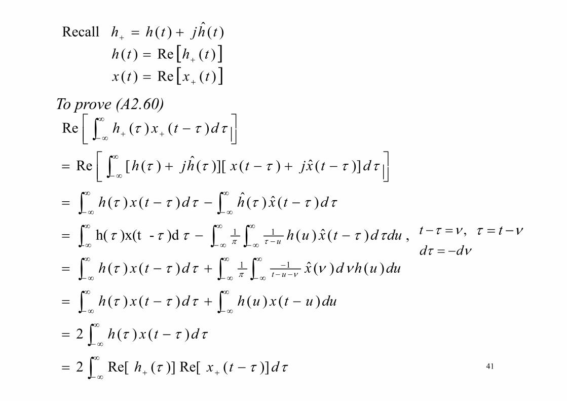
[ ]+
+
=+=
thththjthh)(Re)(
)(ˆ)( Recall
[ ]+= txtx )(Re)(
To prove (A2.60)
∫ +
∞
∞− +
⎤⎡
⎥⎦⎤
⎢⎣⎡ − τττ dtxh )()(Re
p ( )
∫∫
∫∞∞
∞
∞− ⎥⎦⎤
⎢⎣⎡ −+−+=
ττττττ
τττττ
dtxhdtxh
dtxjtxhjh
)(ˆ)(ˆ)()(
)](ˆ)()][(ˆ)([Re
∫∫∫∫∫
∞
∞− −
∞
∞−
∞
∞
∞−∞−
−−=
−−−=
τττττ
ττττττ
τπ dudtxuh
dtxhdtxh
u ,)(ˆ)()d-)x(th(
)()()()(
11-
ντdd
t =− , ντ −= t
∫∫∫∫∫
∫∫∫
∞∞
∞
∞− −−−
∞
∞−
∞
∞−
∞∞∞
+−= νντττ νπ duuhdxdtxh ut )()(ˆ)()( 11ντ dd −=
∫∫∫
∞
∞
∞−
∞
∞−
−=
−+−=
τττ
τττ
dtxh
duutxuhdtxh
)()(2
)()()()(
∫∫
∞
∞− ++
∞−
−= τττ
τττ
dtxh
dtxh
)](Re[)](Re[2
)()(2
41
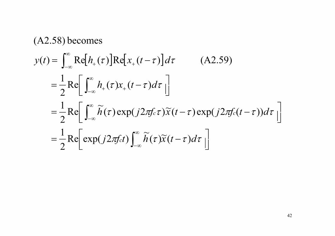
b(A2 58)
[ ] [ ]−= ∫ +
∞
+ (A2.59) )(Re)(Re)(
becomes(A2.58)
τττ dtxhty [ ] [ ]
⎥⎦⎤
⎢⎣⎡ −= ∫
∫
+
∞
∞ +
+∞− +
)()(Re21
( ))()()(
τττ dtxh
y
⎥⎦⎤
⎢⎣⎡ −−=
⎥⎦⎢⎣
∫
∫∞
∞
∞−
))(2exp()(~)2exp()(~Re21
2
ττπττπτ dtfjtxfjh cc
⎥⎦⎤
⎢⎣⎡ −=
⎥⎦⎢⎣
∫
∫∞
∞
∞−
)(~)(~)2exp(Re21
2
τττπ dtxhtfj c ⎥⎦⎢⎣ ∫ ∞−2
42
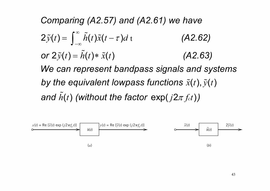
Comparing (A2.57) and (A2.61) we have
(A2.62)
(A2 63)
2 ( ) ( ) ( )
2 ( ) ( ) ( )
y t h t x t dτ τ∞
−∞= −∫ %% %
%
t
or (A2.63)We can represent bandpass signals and systems
2 ( ) ( ) ( )y t h t x t= ∗% %
by the equivalent lowpass functions
and (without the factor )
( ), ( )( ) exp( 2 )
x t y t
h t j f t
% %
%and (without the factor ) ( ) exp( 2 )ch t j f tπ
43
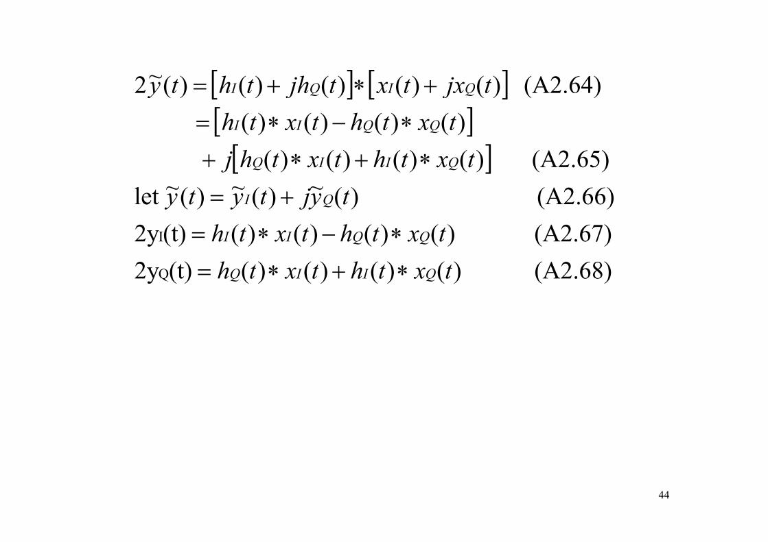
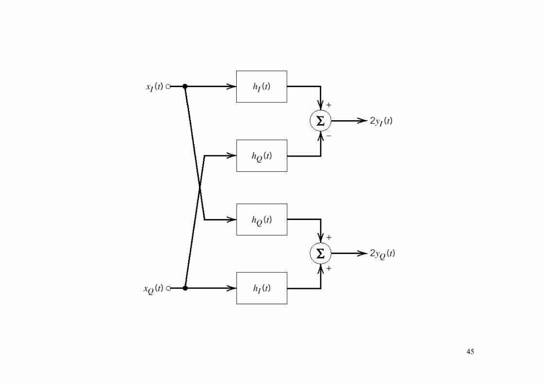
[ ] [ ] (A2 64))()()()()(~2 tjxtxtjhthty QIQI +∗+= [ ] [ ][ ]
[ ])()()()(
(A2.64) )()()()()(2txthtxth
tjxtxtjhthtyQQII
QIQI
∗−∗=+∗+=
[ ](A2.66) )(~)(~)(~let (A2.65) )()()()(
tyjtytytxthtxthj
QI
QIIQ
+=∗+∗+
(A2 68))()()()((t)2y(A2.67) )()()()((t)2y
Q
I
txthtxthtxthtxth
QIIQ
QQII
∗+∗=∗−∗=
(A2.68) )()()()((t)2yQ txthtxth QIIQ ∗+∗=
44
45
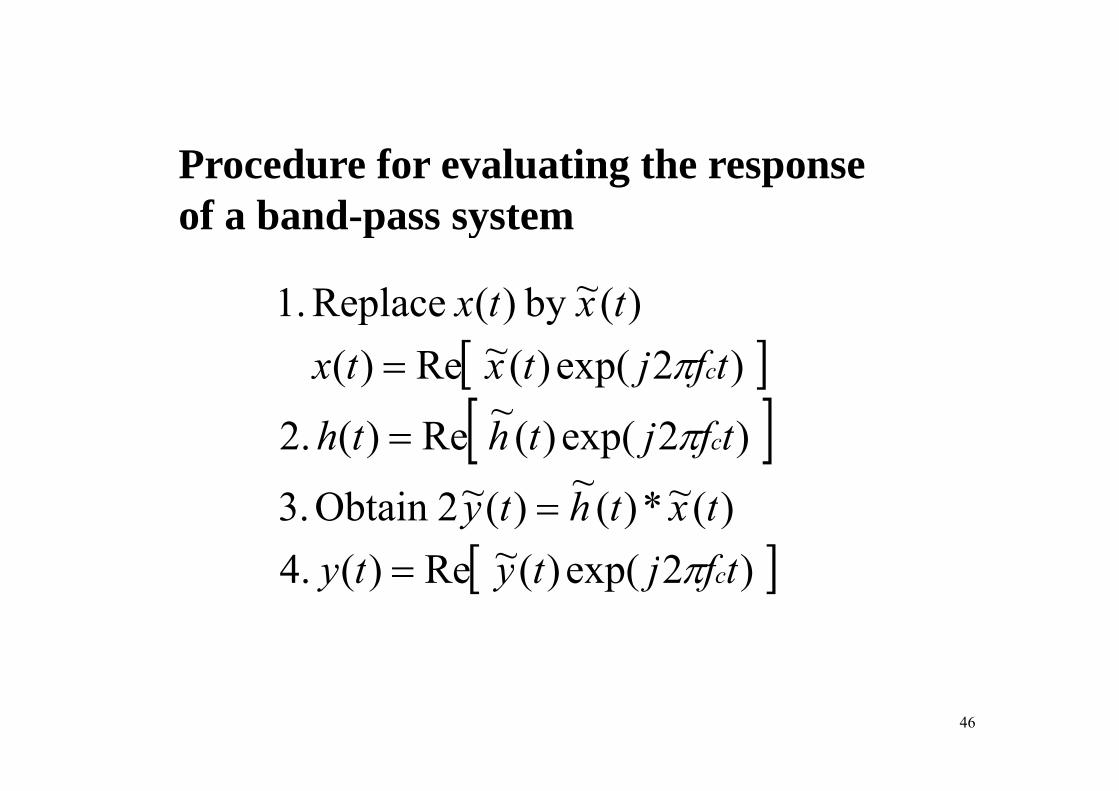
Procedure for evaluating the response of a band pass systemof a band-pass system
)(~by)(Replace1 txtx[ ] )2exp()(~ Re)(
)(by )(Replace 1.tfjtxtx
txtxcπ=
[ ]~
)2exp()(~ Re)( .2 tfjthth cπ=
[ ])2exp()(~Re)(4)(~*)(~)(~2Obtain .3tfjtyty
txthtycπ=
=[ ])2exp()(Re)( .4 tfjtyty cπ=
46
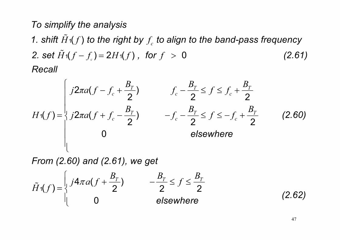
To simplify the analysis 1 shift to the right by to align to the band pass frequency( )H f f%1. shift to the right by to align to the band-pass frequency
2. set , for (2.61)
1
1 1
( )
( ) 2 ( ) 0c
cH f f
H f f H f f− = >%
Recall
2 ( )TBj πa f f− + T TB Bf f f⎧ − ≤ ≤ +⎪
1
2 ( )2
( )
cj πa f f
H f j
+
= (2.60)
2 2
2 ( )2 2 2
c c
T T Tc c c
f f f
B B Bπa f f f f f
≤ ≤ +⎪⎪⎪ + − − − ≤ ≤ − +⎨⎪
elsewhere2 2 2
0
c c c⎨⎪⎪⎪⎩
From (2.60) and (2.61), we getB B B
⎩
⎧
(2.62)elsewhere1
4 ( )( ) 2 2 2
0
T T TB B Bj a f fH f
π⎧ + − ≤ ≤⎪= ⎨⎪⎩
%
elsewhere0⎪⎩
47
t
s t
s t A f t k m dπ π τ τ⎡ ⎤= +⎢ ⎥∫
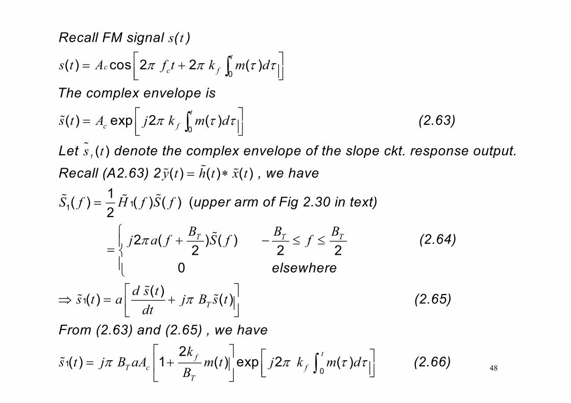
Recall FM signal ( )
( ) cos 2 2 ( )c c fs t A f t k m dπ π τ τ⎡ ⎤= +⎢ ⎥⎣ ⎦
⎡ ⎤
∫The complex envelope is
0( ) cos 2 2 ( )
t
c fs t A j k m d
s t
π τ τ⎡ ⎤= ⎢ ⎥⎣ ⎦∫%
%1
(2.63)
Let denote the complex envelop
0( ) exp 2 ( )
( ) e of the slope ckt. response output.1 p p( )y t h t x t
S f H f S f
= ∗
=
%% %
% %%
p p pRecall (A2.63) 2 , we have
upper arm of Fig 2 30 in text)1
( ) ( ) ( )1( ) ( ) ( ) (
T T T
S f H f S f
B B Bj a f S f fπ
=
⎧ + − ≤ ≤⎪⎨
%
upper arm of Fig 2.30 in text)11( ) ( ) ( ) (2
2 ( ) ( )2 2 2
(2.64)= ⎨
⎪⎩
elsewhere
2 2 20
d s t⎡ ⎤%
( )T
d s ts t a j B s tdt
π⎡ ⎤⇒ = +⎢ ⎥⎣ ⎦% % (2.65)
From (2.63) and (2.65) , we have
1( )( ) ( )
48
tfT c f
T
ks t j B aA m t j k m d
Bπ π τ τ
⎡ ⎤ ⎡ ⎤= +⎢ ⎥ ⎢ ⎥⎣ ⎦⎣ ⎦∫%
(2.66)1
0
2( ) 1 ( ) exp 2 ( )
[ ]
(2.67))(22cos)(2
1
)2exp()(~Re)(
11
⎥⎤
⎢⎡ ++⎥
⎤⎢⎡
+=
=
∫t
ff
T
c
dmktftmk
aAB
t fjtsts
πττπππ
π
(2.67) 2
)(22cos)(10 ⎥⎦⎢⎣
++⎥⎦
⎢⎣
+ ∫fcT
cT dm ktftmB
aAB ττπππ
0sin 2 2 ( )
tc ff t k m dπ π τ τ⎡ ⎤− +⎢ ⎥⎣ ⎦∫⎣ ⎦
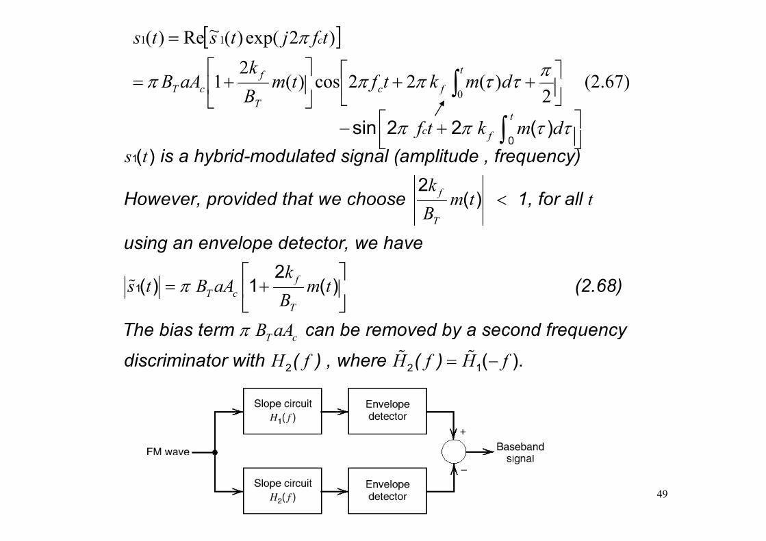
is a hybrid-modulated signal (amplitude , frequency)
However, provided that we choose 1, for all
1( )2
( )f
s tk
m t tB
<
using an envelope detector, we have2
TB
k⎡ ⎤ 1
2( ) 1 ( )f
T cT
ks t B aA m t
Bπ
⎡ ⎤= +⎢ ⎥
⎣ ⎦% (2.68)
The bias term can be removed by a second frequencyB aAπThe bias term can be removed by a second frequency
discriminator with ( ) , where ( )2 2 1( ).T cB aA
H f H f H f
π
= −% %
49
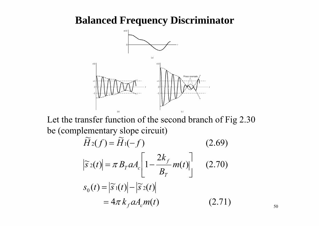
Balanced Frequency Discriminator
~~
Let the transfer function of the second branch of Fig 2.30 be (complementary slope circuit)
(2 70))(2
1)(~
(2.69) )()(
2
12
tmk
aABts
fHfH
fπ ⎥⎤
⎢⎡
=
−=
)(~)(~)(
(2.70) )(1)(
210
2
tststs
tmB
aABtsT
cTπ
−=
⎥⎦
⎢⎣
−=
(2.71) )(4 )()()(0
tmaA k cfπ=50
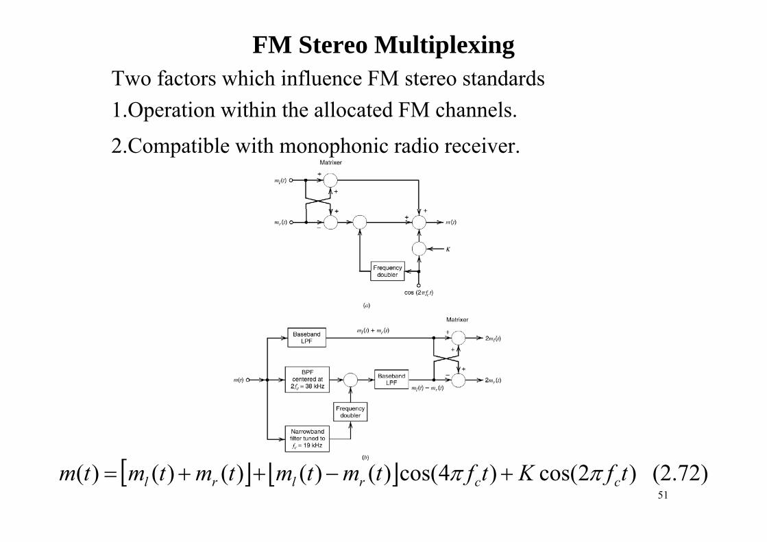
FM Stereo MultiplexingTwo factors which influence FM stereo standards1.Operation within the allocated FM channels.
2 Compatible with monophonic radio receiver2.Compatible with monophonic radio receiver.
[ ] [ ] (2.72) )2cos()4cos()()()()()( t fKt ftmtmtmtmtm ccrlrl ππ +−++=51
Stereo FM
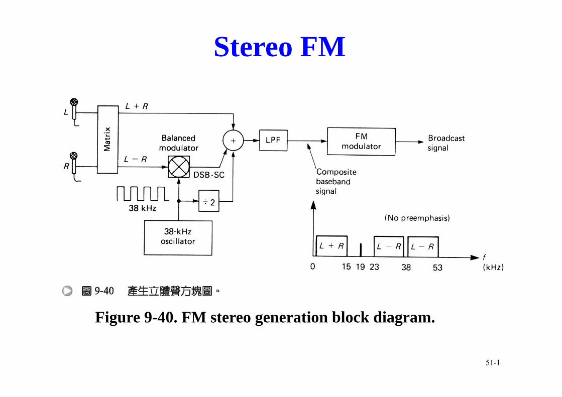
Figure 9-40. FM stereo generation block diagram.
51-1
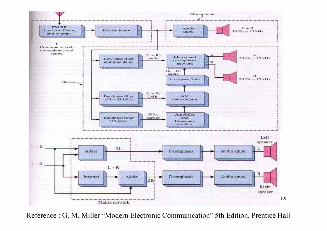
Stereo FM
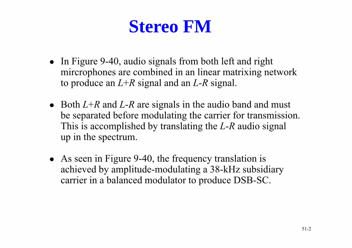
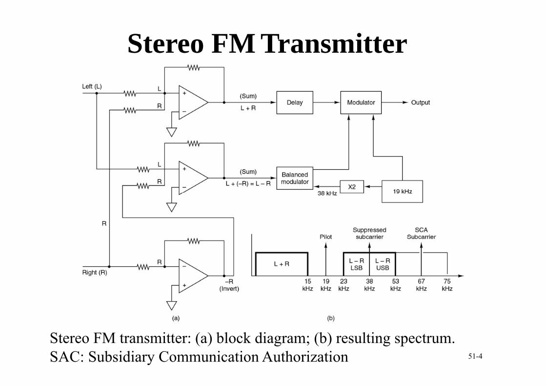
In Figure 9-40, audio signals from both left and right mircrophones are combined in an linear matrixing network to produce an L+R signal and an L-R signal.
Both L+R and L-R are signals in the audio band and must be separated before modulating the carrier for transmission. Thi i li h d b t l ti th L R di i lThis is accomplished by translating the L-R audio signal up in the spectrum.
As seen in Figure 9-40, the frequency translation is achieved by amplitude-modulating a 38-kHz subsidiary carrier in a balanced modulator to produce DSB SCcarrier in a balanced modulator to produce DSB-SC.
51-2
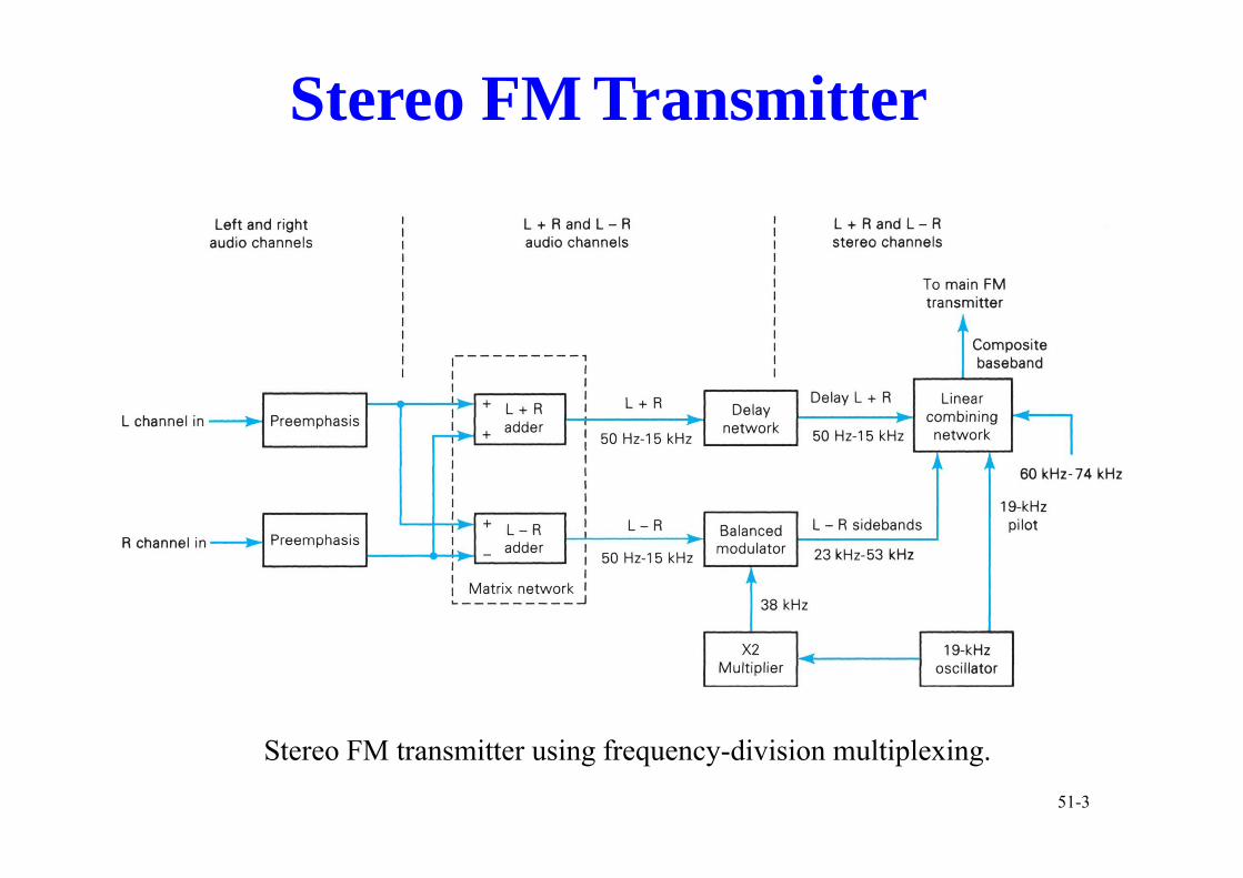
Stereo FM Transmitter
Stereo FM transmitter using frequency-division multiplexing.51-3
Stereo FM Transmitter
Stereo FM transmitter: (a) block diagram; (b) resulting spectrum.SAC: Subsidiary Communication Authorization 51-4
Stereo FM
The stereo receiver will need a frequency-coherent 38-kHz q yreference signal to demodulate the DSB-SC.
To simplify the receiver, a frequency- and phase-coherent signal is derived from the subcarrier oscillator by frequency di i i (÷2) t d il tdivision (÷2) to produce a pilot.
The 19 kHz pilot fits nicely between the L+R and DSB SC LThe 19-kHz pilot fits nicely between the L+R and DSB-SC L-R signals in the baseband frequency spectrum.
51-5
Stereo FMAs indicated by its relative amplitude in the baseband composite signal, the pilot is made small enough so that i FM d i i f h i i l b 10% f hits FM deviation of the carrier is only about 10% of the total 75-kHz maximum deviation.
After the FM stereo signal is received and demodulated to baseband, the 19-kHz pilot is used to phase-lock an p poscillator, which provides the 38-kHz subcarrier for demodulation of the L-R signal.
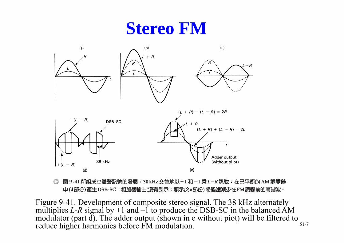
A simple example using equal frequency but unequal amplitude audio toned in the L and R microphones is usedamplitude audio toned in the L and R microphones is used to illustrate the formation of the composite stereo (without pilot) in Figure 9-41.
51-6
Stereo FM
Figure 9-41. Development of composite stereo signal. The 38 kHz alternatelyFigure 9 41. Development of composite stereo signal. The 38 kHz alternately multiplies L-R signal by +1 and –1 to produce the DSB-SC in the balanced AM modulator (part d). The adder output (shown in e without piot) will be filtered to reduce higher harmonics before FM modulation. 51-7
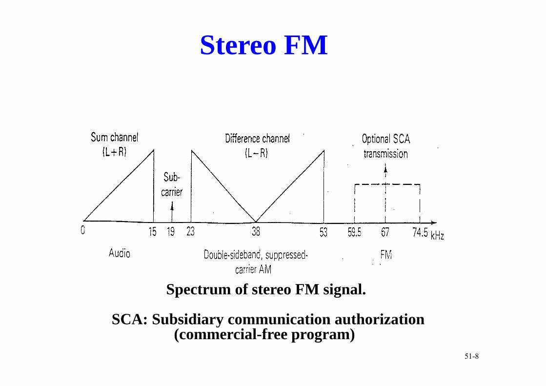
Stereo FM
Spectrum of stereo FM signal.
SCA: Subsidiary communication authorizationy(commercial-free program)
51-8
51-9
Reference : G. M. Miller “Modern Electronic Communication” 5th Edition, Prentice Hall
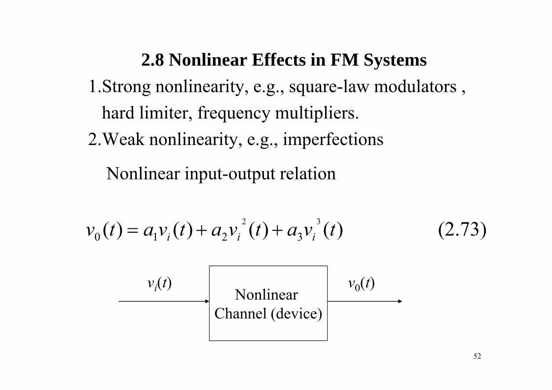
2 8 Nonlinear Effects in FM Systems2.8 Nonlinear Effects in FM Systems1.Strong nonlinearity, e.g., square-law modulators ,
h d li i f l i lihard limiter, frequency multipliers.2.Weak nonlinearity, e.g., imperfections
Nonlinear input-output relation
(2.73) )()()()( 32
3210 tvatvatvatv iii ++= ( ))()()()( 3210 iii
v (t) v (t)Nonlinear
Channel (device)
vi(t) v0(t)
52
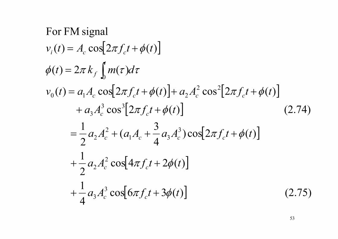
signal FMFor [ ])(2cos)( tt fAtvt
cci φπ +=
∫[ ] [ ])(2cos)(2cos)(
)(2)(22
0
ttfAattfAatv
dm kt f
φπφπ
ττπφ
+++=
= ∫[ ] [ ]
[ ] (2.74) )(2cos
)(2cos)(2cos)(33
3
210
tt fAa
ttfAattfAatv
cc
cccc
φπ
φπφπ
++
+++=
[ ])(2cos)43(
21 3
312
2 tt fAaAaAa cccc φπ +++=
[ ])(24cos21 2
2 tt fAa cc φπ ++
[ ] (2.75) )(36cos41
23
3 tt fAa cc φπ ++4
53
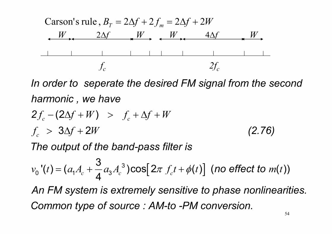
WfffB mT 2222 , rule sCarson' +Δ=+Δ=W W W WfΔ4fΔ2W W W WfΔ4fΔ2
f 2ffc 2fc
In order to seperate the desired FM signal from the second harmonic , we have2 (2 )f f W f f W− Δ + > + Δ +2
(2.76)Th t t f th b d fil
(2 )3 2
c c
c
f f W f f Wf f W
Δ + > + Δ +
> Δ +
t iThe output of the band-pass fil
[ ]
ter is
no effect to33'( ) ( )cos 2 ( ) ( ( ))v t a A a A f t t m tπ φ= + +[ ] no effect to
An FM system is extremely sensitive to phase nonlinearities.
0 1 3( ) ( )cos 2 ( ) ( ( ))4c c cv t a A a A f t t m tπ φ= + +
Common type of source : AM-to -PM conversion.54
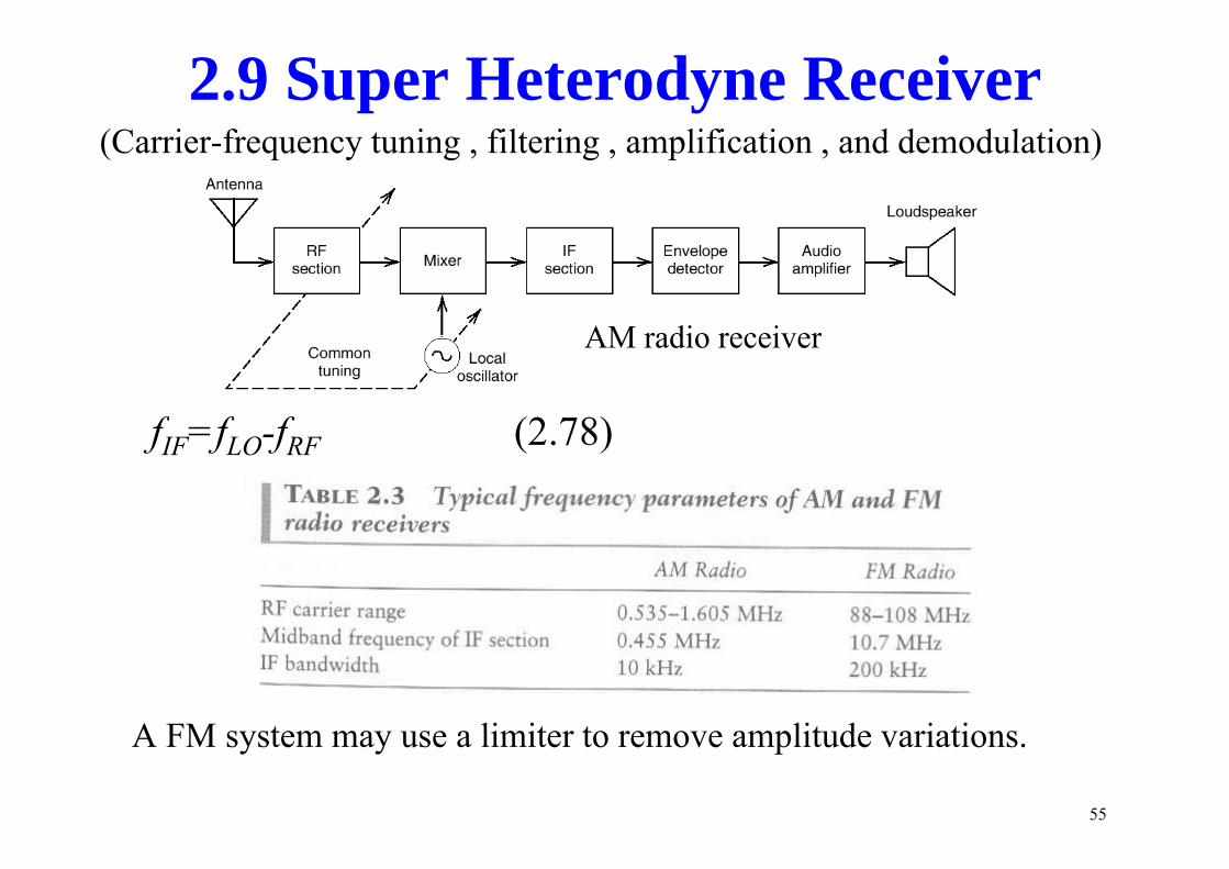
2.9 Super Heterodyne Receiver(Carrier frequency tuning filtering amplification and demodulation)(Carrier-frequency tuning , filtering , amplification , and demodulation)
AM radio receiver
f =f -f (2 78)
AM radio receiver
fIF=fLO-fRF (2.78)
A FM t li it t lit d i tiA FM system may use a limiter to remove amplitude variations.
55
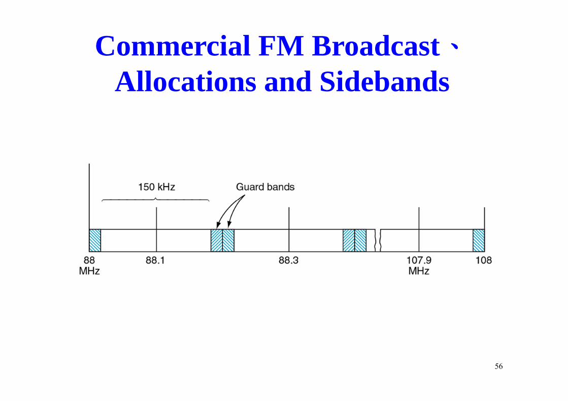
Commercial FM Broadcast、Allocations and Sidebands
56
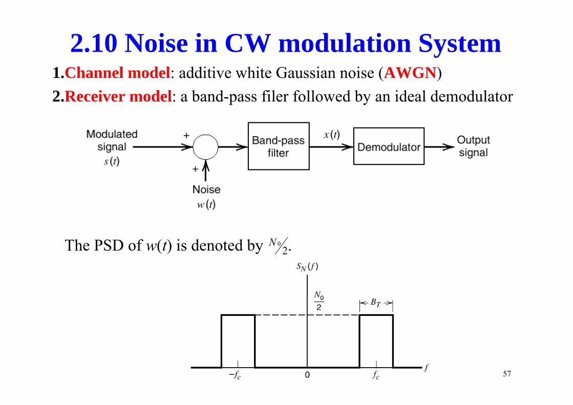
2.10 Noise in CW modulation System1.Channel model: additive white Gaussian noise (AWGN)2.Receiver model: a band-pass filer followed by an ideal demodulator
The PSD of w(t) is denoted by 20NThe PSD of w(t) is denoted by .2
57
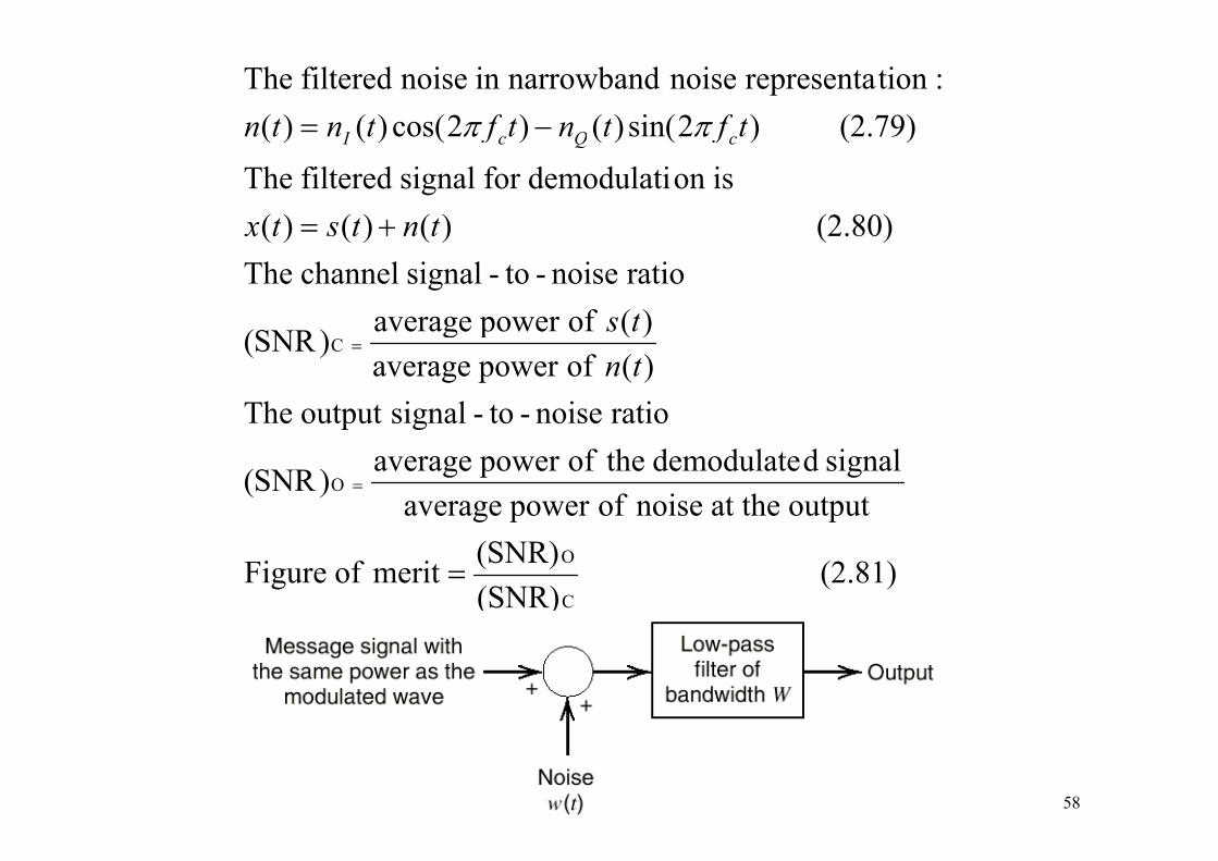
(2.79) )2sin()()2cos()()(:tionrepresenta noise narrowbandin noise filtered The
−= t ftntftntn cQcI ππ
(2.80))()()(ison demodulatifor signal filtered The
( ))()()()()(
+= tntstx
ff cQcI
)(ofpower average)SNR(
ratio noise-to-signal channel The(2.80) )()()( +
ts
tntstx
ratio noise-to-signaloutput The)( ofpower average)(pg)SNR( C =
tn
output at the noise ofpower averagesignal ddemodulate theofpower average)SNR( O =
(2.81) (SNR)(SNR)merit of Figure
C
O=
58
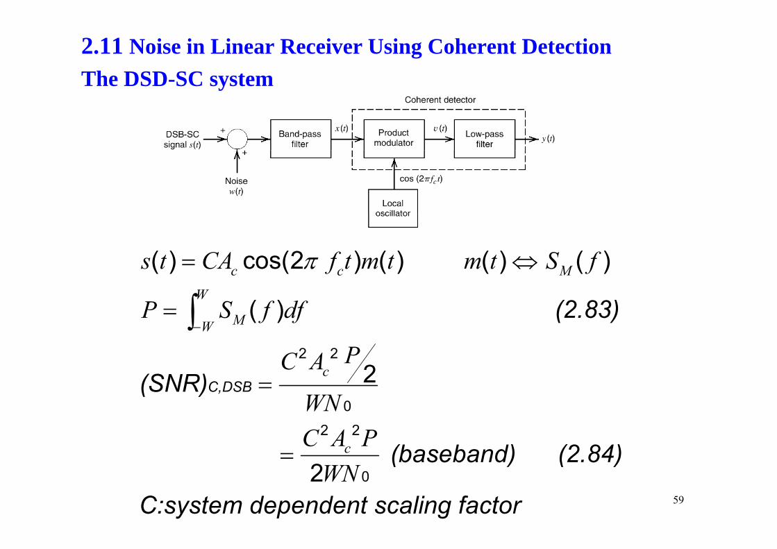
2.11 Noise in Linear Receiver Using Coherent DetectionThe DSD-SC systemy
( ) cos(2 ) ( ) ( ) ( )c c Ms t CA f t m t m t S fπ= ⇔
(2.83)( )
c c M
W
MWP S f df
−= ∫
C,DSB(SNR)2 2
2cPC A
WN=
(baseband) (2.84)
0
2 2c
WNC A P
= (baseband) (2.84)
C:system dependent scaling factor02WN
59
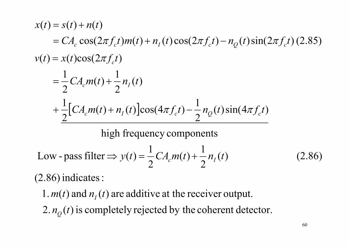
(2 85))2sin()()2cos()()()2cos()()()(
tftntftntmtfCAtntstx
++=
πππ
)2()cos()(
(2.85))2sin()()2cos()()()2cos(
t ftxtv
tftnt ftntmtfCA
c
cQcIcc
=
−+=
π
πππ
)(21)(
21 tntmCA Ic +=
[ ] )4sin()(21)4cos()()(
21 t ftnt ftntmCA cQcIc −++ ππ
11componentsfrequency high
:indicates(2 86)
(2.86) )(21)(
21)(filter pass-Low tntmCAty Ic +=⇒
d t th tb thj t dl t li)(2output.receiver at the additive are )( and )( 1.
:indicates(2.86)
ttntm I
detector.coherent by therejectedcompletely is )( 2. tnQ
60
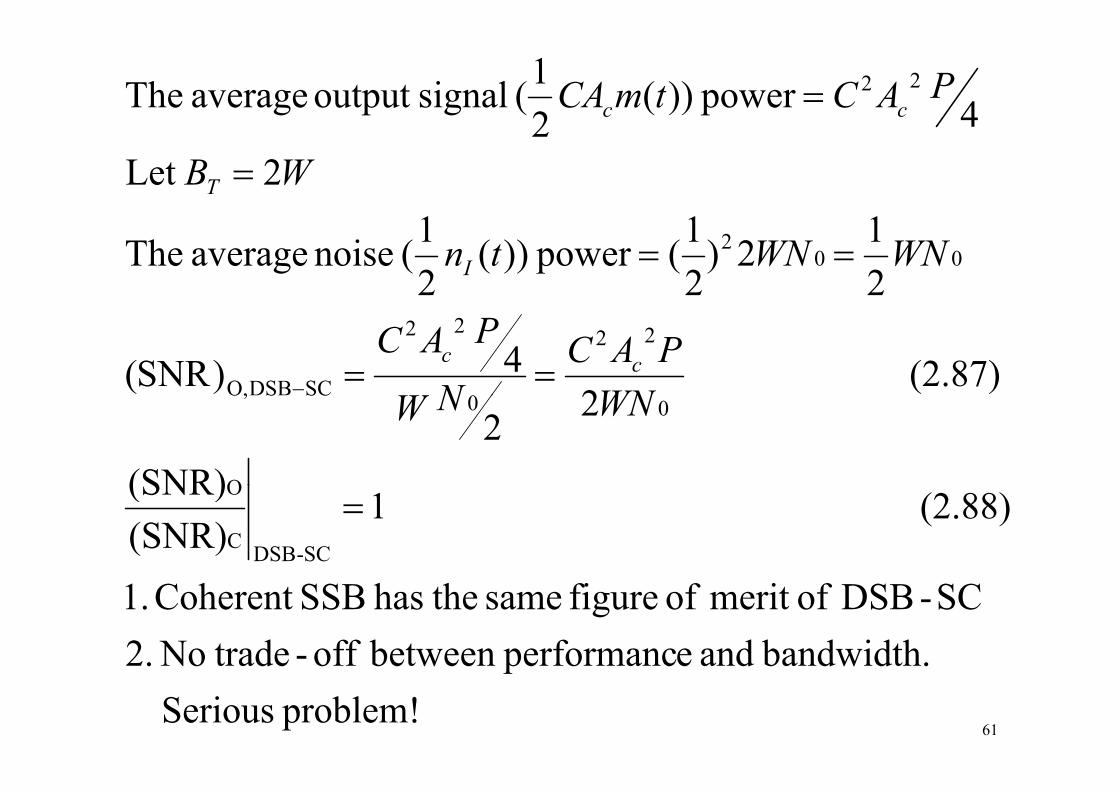
4power ))(21( signaloutput average The 22= PACtmCA cc
2Let 42
= WBT
212)
21(power ))(
21( noise average The 00
2 == WNWNtnI
(2.87) 2
4)SNR(22
0
22
SCDSBO, ==− WNPAC
NW
PACcc
(SNR)
22O
00SCSO, WNNW
(2.88) 1(SNR)(SNR)
SC-DSBC
O=
bandwidth.andeperformancbetweenoff-tradeNo2.SC-DSB ofmerit of figure same thehas SSBCoherent 1.
problem! Serious bandwidth.andeperformancbetween offtradeNo 2.
61
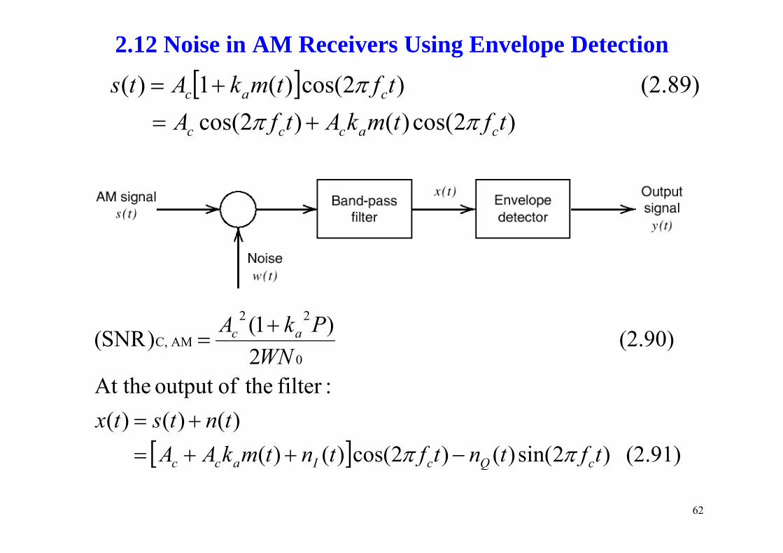
2.12 Noise in AM Receivers Using Envelope Detection
[ ] (2 89))2cos()(1)( tftmkAts π+= [ ])2cos()()2cos(
(2.89) )2cos()(1)(t ftmkAt fA
tftmkAts
caccc
cac
πππ
+=+=
(2 90))1()SNR(22
AMCPkA ac +
=
:filter theofoutput At the
(2.90) 2
)SNR(0
AMC,WN
=
[ ] (2.91) )2sin()()2cos()()( )()()(
tftntftntmkAAtntstx
cQcIacc ππ −++=+=
[ ] ( ))()()()()( ff cQcIacc
62
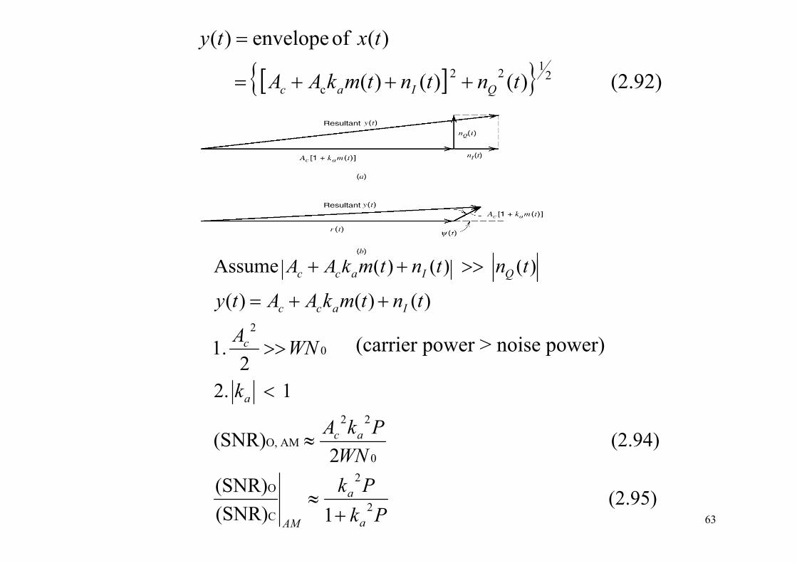
[ ]{ } (2.92) )()()(
)( of envelope)(2
1 22 c tntntmkAA
txty
QIac +++=
=
[ ]{ } ( ))()()(c QIac
)( )()( Assume tntntmkAA QIacc >>++
1
)()()(2
WNA
tntmkAAty
c
Iacc
>>
++=
(carrier power > noise power)
1 2.2
.1 0
k
WN
a
c
<
>> (carrier power > noise power)
(2.94) 2
(SNR)0
22
AMO,WN
PkA ac≈
(2.95) 1(SNR)
(SNR)2
2
C
O
PkPk
a
a
AM +≈
63
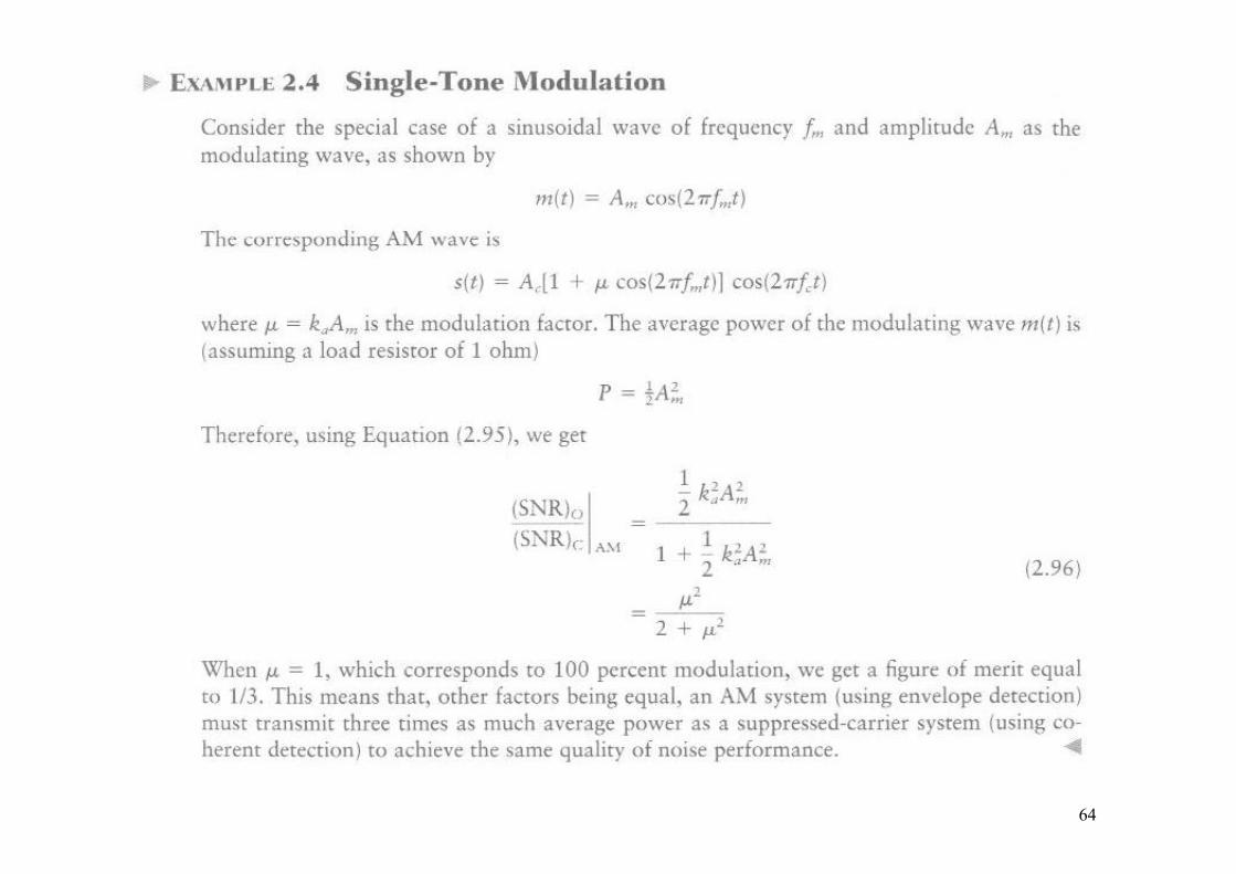
64
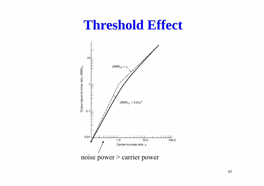
Threshold Effect
noise power > carrier power
65
noise power > carrier power
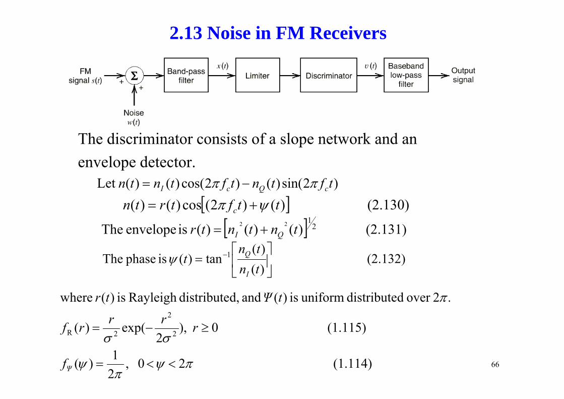
2.13 Noise in FM Receivers
The discriminator consists of a slope network and an envelope detector.
)2sin()()2cos()()(Let t ftnt ftntn cQcI ππ −=
[ ] ( ))()()()( f[ ] (2.130) )()2(cos)()( ttftrtn c ψπ +=
[ ] (2.131) )()()( is envelope The 2122 tntntr QI +=
)( ⎤⎡(2.132)
)()(
tan)( is phase The 1⎥⎦
⎤⎢⎣
⎡= −
tntn
tI
Qψ
(1.115) 0 ),2
exp()(
.2over ddistributeuniformis)(andd,distributeRayleigh is)(where
2
2
2R
π
≥−= rrrrf
tΨtr
(1.114) 2 0 ,21)(
2 22
πψπ
ψ
σσ
<<=Ψf 66
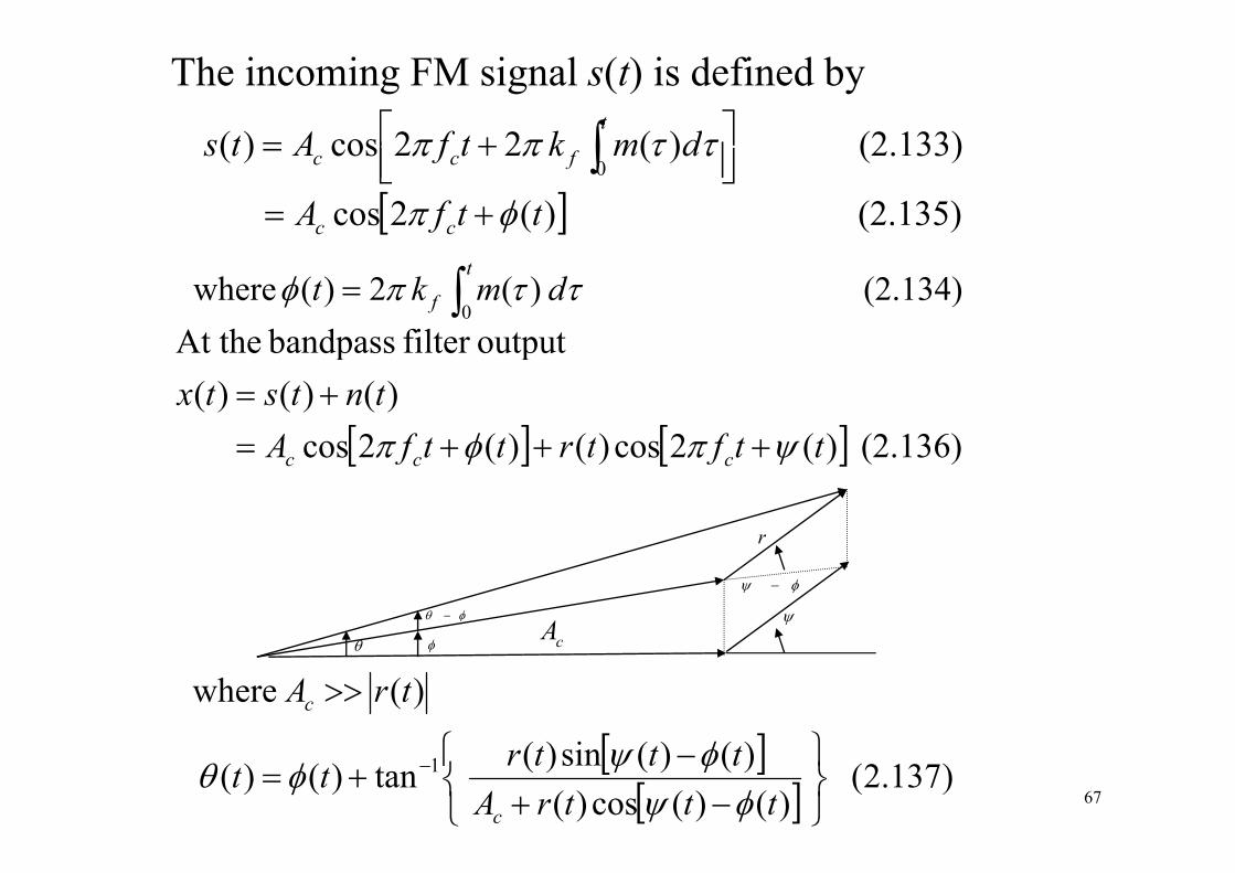
The incoming FM signal s(t) is defined by
(2 133))(22cos)( ⎤⎡ + ∫t
dktfAt (2.133) )(22cos)(0 ⎥⎦
⎤⎢⎣⎡ += ∫fcc dmktfAts ττππ
[ ] (2.135) )(2cos tt fA cc φπ +=
(2.134) )(2)( where
0 ττπφ dm kt
t
f ∫=
outputfilterbandpassAt the
[ ] [ ] (2 136))(2)()(2)()()(
outputfilter bandpass At the
ffAtntstx
φ+=
[ ] [ ] (2.136) )(2cos)()(2cos tt ftrttfA ccc ψπφπ +++=
r
φψ −
ψ
r
φθ −
A
[ ])( where
⎫⎧
>> trAc
θ φ cA
[ ][ ] )137.2(
)()(cos)()()(sin)( tan)()( 1
⎭⎬⎫
⎩⎨⎧
−+−
+= −
tttrAtttrtt
c φψφψφθ
67
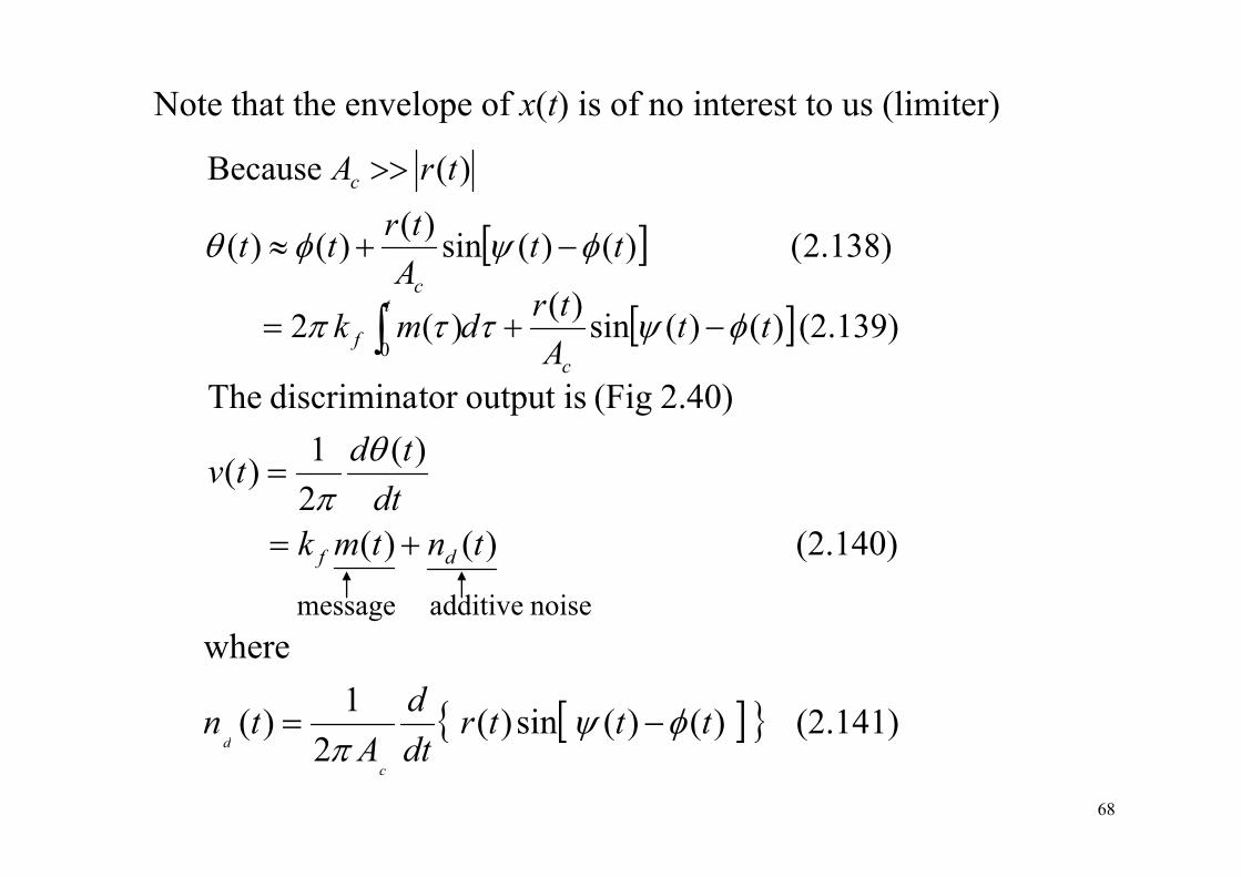
Note that the envelope of x(t) is of no interest to us (limiter)
[ ] )1382()()(i)()()(
)( Because
tttrtt
trAc
φφθ +
>>
[ ] )138.2( )()(sin)()()( ttA
ttc
φψφθ −+≈
[ ](2.139))()(sin)()(2 tttrdm kt
f φψττπ −+= ∫ [ ]( ))()()(0 Ac
f φψ∫
)(12.40) (Fig isoutput tor discrimina The
dθ
(2 140))()(
)(21)(
ttkdt
tdtv
+
=θ
π
hnoise additivemessage
(2.140) )()( tntmk df +=
[ ]{ } (2.141) )()(sin)(2
1)(
where
tttrdd
Atn
dφψ −= [ ]{ } ( ))()()(
2)(
dt Ac
dφψ
π68
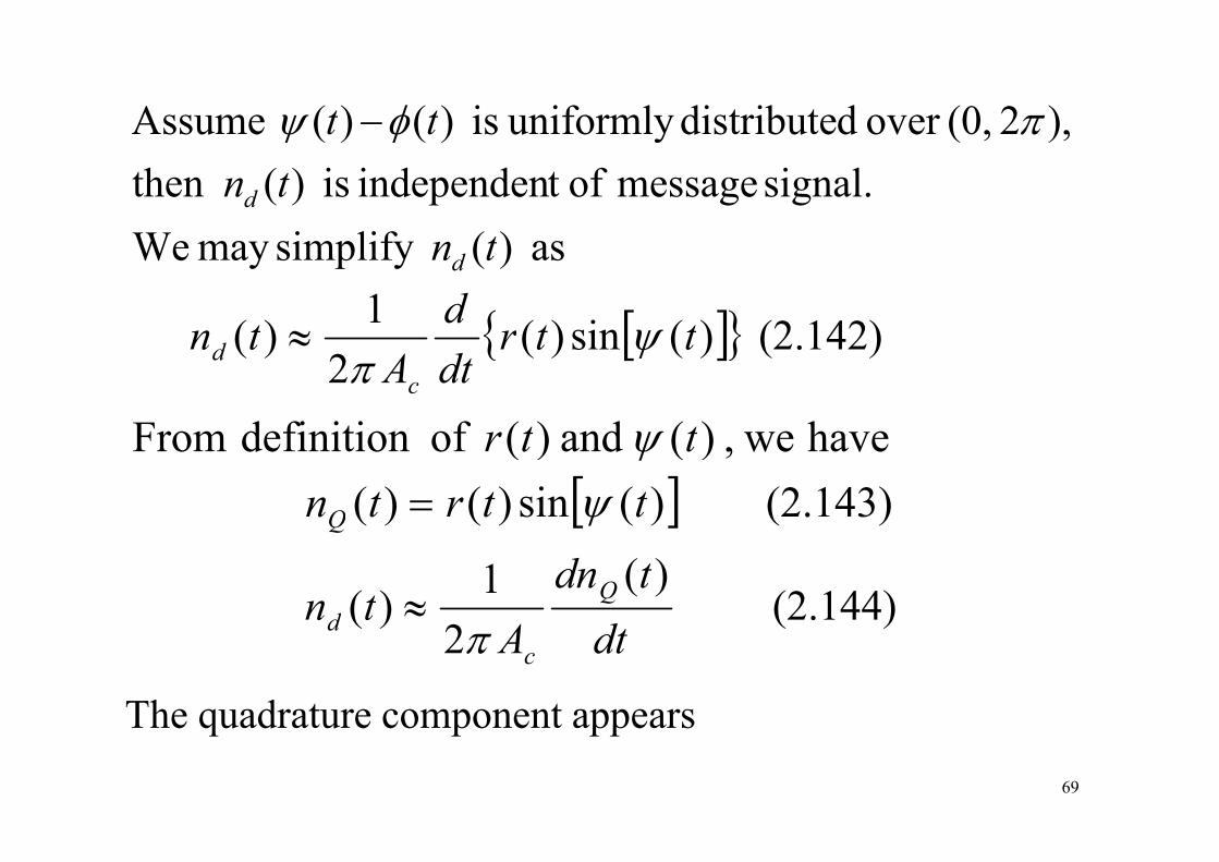
),2(0,over ddistributeuniformly is )()( Assume tt πφψ −
)(i lifWsignal. message oft independen is )(then
),( ,y)()(tnd
φψ
[ ]{ } (2 142))(sin)(1)( ttrdtn ψ≈
as )(simplify may We tnd
[ ]{ } (2.142) )(sin)(2
)( ttrdt A
tnc
d ψπ
≈
h)(d)(fd fi itiF tt[ ] (2.143) )(sin)()(
havewe,)(and)(ofdefinitionFromttrtn
ttr
Q ψψ
=Q
(2.144) )(
21)(
dtdn
Atn Q
d ≈ ( )2
)(dtAc
d π
The quadrature component appearsThe quadrature component appears69
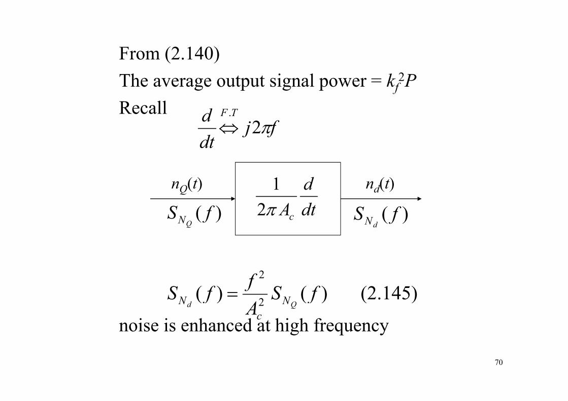
From (2.140)The average output signal power = kf
2PRecall d TFRecall
fjdtd TF
π2.
⇔
nQ(t) nd(t)d1dtAcπ2)( fS
QN )( fSdN
(2 145))()(2
fSffSnoise is enhanced at high frequency
(2.145) )()( 2 fSA
fSQd N
cN =
70
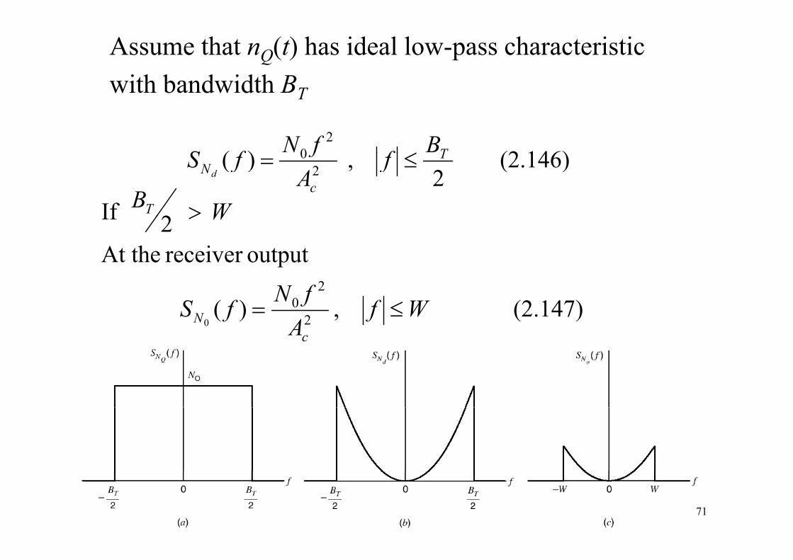
Assume that nQ(t) has ideal low-pass characteristic with bandwidth BTwith bandwidth BT
(2 146))(2
0 TBffNfS ≤ (2.146) 2
, )( 20 T
cN f
AffS
d≤=
2 If WBT >
output receiver At the
2If W>
(2.147) , )( 2
20
0Wf
AfNfSc
N ≤=
71
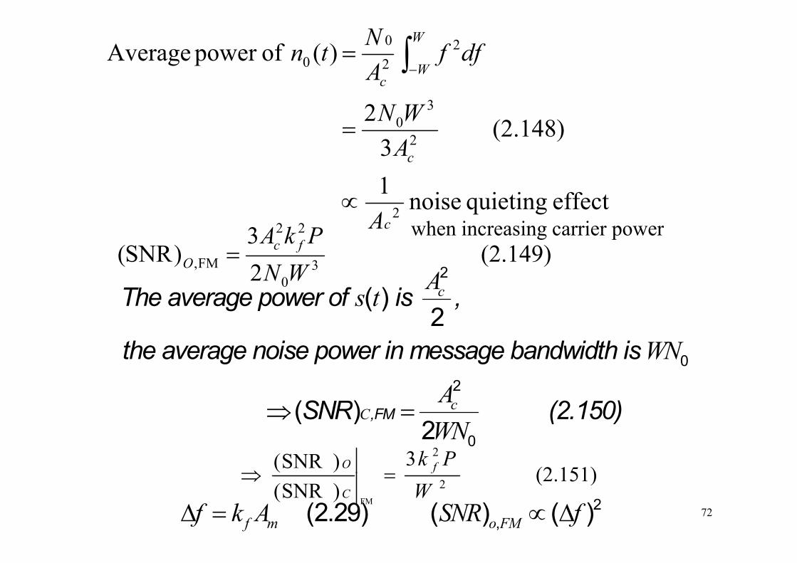
)( ofpower Average
22
00
W
Wc
dffANtn = ∫−
(2.148) 3
2 2
30
AWN
=
effect quieting noise 1
3
2
c
A
A
∝cA
(2.149) 23
)SNR( 30
22
FM, WNPkA fc
O =2A
when increasing carrier power
0The average power of is ,
the a erage noise po er in message band idth is
( )2cAs t
WN
FM
the average noise power in message bandwidth is
SNR (2 150)
02
( ) cC
WN
A⇒ ,FM SNR (2.150)
0
( )2
cC
WN⇒ =
(2 151)3)SNR( 2 Pk fO
⇒2
,(2.29) ( ) ( )f m o FMf k A SNR fΔ = ∝ Δ
(2.151) )SNR( 2
FMW
f
C=⇒
72
⎥⎤
⎢⎡ Δ
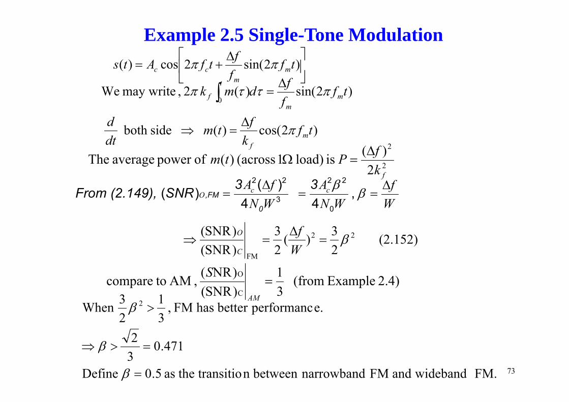
+= )2sin(2cos)( tfftfAts ππ
Example 2.5 Single-Tone Modulation⎥⎦
⎢⎣
+= )2sin(2cos)( tff
tfAts mm
cc ππ
)2sin()(2 , may write We0
t fffdm k mm
t
f πττπ Δ=∫
)2cos()( sideboth t fk
ftmdtd
mf
πΔ=⇒
2)(il d)1()(fTh fP ΔΩ 22
)(is load)1(across)(ofpower averageThefk
fPtm =Ω
,FM3 3From (2.149), SNR
2 2 2 2
3
( )( ) ,4 4
c cO
A f A fN W N W W
ββ
Δ Δ= = =
03
04 4N W N W W
(2.152) 23)(
23
)SNR()SNR( 22 β=
Δ=⇒
WfO
2.4) Example (from 31
)SNR()NR( , AM tocompare
C
O=
S
22)SNR( FM WC
3)SNR( C AM
2
e.performancbetter has FM , 31
23When 2 >β
FM. widebandand FM narrowbandbetween n transitio theas 5.0 Define
471.032
=
=>⇒
β
β
73
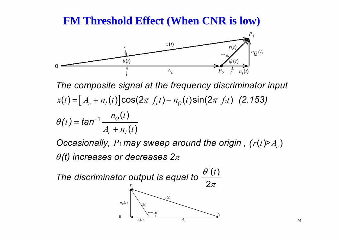
FM Threshold Effect (When CNR is low)
When there is no signal, i.e., carrier is unmodulated. The composite signal at the frequency discriminator input
[ ] (2.153)
( ) t 1
( ) ( ) cos(2 ) ( )sin(2 )
( )
cc I c Q
Q
x t A n t f t n t f t
n t
π π
θ −
= + −
( ) tan
Occasionally,
1 ( )( )
Q
c I
tA n t
θ =+
may sweep around the origin , ( >1 ( ) )cP r t Ay,
'
y p g , ((t) increases or decreases 2
Th di i i t t t i l t
( ) )
( )
c
tθ π
θThe discriminator output is equal to ( )2
tθπ
( )r(t)
P1
nQ(t) x(t)
Ac0 P2
θnI(t) 74
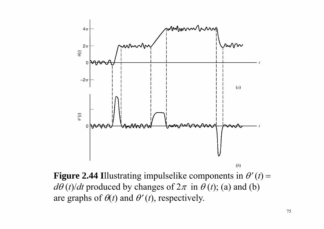
Figure 2.44 Illustrating impulselike components in θ′ (t) =dθ (t)/dt produced by changes of 2π in θ (t); (a) and (b) are graphs of θ(t) and θ′ (t), respectively.
75
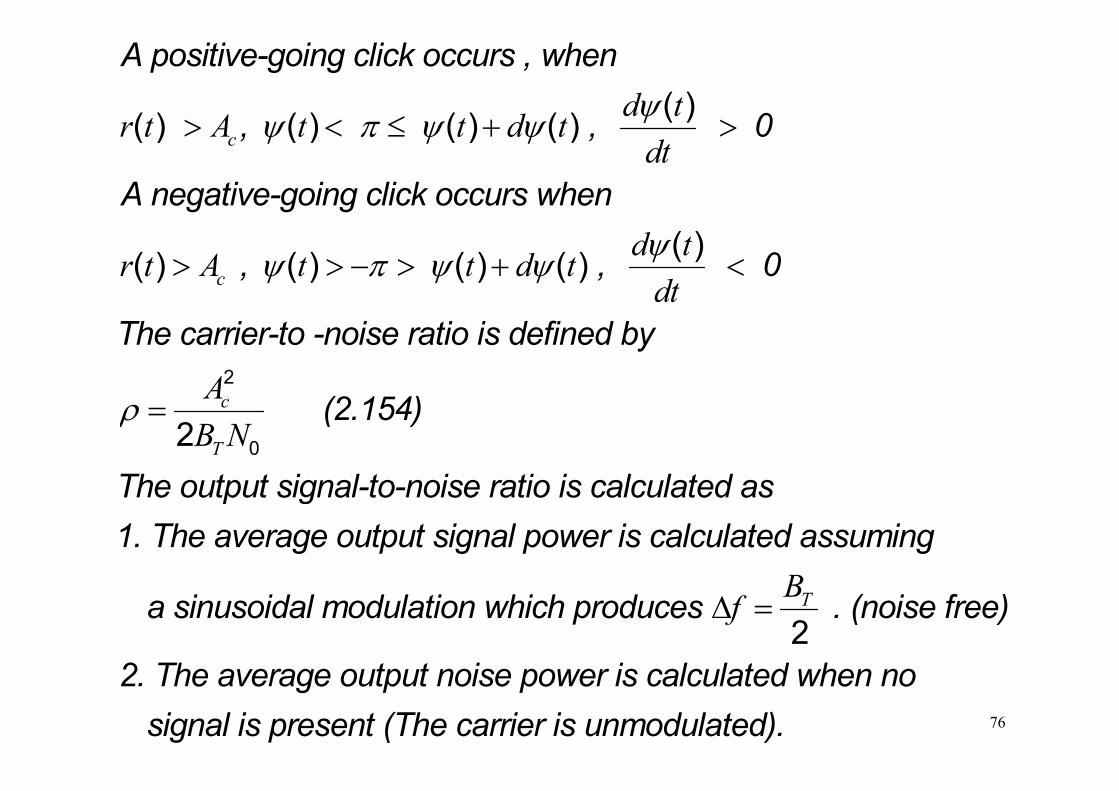
d tr t A t t d t ψψ π ψ ψ> < ≤ + >
A positive-going click occurs , when
0( )( ) ( ) ( ) ( )cr t A t t d tdt
ψ π ψ ψ> < ≤ + > , , 0
A negative-going click occurs when
( ) ( ) ( ) ( )
cd tr t A t t d t
dtψψ π ψ ψ> > − > + < , , 0( )( ) ( ) ( ) ( )
The carrier-to -noise ratio is definA
ed by 2c
T
AB N
ρ = (2.154)
The output signal to noise ratio is calculated as02
B
The output signal-to-noise ratio is calculated as1. The average output signal power is calculated assuming
TBfΔ = a sinusoidal modulation which produces . (noise free)
22
Th t t i i l l t d h2. The average output noise power is calculated when no signal is present (The carrier is unmodulated). 76
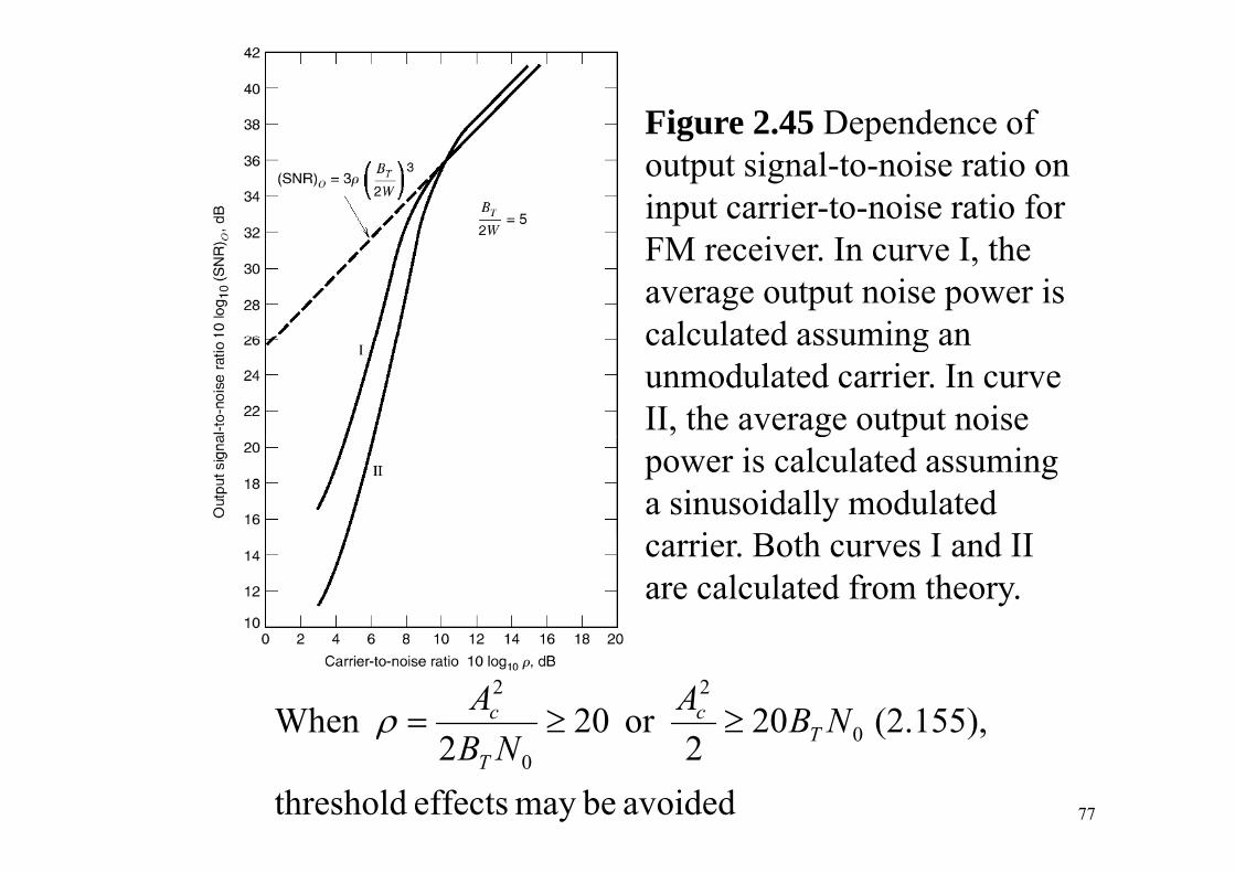
Figure 2.45 Dependence of g poutput signal-to-noise ratio on input carrier-to-noise ratio for FM i I I hFM receiver. In curve I, the average output noise power is calculated assuming ancalculated assuming an unmodulated carrier. In curve II, the average output noise g ppower is calculated assuming a sinusoidally modulated
i B th I d IIcarrier. Both curves I and II are calculated from theory.
(2.155),20or 20When 0
22
NBAAT
cc ≥≥=ρ
avoided bemay effects threshold
( ),22 0
0NB TT
ρ
77
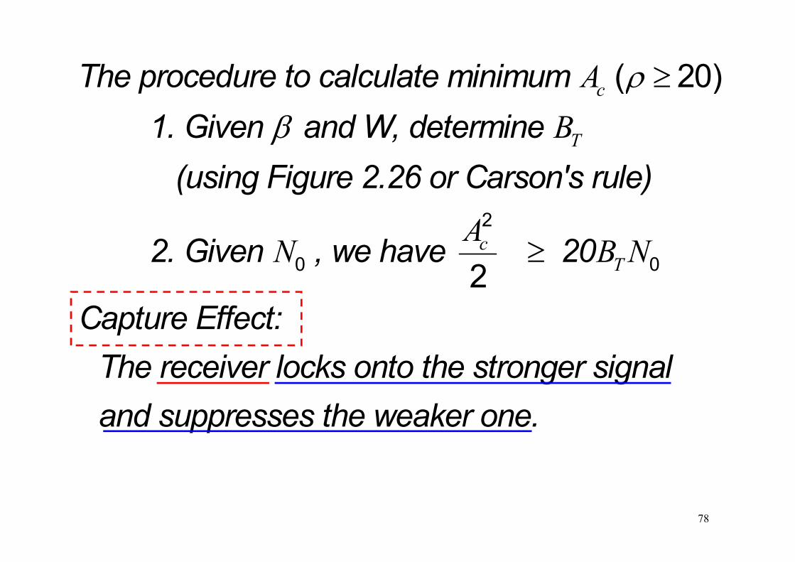
The procedure to calculate minimum ( 20)cA ρ ≥p 1. Given and W, determine
( )c
TBρ
β (using Figure 2.26 or Carson's rule)
2
2. Given , we have 202
0 02c
TAN B N≥
Capture Effect:2
The receiver locks onto the stronger signald th k and suppresses the weaker one.
78
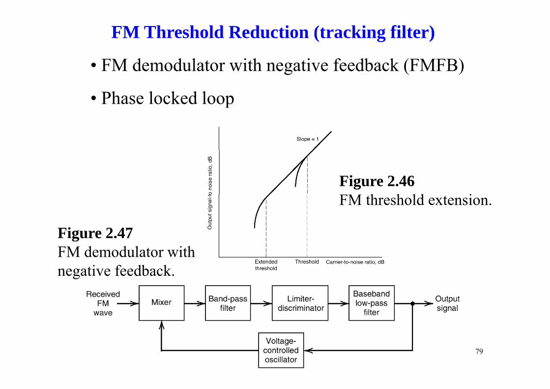
FM Threshold Reduction (tracking filter)
FM d d l t ith ti f db k (FMFB)• FM demodulator with negative feedback (FMFB)
• Phase locked loopp
Figure 2.46 FM h h ld iFM threshold extension.
Figure 2.47 gFM demodulator with negative feedback.
79
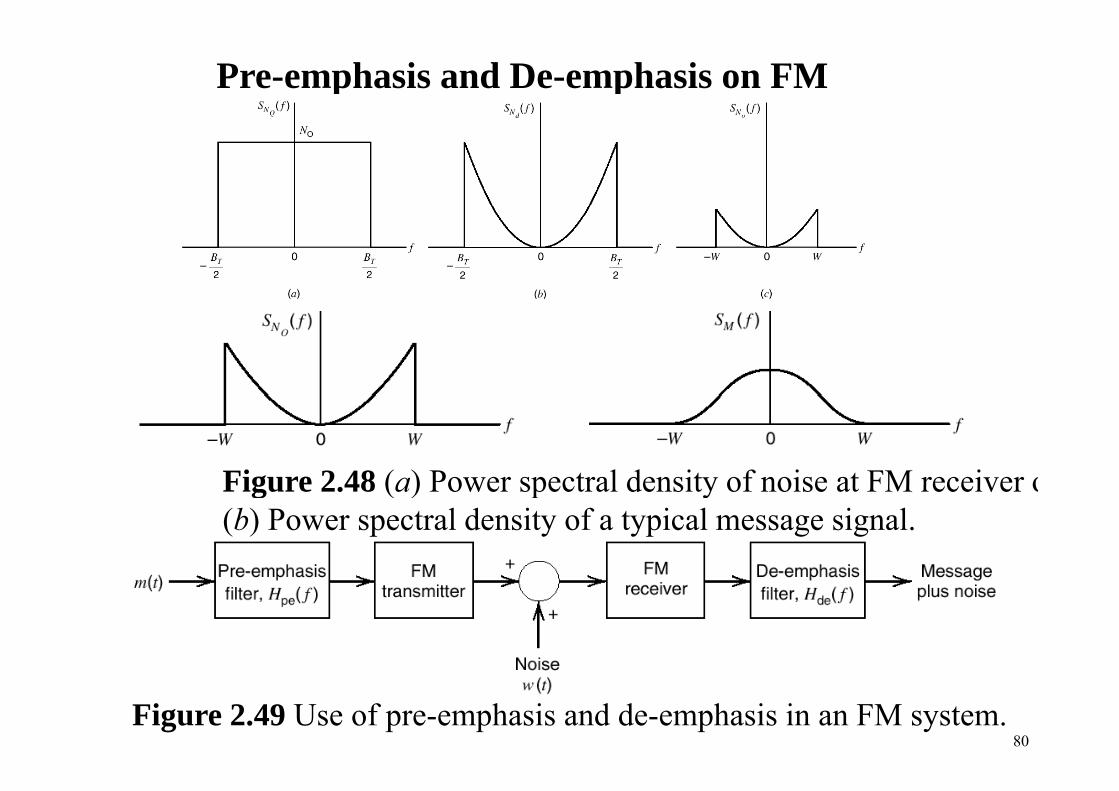
Pre-emphasis and De-emphasis on FM
Figure 2 48 (a) Power spectral density of noise at FM receiver oFigure 2.48 (a) Power spectral density of noise at FM receiver o(b) Power spectral density of a typical message signal.
Figure 2.49 Use of pre-emphasis and de-emphasis in an FM system.80
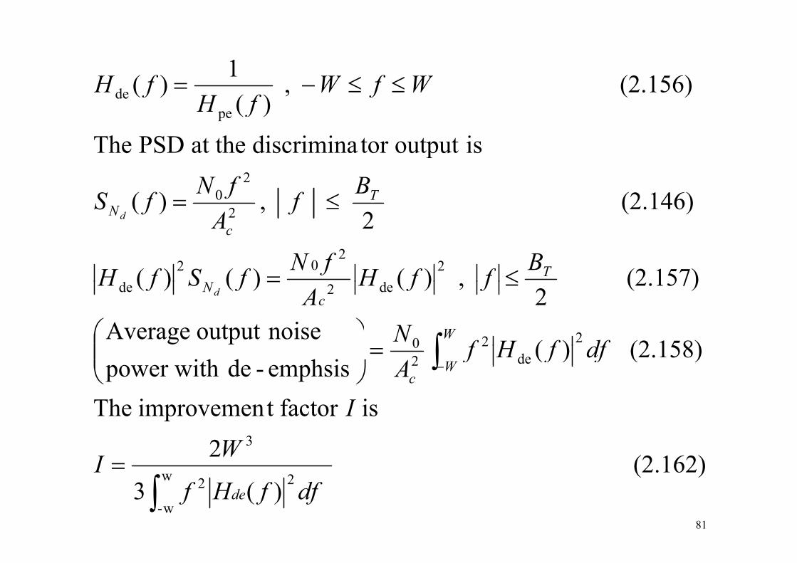
(2.156),1)(d ≤≤−= WfWfH
isoutput tor discriminaat the PSDThe
(2.156) , )(
)(pe
de ≤≤ WfWfH
fH
(2.146) 2
, )(
p
2
20 ≤=
BfA
fNfS TNd
(2 157))()()(
2
22
02 ≤=BffHfNfSfH
A
T
cd
(2 158))( noiseoutput Average
(2.157) 2
, )()()(
220
de2de
∫⎟⎟⎞
⎜⎜⎛
≤=
dffHfN
ffHA
fSfH
W
cNd
isfactortimprovemenThe
(2.158) )(emphsis-de power with de
220 ∫=⎟⎟
⎠⎜⎜⎝ −
I
dffHfA W
c
(2.162) 2isfactor t improvemenThe
3
=WI
I
( ) )(3
w
w-
22∫ dffHf de
81
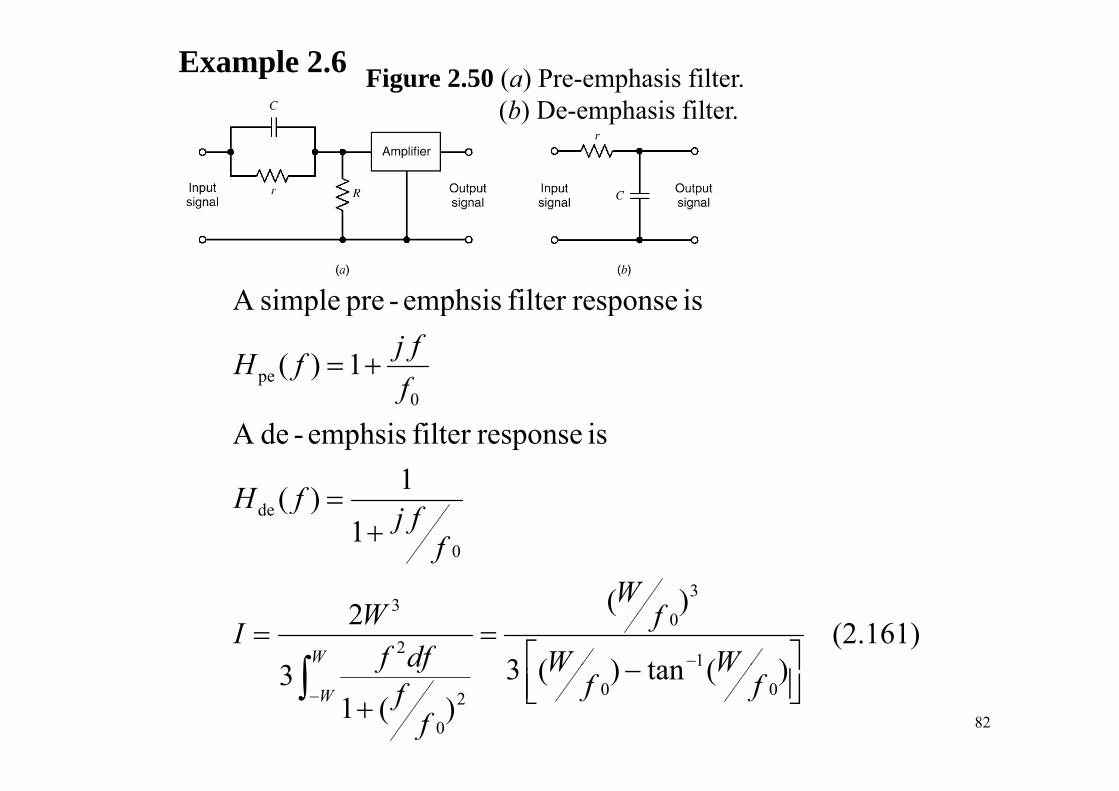
Example 2.6 Figure 2.50 (a) Pre-emphasis filter.(b) De-emphasis filter.
isresponsefilteremphsis-presimpleA
1)(
isresponsefilter emphsispresimpleA
0pe +=
fj ffH
1 is responsefilter emphsis-deA
0f
1
1)(0
de+
=
fj ffH
(2.161) )(t)(3
)(
3
21
3
0
2
3
⎤⎡==
−
∫ WWf
W
dffWI
W )(tan)(3)(1
3 0
1
02
0
⎥⎦⎤
⎢⎣⎡ −
+−∫ fW
fW
ffdff
W 82
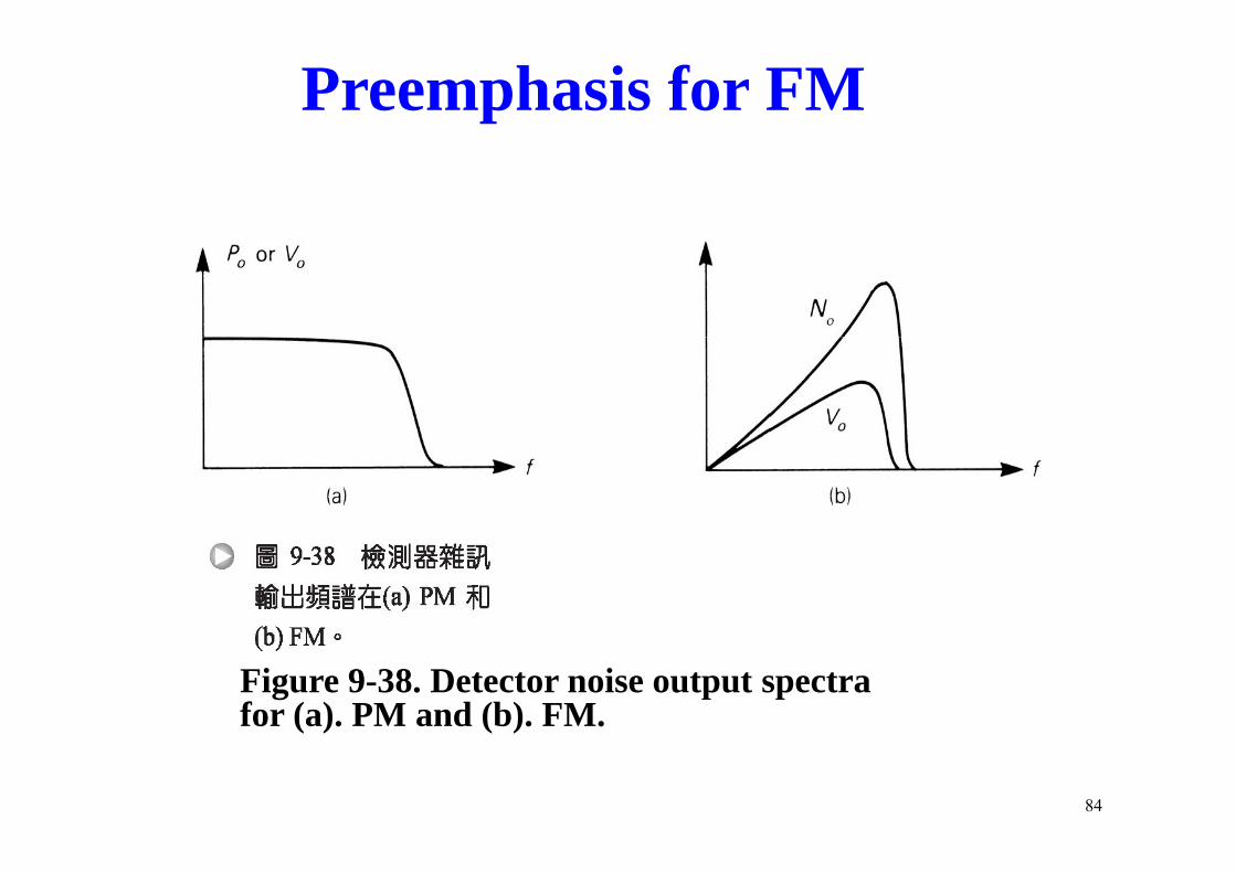
Preemphasis for FMThe main difference between FM and PM is in the relationship between frequency and phase.
f = (1/2π).dθ/dt. A PM detector has a flat noise power (and voltage) output
f ( t l d it ) Thi iversus frequency (power spectral density). This is illustrated in Figure 9-38a. However an FM detector has a parabolic noise powerHowever, an FM detector has a parabolic noise power spectrum, as shown in Figure 9-38b. The output noise voltage increases linearly with frequency.g y q yIf no compensation is used for FM, the higher audio signals would suffer a greater S/N degradation than the lower frequencies. For this reason compensation, called emphasis, is used for broadcast FM.
83
Preemphasis for FM
Figure 9-38. Detector noise output spectrafor (a). PM and (b). FM.
84
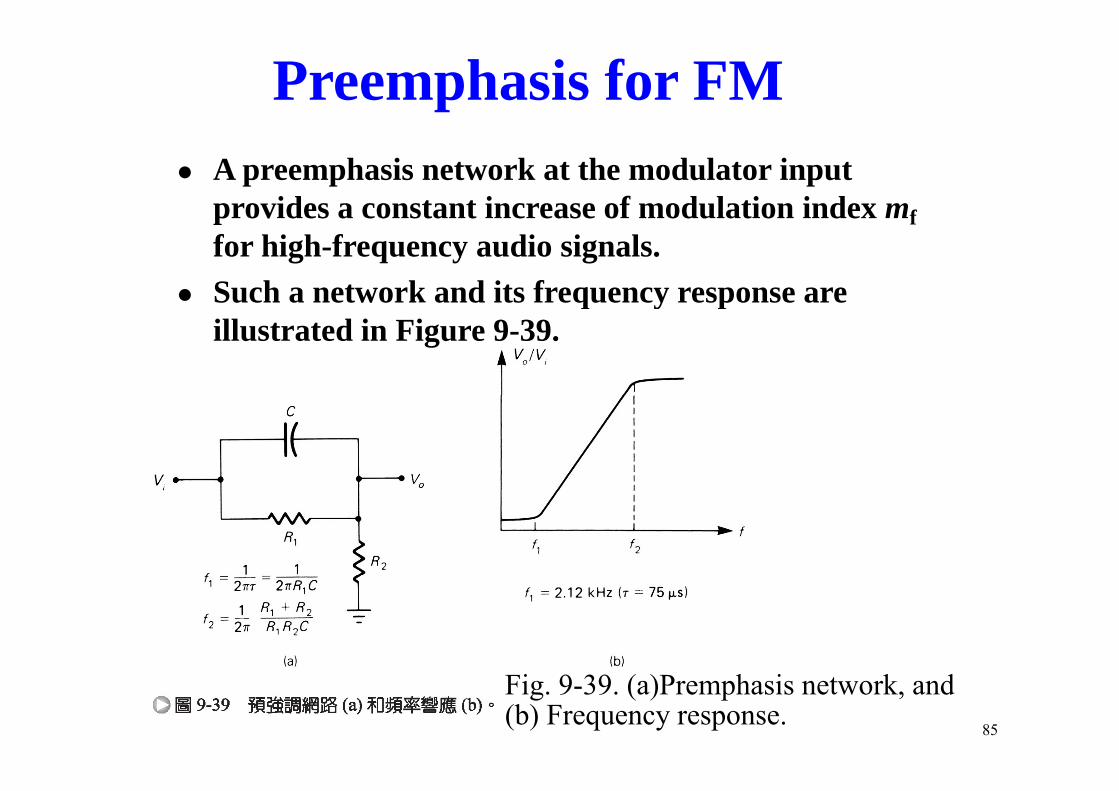
Preemphasis for FMA preemphasis network at the modulator input provides a constant increase of modulation index mfprovides a constant increase of modulation index mffor high-frequency audio signals. Such a network and its frequency response are q y pillustrated in Figure 9-39.
Fig. 9-39. (a)Premphasis network, and (b) Frequency response.
85
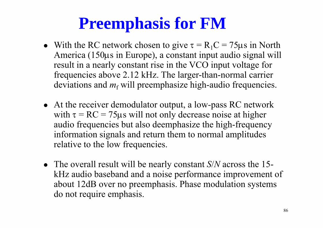
Preemphasis for FMWith the RC network chosen to give τ = R1C = 75μs in North America (150μs in Europe), a constant input audio signal will
lt i l t t i i th VCO i t lt fresult in a nearly constant rise in the VCO input voltage for frequencies above 2.12 kHz. The larger-than-normal carrier deviations and mf will preemphasize high-audio frequencies. f p p g q
At the receiver demodulator output, a low-pass RC network with τ = RC = 75μs will not only decrease noise at higherwith τ = RC = 75μs will not only decrease noise at higher audio frequencies but also deemphasize the high-frequency information signals and return them to normal amplitudes relative to the low frequencies.
The overall result will be nearly constant S/N across the 15-The overall result will be nearly constant S/N across the 15kHz audio baseband and a noise performance improvement of about 12dB over no preemphasis. Phase modulation systems d t i h ido not require emphasis.
86
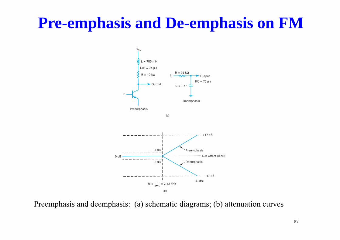
Pre-emphasis and De-emphasis on FM
P h i d d h i ( ) h ti di (b) tt tiPreemphasis and deemphasis: (a) schematic diagrams; (b) attenuation curves
87
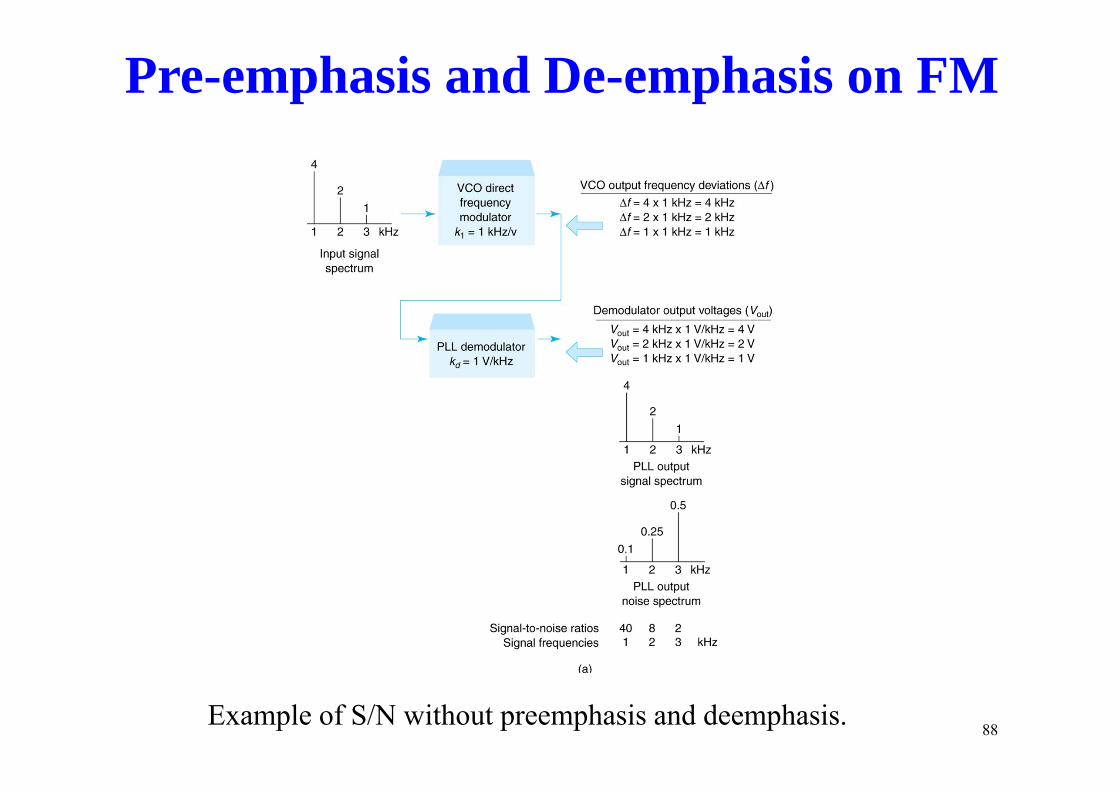
Pre-emphasis and De-emphasis on FM
Example of S/N without preemphasis and deemphasis. 88
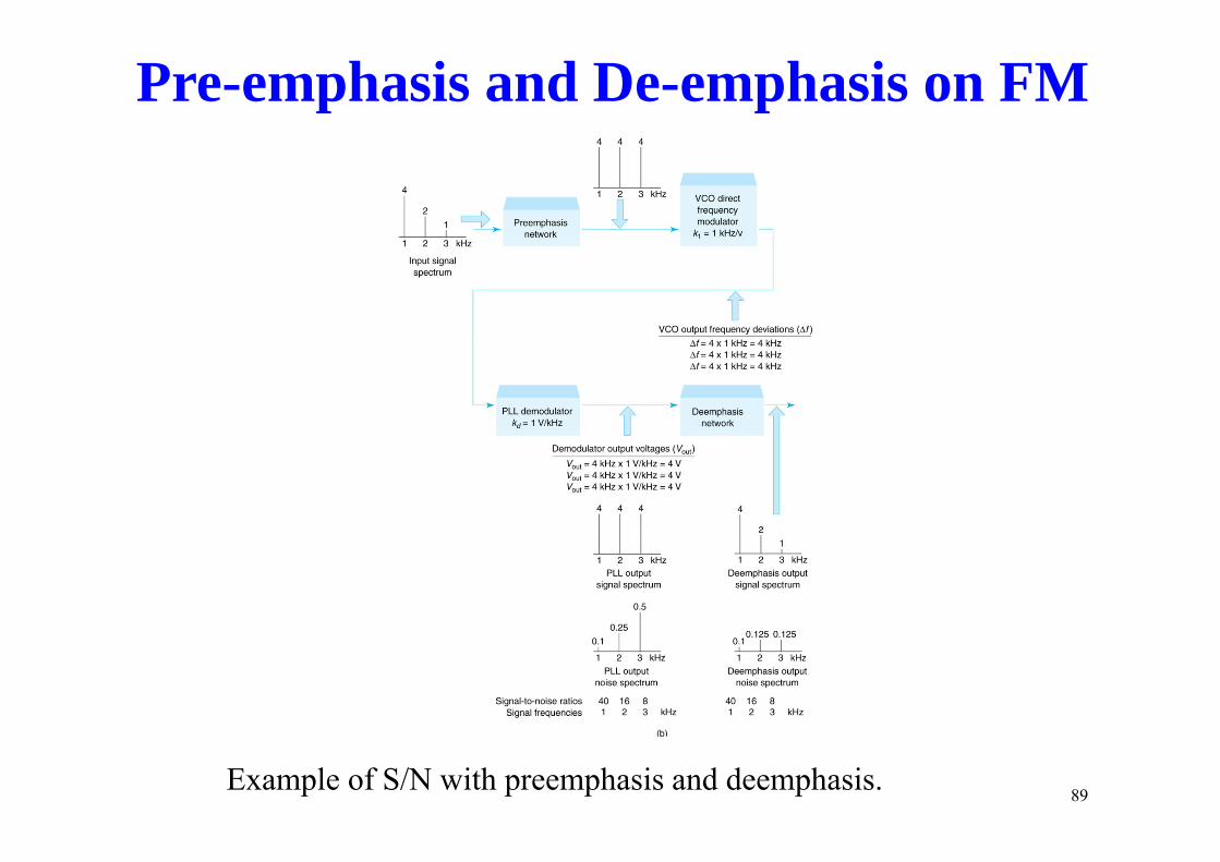
Pre-emphasis and De-emphasis on FM
Example of S/N with preemphasis and deemphasis. 89
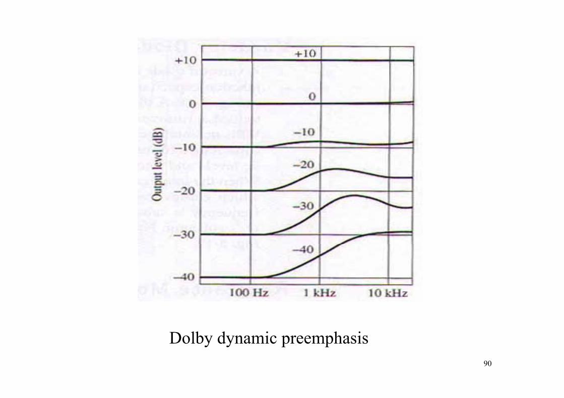
D lb d i h iDolby dynamic preemphasis90
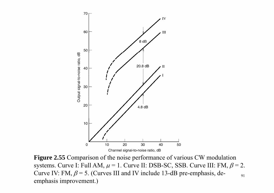
Figure 2.55 Comparison of the noise performance of various CW modulation systems. Curve I: Full AM, μ = 1. Curve II: DSB-SC, SSB. Curve III: FM, β = 2. Curve IV: FM, β = 5. (Curves III and IV include 13-dB pre-emphasis, de-emphasis improvement.)
91
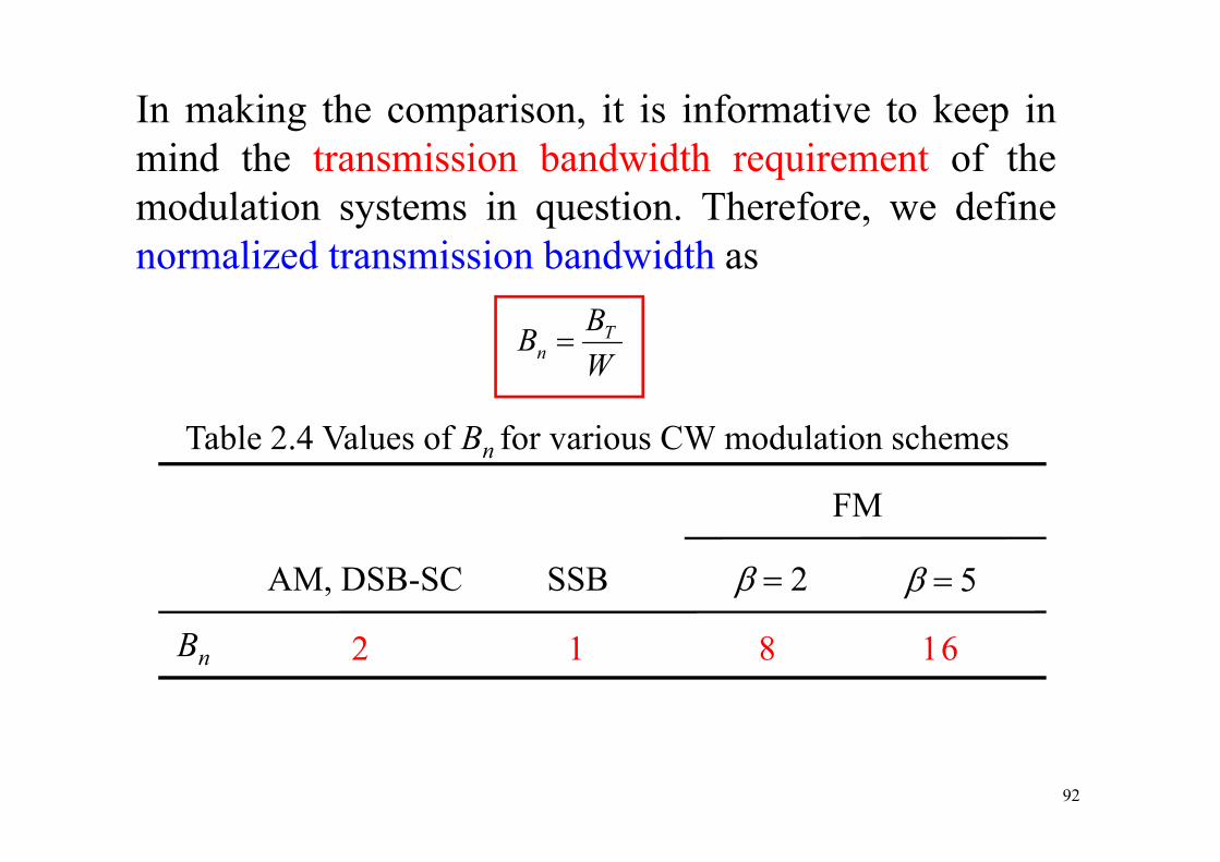
In making the comparison, it is informative to keep inmind the transmission bandwidth requirement of themodulation systems in question. Therefore, we definenormalized transmission bandwidth as
BB T
WB T
n =
T bl 2 4 V l f B f i CW d l ti hTable 2.4 Values of Bn for various CW modulation schemes
FM
AM, DSB-SC SSB β = 2 β = 5
Bn 2 1 8 16
92