z ;z ;:::;z - Annals of...
82
Annals of Mathematics 183 (2016), 95–176 http://dx.doi.org/10.4007/annals.2016.183.1.3 K¨ ahler–Einstein metrics with edge singularities By Thalia Jeffres, Rafe Mazzeo, and Yanir A. Rubinstein Abstract This article considers the existence and regularity of K¨ ahler–Einstein metrics on a compact K¨ ahler manifold M with edge singularities with cone angle 2πβ along a smooth divisor D. We prove existence of such metrics with negative, zero and some positive cases for all cone angles 2πβ ≤ 2π. The results in the positive case parallel those in the smooth case. We also establish that solutions of this problem are polyhomogeneous, i.e., have a complete asymptotic expansion with smooth coefficients along D for all 2πβ < 2π. 1. Introduction Let D ⊂ M be a smooth divisor in a compact K¨ ahler manifold. A K¨ ahler edge metric on M with angle 2πβ along D is a K¨ ahler metric on M \D that is asymptotically equivalent at D to the model edge metric g β := |z 1 | 2β-2 |dz 1 | 2 + n X j =2 |dz j | 2 ; here z 1 ,z 2 ,...,z n are holomorphic coordinates such that D = {z 1 =0} locally. We always assume that 0 <β ≤ 1. Of particular interest is the existence and geometry of metrics of this type that are also Einstein. The existence of K¨ ahler–Einstein (KE) edge metrics was first conjectured by Tian in the mid 1990’s [60]. In fact, Tian conjectured the existence of KE metrics with ‘crossing’ edge singularities when D has simple normal crossings. One motivation was his observation that these metrics could be used to prove various inequalities in algebraic geometry; in particular, the Bogomolov–Miyaoka–Yau inequality could be proved by deforming the cone angle of K¨ ahler–Einstein edge metrics with negative curvature to 2π. Further- more, these metrics can be used to bound the degree of immersed curves in gen- eral type varieties. He also anticipated that the complete Tian–Yau KE metric on the complement of a divisor should be the limit of the K¨ ahler–Einstein edge c 2016 Department of Mathematics, Princeton University. 95
-
Upload
nguyenquynh -
Category
Documents
-
view
215 -
download
0
Transcript of z ;z ;:::;z - Annals of...
Annals of Mathematics 183 (2016), 95–176http://dx.doi.org/10.4007/annals.2016.183.1.3
Kahler–Einstein metricswith edge singularities
By Thalia Jeffres, Rafe Mazzeo, and Yanir A. Rubinstein
Abstract
This article considers the existence and regularity of Kahler–Einstein
metrics on a compact Kahler manifold M with edge singularities with cone
angle 2πβ along a smooth divisor D. We prove existence of such metrics
with negative, zero and some positive cases for all cone angles 2πβ ≤ 2π.
The results in the positive case parallel those in the smooth case. We also
establish that solutions of this problem are polyhomogeneous, i.e., have
a complete asymptotic expansion with smooth coefficients along D for all
2πβ < 2π.
1. Introduction
Let D ⊂M be a smooth divisor in a compact Kahler manifold. A Kahler
edge metric on M with angle 2πβ along D is a Kahler metric on M\D that is
asymptotically equivalent at D to the model edge metric
gβ := |z1|2β−2|dz1|2 +n∑j=2
|dzj |2;
here z1, z2, . . . , zn are holomorphic coordinates such that D = z1 = 0 locally.
We always assume that 0 < β ≤ 1.
Of particular interest is the existence and geometry of metrics of this type
that are also Einstein. The existence of Kahler–Einstein (KE) edge metrics was
first conjectured by Tian in the mid 1990’s [60]. In fact, Tian conjectured the
existence of KE metrics with ‘crossing’ edge singularities when D has simple
normal crossings. One motivation was his observation that these metrics could
be used to prove various inequalities in algebraic geometry; in particular, the
Bogomolov–Miyaoka–Yau inequality could be proved by deforming the cone
angle of Kahler–Einstein edge metrics with negative curvature to 2π. Further-
more, these metrics can be used to bound the degree of immersed curves in gen-
eral type varieties. He also anticipated that the complete Tian–Yau KE metric
on the complement of a divisor should be the limit of the Kahler–Einstein edge
c© 2016 Department of Mathematics, Princeton University.
95
96 THALIA JEFFRES, RAFE MAZZEO, and YANIR A. RUBINSTEIN
metrics as the angle 2πβ tends to 0. Recently, Donaldson [24] proposed using
these metrics in a similar way to construct smooth Kahler–Einstein metrics on
Fano manifolds by deforming the cone angle of Kahler–Einstein metrics of pos-
itive curvature, and more generally to relate this approach to the much-studied
obstructions to existence of smooth Kahler–Einstein metrics.
One of the main results in this article is a proof of Tian’s conjecture on
the existence of Kahler–Einstein edge metrics when D is smooth. In a sequel
to this article we shall prove the general case [46]; this involves substantial
additional complications due to the singularities of the divisor.
In the lowest dimensional setting, M is a Riemann surface and the problem
is to find constant curvature metrics with prescribed conic singularities (with
cone angle less than 2π) at a finite collection of points. This was accomplished
in general by McOwen and Troyanov [49], [67]; as part of this, Troyanov found
some interesting restrictions on the cone angles necessary for the existence of
spherical cone metrics. Later, Luo and Tian [41] established the uniqueness of
these metrics. For the problem in higher dimensions, we focus only on the case
where D is smooth, unless explicitly stated. A preliminary study of the case of
Kahler–Einstein edge metrics with negative curvature appeared in the thesis
of the first named author [33], where it was already suggested that some of the
a priori estimates of Aubin and Yau [2], [70] should carry over to this setting
when β ∈ (0, 12 ]. An announcement for the existence in that negative case with
β ∈ (0, 12 ] was made over ten years ago by the first and second named authors
[45]. There were several analytic issues described in that announcement that
seemed to complicate the argument substantially, and details never appeared.
Recently there has been a renewed interest in these problems stemming
from an important advance by Donaldson [24], alluded to just above, whose
insightful observations make it possible to establish good linear estimates. He
proves a deformation theorem, showing that the set of attainable cone angles
for KE edge metrics is open. The key to his work is the identification of
a function space in the space of bounded functions on which the linearized
Monge–Ampere equation is solvable.
We realized, immediately following the appearance of [24], that the change
of perspective suggested by his advance makes it possible to apply the theory
of elliptic edge operators from [43] so as to circumvent the difficulties surround-
ing the openness part of the argument proposed in [45]. Indeed, we show that
estimates equivalent to those of Donaldson (but on slightly different function
spaces) follow from some of the basic results in that theory, and we explain
this at some length in this paper. This alternate approach to the linear the-
ory allows us to go somewhat further, and we use it to show that solutions
are polyhomogeneous, i.e., have complete asymptotic expansions in possibly
noninteger powers of the distance to the divisor and positive integer powers of
KAHLER–EINSTEIN METRICS WITH EDGE SINGULARITIES 97
the log of this distance function, with all coefficients smooth along the divisor.
This was announced in [45] and speculated on in [24], and the existence of this
higher regularity should be very helpful in the further study of these metrics.
What we achieve here is the following. We prove existence of Kahler–
Einstein edge (KEE) metrics with cone angle 2πβ that have negative, zero
and positive curvature, as appropriate, for all cone angles 2πβ ≤ 2π, when D
is smooth. Existence in the positive case is proved under the condition that
the twisted Mabuchi K-energy is proper, in parallel to Tian’s result in the
smooth case [61]. Next, we prove that solutions of a general class of complex
Monge–Ampere equations are polyhomogeneous, i.e., have complete asymp-
totic expansions with smooth coefficients. We provide a sharper identification
of the function space defined by Donaldson for his deformation result. As we
have briefly noted above, there are two slightly different scales of Holder spaces
that play a role in this type of problem. One, used in [24], we call the wedge
Holder spaces; the other, from [43], are the edge Holder spaces. Functions in
the wedge Holder spaces are slightly more regular, which is crucial in certain
parts of the argument; on the other hand, the edge Holder spaces are invariant
with respect to the dilation structure inherent in this problem, which makes
the linear theory, and certain parts of the nonlinear theory, more transparent.
We shall employ these spaces at various points in the argument. What
makes it possible to go from the edge spaces back to the wedge spaces is
Tian’s regularity argument from Appendix B, which shows that any solution
to the Monge–Ampere equation that is bounded along with its Laplacian is
automatically in a wedge Holder space. The results in Section 4 then show
that the solution is polyhomogeneous.
The key new ingredient for deriving the nonlinear a priori estimates is the
new Ricci continuity method, which can be considered as a continuity method
analogue of the Ricci flow. This was introduced in the context of the Ricci
iteration by the third named author [52], and one point of this article is to
show that it is perhaps the best suited for proving existence of Kahler–Einstein
metrics. Indeed, we derive our estimates also for more classical continuity paths
studied in the literature and at the appropriate junctures indicate how these
break down unless β is in the restricted “orbifold range” (0, 12 ], while this new
continuity method works for all β ∈ (0, 1].
In proving the a priori estimates we have made an effort to extend vari-
ous classical arguments and bounds to this singular setting with minimal as-
sumptions on the background geometry. In particular, the Ricci continuity
method together with the Chern–Lu inequality allows us to obtain the a pri-
ori estimate on the Laplacian assuming only that the reference edge metric
has bisectional curvature bounded above. We then explain how the Evans–
Krylov theory together with our asymptotic expansion imply a priori Holder
98 THALIA JEFFRES, RAFE MAZZEO, and YANIR A. RUBINSTEIN
bounds on the second derivatives for all cone angles with no further curvature
assumptions. Reducing the dependence of the estimates for the existence of a
Kahler–Einstein metric to only an upper bound on the bisectional curvature
of the reference metric does not seem to have been observed previously even
in the smooth setting, where traditionally a lower bound on the bisectional
curvature is required, or at least an upper bound on the bisectional curvature
together with a lower bound on some curvature. Thus, as a by-product, we
also obtain a new and unified proof of the classical results of Aubin, Yau and
Tian, on existence of KE metrics on smooth compact Kahler manifolds. Fi-
nally, in the case of positive curvature, we show how to control the Sobolev
constant and infimum of the Green function, which are both needed for the
uniform estimate. In an appendix it is shown that the bisectional curvature of
one reference metric is bounded from above on M\D whenever β ∈ (0, 1]. The
difficult calculations to establish this were obtained by the third named author
and Chi Li, and this appendix constitutes yet another necessary component of
this work.
Before stating our results, let us mention some other recent articles con-
cerning existence. It was expected that if one were to have linear estimates
such as the ones obtained by Donaldson [24], and if β ∈ (0, 12 ], so that the
curvature of the reference metric is bounded, then it should be possible to
adapt the classical Aubin–Yau a priori estimates and hence obtain existence
when µ ≤ 0. This was carried out in [15]. Another quite different approach
to existence for β ∈ (0, 12 ] and µ ≤ 0 but allowing divisors with simple normal
crossings, based on approximation by smooth metrics (and thus avoiding the
linear estimates), is due to Campana, Guenancia and Paun [16]. Both [15]
and [16] appeared around the same time as the present article. Finally, in
a different direction, Berman [9] showed how to bypass the linear estimates
and produce KE metrics whose volume form is asymptotic to that of an edge
metric using a variational approach. However, neither of these methods give
good information about the regularity or the geometry of the solution metric
near the divisor.
We now state our main results more precisely. Since some of the termi-
nology in these two theorems is perhaps unfamiliar in complex geometry, we
recall the notion of polyhomogeneity described briefly earlier in this introduc-
tion. The existence of a polyhomogeneous expansion should be regarded as an
optimal regularity statement for a solution, and it is the natural and unavoid-
able replacement for smoothness for these types of degenerate problems. Just
as with the Taylor expansions for smooth functions, the asymptotic expansions
we use in this paper are rarely convergent. We refer to Sections 2 and 3 for
more on this and for all relevant notation.
KAHLER–EINSTEIN METRICS WITH EDGE SINGULARITIES 99
Theorem 1 (Asymptotic expansion of solutions). Let ω be a polyhomo-
geneous Kahler edge metric with angle 2πβ ∈ (0, 2π]. Suppose that, for some
Holder exponent γ ∈ (0, 1), u ∈ D0,γs ∩ PSH(M,ω), s = w or e, is a solution
of the complex Monge–Ampere equation
(1) ωnu = ωnef−su, on M \D,
where ωu = ω+√−1 ∂∂u and f ∈ A0
phg(X). Then u is polyhomogeneous, i.e.,
u ∈ A0phg(X).
This result admits a straightforward generalization if the exponential on
the right-hand side is replaced by a function F (z, u) that is polyhomogeneous
in its arguments and is such that if u ∈ A0phg, then F (z, u) ∈ A0
phg.
Theorem 2 (Kahler–Einstein edge metrics). Let (M,ω0) be a compact
Kahler manifold with D⊂M a smooth divisor, and suppose µ[ω0]+(1− β)[D]
= c1(M), where β ∈ (0, 1] and µ ∈ R. If µ > 0, suppose in addition that
the twisted K-energy Eβ0 is proper. Then there exists a Kahler–Einstein edge
metric ωϕKE with Ricci curvature µ and with angle 2πβ along D. This metric
is unique when µ < 0, unique in its Kahler class when µ = 0 and unique up to
automorphisms that preserve D when µ > 0. This metric is polyhomogeneous ;
namely, ϕKE admits a complete asymptotic expansion with smooth coefficients
as r → 0 of the form
(2) ϕKE(r, θ, Z) ∼∑j,k≥0
Nj,k∑`=0
ajk`(θ, Z)rj+k/β(log r)`,
where r = |z1|β/β and θ = arg z1, and with each ajk` ∈ C∞. There are no
terms of the form rζ(log r)` with ` > 0 if ζ ≤ 2. In particular, ϕKE has infinite
conormal regularity and a precise Holder regularity as measured relative to the
reference edge metric ω, which is encoded by ϕKE ∈ A0 ∩ D0,γw .
We refer to Proposition 4.4 for the determination of the first several terms
in the expansion (2).
To clarify the conclusions about regularity in these theorems, we first
prove infinite ‘conormal’ regularity (ϕ ∈ A0), which means simply that the
solution is tangentially smooth and also infinitely differentiable with respect
to the vector field r∂r; we then establish Holder continuity of some second
derivatives with respect to the model metric (ϕ ∈ D0,γw ); finally, we prove
the existence of an asymptotic expansion in powers of the distance to the
edge (ϕ ∈ A0phg). This expansion also leads to the precise asymptotics of the
curvature tensor and its covariant derivatives. For example, when β ≤ 12 , we
have ϕKE ∈ C2, 1β−2
w , all third derivatives of the form (ϕKE)ijk belong to C0, 1β−2
w ,
and therefore so do all Christoffel symbols, and the curvature tensor of ωϕKE is
100 THALIA JEFFRES, RAFE MAZZEO, and YANIR A. RUBINSTEIN
Holder continuous. However, assuming only that β ≤ 1, we have ∆ωϕKE ∈ C0,γw
for some γ ∈ (0, 1β − 1], but in general the curvature tensor does not lie in L∞.
(This follows readily from the calculations of the appendix.) Again, we refer
to Proposition 4.4 for more precise information.
Theorem 2 is the generalization to the edge setting of the classical the-
orems of Aubin, Yau (µ ≤ 0) and Tian (µ > 0) on existence of KE metrics
in the compact smooth setting [2], [70], [61]. Its proof gives a new and uni-
fied treatment for all µ even in the smooth setting. It is also a satisfactory
generalization of Troyanov’s theorem on the existence of constant curvature
metrics with conic singularities on Riemann surfaces [67] inasmuch as the cone
angle restrictions that appear in his work arise only in the positive curvature
case, and they are the same as the properness of the twisted K-energy in that
setting. Just as for the smooth setting [61], the properness assumption should
be a necessary condition for existence in the absence of holomorphic vector
fields that are tangent to D.
Finally, consider the special case that M is Fano and D is a smooth
anticanonical divisor. (The existence of such a divisor is related to the so-
called Elephant Conjectures in algebraic geometry and is known when n ≤ 3
by work of Shokurov and others.) Then, as noted by Berman [9], the twisted
K-energy is proper for small µ = β. Theorem 2 thus gives the following
corollary conjectured by Donaldson [23].
Corollary 1. Let M be a Fano manifold, and suppose that there exists
a smooth anticanonical divisor D ⊂ M . Then there exists some β0 ∈ (0, 1]
such that for all β ∈ (0, β0), there exists a KEE metric with angle 2πβ along
D and with positive Ricci curvature equal to β.
Added in revision : There has been substantial work in this area in the
years following the initial appearance of this article; cf., in particular, the
papers [22], [51], [17], [18], [19], [63]. We refer the reader to the survey [53]
for further references and background. In both [18] and [63], the construction
of a smooth KE metric is carried out by studying the deformations of a KEE
metric as the cone angle increases.
Our original proof of the D0,γw estimate had an error, now corrected by
Appendix B. The paper [18] contains a different approach to this estimate.
Acknowledgements. The authors are grateful to Gang Tian for his advice
and encouragement throughout the course of this project and also for explain-
ing to us his argument that appears in Appendix B. Various referees made
numerous valuable remarks that led to a better exposition and that drew our
attention to errors, some rather important, in earlier versions. The authors
also offer many thanks to Simon Donaldson for his interest in this work and
KAHLER–EINSTEIN METRICS WITH EDGE SINGULARITIES 101
for numerous comments that helped sharpen, clarify and in some instances
correct the exposition. The NSF supported this research through grants DMS-
0805529, 1105050 (R.M.) and DMS-0802923, 1206284 (Y.A.R.).
2. Preliminaries
We set the stage for the rest of the article with a collection of facts and
results needed later. First consider the flat model situation, where M = Cnwith linear coordinates (z1, . . . , zn) and D is the linear subspace z1 = 0. For
brevity we often write
Z = (z2, . . . , zn).
The model singular Kahler form and singular Kahler metric are given by
ωβ =1
2
√−1
Ç|z1|2β−2dz1 ∧ dz1 +
n∑j=2
dzj ∧ dzjå
(3)
and
gβ = |z1|2β−2|dz1|2 +n∑j=2
|dzj |2.(4)
This is the product of a flat one complex dimensional conic metric with cone
angle 2πβ with Cn−1. We always assume that 0 < β ≤ 1; the expressions
above make sense for any real β, but their geometries are quite different for β
outside of this range.
Now suppose that M is a compact Kahler manifold and D a smooth
divisor. Fix β ∈ (0, 1] and µ ∈ R, and assume that there is a Kahler class
Ω = Ωµ,β such that
(5) µΩ + 2π(1− β)c1(LD) = 2πc1(M).
Here, LD is the line bundle associated to D. Thus, c1(M)− (1− β)c1(LD) is
a positive or negative class if µ > 0 or µ < 0. If µ = 0, then Ω is an arbitrary
Kahler class.
Let g be any Kahler metric that is smooth (or of some fixed finite regular-
ity) on M \D. We shall say that g is a Kahler edge metric with angle 2πβ if,
in any local holomorphic coordinate system near D where D = z1 = 0 and
z1 = ρe√−1θ,
(6) g11 = Fρ2β−2, g1 = gi1 = O(ρβ−1+η′), and all other gi = O(1),
for some η′ > 0, where F is a bounded nonvanishing function that is at least
continuous at D (and that will have some specified regularity). If this is the
case, we say that g is asymptotically equivalent to gβ and that its associated
Kahler form ω (which by abuse of terminology we sometimes also refer to
as a metric) is asymptotically equivalent to ωβ. There are slightly weaker
hypotheses under which it is reasonable to say that g has angle 2πβ at D, but

102 THALIA JEFFRES, RAFE MAZZEO, and YANIR A. RUBINSTEIN
the definition we have given here is sufficient for our purposes. We denote by
Ricω the Ricci current (on M) associated to ω, namely, in local coordinates
Ricω = −√−1∂∂ log det[gij ] if ω =
√−1gijdz
i∧dzj . Thus, Ricω−2π(1−β)[D]
is a (1, 1) current on M with a continuous potential, where [D] is the current
associated to integration along D.
Definition 2.1. With all notation as above, a Kahler current ω, with as-
sociated singular Kahler metric g, is called a Kahler–Einstein edge current,
respectively metric, with angle 2πβ along D and Ricci curvature µ if ω and g
are asymptotically equivalent to ωβ and gβ and if
(7) Ricω − 2π(1− β)[D] = µω.
In this section we present some preliminary facts about the geometry and
analysis of the class of Kahler edge metrics. We first review some different co-
ordinate charts near the edge D used extensively below. Many calculations in
this article are most easily done in a singular real coordinate chart, although
when the complex structure is particularly relevant to a calculation, we use
certain adapted complex coordinate charts. While all of this is quite elemen-
tary, there are some identifications that can be confusing, so it is helpful to
make all of this very explicit. We calculate the curvature tensor for any one
such metric g, assuming it is sufficiently regular. We then introduce the rele-
vant class of Kahler edge potentials and describe the continuity method that
will be used for the existence theory. As we recall, this particular continuity
method is closely related to the Ricci iteration that, naturally, we also treat
simultaneously in this article. We conclude the section with a fairly lengthy
description of the various function spaces that will be used later. Rather than
a purely technical matter, this discussion gets to the heart of some of the more
important analytic and geometric issues that must be faced here. There are
two rather different choices of Holder spaces; one is naturally associated to this
class of Kahler edge metrics and was employed, albeit in a slightly different
guise, by Donaldson [24], while the other, from [43], is well adapted to this
edge geometry because of its naturality under dilations and has been used in
many other analytic and geometric problems where edges appear. Use of these
latter function spaces is central to our method.
2.1. Coordinate systems. Fix local complex coordinates (z1, . . . , zn) =
(z1, Z) with D = z1 = 0 locally. There are two other coordinate systems that
are quite useful for certain purposes. The first is a singular holomorphic coordi-
nate chart, where we replace z1 by ζ = zβ1 /β. Of course, ζ is multi-valued, but
we can work locally in the logarithmic Riemann surface that uniformizes this
variable. Thus if z1 = ρe√−1θ, then ζ = re
√−1θ, where r = ρβ/β and θ = βθ.
The second is the real cylindrical coordinate system (r, θ, y) around D, where
KAHLER–EINSTEIN METRICS WITH EDGE SINGULARITIES 103
r = |ζ| as above, θ is the argument of z1, and (y1, . . . , y2n−2) = (ReZ, ImZ).
Note that re√−1θ = z1|z1|β−1/β. We use either (z1, Z) or (ζ, Z) in situations
where the formalism of complex analysis is useful, and (r, θ, y) elsewhere. For
later purposes, note that
(8) dζ = zβ−11 dz1 ⇔ dz1 = (βζ)
1β−1dζ,
∂ζ
∂z1= zβ−1
1 ⇔ ∂z1
∂ζ= (βζ)
1β−1.
One big advantage of either of these other coordinate systems is that they
make the model metric gβ appear less singular. Indeed,
(9) gβ = |dζ|2 + |dZ|2 = dr2 + β2r2dθ2 + |dy|2.
In either case, one may regard the coordinate change as encoding the singu-
larity of the metric via a singular coordinate system. This is only possible for
edges of real codimension two, and there are many places, both in [24] and
here, where we take advantage of this special situation. For edges of higher
codimension, one cannot conceal the singular geometry so easily; see [43]. The
expression for gβ in cylindrical coordinates makes clear that for any β, β′, we
have C1gβ ≤ gβ′ ≤ C2gβ; the corresponding inequality in the original z co-
ordinates must be stated slightly differently, as C1gβ ≤ Φ∗gβ′ ≤ C2gβ, where
Φ(z1, . . . , zn) = (zβ′/β1 , z2, . . . , zn).
We now compute the complex derivatives in these coordinates. We have
∂z1 =1
2e−√−1θ
Ç∂ρ −
√−1
ρ∂θ
å=
1
2e−√−1θ(βr)
1− 1β
Ç∂r −
√−1
βr∂θ
å,(10)
and then
(11) ∂2z1z1 = (βr)
2− 2β
Å∂2r +
1
r∂r +
1
β2r2∂2θ
ã.
The other mixed complex partials ∂2z1zj
, ∂2ziz1
and ∂2zizj
are compositions of the
operator in (10) and its conjugate and certain combinations of the ∂y` . From
this we obtain that
(12) ∆gβu =n∑
i,j=1
(gβ)iui =
Å∂2r +
1
r∂r +
1
β2r2∂2θ + ∆y
ãu,
since (gβ)11 = ρ2−2β = (βr)2β−2
and (gβ)1, (gβ)i1 = 0 and all other (gβ)i = δij .
As already described, we shall work with the class of Kahler metrics g
that satisfy condition (6), and which we call asymptotically equivalent to gβ.
If g is of this type, then
(13) g11 = F−1ρ2−2β, g1, gi1 = O(ρη′+1−β), and all other gi = O(1)
104 THALIA JEFFRES, RAFE MAZZEO, and YANIR A. RUBINSTEIN
for some η′ > 0, hence
(14) ∆g = F−1
Ñ∂2r +
1
r∂r +
1
β2r2∂2θ +
2n−2∑r,s=1
crs(r, θ, y)∂2yrys
é+ E,
where
E := rη−2∑
i+j+|µ|≤2
aijµ(r, θ, y)(r∂r)i∂jθ(r∂y)
µ.
Here η > 0 is determined from η′ and β, and all coefficients have some specified
regularity down to r = 0. In particular, the coefficient matrix (crs) is positive
definite, with crs(0, θ, y) independent of θ, and the coefficients aijµ are bounded
as r → 0. Thus there are no cross-terms to leading order, and the 11 part of
the operator ∆g is ‘standard’ once we multiply the entire operator by F .
One way that this asymptotic structure will be used is as follows. Fun-
damental to this work is the role of the family of dilations Sλ : (r, θ, y) 7→(λr, θ, λy) centered at some point p ∈ D corresponding to y = 0. If we push
forward this operator by Sλ, which has the effect of expanding a very small
neighbourhood of p, then the principal part scales approximately like λ2 while
E scales like λ2−η. Hence, after a linear change of the y coordinates,
(15) Aλ−2(Sλ)∗∆g −→ ∆gβ as λ→∞,
where A = F (p). In particular, E scales away completely in this limit.
One important comment is that if the derivatives ui are all bounded, and
if g satisfies these asymptotic conditions, then so does g, where gi = gi + ui.
A key point in the treatment below, exploited by Donaldson [24], is that
for any Kahler metric g, ∆g only involves combinations of the following second-
order operators:
P11 =
Å∂2r +
1
r∂r +
1
β2r2∂2θ
ã,
P1¯=
Ç∂r −
√−1
βr∂θ
å∂z` ,
P`1 =
Ç∂r +
√−1
βr∂θ
å∂z` , ` = 2, . . . , n, and
P`k = ∂2z`zk
, `, k = 2, . . . , n.
Regularity properties in certain function spaces considered below involve pre-
cisely these derivatives, while others are less sensitive about the decomposition
of ∂zj and ∂zj into their (1, 0) and (0, 1) parts. We therefore introduce the
following collections of differential operators:
(16)Q = ∂r, r−1∂θ, ∂y` , ∂
2ry`, ∂2rθ, ∂
2θy`,
Q∗ = Qt ∂2yky`
, P11.
KAHLER–EINSTEIN METRICS WITH EDGE SINGULARITIES 105
The reason for singling out the extra operators in Q∗ \ Q is that the relevant
boundedness properties are more subtle for these.
As a final note, let us record the form of the complex Monge–Ampere
operator in these coordinates for any Kahler metric that satisfies the decay
assumptions above. We have
(ω +√−1 ∂∂u)n/ωn =
det(gi +√−1ui)
det gi= det(δji +
√−1uji ),
where uji = uikgjk. Using the calculations above, we have
u 11 =F−1P11u+O(rη)u1,
u j1 = e−
√−1 θ(βr)
1− 1β gjkP1ku+O(r
η+ 1β−1
)P11u,
u 1i =F−1e
√−1 θ(βr)
1β−1Pi1u+O(r
η+ 1β−1
)ui,
u ji = gjkPiku+O(rη)ui1.
This means that if we multiply every column but the first in (δ ji +
√−1u j
i )
by e√−1θ(βr)1/β−1 and every row but the first by e−
√−1θ(βr)1−1/β, then the
determinant remains the same, and we have shown that
(17)
det(gi +√−1ui)
det gi= det
Ü1 + F−1P11 u F−1P21 u . . . F−1Pn1u
......
......
gnkP1ku . . . . . . 1 + gn¯Pn¯u
ê+R,
where R = rηR0(upq), with R0 polynomial in its entries.
2.2. Kahler edge potentials. Fix a smooth Kahler form ω0 with [ω0] ∈ Ω ≡Ωµ,β. Consider the space of all Kahler potentials relative to ω0, asymptotically
equivalent to the model metric,
(18) Hω0 := ϕ ∈ C∞(M \D) ∩ C0(M) : ωϕ := ω0 +√−1∂∂ϕ > 0 on M
and ωϕ asymptotically equivalent to ωβ.
Note that in our notation, Hω0∼= Hη for any smooth η cohomologous to ω0 but
not for any η ∈ Hω0 . The first observation is that such Kahler edge metrics
exist.
Lemma 2.2. Let β ∈ (0, 1]. Then Hω0 is nonempty.
Proof. Let h be a smooth Hermitian metric on LD, and let s be a global
holomorphic section of LD so that D = s−1(0). We claim that for c > 0
sufficiently small, the function
(19) φ0 := c|s|2βh = c(|s|2h)β
106 THALIA JEFFRES, RAFE MAZZEO, and YANIR A. RUBINSTEIN
belongs to Hω0 . To prove this, it suffices to consider p ∈ M \D near D. Use
a local holomorphic frame e for LD and local holomorphic coordinates zini=1
valid in a neighborhood of p, such that s = z1e, so that locally D is cut out by
z1. Let
(20) a := |e|2h,
and set H := aβ, so |s|2βh = H|z1|2β. Note that H is smooth and positive.
Then
(21)
√−1 ∂∂|s|2βh = β2H|z1|2β−2
√−1 dz1 ∧ dz1
+ 2βRe(|z1|2βz1−1√−1 dz1 ∧ ∂H) + |z1|2β
√−1 ∂∂H.
For c > 0 small, the form ω0 +√−1∂∂φ0 is positive definite and satisfies the
conditions of (6) and hence is asymptotically equivalent to gβ.
It is useful to record the form of ωφ0 in the (ζ, Z) coordinates as well.
First note that if ψ0 is a Kahler potential for ω0, then using (8),
(22)
√−1 ∂∂ψ0 = (ψ0)z1z1 |βζ|
2β−2√−1 dζ ∧ dζ
+∑j>1
2Re((ψ0)z1zj (βζ)1β−1√−1 dζ ∧ dzj)
+∑i,j>1
(ψ0)zizj√−1 dzi ∧ dzj .
Next, |s|2βh = β2H|ζ|2, hence
(23)√−1 ∂∂(c|s|2βh ) = cβ2
Ä√−1Hdζ ∧ dζ + 2Re(ζ
√−1 dζ ∧ ∂H) + |ζ|2
√−1 ∂∂H
ä.
From these two expressions, it is clear once again that φ0 ∈ Hω0 when c is
sufficiently small. Putting these expressions together shows that ω0+√−1 ∂∂φ0
is locally equal to
(24)(|βζ|
2β−2
(ψ0)z1z1 + cβ2H + c|βζ|2βHz1z1 + 2cβ
1β
+1Re(ζ
1βHz1)
)√−1 dζ ∧ dζ
+ 2Re∑j>1
((βζ)
1β−1
(ψ0)z1zj + cβ2ζHzj
+ cβ1β
+1ζ
1β ζH
z1zj
)√−1 dζ ∧ dzj
+√−1 ∂Z ∂Zψ0 + |ζ|2
√−1 ∂Z ∂ZH.
The reason for writing the derivatives of ψ0 and H with respect to z1 rather
than ζ is because we know that both of these functions are smooth in the
original z coordinates, and hence so are its derivatives with respect to z.
We now use this expression to deduce some properties of the curvature
tensor of g. This turns out to be simple in this singular holomorphic coordinate
KAHLER–EINSTEIN METRICS WITH EDGE SINGULARITIES 107
system. The coefficients of the (0, 4) curvature tensor are given by
(25) Rikl = −gi,kl + gst git,k gsj,l,
where the indices after a comma indicate differentiation with respect to a
variable. In the following, contrary to previous notation, we temporarily use
the subscripts 1 and 1 to denote components of the metric or derivatives with
respect to ζ and ζ, not z1 or z1.
Lemma 2.3. The curvature tensor of ω = ω0 +√−1 ∂∂φ0 is uniformly
bounded on M \D provided β ∈ (0, 12 ].
Proof. Since in the (ζ, Z) coordinates, cI < [gi] < CI, it suffices to show
that |Rikl| < C. From (24),
g11,1 = O(|ζ|
2β−3),
g11,k = O(1),
g1,1 = O(|ζ|
1β−2),
g1,k = O(|ζ|+ |ζ|
1β−1),
gi,1 = O(|ζ|
1β−1),
gi,k = O(1).
Similarly, |gi,kl| ≤ C(1 + |ζ|
1β−2
+ |ζ|2β−4).
As conjectured by Donaldson, there seem to be genuine cohomological
obstructions to finding reference edge metrics with bounded curvature when
β > 1/2. Nevertheless, in Proposition A.1 it is shown that the bisectional
curvature of ω is bounded from above on M\D provided β ≤ 1. This fact comes
out of the proof as some kind of miracle, yet it would be enlightening to have a
more geometric explanation for it. In a related vein, we remark in passing that
it is not difficult to write down local expressions (near D) for metrics equivalent
to the model metric that have bisectional curvature unbounded from above or
below or both. For instance, when n = 1, the curvature of (|z1|2β−2 − 1)|dz1|2equals (1 − β)2ρ−2β/(1 − ρ2−2β)2 (here ρ = |z1|) and hence tends to +∞as ρ 0. More generally, one can easily choose ψ polyhomogeneous but
not smooth so that the curvature of the metric |z1|2β−2eψ|dz1|2 is unbounded,
either above or below or both. In other words, the asymptotics of the curvature
depend on the higher order terms in the expansion of the metric.
2.3. The twisted Ricci potential. From now on (except when otherwise
stated) we denote
(26) ω := ω0 +√−1 ∂∂φ0 ∈ Hω0 ,
with φ0 given by (19). In the remainder of this article, we refer to ω as the
reference metric. Define fω by
(27)√−1∂∂fω = Ricω − 2π(1− β)[D]− µω,
108 THALIA JEFFRES, RAFE MAZZEO, and YANIR A. RUBINSTEIN
where [D] denotes the current of integration along D, and with the normaliza-
tion
(28)1
V
∫Mefωωn = 1, where V :=
∫Mωn.
We call this the twisted Ricci potential (see Lemma 4.5 for precise regular-
ity of fω); this terminology refers to the fact that the adjoint bundle KM +
(1− β)LD takes the place of the canonical bundle KM . Alternatively, one can
also think of Ricω − 2π(1− β)[D] as a kind of Bakry-Emery Ricci tensor.
2.4. The Ricci continuity method for the twisted Kahler–Einstein equation.
The existence of Kahler–Einstein metrics asymptotically equivalent to gβ is
governed by the Monge–Ampere equation
(29) ωnϕ = efω−µϕωn.
We seek a solution ϕ ∈ Hω0 , and we shall do so using a particular continuity
method. We consider a continuity path in the space of metrics Hω (with
some specified regularity) obtained from the Ricci flow via a backwards Euler
discretization, as first suggested in [52]. Alternatively, it can be obtained
essentially by concatenating (and extending) two previously studied paths,
one by Aubin [3] in the positive case and the other by Tian–Yau [65] in the
negative case. The path is given by
(30) ωnϕ = ωnefω−sϕ, s ∈ (−∞, µ],
where ϕ(−∞) = 0 and ωϕ(−∞) = ω. We call this the Ricci continuity path.
Adapting the proof of a result of Wu [68], we prove later that there exists a
solution ϕ(s) for s −1 of the form s−1fω + o(1/s). A key feature of this
continuity path is that
(31) Ricωϕ = sωϕ + (µ− s)ω + 2π(1− β)[D],
which implies the very useful property that for all solutions ϕ(s) along this
path, the Ricci curvature is bounded below on M \D, i.e., Ricωϕ > sωϕ. As
we explain in Section 6.3, another important property is that the Mabuchi
K-energy is monotone along this path.
Much of the remainder of this article is directed toward analyzing this
family of Monge–Ampere equations: Section 3 describes the linear analysis
needed to understand the openness part of the continuity argument as well as
the regularity theory; Section 4 uses this linear analysis to prove that solutions
are automatically ‘smooth’ at D, by which we mean that they are polyhomo-
geneous (see below); the a priori estimates needed to obtain the closedness of
the continuity argument are derived in the remaining sections of the article,
and the proof is concluded in Section 9.
KAHLER–EINSTEIN METRICS WITH EDGE SINGULARITIES 109
We will pursue a somewhat parallel development of this proof using two
different scales of Holder spaces since we hope to illustrate the relative merits
of each of these classes of function spaces, with future applications in mind.
Certain aspects of the proof work much more easily in one setting rather than
the other, but we give a complete proof of the a priori estimates in either frame-
work. The proof of higher regularity, which shows that these two approaches
are ultimately equivalent and facilitates the continuity argument, relies directly
on only one of these scales of spaces.
Remark 2.4. The continuity path (30) has several useful properties, some
already noted above, which are necessary for the proof of Theorem 2 when
β > 1/2. However, we also consider the two-parameter family of equations
(32) ωnϕ = etfω+ct−sϕωn, ct := − log1
V
∫Metfωωn, (s, t) ∈ A,
where A := (−∞, 0] × [0, 1] ∪ [0, µ] × 1. This incorporates the continuity
path s = µ, 0 ≤ t ≤ 1, which is the common one in the literature. The analysis
required to study this two-parameter family requires little extra effort and has
been included since it may be useful elsewhere. It provides an opportunity to
use the Chern–Lu inequality in its full generality (see Section 7). In addition,
we have already noted that one cannot obtain openness for (30) at s = −∞ di-
rectly but must produce a solution for s (very) negative by some other method.
Wu [68] accomplishes this by a perturbation argument; the augmented conti-
nuity path (32) gives yet another means to do this, but it works only when
β ≤ 1/2. We refer to Section 9 for more details.
We emphasize that our proof of Theorem 2 when β > 1/2 or when µ > 0
requires the path (30) (i.e., fixing t = 1).
2.5. The twisted Ricci iteration. The idea of using the particular conti-
nuity method (30) to prove the existence of Kahler–Einstein metrics for all µ
(independently of sign) was suggested in [52, p. 1533]. As explained there and
recalled below, this path arises from discretizing the Ricci flow via the Ricci
iteration. After treating this continuity path we will be in a position to prove
smooth edge convergence of the (twisted) Ricci iteration to the Kahler–Einstein
edge metric.
One Kahler–Ricci flow in our setting is
∂ω(t)
∂t= −Ric ω(t) + 2π(1− β)[D] + µω(t), ω(0) = ω ∈ Hω0 .
Let τ ∈ (0,∞). The (time τ) Ricci iteration, introduced in [52], is the sequence
ωkτk∈N ⊂ Hω, satisfying the equations
ωkτ = ω(k−1)τ + τµωkτ − τRicωkτ + τ2π(1− β)[D], ω0τ = ω,
110 THALIA JEFFRES, RAFE MAZZEO, and YANIR A. RUBINSTEIN
for each k ∈ N for which a solution exists in Hω. This is the backwards Euler
discretization of the Kahler–Ricci flow. Equivalently, let ωkτ = ωψkτ , with
ψkτ =∑kl=1 ϕlτ . Then,
(33) ωnψkτ = ωnefω−µψkτ+ 1τϕkτ .
Since the first step is simply ωnϕτ = ωnefω+( 1τ−µ)ϕτ , the Ricci iteration exists
(uniquely) once a solution exists (uniquely) for (30) for s = µ − 1τ . Thus,
much like for the Ricci flow, a key point is to prove uniformity of the a priori
estimates as k tends to infinity. The convergence to the Kahler–Einstein metric
then follows essentially by the monotonicity of the twisted K-energy if the
Kahler–Einstein metric is unique.
As noted above, our choice of the particular continuity path (30) allows
us to treat the continuity method and the Ricci iteration in a unified manner.
When µ ≤ 0, our estimates for (30), the arguments of [52] and the higher regu-
larity developed in Section 4 imply the uniqueness, existence and edge smooth
convergence of the iteration for all τ . When µ > 0, the uniqueness of the
(twisted) Ricci iteration was proven recently by Berndtsson [12], and it follows
from his result that whenever the twisted K-energy Eβ0 is proper, then also
the Kahler–Einstein edge metric must be unique. Given this, our analysis here
and in [52] immediately implies smooth (in the edge spaces) convergence of the
iteration for large enough times steps, more specifically, provided τ > 1/µ and
Eβ0 is proper, or else provided τ > 1/αΩ,ω, and αΩ,ω > µ, where αΩ,ω is Tian’s
invariant defined in Section 6.3. (Note that by Lemma 6.11 this assumption
implies Eβ0 is proper.) As pointed out to us by Berman, given the results of
[52], the remaining cases follow immediately in the same manner by using one
additional very useful pluripotential estimate contained in [11, Lemma 6.4],
stated explicitly in [9] and recalled in Lemma 6.10 below. As already observed
in [10] this estimate gives, in an elegant manner, a uniform estimate on the
oscillation of solutions along the iteration and is used in [10] to prove con-
vergence of the twisted Ricci iteration and flow in general singular settings,
smoothly away from the singular set, and global C0 convergence on the level
of potentials. Our result below, in the case µ > 0, is complementary to theirs
since it shows how to use their uniform estimate and our analysis to obtain
smooth convergence near the edge. We thank Berman for his encouragement
to include this result here, prior to the appearance of [10].
To summarize, we have the following statement.
Theorem 2.5. Under the assumptions of Theorem 2, the Ricci iteration
(33) exists uniquely and subconverges in D0,γw ∩A0 to a Kahler–Einstein edge
metric in Hω . Whenever the KEE metric is unique, in particular when there
are no holomorphic vector fields tangent to D, the iteration itself converges.
KAHLER–EINSTEIN METRICS WITH EDGE SINGULARITIES 111
These function spaces encode the strongest possible convergence for this
problem and are defined next. The proof of Theorem 2.5 is given in Section 9.
2.6. Function spaces. To conclude this section of preliminary material,
we review the various function spaces used below. These are the ‘wedge and
edge’ Holder spaces, as well as the spaces of conormal and polyhomogeneous
functions necessary for our treatment of the higher regularity theory. The
wedge Holder spaces are the ones used in [24] and are naturally associated to
the incomplete edge geometry. The edge spaces, introduced in [43], are also
naturally associated to this geometry and have some particularly favorable
properties stemming from their invariance under dilations. Using this, certain
parts of the proofs below become quite simple. The wedge Holder spaces, on
the other hand, are closer to standard Holder spaces and indeed reduce to them
when β = 1. They impose stronger regularity conditions. Since we use both
types of spaces here, we describe many of the proofs below in both settings.
This is important for applications and should also give the reader a better
sense of their relative advantages.
Before giving any of the formal definitions below, let us recall that a Holder
space is naturally associated to a distance function d via the Holder seminorm
[u]d;0,γ := supp 6=p′
d(p,p′)≤1
|u(p)− u(p′)|d(p, p′)γ
.
We only need to take the supremum over points with distance at most 1 apart,
since if d(p, p′) > 1, then this quotient is bounded by 2 sup |u|. The two
different spaces below differ simply through the different choices of distance
function d.
2.6.1. Wedge Holder spaces. First consider the distance function d1 asso-
ciated to the model metric gβ; note that it is clearly equivalent to replace the
actual gβ distance function with any other function on M×M that is uniformly
equivalent, and it is simplest to use the one defined in the coordinates (r, θ, y)
by
d1((r, θ, y), (r′, θ′, y′)) =»|r − r′|2 + (r + r′)2|θ − θ′|2 + |y − y′|2.
Note that the angle parameter β does not appear explicitly in this formula,
but if we were to have included it, there would be a factor of β2 before
(r + r′)2|θ − θ′|2. This changes d1 at most by a factor, so we may as well
omit it altogether.
Now define the wedge Holder space C0,γw ≡ C0,γ
w (M) to consist of all func-
tions u on M \D for which
||u||w;0,γ := sup |u|+ [u]d1;0,γ <∞.
112 THALIA JEFFRES, RAFE MAZZEO, and YANIR A. RUBINSTEIN
The spaces with higher regularity are defined using differentiations with
respect to unit length vector fields with respect to gβ; these vector fields are
spanned by ∂r, r−1∂θ and ∂yj . Thus
Ck,γw (M) = u : ∂ir(r−1∂θ)
j∂µy u ∈ C0,γw (M) ∀ i+ j + |µ| ≤ k.
There a few potentially confusing points about these spaces. The first is
that the spaces Ck,γw with k > 0 seem to depend on the choice of coordinates or
choice of frame. It is not hard to untangle the dependence or lack thereof, but
since we only use these spaces when k = 0, this discussion is relegated to an-
other paper. Second, it is worth comparing this definition with the equivalent
one given in [24]. As is evident from the definition above, the space C0,γw above
does not depend on the cone angle parameter β (at least so long as β stays
bounded away from 0 and∞). However, suppose we consider the (apparently)
fixed function f = |z1|a = ρa for some a > 0 in terms of the original holo-
morphic coordinates. In terms of the cylindrical coordinates (r, θ, y), we have
f = βa/βra/β, and hence f ∈ C0,γw if and only if a/β ≥ γ, i.e., a ≥ βγ. Inequali-
ties of this type appear in [24]. This seems inconsistent with the claim that the
Holder space is independent of β; the discrepancy between these statements
is explained by observing that the singular coordinate change does depend on
β, and while the function ρa is independent of β, its composition with this
coordinate change is not. Equivalently, if we pull back the function space C0,γw
via this coordinate change, then we get a varying family of function spaces
on M . We prefer, however, to think of M \D as a fixed but singular geometric
object, with smooth structure determined by the coordinates (r, θ, y) and with
a single scale of naturally associated Holder spaces.
2.6.2. Edge Holder spaces. Now consider the distance function d2 associ-
ated to the complete metric
gβ := r−2gβ =dr2 + |dy|2
r2+ β2dθ2.
As before, the distance d2 is replaced by the metric
d2((r, θ, y), (r′, θ′, y′)) = (r + r′)−1»
(r − r′)2 + (r + r′)2(θ − θ′)2 + |y − y′|2,
which is uniformly equivalent to it. It suffices to consider only r, r′ ≤ C. As
before, no factor of β is included.
The Holder norm ||u||e;0,γ is now defined using the seminorm associated
to d2. The higher Holder norms are defined using unit length vector fields with
respect to gβ, which are spanned by r∂r, ∂θ, r∂y. The corresponding spaces
of functions for which these norms are finite are denoted Ck,γe ≡ Ck,γe (M).
The key property of this distance function is that it is invariant with
respect to the scaling
(r, θ, y) 7→ (λr, θ, λy)
KAHLER–EINSTEIN METRICS WITH EDGE SINGULARITIES 113
for any λ > 0. The vector fields r∂r, ∂θ and r∂y are also invariant with respect
to these dilations. This means that if uλ,y0(r, θ, y) = u(λ−1r, θ, λ−1y + y0),
then ||uλ,y0 ||e;k,γ = ||u||e;k,γ . (We assume, of course, that both (r, θ, y) and
(λ−1r, θ, λ−1y + y0) lie in the domain of u.) One way to interpret this is as
follows. Consider the annular region
Bλ,y0 := (r, θ, y) : 0 < λ < r < 2λ, |y − y0| < λ
for λ small. The image of this annulus under translation by y0 and dilation by
λ−1 is the standard annulus B1,0. Hence if u is supported in Bλ,y0 , then uλ,y0
is defined in B1,0 and ||u||e;k,γ = ||uλ,y0 ||e;k,γ .
For any ν ∈ R, we also define weighted edge Holder spaces
rνCk,γe (M) = u = rνv : v ∈ Ck,γe (M).
Although C0,γe (M) ⊂ L∞(M), elements of C0,γ
e (M) need not be continuous
at r = 0; an easy example is the function sin log r, which lies in Ck,γe for all k.
On the other hand, elements of rνC0,γe are continuous and vanish at D if ν > 0.
2.6.3. Comparison between the wedge and edge Holder spaces. Let us now
comment on the relationship between these spaces. Since r, r′ ≤ C, we have
d1 ≤ C−1d2, and hence
||u||e;k,γ ≤ C−γ ||u||w;k,γ
or, equivalently,
(34) Ck,γw ⊂ Ck,γe .
Elements in the wedge Holder space are more regular than those in the
edge Holder space. For example, unlike elements of C0,γe , elements of C0,γ
w are
continuous up to D. Moreover, if u ∈ C0,γw , then u(0, θ, y) is independent of
θ and lies in C0,γ(D); by contrast, if u ∈ C0,γe , then the ‘tangential’ difference
quotient |u(r, θ, y)− u(r, θ, y′)|/|y − y′|γ is bounded by Cr−γ .
However, there is a direct relationship between the two spaces. Define
C0,γw (M)0 = u ∈ C0,γ
w (M) : u|D = 0.
Next, if u ∈ C0,γw (M), write u0 = u|D ∈ C0,γ(D). There exists an extension
operator C0,γ(D) 3 u0 7→ E(u0) = U ∈ C0,γw . Fixing an identification of a
neighborhood V of D with a bundle of truncated cones over D and collapsing
the S1 cross-sections of these conic fibers yields a map V → D × [0, r0). Re-
quiring any local (r, θ, y) coordinates to be coherent with this extension, we
may choose U to be independent of θ and to equal the ‘ordinary’ harmonic
extension of u0 in the (r, y) coordinates, i.e., (∂2r + ∆y)U = 0. Actually, the
only properties of U needed later are that U ∈ C∞(M \D) and
(35) |∂rU |+ |∂yU | ≤ Cr−1+γ .
114 THALIA JEFFRES, RAFE MAZZEO, and YANIR A. RUBINSTEIN
For the harmonic extension, these bounds are a classical characterization of
Holder spaces, and this characterization of Holder spaces is explained carefully
in [55, Chap. V, §4.2]. We note that it is straightforward to choose such an
extension in a less ad hoc way using the theory of edge Poisson operators
developed in [48].
Now decompose any u ∈ C0,γw as
u = U + u, u ∈ C0,γw (M)0.
This is useful because the two components have different characterizations. We
have already explained the relevant regularity properties of U = E(u0). As for
the other component, we assert that
(36) C0,γw (M)0 = rγC0,γ
e (M).
To explain this, note that if u lies in the space on the left, then |u(r, y, θ)| ≤Crγ , so the function v = r−γu is at least bounded. The proof of (36) is
an elementary calculation checking that ||u||w;0,γ ≤ C||v||e;0,γ and ||v||e,0,γ ≤C||u||w;0,γ .
There are certain advantages to using the edge Holder spaces. First ob-
serve that if µ ∈ (0, 1), then rµ ∈ C0,γw only when µ ≤ γ, while rµ ∈ C0,γ
e for all
γ ∈ (0, 1). Furthermore, rµ 6∈ Ck,γw for any k ≥ 1, but since (r∂r)jrµ = µjrµ,
we see that rµ ∈ Ck,γe for all k ≥ 0. In other words, the edge spaces more
naturally accommodate noninteger exponents. This is important when dealing
with singular elliptic equations because solutions of such equations typically
involve noninteger powers of r, and it is quite reasonable to think of these
solutions as being infinitely differentiable in a suitable sense. One final point
is that basic Holder regularity theory for elliptic differential edge operators is
phrased in terms of the edge spaces; these are scale-invariant estimates. The
pseudodifferential parametrices in the edge calculus, discussed in Section 3 be-
low, are most easily shown to be bounded on edge spaces; their boundedness
on the wedge spaces is a consequence of that result.
In the remainder of this article, whenever our discussion applies to both
of these spaces, we refer to the ‘generic’ singular Holder space Ck,γs , where
s equals either w or e.
This s should not be confused either with the parameter s along the continuity
path (30) nor with the holomorphic section s defined in Lemma 2.2.
2.6.4. Conormal and polyhomogeneous functions. The final set of spaces
we define are the spaces of conormal and polyhomogeneous functions.
Definition 2.6. For any ν ∈ R, define Aν , the space of conormal functions
of weight ν, to consist of all functions u = rνv where v and all of its derivatives
with respect to the vector fields r∂r, ∂θ, ∂y are bounded; see (50).
KAHLER–EINSTEIN METRICS WITH EDGE SINGULARITIES 115
Next, we say that u ∈ Aν is polyhomogeneous, and write u ∈ Aνphg, if it
has an expansion of the form
u ∼∞∑j=0
Nj∑p=0
ajp(θ, y)rσj (log r)p,
where the coefficients ajp are all C∞, and σj is a discrete sequence of com-
plex numbers such that Reσj → ∞, with Reσj ≥ ν for all j and Nj = 0 if
Reσj = ν. This expansion can be differentiated arbitrarily many times with
the corresponding differentiated remainder. We say that u has a nonnegative
index set if u ∈ A0phg, and if any exponent σ in its expansion has Reσ = 0,
then σ = 0. Note finally that if u ∈ A0phg, then u is bounded, and if any such
u has nonnegative index set, then u is continuous up to the boundary.
These function spaces accomodate behavior typical for solutions of de-
generate elliptic edge problems, e.g., functions like rσ(log r)pa(θ, y) where a is
smooth, p is a nonnegative integer and σ ∈ C. We remark that these spaces
are the correct analogues of the spaces of infinitely differentiable functions in
this context. Note that when β = 1, A0 does not correspond to C∞(M). In
this setting, we make a distinction between functions that are infinitely dif-
ferential (conormal) and those that have ‘Taylor series’ expansions (i.e., are
polyhomogeneous). We remark also that the expansions of polyhomogeneous
functions are rarely convergent but only give ‘order of vanishing’ type esti-
mates. It is usually difficult to control the size of the neighborhood on which
such an expansion provides a good approximation.
3. Linear analysis
We now present the key facts about the linear elliptic theory needed to
handle the existence, deformation and regularity theory for canonical edge met-
rics. We discuss this from two points of view, reviewing the estimates outlined
by Donaldson in the wedge Holder spaces, and also describing how to obtain
analogous estimates in the edge Holder spaces. These latter estimates are ob-
tained through the use of edge pseudodifferential operators, as developed in
[43]. This methodology, part of the general framework of geometric microlocal
analysis, yields the most incisive results for the class of degenerate elliptic op-
erators that arise here, and as we shall see, there are numerous places below
where the more delicate parts of the linear analysis needed to prove our main
results here require this full theory. In other words, the use of the edge calculus
in this paper is an essential feature, rather than simply a more systematic way
of rephrasing estimates analogous to those described by Donaldson.
Fix a Kahler edge metric g on M with cone angle 2πβ along the smooth
divisor D; we initially suppose that the metric g is polyhomogeneous along D,
116 THALIA JEFFRES, RAFE MAZZEO, and YANIR A. RUBINSTEIN
though this will be relaxed later. For the rest of this section, we consider the
operator L = ∆g +V where V is polyhomogeneous with nonnegative index set
(and hence is bounded); in certain places below we extend certain results to
the case where g and V are not polyhomogeneous but have some given Holder
regularity.
Our method is based on the realization that the Schwartz kernel of the
Green operator for the Friedrichs extension of L has a fairly simple polyhomo-
geneous structure, and knowing this structure, one can read off the estimates
we need. This Green function is a pseudodifferential edge operator. The article
[43] contains a detailed development of this class of operators, their mapping
properties and the elliptic parametrix construction in this calculus. We review
various aspects of this theory now, at all times maintaining focus on the par-
ticular problem at hand. We give specific references to the appropriate results
and sections of [43] so as to guide the interested reader to the details of the
proofs of the results we need. We also recall Donaldson’s estimates, explain the
essential differences between his and the ones obtained here through the edge
theory and describe the differences between these two approaches to proving
these estimates. Our approach gives an alternative proof of his estimates.
3.1. Edge structures and edge operators. We have already indicated that
it can be advantageous to think of M with a Kahler edge metric as being a
singular object, but it is more convenient to formulate the edge theory via
structures on the manifold with boundary obtained by taking the real blowup
of M along D.
The general notion of an edge structure on a manifold with boundary X
is defined in terms of a space of vector fields Ve(X) on that manifold, where we
assume that ∂X is the total space of a fibration π : ∂X → Y with fiber F . The
space Ve(X) consists of all smooth vector fields on X that are unconstrained in
the interior but that lie tangent to the fibers at the boundary. In our setting,
the manifold X is obtained by taking the real blowup of M around D, so ∂X
is the unit normal circle bundle SND over D. To be more specific, the real
blowup X := [M ;D] is by definition the disjoint union (M \D)tSND, endowed
with the unique smallest topological and differential structure so that the lifts
of smooth functions on M and polar coordinates around D are smooth. There
is a natural smooth blowdown map X →M .
Before proceeding, we note a subtlety here related to the fact that there
are actually two natural smooth structures: one is induced by the holomor-
phic coordinates (z1, . . . , zn), where D = z1 = 0 locally, and the other by the
cylindrical coordinate system (r, θ, y) defined earlier. Indeed, since r = |z1|β/β,
functions smooth with respect to z are not necessarily smooth with respect to
(r, θ, y) and vice versa. These structures are, of course, equivalent via the co-
ordinate transformation. However, perhaps the correct perspective is that it is
KAHLER–EINSTEIN METRICS WITH EDGE SINGULARITIES 117
not the smooth structure onX but rather the ‘polyhomogeneous structure,’ i.e.,
the ring of polyhomogeneous functions, that is fundamental. Indeed, the poly-
homogeneous structure is preserved by this coordinate change. At any rate,
for X = [M,D], ∂X = ρ = 0, where ρ = |z1| (or equivalently, r = 0 where
r is defined as above), and the S1 fibers of ∂X are the level sets y = const..Functions on X are polyhomogeneous if and only if they are polyhomogeneous
with respect to either of the coordinate systems (r, θ, y) or (ρ, θ, y). Finally,
and here the difference between ρ and r is important, we define Ve(X) to be
generated by the vector fields r∂r, ∂θ and r∂y.
Next, the space of differential edge operators Diff∗e(X) consists of all op-
erators that can be written locally as finite sums of products of elements of
Ve(X). Thus again for X = [M,D], if m ≥ 0, then the typical element of
Diffme (X) has the form
(37) A =∑
j+k+|µ|≤majkµ(r, θ, y)(r∂r)
j∂kθ (r∂y)µ.
We now restrict attention exclusively to the case X = [M ;D] and m = 2,
though there are suitable versions of all of the main linear results below in the
general edge setting.
If g is an incomplete edge metric on M with cone angle β, then L = ∆g+V
can be written as in (12), as the sum of a principal part and an error term
E. However, it is A = r2L that is an edge operator in the sense we have just
defined.
A differential edge operator is called elliptic if it is an ‘elliptic combination’
of elements of Ve(X), for example a sum of squares of a generating set of
sections plus lower order terms. This is the case for the operator A here; we
refer to [43, §2] for the coordinate invariant formulation of edge ellipticity and
for more on edge vector fields and their dual one-forms.
3.2. Normal and indicial operators. If A is an elliptic edge operator, its
mapping properties are governed not only by its ellipticity, but also by two
model operators, the indicial and normal operators I(A) and N(A), respec-
tively, which are defined at each point of D. While these may be defined
invariantly, let us simply record here that for A = r2L, with L = ∆g + V , and
after a certain natural identification that we explain below,
(38) N(A) = (s∂s)2 + β−2∂2
θ + s2∆w and I(A) = (s∂s)2 + β−2∂2
θ ,
where (s, w) are global affine coordinates on a half-space R+s × R2n−2
w , ∆w :=∑2n−2i=1
∂2
∂w2i
and θ ∈ S12π (the circle of radius 2π). Note that
N(A) = s2Lβ, where Lβ = ∂2s +
1
s∂s +
1
β2s2∂2θ + ∆w
is the Laplacian of the flat model metric gβ.
118 THALIA JEFFRES, RAFE MAZZEO, and YANIR A. RUBINSTEIN
Informally, N(A) is obtained by dropping the error term r2E, freezing
coordinates at a given point y0 ∈ D and replacing the local coordinates (r, y)
by global affine coordinates (s, w) ∈ R+ × R2n−2. More invariantly, N(A) is
the limit of rescalings of A by the group of dilations based at a point y0 ∈ Y ,
and it acts on functions defined on the inward-pointing normal bundle of the
fiber of ∂X over y0. The indicial operator I(A) is even simpler: it is defined by
dropping the terms in N(A) that have the property that they map any function
sav(θ, w) (with v smooth) to a function that vanishes faster than sa. The only
term in the operator N(A) above that is discarded for this reason is s2∆w.
In general, both N(A) and I(A) could depend on y0 (for example, if the
cone angle were to vary along D). Fortunately, in our case of interest, this
dependence is quite simple, and as we have indicated above, it can effectively
be normalized away. Indeed, from (6), the term ∂2z1z1 is multiplied by the
factor F−1, which depends on all variables but is independent of θ at r = 0.
The normal operator of Fr2L, obtained by this rescaling procedure above,
has the form (38), but initially the terms involving derivatives in w are a
second-order constant coefficient elliptic operator on R2n−2, multiplied by s2.
A linear change of variables in w, depending smoothly on y0, puts this into
standard form s2∆w. Thus the correct statement is that the normal operators
at different points y0 can be identified with one another, and similarly for the
indicial operator.
A number a ∈ C is called an indicial root of A (and also of L) if there
exists a nontrivial function ψ(θ) such that I(A)saψ(θ) = 0; thus, for A = r2L,
I(A)saψ(θ) = (β−2∂2θ + a2)ψ = 0⇐⇒
a ∈ j/β : j ∈ Z,
ψj(θ) = aj cos jθ + bj sin jθ, j ≥ 1.
The case j = 0 here is special since 0 is a ‘double’ indicial root, so ψ0(θ) = 1
and both I(A)(s0) = I(A)(s0 log s) = 0. This is special to the case that
D has codimension two. These indicial roots are just the square roots of the
eigenvalues of −β−2∂2θ , which leads to the observation that it is quite important
that θ lies on a compact manifold (namely, S1), since otherwise the spectrum,
and hence the set of indicial roots, would not be discrete. Note also that for
any a ∈ C and ψ(θ, y) ∈ C∞, it is always true that A(raψ(θ, y)) = O(ra), but
a is an indicial root if and only if A(raψj) = O(ra+1) and ψ(θ, y) = a(y)ψj(θ),
where a(y) is essentially arbitrary.
3.3. Mapping properties and the Friedrichs domain. We next describe the
basic mapping properties of L on weighted Holder spaces; these are the content
of [43, Cor. 6.4] applied to the operator A = r2L.
KAHLER–EINSTEIN METRICS WITH EDGE SINGULARITIES 119
Proposition 3.1. The mapping
(39) L : rνC`+2,γe −→ rν−2C`,γe
has closed range if and only if ν /∈ jβ , j ∈ Z.
The indicial roots are excluded as weights here because for these values,
(39) does not have closed range.
Although this proposition, and indeed the emphasis in all of [43], is on the
Fredholm (and semi-Fredholm) theory of operators such as A = r2L, it is more
relevant for us to focus on L and its action as an unbounded operator acting
on a space with a fixed weight, rather than between two differently weighted
spaces. The main new issue from this point of view is to select a self-adjoint
extension; we assume throughout that the term of order 0 is real-valued so
that L is a symmetric operator on the core domain C∞0 (M \D). Rather than
reviewing the well-known classical theory of self-adjoint extensions, we recall
simply that since L is semibounded, there is always a distinguished self-adjoint
realization called the Friedrichs extension, which is defined using the coercive
quadratic form
(40) 〈u, v〉 =
∫M
Ä∇u · ∇v − V uv
ädVg.
We can identify the domain DFr(L) of this Friedrichs extension explicitly.
It can be shown, see [43, §7], that any u ∈ DFr(L) has a ‘weak’ partial expansion
u ∼ u0(y)+ u, where u = O(rµ) for some µ > 0 and u0 may be a distribution of
negative order, but is independent of r; this expansion is called weak because
it only becomes an asymptotic expansion in the usual sense (in particular, with
decaying remainder) provided both sides are paired with a test function χ(y)
(depending only on y). Thus u ∈ DFr(L) if and only if
(r, θ) 7→ 〈u(r, θ, ·), χ(y)〉 = 〈u0(y), χ(y)〉+O(rµ)
for any χ ∈ C∞(Y ). To distinguish this from behavior of more general solu-
tions, it is also proved in [43, §7] that if u is any L2 solution to Lu = f with
f ∈ L2, then this expansion could contain an extra term 〈u01(y), χ(y)〉 log r
on the right. Hence the Friedrichs domain is characterized by the requirement
that the coefficient u01 of log r vanish. We note that a principal source of the
difficulties reported in [45] revolved around some technicalities encountered
when working with these weak expansions.
Henceforth we work exclusively with the Friedrichs extension of L, and
we denote it simply by L. It is straightforward to deduce using Hardy-type
estimates that the domain DFr(L) is compactly contained in L2, which proves
that L has discrete spectrum as an operator on this space. Its nullspace is
finite dimensional, with every element bounded and polyhomogeneous. Thus
120 THALIA JEFFRES, RAFE MAZZEO, and YANIR A. RUBINSTEIN
there is a uniquely defined generalized inverse G determined by
LG = GL = Id−Π,
where Π is the finite rank orthogonal projector onto the nullspace. Essentially
by definition, if K is the L2 nullspace of L, then DFr(L) = G(L2(M,dVg))⊕K.
We now shift to the analogous but less-standard discussion for L acting
between Holder spaces. Proceeding by analogy with these L2 definitions, we
define the Holder-Friedrichs domains
D0,γs (L) := u ∈ C0,γ
s : Lu ∈ C0,γs for s = w or e.
We claim thatD0,γe ( C2,γ
e , and D0,γw ) C2,γ
w .
To see these inclusions, note first that if u ∈ L∞ and Lu ∈ C0,γe , then a
basic edge regularity theorem, proved using the mapping properties of the
Green function G, see [43, proposition §3.7], gives that u ∈ C2,γe . However, if
u ∈ C2,γe , then Lu is usually not bounded, and in fact typically we only have
Lu ∈ r−2C2,γe . On the other hand, we explain below that G : C0,γ
w → C0,γw , so
D0,γw ⊂ C0,γ
w . Moreover, functions in this domain lie in C2,γ(X \ ∂X). However,
as we describe more carefully below, D0,γw contains the function v = r1/βeiθ, and
hence if β > 1/2 then, for example, ∂2r r
1/βeiθ /∈ L∞. In order to accomodate
functions with these fractional exponents in the wedge spaces, we henceforth
assume that
(41) if s = w, then γ ∈ (0, 1) ∩ (0, 1β − 1].
Note that this guarantees at least that r1/βeiθ ∈ C1,γw .
The mapping
(42) L : D0,γs (L) −→ C0,γ
s
is invertible up to a possible finite dimensional nullspace. We need to obtain
a more explicit characterization of these singular ‘Holder-Friedrichs’ domains.
The first step in this direction uses the Green function G exactly as in the L2
theory:
Proposition 3.2. The nullspace K of L in L2(M,dVg) coincides with
the nullspace of L in C2,γs , and we have
D0,γs (L) = G(C0,γ
s )⊕K = u = Gf : f ∈ C0,γs ⊕K.
Proof. To prove the first assertion about nullspaces, apply [43, Prop. 7.17]
to see that an element of either nullspace is polyhomogeneous and lies in both
L2 and C2,γs . Since C0,γ
s ⊂ L∞(M) ⊂ L2(M,dVg), the space on the right in the
displayed equation is well defined. If u is in the space on the right, then clearly
Lu = f ∈ C0,γs . Conversely, if u ∈ C0,γ
s , f ∈ C0,γs and Lu = f distributionally,
then u is in the L2 Friedrichs domain. Clearly L(u−Gf) = 0, and since both
u and Gf are in L2, we can write u−Gf = v for some v ∈ K.
KAHLER–EINSTEIN METRICS WITH EDGE SINGULARITIES 121
3.4. Finer properties of functions in the Holder-Friedrichs domain. This
last proposition sets the stage for the more detailed study of the regularity
of functions in these domains. In this subsection we first recall Donaldson’s
estimates, which characterize D0,γw (L), and then state the corresponding results
for D0,γe (L), with the proofs deferred to the next subsection. We include some
auxiliary regularity results that are used later.
The characterizations of the domains D0,γs will be given in terms of which
derivatives lie in C0,γs . We also show that either of these domains are indepen-
dent of the operator L in the sense that they remain the same if we replace the
polyhomogeneous Kahler edge metric ω by any metric ωu, where the Kahler
potential u itself only lies in D0,γw , and V ∈ C0,γ
s .
To gain a sense of where we are headed, recall that on a closed smooth
manifold M , the L2 Friedrichs domain of the Laplacian is equal to the Sobolev
space W 2,2(M). This follows from the basic elliptic estimates, of course, but
is also a consequence of the boundedness on L2 of the Riesz potential operator
∇2∆−1. The corresponding Schwartz kernels are pseudodifferential operators
of order 0, and we can appeal to the general boundedness properties of this
class of operators. Pseudodifferential theory has its origins in attempts to
answer questions of this type.
We follow a similar route here. The Green operator G represents ∆−1, and
the problem becomes one of determining which second derivatives applied to G
yield ‘Riesz potential’ operators that are bounded on C0,γs . As we now describe,
if u ∈ D0,γs (L), then not every second derivative term appearing in the operator
L, written as a real operator, applied to u lands in C0,γs . Donaldson’s simple yet
crucial observation [24] is that this is not necessary! As described in Section 2,
the Monge–Ampere operator decomposes into the sum of the individual (1, 1)-
type terms giui, each of which involve particular combinations of real second
derivatives that in the notation of Section 2 are the expressions Piu. The next
proposition shows that these simple ‘monomial’ operators characterize D0,γw
in the sense that they provide an equivalent norm on D0,γw (L) for each fixed
operator L associated to an edge metric; see also Corollary 3.5 below.
Proposition 3.3. Let γ satisfy (41), and recall the set of operators Q∗in (16). Then D0,γ
w (L) = u ∈ C0,γw : Qiu ∈ C0,γ
w , ∀Qi ∈ Q∗. Equivalently,
each of the maps
(43) Qi G : C0,γw −→ C0,γ
w , Qi ∈ Q∗,
is bounded.
The proof of Proposition 3.3 is described in Section 3.5.
Remark 3.4. (i) This is essentially the same as the result alluded to in [24]
that if u ∈ D0,γw (L), then
122 THALIA JEFFRES, RAFE MAZZEO, and YANIR A. RUBINSTEIN∑i
||giui||w;0,γ ≤ C(||Lu||w;0,γ + ||u||C0),
where the important point is that on the left we have a sum of norms rather
than a norm of the sum.
Another useful way to phrase this involves the norms
(44) ||u||D0,γw
= ||u||w;0,γ +∑
Qi∈Q∗||Qiu||w;0,γ .
Later we also use the seminorm [ · ]D0,γs
defined by omitting the initial || · ||s;0,γterm. Proposition 3.3 implies that || · ||D0,γ
wis a Banach norm on D0,γ
w . The
space D0,γw is the same as the space C2,γ,β introduced in [24].
There is an equivalence of norms:
C1||u||D0,γw≤ ||u||C0 + ||Lu||w;0,γ ≤ C2||u||D0,γ
w,
where the constants C1 and C2 depend on the coefficients gi. In our application
below, these metric coefficients are determined by the solution ϕ of the Monge–
Ampere equation. We will prove a uniform C0 bound on ∆ϕ that ensures that
these constants remain uniform across the family of edge metrics that arise in
the continuity argument.
Since the complex operators Pi are sums of the real operators Qi, one
direction of Proposition 3.3 is trivial: if u and every Qiu lie in C0,γw , then
trivially Lu ∈ C0,γw since Lu is just a sum of these terms with coefficients in C0,γ
w
(or better). The other direction is proved by showing that the compositions
Qi G are bounded operators. This is accomplished by Donaldson for the
model problem by direct scaling methods. Our proof here uses that each of
these Riesz operators are pseudodifferential edge operators of order 0 and then
invokes basic boundedness results for such operators. We explain this more
carefully in the next subsection.
(ii) It is at this point that the theory in edge and wedge Holder spaces
differs significantly. Indeed, it turns out that it is not true that certain of the
Riesz potentialsQiG are bounded on C0,γe ; in particular, this boundedness fails
when Qi = ∂2yjy`
. This can be seen by a specific example in local coordinates:
the function u = yky` log(r2 + |y|2) lies in C0,γe , and it is not hard to check that
when k 6= `, then Lu ∈ C0,γe as well. However, ∂2
yky`u ∼ log(r2 + |y|2) /∈ C0,γ
e .
It turns out that C0,γe is a borderline space for this boundedness. Note that we
could equally well have replaced the yiyj prefactor in u by Re zizj ; this is still
harmonic, so Lu ∈ C0,γe , and it is also still true that ∂2
iu ∼ log r.
Despite this defect, the spaces Ck,γe still serve some important roles in the
arguments in the rest of this paper.
The following result is the key to the higher regularity theory. Recall that
φ ∈ PSH(M,ω) means that ωφ > 0.
KAHLER–EINSTEIN METRICS WITH EDGE SINGULARITIES 123
Corollary 3.5. Suppose that φ ∈ D0,γw (L) ∩ PSH(M,ω) is a limit in
the topology of D0,γw (L) of a sequence of polyhomogeneous potentials, and let
Lφ := ∆ωφ + V for some V ∈ C0,γs . (To make the notation coherent, write
L0 = L.) Then
(45) D0,γw (L0) = D0,γ
w (Lφ).
We only claim this result when φ is a limit in the appropriate Holder norm
of polyhomogeneous functions, but not for an arbitrary element of D0,γw (L) ∩
PSH(M,ω). This is the classical distinction between the ‘little’ and ‘big’ Holder
spaces, and it is adequate in our setting since we shall only need to apply this
result when φ lies along the continuity path, and hence is a limit in this sense.
This raises an interesting analytic question on which we comment after the
proof.
Proof. Observe that Lφu = f can be rewritten as
(∆ωφ − 1)u = f − (V + 1)u ∈ C0,γw ,
so we may as well assume that V ≡ −1, which is a convenient choice because
∆ωφ − 1 is invertible. Letting Gφ = L−1φ , then the assertion is equivalent to
the fact that the range of Gφ is independent of φ (in the allowable space of
functions).
When φ is polyhomogeneous, then the inverse Gφ is a pseudodifferential
edge operator and (45) follows from Proposition 3.3.
To prove the assertion for φ that is a limit of polyhomogeneous functions,
note first that the inclusion ⊆ is obvious. Indeed, if u ∈ D0,γw (L0), then Qu ∈
C0,γw for every Q ∈ Q∗. Now write (gφ)i = gi+
√−1φi, so that (gφ)i = gi+ηi
for some ηi ∈ C0,γw . Then Lφu ∈ C0,γ
w as well, i.e., u ∈ D0,γw (Lφ).
These two facts together show that D0,γw (Lφ) remains the same when φ
varies in the dense set of polyhomogeneous functions, but it might potentially
jump up when φ is a limit of polyhomogeneous potentials.
For the converse, we claim that there is an a priori estimate
(46)∑Q∈Q∗
||Qu||w;0,γ ≤ C (||Lφu||w;0,γ + ||u||w;0,γ) ,
which holds only for functions u ∈ D0,γw (L) (but not D0,γ
s (Lφ)), where the
constant C is locally uniform in φ. To prove this, note that this estimate is
true for Lφ when φ = 0 and u ∈ D0,γw (L). Freezing coefficients of a more general
Lφ locally near any point q ∈M , we can approximate this operator by one with
polyhomogeneous coefficients, with an error term that has coefficients small in
C0,γw . We prove the estimate in small coordinate charts for the nearby operator
and then by perturbation for Lφ itself, absorbing the small coefficients into
the left-hand side. These local estimates can then be pasted together with a
124 THALIA JEFFRES, RAFE MAZZEO, and YANIR A. RUBINSTEIN
partition of unity. This method makes clear that the constant C depends only
on the C0,γw norm of the coefficients ηi.
To complete the argument, we must prove that for any f ∈ C0,γw , the
unique solution u in D0,γw (Lφ) to Lφu = f necessarily lies in D0,γ
w (L0). Note
that another way to phrase this is that we must prove that Lφ : D0,γw (L0)→ C0,γ
w
is surjective.
Fix f ∈ C0,γw , and let u ∈ D0,γ
w (Lφ) solve Lφu = f . By local elliptic
regularity (equivalently, boundedness of G on edge Holder spaces), we also
know that u ∈ C2,γe . We must show that u ∈ D0,γ
w (L0).
Choose a sequence φj of polyhomogeneous functions that converge to φ in
D0,γw (L). For each j, there is a unique uj ∈ D0,γ
w (L) with Lφjuj = f . Applying
(46) (with Lφj ) gives ∑Q∈Q∗
||Quj ||w;0,γ ≤ C.
There is a subsequence of the uj such that each Quj converges in some
weaker norm C0,γ′w and, furthermore, the C0,γ
w norms of these Quj are uniformly
bounded. There is a limiting function u ∈ C0,γw (even though the limit takes
place in a weaker topology), and moreover each Qu lies in C0,γw , so in fact
u ∈ D0,γw (L) and Lφu = f , as desired.
This proves that Lφ restricted to D0,γw (L) is surjective and hence finally
that D0,γw (L0) = D0,γ
w (Lφ).
Remark 3.6. This result is equivalent to the assertion that Lφ : D0,γw (L0)→
C0,γw is surjective. The latter statement is clearly an open condition for φ ∈D0,γw (L0), which gives the stronger conclusion that the result actually holds
not just for φ lying in the closed subspace in D0,γw (L) consisting of limits
of polyhomogeneous functions, but for all φ in some open neighbourhood of
this subspace. This suggests, of course, that the result might be true for all
φ ∈ D0,γw (L)∩PSH(M,ω). We do not have a proof of this, but in any case this
extension is not needed here.
3.5. Pseudodifferential edge operators and their boundedness. We describe
the proof of Proposition 3.3 in this subsection. The main point is to describe
the structure of the Green operator G or, more specifically, the precise point-
wise structure of its Schwartz kernel G(z, z′). This structure is then used to
bound the integrals
(47) Qiu(z) =
∫XQiG(z, z′)f(z′) dVg(z
′), f = Lu ∈ C0,γw .
The fact that makes this work is that the operators QiG are pseudodifferential
edge operators; most of these compositions are of weakly positive type (cf.
Definition 3.10), and [43, Prop. 3.27] gives their boundedness on the edge
Holder space C0,γe . We provide an extension of that argument to prove that
KAHLER–EINSTEIN METRICS WITH EDGE SINGULARITIES 125
each Qi G is bounded on C0,γw as well. While this replicates the results of [24],
the refined structure of these operators proved here is an important ingredient
in the higher regularity theory.
More broadly, we describe why the Schwartz kernel G has a polyhomo-
geneous structure and show how one can deduce from this that most of the
Riesz potentials Qi G are in the edge calculus and of weakly positive type.
The boundedness of such weakly positive edge operators on edge and wedge
Holder spaces is a basic feature of the edge calculus. Donaldson derives the
polyhomogeneous structure of the Green function just for the flat model prob-
lem Gβ by explicit calculation and then proves the Holder estimates on the
wedge spaces in that setting by hand. The edge calculus is a systematization
of the perturbation arguments that allow one to pass from this flat model to
the actual curved problem, but one which yields, in particular, the polyhomo-
geneous structure of the Green function for the curved problem, which plays a
significant role for the higher regularity theory.
The edge calculus Ψ∗e(X) is a space of pseudodifferential operators on X,
elements of which have degeneracies at ∂X similar to the ones exhibited by
differential edge operators as in (37). We use X systematically now rather than
M since it is more natural for the descriptions below to work on a manifold
with boundary. This space of operators is large enough to contain not only all
differential edge operators A, but also parametrices and generalized inverses
for the elliptic operators in this category, as well as for incomplete elliptic edge
operators like L = r−2A. The term ‘calculus’ (rather than algebra) is used
to indicate that Ψ∗e(X) is almost closed under composition, with the caveat
that not every pair of elements may be composed due to growth properties
of Schwartz kernels in the incoming and outgoing variables that prevent the
corresponding integrals from converging.
An element B ∈ Ψ∗e(X) is characterized by specific regularity properties of
its Schwartz kernel B(z, z′) as a distribution on X ×X = X2; the superscript
∗ is a placeholder for a set of indices that indicate the singularity structure of
this distribution in various geometric regimes in X2. By definition, any such
B(z, z′) is the pushforward of a distribution KB defined on a space X2e , called
the edge double space, that is a resolution of X2 obtained by performing a
(real) blow-up of the fiber diagonal (defined below) of (∂X)2. This distribution
KB has a standard pseudodifferential singularity along the lifted diagonal (by
which we mean a polyhomogeneous expansion in powers of the distance to
this submanifold), as well as polyhomogeneous expansions at all boundary
hypersurfaces of X2e and product-type expansions at the higher codimension
corners. We have defined polyhomogeneity on manifolds with boundary earlier,
and we will extend this to manifolds with corners below. The detailed notation
B ∈ Ψm,k,Erf ,Elfe (X) records the pseudodifferential order m along the diagonal
126 THALIA JEFFRES, RAFE MAZZEO, and YANIR A. RUBINSTEIN
and the exponent sets in the expansions at the various boundary faces. We
explain this in more detail now, but all of this is described fully in [43, §2–3].
We first construct the blowup X2e . The product X2 = X×X is a manifold
with corners up to codimension two. The corner (∂X)2 has a distinguished
submanifold, denoted fdiag∂X , which is the fiber diagonal. This consists of
the set of points (p, p′) such that π(p) = π(p′). This is blown up normally,
resulting in a space [X2, fdiag∂X ] that by definition is the edge double space
X2e . Using local coordinates (r, θ, y) on the first factor of X and an identical
copy (r′, θ′, y′) on the second copy, the corner is the submanifold r = r′ = 0,and fdiag∂X = r = r′ = 0, y = y′. The blowup may be thought of as
introducing polar coordinates around this submanifold:
R = |(r, r′, y − y′)| ≥ 0,
ω = R−1(r, r′, y − y′) ∈ S2n−1+ = ω = (ω1, ω2, ω) : |ω| = 1, ω1, ω2 ≥ 0,
supplemented by y′, θ, θ′ to make a full coordinate system. Thus X2e has a
new boundary hypersurface, R = 0, called the ‘front face’ ff, and the lifts
of the two original boundary hypersurfaces, ω1 = 0 and ω2 = 0, called
the right and left faces, rf and lf, respectively. We write defining functions
for these faces as ρff , ρrf and ρlf . The diagonal of X2 lifts to the submanifold
diage = ω = (1/√
2, 1/√
2, 0), θ = θ′, R ≥ 0.Here are some motivations for this construction. First, Schwartz kernels
of pseudodifferential operators are singular along the diagonal in X2, but the
fact that this diagonal intersects the corner nontransversely makes these singu-
larities hard to describe near this intersection. By contrast, the lifted diagonal
diage intersects the boundary of X2 only in the interior of ff, and this inter-
section is transversal; this turns out to allow for a simpler description of the
singularity of the Schwartz kernel there. Another point is that X2e captures the
homogeneity under dilations inherent in this problem. The flat model operator
Lβ = ∂2r + r−1∂r + (βr)−2∂2
θ + ∆y,
on the product space [0,∞)r × S1θ × R2n−2
y is homogeneous of order −2 with
respect to the dilations (r, θ, y) 7→ (λr, θ, λy) and is also translation invari-
ant in y. It follows that the Schwartz kernel Gβ(z, z′) of the inverse for the
Friedrichs extension of Lβ commutes with translations in y, thus depends only
on the difference y − y′ rather than y and y′ individually, and is homogeneous
of order −2n+ 2 in the sense that
(48) Gβ(λr, λr′, λ(y − y′), θ, θ′) = λ−2n+2Gβ(r, r′, y − y′, θ, θ′).
In the polar coordinate system above, this simply says that
(49) Gβ(r, r′, y − y′, θ, θ′) = Gβ(ω, θ, θ′)R−2n+2
KAHLER–EINSTEIN METRICS WITH EDGE SINGULARITIES 127
or, equivalently, that Gβ lifts to the double space (R+ × S1 × R2n−2)2e and
decomposes as a product of the simple factor R−2n+2 and the ‘angular part’
Gβ. A further analysis shows that Gβ has a singularity at ω = (1/√
2, 1/√
2, 0)
and polyhomogeneous expansions along the side faces ω1 = 0 and ω2 = 0.We now recall the general definition of polyhomogeneity on manifolds with
corners. We do this only on the model orthant O = (R+)k × R`, with linear
coordinates (x1, . . . , xk, y1, . . . , y`), but this definition is coordinate-invariant
and hence translates immediately to arbitrary manifolds with corners. First, let
Vb(O) := spanC∞x1∂x1 , . . . , xk∂xk , ∂y1 , . . . , ∂y`
be the space of all smooth vector fields tangent to all boundaries of this space.
We may as well assume that all distributions are supported in a ball |x|2 +
|y|2 ≤ 1. If ν = (ν1, . . . , νk) ∈ Rk, then u is conormal of order ν, u ∈ Aν(O), if
(50) V1 . . . Vju ∈ xνL∞(O) ∀ j ≥ 0 and for all Vi ∈ Vb(O).
Next, u is polyhomogeneous if near the origin in O, u has an expansion of the
formu ∼
∑`
∑|p|≤Nj
a`,p(y)xγ(`)
(log x)p,
where γ(`) = (γ(`)1 , . . . , γ
(`)k ) is a sequence of k-tuples in Ck with Reγ
(`)j →∞
as ` → ∞, xγ = xγ11 . . . xγkk and (log x)p := (log x1)p1 · · · (log xk)
pk , with each
p ∈ Nko . The coefficients a`,p(y) are smooth. As with polyhomogeneous ex-
pansions for functions near a codimension one boundary, these sums are not
usually convergent, but may still be differentiated term-by-term, etc. If u is
polyhomogeneous in this sense, then each coefficient of its expansion at any
one of the boundary hypersurfaces or corners is polyhomogeneous on that face.
We associate to such an expansion an index family E = E(`), ` = 1, . . . , k,
consisting of all pairs of multi-indices (γ, p) of exponents that occur in this
expansion, and we denote by AEphg the space of all such distributions. As in
the codimension one case, we say that u ∈ A0phg if u is polyhomogeneous and if
each index set E(`) is greater than or equal to 0 in the sense of Definition 2.6.
We also write the simple index set (γ + `, 0) : ` ∈ N0 simply as (γ); thus
A(γ)phg = xγC∞, i.e., u = xγv where v is C∞ up to that face. (Even more specif-
ically, a function that is smooth in the traditional sense up to the boundary
and corners has index set (0).)
We now define the space of pseudodifferential edge operators on X.
Definition 3.7. We say that B ∈ Ψm,η,Erf ,Elfe (X) if the Schwartz kernel
of B is the pushforward from X2e to X2 of a distribution KB on X2
e that
has the following properties. KB decomposes as a sum K(1)B + K
(2)B where
K(1)B = ρ−2n+η
ff K ′B is supported in a neighbourhood of diage that does not
intersect the side faces, where K ′B has a classical pseudodifferential singularity
128 THALIA JEFFRES, RAFE MAZZEO, and YANIR A. RUBINSTEIN
of order m along this lifted diagonal that is smoothly extendible across ff. (This
simply says that K ′B is smooth up to ff away from diage and that the singularity
along this lifted diagonal extends across ff so that it remains conormal on the
‘continuation’ of the diagonal across this face.) The term K(2)B is required to
be polyhomogeneous on X2e with index sets (η− 2n) at ff, Erf at rf and Elf at
lf, and it vanishes in a neighbourhood of the lifted diagonal.
This decomposition of KB into two terms isolates that part of KB that
contains the diagonal singularity, and it emphasizes the key fact that this
singularity is uniform up to ff. The shift of the order at the front face by −2n
is an artifact of a normalization: indeed, the volume form dVg is uniformly
equivalent to rdrdθdy, so the Schwartz kernel of the identity operator relative
to this measure is a smooth nonvanishing multiple of
r−1δ(r − r′)δ(θ − θ′)δ(y − y′).
Since δ(r − r′) and δ(y − y′) are homogeneous of degrees −1 and 2 − 2n,
respectively, this Schwartz kernel is homogeneous of order −2n, and we simply
want this to match with the fact that Id is an operator of order 0.
Finally, we may state the basic structure theorem for the Green function
of L.
Proposition 3.8. Let g be a polyhomogeneous edge metric with angle β
along D and L = −∆g + V where V is polyhomogeneous and bounded on X ,
and suppose that G is the generalized inverse to the Friedrichs extension of L.
Then G ∈ Ψ−2,2,E,Ee (X), where the index set E is determined by the indicial
roots of Lβ and by the index sets of g and V . In particular, if g and V are
smooth (i.e., both have index set (0) at ∂X), then
(51) E⊂(j/β + k, `) : j, k, `∈N0 and `=0 for j+k≤1, (j, k, `) 6=(0, 1, 0).
Moreover, if g and V are polyhomogeneous with index set contained in the index
set (51), then the index set E for G is also contained in the index set (51).
Remark 3.9. The fact that G has the same index set E at the left and right
faces is natural since G is symmetric. The index set E may be slightly more
complicated when β ∈ Q since in that case j/β can equal a positive integer
for certain j, and this creates extra logarithmic factors in the expansion (i.e.,
elements of E of the form (k, 1)), but these all occur sufficiently high in the
expansion – in Re ζ ≥ 1 – and hence do not affect the considerations below.
These log terms are absent if g is an orbifold metric.
Despite the seemingly elaborate language needed to state this result, this
structure theorem for G includes the one given by Donaldson [24] for the
model Green function, but the key advantage is that we have this same refined
structure for the curved operator G too.
KAHLER–EINSTEIN METRICS WITH EDGE SINGULARITIES 129
This result is one of the main conclusions of [43]: it is simply the elliptic
parametrix construction in the edge calculus, modified slightly to accomodate
the minor differences for Laplacians of incomplete rather than complete edge
metrics. As with any parametrix construction, the first main step is to obtain
detailed information about the solution operator for the model problem ∆gβ or,
in other words, about the model Green function Gβ. This is the technical core,
and the rest of the argument uses pseudodifferential calculus to write the Green
function for L as a perturbation of Gβ. The specific information we need to
obtain, then, is that the Schwartz kernel of Gβ has the same polyhomogeneous
structure as in the statement of Proposition 3.8. This may be approached in a
few ways. The first, appearing in [43, §§4, 5], is to take the Fourier transform
in y, thus reducing ∆β to the family of operators“∆β = ∂2r + r−1∂r + (βr)−2∂2
θ − |η|2
on R+×S1 where η is the variable dual to y. To keep track of the dependence
on η, set s = r|η| to convert this to
|η|2Å∂2s +
1
s∂s +
1
βss2∂2θ − 1
ã.
This can be analyzed explicitly by separation of variables. Chasing back
through these transformations yields a tractable expression for Gβ. The equiv-
alent approach in [24] is to write Gβ as an integral over 0 < t <∞ of the heat
kernel exp(t∆β). This heat kernel is the product of the heat kernel on the
model two dimensional cone with cone angle 2πβ and the Euclidean heat ker-
nel on R2n−2. The former of these is known classically, albeit as an infinite sum
involving Bessel functions (see [24] and [50]) while the latter is the standard
Gaussian. Either method requires about the same amount of work.
A minor point in the statement of Proposition 3.8 that turns out to be
important below is the fact that the index set E does not contain the element
(1, 0); in other words, the monomials r and r′ do not appear in the expansion
of G at the left and right faces, respectively. This can be explained as follows.
As a distribution, G(r, θ, y, r′, θ′, y′) satisfies
LG = r−1δ(r − r′)δ(θ − θ′)δ(y − y′).
Restricting to the interior of rf, away from the front face, we see that LG = 0
there. Since we know at this point that G is polyhomogeneous, we can calculate
formally, i.e. letting L act on the series expansion and collecting terms with the
same powers. It is then easy to see that L cannot annihilate the term a(θ, y)r;
indeed, referring to (14), the only possible problematic term in L(a(θ, y)r) is
(∂2r + r−1∂r + β−2r−2∂2
θ )(ar) = r−1(β−2∂2θ + 1)a. However, since β < 1, there
is no other term in the expansion that could cancel this, and it is impossible
for β−2aθθ + a to vanish unless a ≡ 0. This proves the claim.
130 THALIA JEFFRES, RAFE MAZZEO, and YANIR A. RUBINSTEIN
Definition 3.10. An index set E is called nonnegative if, for any (γ, p) ∈ E,
Reγ ≥ 0 and if Re γ = 0, then (γ, p) = (0, 0).
An operator B ∈ Ψm,η,E,E′e (X) is said to be of nonnegative type if m ≤ 0,
η ≥ 0, and both E and E′ are nonnegative. It is called weakly positive if, in
addition, either η > 0 or E > 0. (Thus the excluded case is when η = 0 and E
contains (0, 0).) We shall always assume that if the leading exponent at lf is 0,
then the corresponding coefficient does not depend on θ.
We now state the basic boundedness theorem needed in the proof of Propo-
sition 3.3.
Proposition 3.11. Let B ∈ Ψm,r,E,E′e (X). If B is of weakly positive type
so, in particular, m ≤ 0, and if the first nonzero element of the index set for
B at lf is greater than 1, then
B : C`,γw (X) −→ C`,γw (X)
is bounded for any ` ∈ N0.
Proof. The order of the singularity along the diagonal is not the key is-
sue here, so we assume that m = 0. We proceed in a series of increasingly
general steps. For the first, suppose that the index set of B at lf is strictly
positive and µ ≥ 0 is strictly smaller than all elements in this index set, and
consider boundedness on weighted edge Holder spaces. The result here is [43,
Prop. 3.27], which asserts that
(52) B : rµC`,γe (X) −→ rµC`,γe (X)
is bounded for every ` ≥ 0.
Let us recall how (52) is proved. Decompose B into a sum of two operators,
B1 +B2, where the Schwartz kernel of B1 is supported near the lifted diagonal
diage ⊂ X2e and carries the full pseudodifferential singularity, while that of B2
is polyhomogeneous on X2e and has the same index sets as B at lf, ff and rf.
The boundedness of B1 : rµC`,γe → rµ+ηC`,γe → rµC`,γe is a consequence of the
approximate dilation invariance of both the Schwartz kernel of B1 and of the
edge Holder norm, as well as the standard local boundedness on Holder spaces
for (ordinary, nondegenerate) pseudodifferential operators. Rigorously, this is
done using a Whitney cube decomposition and scaling arguments. This uses
only the conditions m ≤ 0 and η ≥ 0.
As for the other term, noting that (r∂r)i(r∂y)
j∂`θB2 has the same struc-
tural properties and index sets as B2 itself, we see that it suffices to prove that
if f ∈ rµC`,γe , then |B2f | ≤ Crµ, since then every |(r∂r)i(r∂y)j∂kθB2f | ≤ Crµ
as well.
KAHLER–EINSTEIN METRICS WITH EDGE SINGULARITIES 131
For convenience, and since slight variants of this calculation are used sev-
eral places below, here is a precise statement of a special case of the pushfor-
ward theorem, [43, Prop. A.18]. Suppose that H ∈ Ψ−∞,η,E,E′
e has Schwartz
kernel that is pointwise nonnegative and where E′ + µ > −2. Suppose the
smallest element in the index set E is (λ0, 0). Then
H(rµ) =
∫H(r, r, y, y, θ, θ)rµ rdrdydθ
is polyhomogeneous with leading term arλ, where λ = minλ0, µ+η, provided
µ + η 6= λ0, or with leading term arλ0 log r if λ0 = µ + η. More generally, if
|f | ≤ Crµ, then |Hf | ≤ Crλ when λ0 6= µ + η and |Hf | ≤ Crλ0 log r when
λ0 = µ+ η.
Returning to the problem above, applying this result shows that because
of the assumption about the index set of B and the fact that µ ≥ 0, we obtain
that |B2(rµ)| ≤ Crµ as desired.
Next, when the leading exponent in the expansion of B at lf is 0, then the
sharp statement is that
B : rµC`,γe −→ C0,γw ∩ C`,γe .
It suffices to consider just the contribution from B2 and to show that B2f ∈C0,γw . For this particular argument, it is actually enough to assume that B
is of nonnegative type, so let us assume that the leading exponent in the
expansion of B2 at ff is 0. As a first step note that since |f | ≤ Crγ , then by the
pushforward theorem, |B2f | ≤ C. To improve this, note that r∂r annihilates
the leading term a0r0 of B2 at lf, so r∂rB2 is weakly positive with leading
exponent at lf strictly greater than γ. Applying the pushforward theorem for
this operator gives |r∂rB2f | ≤ Crγ or, equivalently, |∂rB2f | ≤ Crγ−1. We next
observe that r∂yB2 has index set greater than or equal to 1 at lf, so |r∂yB2f | ≤Crγ , i.e., ∂yB2f | ≤ rγ−1. Finally, by hypothesis, r−1∂θB2 has positive index
set at lf and has order η = −1 at ff, hence |r−1∂θB2f ≤ Crγ−1. These
estimates on the derivatives yield, by a standard argument, that B2f ∈ C0,γw .
Finally, let us turn to our actual goal, when f ∈ C`,γw . First suppose that
` = 0, and fix f ∈ C0,γw . We wish to prove that Bf ∈ C0,γ
w as well. Since B
is of weakly positive type, we have that either the index set E at lf is greater
than γ, or else the order η at ff is positive. In our application, η ≥ 1, but
in fact any η > γ is sufficient for this estimate. The key to this argument
is the decomposition f = f + f from Section 2.6.3, where f is the harmonic
extension of f0 = f |D and f ∈ rγC0,γe . We have just proved that Bf ∈ C0,γ
w ,
so the remaining issue is to study the behavior of u = Bf , assuming just
that B is of weakly positive type. Recalling now the bounds (35), we first
estimate that ∂y(Bf) = B∂yf + [∂y, B]f . (Because f is smooth in the inte-
rior, we no longer need to isolate the diagonal contribution of B.) By [43,
132 THALIA JEFFRES, RAFE MAZZEO, and YANIR A. RUBINSTEIN
Prop. 3.30], the commutator [∂y, B] is an operator of the same type and order
as B so, in particular, |[∂y, B]f | ≤ C| log r|. On the other hand, using (35),
|B∂yf | ≤ |B(rγ−1)| ≤ Crγ−1. For the r derivative, we reintroduce the de-
composition B = B1 + B2. We have r∂rB1f = B1r∂rf + [r∂r, B1]f . Now B1
is of strictly positive type, i.e., it is of order 0, vanishes (to all orders) at lf
and to order η > γ at ff; by [43, Prop. 3.30] again, the commutator [r∂r, B1]
has the same properties. Therefore |r∂rB1f | ≤ Crγ . Finally, r∂rB2 vanishes
to order greater than γ at lf and ff, hence |r∂rB2f | ≤ Crγ too. Altogether,
|∂rBf | ≤ Crγ−1, as required. The analogous estimate for r−1∂θBf is similar
but simpler. These estimates together imply that Bf ∈ C0,γw .
Suppose at last that ` > 0. We use a simple commutator argument
again, noting that ∂yBf = B∂yf + [∂y, B]f , so by induction we obtain that
f ∈ C`,γw ⇒ Bf ∈ C`,γw .
Implicit in this argument is that when η = 0 and E ≥ 0, Bf may have
logarithmic growth as r → 0 when f ∈ C0,γe . To see this, observe first that B1f
is well behaved as before. In addition, r∂rB2 is weakly positive with positive
index set at lf, so r∂rB2f ∈ C`,γe for all `. Using only that |r∂rBf | ≤ C and
integrating from 1 to r gives |Bf | ≤ C(1 + | log r|). It is for this reason that
we have to treat certain of the operators in Q∗ separately.
Proof of Proposition 3.3. Proposition 3.11 provides the main step. The
key point is that Qi G is of weakly positive type for all Qi ∈ Q; we then
reduce to this case for the remaining operators Qi ∈ Q∗ \ Q.
Suppose then that Qi ∈ Q; we show that QiG is of weakly positive type.
Observe that each vector field r∂r, ∂θ and r∂yj on X lift smoothly to X2e via the
blowdown map π : X2e → X; indeed, each of these lifts is a vector field on this
blown up space that is tangent to all boundary faces. Thus ρffπ∗∂y` is tangent
to all faces, as is ρffπ∗r−1∂θ, while ρffπ
∗∂r differentiates transversely to the left
face, but is tangent to all other faces. Therefore, each operator Qi ∈ Q∗ lifts
to an operator on X2e of the form ρ−kff Qi where Qi acts tangentially along ff
and where k = 1 or 2. When k = 1, the composition Qi G has order 1 at
ff, so it is of weakly positive type. When k = 2, then it is necessary that Qiannihilate the leading coefficient of G at lf so that Qi G has positive index
set there, and this is precisely what determines the subcollection Q ⊂ Q. Note
that we are using here that the coefficient a0 of r0 at lf is independent of θ,
which is the case since this term is annihilated by the indicial operator. We
have now proved that Qi G : C0,γw → C0,γ
w for all Qi ∈ Q.
Next consider the operator Q = ∂2yiyj . From the considerations in the
previous paragraph, Q G is nonnegative, but not strictly positive, so if f ∈C0,γw , then it takes an extra step to show that Q G(f) ∈ C0,γ
w . Decompose
G = G1 + G2 with G1 supported near the diagonal and vanishing near the
KAHLER–EINSTEIN METRICS WITH EDGE SINGULARITIES 133
left and right faces, and so that G2 has no diagonal singularity. Then Q G1
has order 0 but has empty index set near lf, hence is weakly positive, so
Proposition 3.11 shows that Q G1f ∈ C0,γw .
For the other term, recall the decomposition f = f + f , as in the proof
of Proposition 3.11, where f ∈ rγC0,γe and f satisfies (35). The previous proof
shows that Q G2(f) ∈ rγC0,γe ⊂ C0,γ
w ; cf. (36). Next, write
Q G2(f) = (∂yi G2)(∂yj f) + ∂yi [∂yj , G2]f .
Observe that ∂yi G2 ∈ Ψ−∞,1,E,Ee . (Here E is the same index set as in the
characterization of G.) The other operator is of the same type; indeed, by [43,
Prop. 3.30], the commutator [∂yj , G2]∈Ψ−∞,2,E,Ee so ∂yi [∂yj , G]∈Ψ−∞,1,E,Ee as
well. Now using the pushforward theorem together with the estimates |f |≤C,
|∂yj f | ≤ Cr−1+γ , we see that |Q G2(f)| ≤ C. To show that these terms are
actually in C0,γw , note that ∂r (∂yi G2), ∂y` (∂yi G2) and r−1∂θ (∂yi G2) all
lie in Ψ−∞,0,E′,E
e , where E′ is a nonnegative index set, so by the pushforward
again, applying these to a function bounded by r−1+γ produces a function that
is again bounded by a multiple of r−1+γ . (For the second term, we even have
a much stronger estimate, but this is unimportant here.) We have proved that
|∇ Q G2(f)| ≤ Cr−1+γ , and hence that Q G2(f) ∈ C0,γw .
The final operator to consider is P11. We use the same trick as [24],
noting that P11 = ∆g −∑aiQi, where the Qi are all operators of the type
considered above, with coefficients in C0,γw , and from this the corresponding
bound is clear.
We remark that the proof gives slightly more. Namely, in case a2, the
coefficient of r2 in the expansion of G at lf is independent of θ, which is the
case for solutions of the Monge–Ampere equation (see Proposition 4.4), and
β < 1/2, then r−2∂2θ G is of weakly positive type, hence both r−2∂2
θ G and
(∂2r + r−1∂r) G are bounded on C0,γ
w .
3.6. A comparison of methods. The previous subsections provide a review
of the terminology and basic results about edge operators. The point of in-
cluding this is to show that Proposition 3.3 follows directly from this general
existing theory. Since Donaldson’s approach [24] has the appearance of be-
ing more elementary, it is worth saying a bit more about the similarities and
differences between the approaches, as well as the advantages of the one here.
The two slightly different methods for constructing the model kernel Gβare equivalent, and there is little to recommend one method over the other. The
other two steps of the argument in [24] are inverted relative to the development
here. The edge parametrix construction provides a systematic way to pass from
the polyhomogeneous structure of the model inverse Gβ to the corresponding
134 THALIA JEFFRES, RAFE MAZZEO, and YANIR A. RUBINSTEIN
structure for the actual inverse G. Once that is known, the Holder bounded-
ness for G and Gβ are then deduced from the general result about boundedness
of edge pseudodifferential operators acting on edge Holder spaces, the proof of
which reduces by scaling to little more than the boundedness of standard pseu-
dodifferential operators on ordinary Holder spaces. Donaldson, by contrast,
first establishes the Holder estimates for the model operator Gβ using related
scaling arguments and then observes that these estimates can be patched to-
gether to obtain the Holder boundedness for the differentiated kernels PiG. In
other words, the patching (or transition from the model to the actual inverse) is
done at the level of the parametrix in our approach, but at the level of a priori
estimates in a particular function space in Donaldson’s. The disadvantage of
this latter approach is that one is too closely tied to the function space on
which the model a priori estimates were obtained. This makes that method
harder to apply when proving the higher regularity estimates, for example, and
this higher regularity turns out to be key in the existence theory. Thus, while
the edge theory requires a certain amount of technical overhead, it provides a
number of substantial benefits. These become even more apparent in the gen-
eralization of this theory to the case of divisors with simple normal crossings.
4. Higher regularity for solutions of the Monge–Ampere equation
We now use the machinery of the last section to prove one of our main re-
sults, that under reasonable initial hypotheses, solutions of the complex Monge-
Ampere equation are polyhomogeneous (Theorem 1). This type of proof has
appeared in many places by now. One origin is the proof of polyhomogeneity
for complete Bergman and Kahler–Einstein metrics on strictly pseudoconvex
domains by Lee and Melrose [37]; that argument was clarified and recast into
something near the present form in [44], where polyhomogeneity of solutions of
the singular Yamabe problem (or obstructions to such polyhomogeneity) was
determined. This regularity result was announced in [45].
We turn to the proof of Theorem 1. There are three main steps. The first
is to show that u ∈ Ck,γe for every k ∈ N; the second is to improve this to full
conormality, i.e., to show that u ∈ A0; in the last, we improve this conormality
to the existence of a polyhomogeneous expansion. The first step is equivalent to
standard higher elliptic regularity for Monge-Ampere equations; this uses the
dilation invariance properties of the edge Holder spaces in a crucial way. The
second step then breaks this dilation invariance by showing that we may also
differentiate arbitrarily many times along D. The final step uses an iteration
to show that u has a longer and longer partial polyhomogeneous expansion.
We begin, then, by quoting a consequence of the Evans–Krylov–Safonov
theory concerning solutions of Monge–Ampere equations [36], [26], [35], or
rather its extension to the complex Monge–Ampere equation [54].
KAHLER–EINSTEIN METRICS WITH EDGE SINGULARITIES 135
Theorem 4.1. Let ω be a smooth Kahler metric in a ball B ⊂ Cn and
F ∈ C∞(B × R). Suppose that u ∈ C2(B) is a solution of ωnu/ωn = F (z, u) on
B. Then for any k ≥ 2, there is a constant C depending on F , k, ω, supB |u|and supB |∆ωu| such that if B′ is a ball with the same center as B but with
half the radius, then
||u||Ck,γ(B′) ≤ C.The constant C depends uniformly on the Ck+3(B) norm of the coefficients of ω.
To be precise, the Evans–Krylov theorem gives the C2,γ(B) estimate. The
higher regularity is obtained by a straightforward bootstrap, since differenti-
ating the equation with respect to any coordinate vector field W gives a linear
equation for Wu with coefficients depending on at most the second derivatives
of u, to which we can apply ordinary Schauder estimates since using the C2,γ(B)
estimate, the coefficients in the resulting equation are Holder continuous.
To adapt this to our setting, we first observe that the Monge–Ampere
equation is invariant with respect to the scaling Sλ(r, θ, y) = (λr, θ, λy), which
in the original complex coordinates takes the form
(z1, . . . , zn)→ (λ1/βz1, λz2, . . . , λzn).
To see this, let ω be any polyhomogeneous Kahler edge current, i.e. an element
of Hω0 (this was denoted by ω in the statement of Theorem 1, but we use the
tilde here to avoid confusion with the reference metric ω (26)), and let g denote
its associated Kahler metric. We see from (6) (and polyhomogeneity) that as
λ→∞,
λ2S∗1/λg −→ cgβ,
for some constant c > 0, where gβ is the flat model edge metric on Cn.
Now let B be the ball of radius r0/2 centered at some point (r0, y0) in the
coordinates (r, y), where r0 is small, let B′ be the ball of half this radius and
consider the sets B × S1 and B′ × S1. Choosing coordinates so that y0 = 0,
we obtain the family of metrics
gr0 := r−20 S∗r0
Äg|B×S1
ä,
which we regard as defined on B×S1, where B is a ball of radius 1/2 centered
at (1, 0). Let B′ be the ball of radius 1/4 centered at this same point. Finally,
consider the family of functions ur0(r, θ, y) = S∗r0u(r, θ, y) = u(r0r, θ, r0y), also
defined on B × S1.
By pulling back the original Monge–Ampere equation (1) from the ball
B to B, we see that for each r0 < 1, ur0 satisfies the Monge–Ampere equa-
tion with respect to the metric gr0 . Applying the Evans-Krylov estimate and
bootstrapping in this standard ball then gives that
||ur0 ||k,γ;B′×S1 ≤ C,
136 THALIA JEFFRES, RAFE MAZZEO, and YANIR A. RUBINSTEIN
where C depends on gr0 , sup |ur0 | and sup |∆gr0ur0 |. Since gr0 converges
smoothly in this region, sup |ur0 | is uniformly controlled, and using that ∆gr0ur0
= r20(∆gu)r0 , this last term is also uniformly bounded as r0 0, we conclude
that ur0 is uniformly bounded in any Ck,γ norm in B′ × S1.
The last step is to recall that the edge Holder norms are invariant under
these rescalings. In other words,
|| u|B′ ||e;k,γ = || ur0 |B′ ||e;k,γ .
The global Ck,γe norm of u is the supremum of these norms over all such balls
B′, and hence this too is finite for all k ≥ 0. We have proved that u ∈ Ck,γe for
any k.
We have proved that (r∂r)j(r∂y)
k∂`θu is bounded for any j, k, ` ≥ 0, thus
a priori we only know that ∂αy u may blow up like r−|α|. We now address
this and show that these tangential derivatives are bounded too. Write the
Monge–Ampere equation as
log det(gi + ui) = log det(gi) + logF (z, u).
(As explained just after the statement of Theorem 1, the result holds when
the usual exponential on the right-hand side is replaced by a function F (z, u)
satisfying a few properties.) Applying ∂y to both sides and using the standard
formula for the derivative of a logarithmic determinant, we find that
(53) (∆g − V )∂yu = f,
where gi = gi + ui, V = Fu(z, u)/F (z, u) and f = ∂y log det(gi)−∆g∂yφ +
Fz(z, u)/F (z, u), where φ is a local Kahler potential for the reference metric
g, i.e., such that φij = gij .
Recall that even if the initial assumption is that u ∈ D0,γe , we immediately
know from Theorem B.1 that u ∈ D0,γw , and this implies that both V and f
lie in C0,γw . Since ∂y ∈ Q, Proposition 3.3 implies that ∂yu is bounded. We
now wish to apply Corollary 3.5 to improve this regularity, but to do so, we
must show that u — and hence the Kahler potential for the metric g — is the
limit in D0,γw of polyhomogeneous functions. Granting this for the moment,
this corollary implies that ∂yu ∈ D0,γw .
This same argument goes on to show that ∂kyu ∈ D0,γe for any k. Indeed,
suppose inductively that for some k ≥ 2, ∂jyu ∈ D0,γw for all j ≤ k − 1, and
(∆g−V )∂k−1y u = f
(k−1)0 +H(k−1)(z, u, ∂yu, . . . , ∂
k−1y u,Qu, . . . , Q∂k−2
y u) ∈ C0,γe ,
where f(k−1)0 ∈ A0
phg and H(k−1) is a smooth function of its arguments ∂jyu
and Qi∂jyu, Qi ∈ Q. (In our example, H(k−1) is an algebraic function of these
KAHLER–EINSTEIN METRICS WITH EDGE SINGULARITIES 137
arguments.) Differentiating yields
(∆g − V )∂kyu = ∂yf(k−1)0
+ ∂yH(k−1)(z, u, ∂yu, . . . , ∂
k−1y u,Qu, . . . , Q∂k−2
y u)− [∂y,∆g − V ]∂k−1y u.
Since ∂k−1y u ∈ D0,γ
w , we conclude first that ∂kyu ∈ C0,γw and in addition, by a
straightforward calculation, that the right side lies in C0,γw . (Note that we may
as well assume that [∂y, Q] = 0.) Hence applying Corollary 3.5 with precisely
the same operator as before shows that ∂kyu lies in D0,γw and satisfies an equation
with correct structure. This completes the inductive step. Recalling that we
already proved that (r∂r)i(r∂y)
j∂`θu ∈ C0,γe for every i, j, ` ≥ 0, an almost
identical induction proves that (r∂r)i∂jy∂
`θu ∈ D0,γ
w for every i, j, ` ≥ 0. This
proves, altogether, that u ∈ A0.
We now address the claim that the Kahler potential for g is a limit of
polyhomogeneous functions. Prior to this inductive argument, we only know
that u ∈ D0,γe (or more precisely, that u ∈ Dk,γe for every k ≥ 0). Theorem 8.1,
which rests on Tian’s Theorem B.1 as stated and proved in Appendix B, as-
serts that if u is a solution to this Monge–Ampere equation such that u and
∆gu are simply bounded, then necessarily u ∈ D0,γw . The claim is implied by
the fact that if the Holder exponent γ is replaced by a slightly smaller value
γ′ ∈ (0, γ), then u can be approximated by polyhomogeneous functions in the
topology of D0,γ′w . In the interior, away from the edge, this is the familiar fact
that the closure of C∞ in C0,γ′ contains C0,γ for any 0 < γ′ < γ < 1, which
can be proved by mollification. Near the edge, it is possible to use a similar
mollification argument in a fixed local coordinate system, but let us explain a
more systematic approach using the heat kernel.
Lemma 4.2. If 0 < γ′ < γ < 1, then A := A0phg ∩ D0,γ
w is dense in D0,γ′w
Proof. Consider the heat kernel et∆ associated to the L2 Friedrichs exten-
sion of ∆g, where g is any fixed (smooth or polyhomogeneous) edge metric.
The Schwartz kernel of et∆ is constructed in [47], and it is proved there that
if t > 0, then ft := et∆f ∈ A0phg for any f ∈ L2, in particular, for f ∈ D0,γ
w . In
addition, ∂tft is polyhomogeneous with nonnegative index set for any t > 0,
and ∂tft = ∆ft, so ft ∈ D0,γw too, hence ft ∈ A. Next, since ∆ commutes with
et∆, it follows that ft → f and et∆∆f = ∆et∆f = ∆ft → ∆f in L2. This
already implies that A is dense in DFr(∆) in the L2 graph topology; we shall
need this fact later in Section 6.
To prove the corresponding Holder space result, note that using the same
commutation, it suffices to prove that ft → f in C0,γ′w , since the same argument
also gives ∆ft → ∆f in C0,γ′w . This convergence is proved by noting that by
standard heat kernel arguments, ft → f in C0 and, moreover, ||ft||C0,γw≤ C
138 THALIA JEFFRES, RAFE MAZZEO, and YANIR A. RUBINSTEIN
uniformly in t. (This last fact can be proved using very similar arguments to
the ones in the proof of Proposition 3.11.) It is then a simple exercise in real
analysis to conclude that ft → f in the slightly weaker norm || · ||C0,γ′w
.
We come to the final step, that u is polyhomogeneous. This requires two
more boundedness properties of edge pseudodifferential operators, namely that
this class of operators preserves the spaces of conormal and of polyhomogeneous
functions. In particular, if B is any weakly positive pseudodifferential edge
operator, then
(54) B : A0(X) −→ A0(X) and B : A0phg(X) −→ A0
phg(X)
are both bounded. The pseudodifferential order m is irrelevant at this point
since we are applying B to functions that are infinitely differentiable (with
respect to the edge vector fields) anyway. The improvement in the argument
below relies on a refinement of (54). For the following argument, introduce the
notation Aν−(X) = ∩ε>0Aν−ε.
Lemma 4.3. Let B ∈ Ψm,2,E,E′e (X), where E and E′ are nonnegative.
Then
B : A0(X) −→ A0phg(X) +A2−(X)
and, more generally, if ν ≥ 0,
B : A0phg(X) +Aν−(X) −→ A0
phg(X) +A(ν+2)−(X).
More concretely,
u ∼∑
0≤Re γ<ν
aγ,prγ(log r)p +O(rν−)
=⇒ Bu ∼∑
0≤Re γ<ν+2
bγ,prγ(log r)p +O(r(ν+2)−),
where the errors on each side are conormal, O(rν−) denotes an error that
decays like rν−ε for all ε > 0, and aγ,p = bγ,p = 0 if Re γ = 0 and p ≥ 1.
Proof. The second assertion is an easy consequence of the first. To prove
this first assertion, if B has index set with all exponents greater than or equal
to 2 at the left (r → 0) face, then since B vanishes to order 2 at the front
face, we can write B = r2B, where B is nonnegative. Hence in that case,
B : A0 → A2−.
Now suppose that the exponents in the expansion of B at the left face of
X2e that lie in the range [0, 2) are γ1, . . . , γN , and assume that there are no log
terms in these expansions for simplicity. Then
B(N) := (r∂r − γ1)(r∂r − γ2) · · · (r∂r − γN )B ∈ Ψm+N,2,E(2),E′e (X),
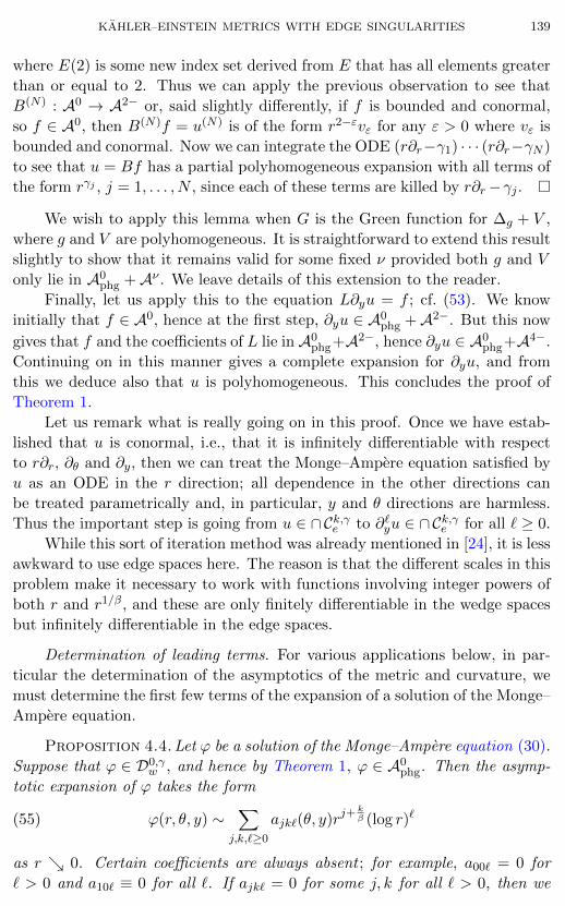
KAHLER–EINSTEIN METRICS WITH EDGE SINGULARITIES 139
where E(2) is some new index set derived from E that has all elements greater
than or equal to 2. Thus we can apply the previous observation to see that
B(N) : A0 → A2− or, said slightly differently, if f is bounded and conormal,
so f ∈ A0, then B(N)f = u(N) is of the form r2−εvε for any ε > 0 where vε is
bounded and conormal. Now we can integrate the ODE (r∂r−γ1) · · · (r∂r−γN )
to see that u = Bf has a partial polyhomogeneous expansion with all terms of
the form rγj , j = 1, . . . , N , since each of these terms are killed by r∂r−γj .
We wish to apply this lemma when G is the Green function for ∆g + V ,
where g and V are polyhomogeneous. It is straightforward to extend this result
slightly to show that it remains valid for some fixed ν provided both g and V
only lie in A0phg +Aν . We leave details of this extension to the reader.
Finally, let us apply this to the equation L∂yu = f ; cf. (53). We know
initially that f ∈ A0, hence at the first step, ∂yu ∈ A0phg +A2−. But this now
gives that f and the coefficients of L lie in A0phg+A2−, hence ∂yu ∈ A0
phg+A4−.
Continuing on in this manner gives a complete expansion for ∂yu, and from
this we deduce also that u is polyhomogeneous. This concludes the proof of
Theorem 1.
Let us remark what is really going on in this proof. Once we have estab-
lished that u is conormal, i.e., that it is infinitely differentiable with respect
to r∂r, ∂θ and ∂y, then we can treat the Monge–Ampere equation satisfied by
u as an ODE in the r direction; all dependence in the other directions can
be treated parametrically and, in particular, y and θ directions are harmless.
Thus the important step is going from u ∈ ∩Ck,γe to ∂`yu ∈ ∩Ck,γe for all ` ≥ 0.
While this sort of iteration method was already mentioned in [24], it is less
awkward to use edge spaces here. The reason is that the different scales in this
problem make it necessary to work with functions involving integer powers of
both r and r1/β, and these are only finitely differentiable in the wedge spaces
but infinitely differentiable in the edge spaces.
Determination of leading terms. For various applications below, in par-
ticular the determination of the asymptotics of the metric and curvature, we
must determine the first few terms of the expansion of a solution of the Monge–
Ampere equation.
Proposition 4.4. Let ϕ be a solution of the Monge–Ampere equation (30).
Suppose that ϕ ∈ D0,γw , and hence by Theorem 1, ϕ ∈ A0
phg. Then the asymp-
totic expansion of ϕ takes the form
(55) ϕ(r, θ, y) ∼∑
j,k,`≥0
ajk`(θ, y)rj+ k
β (log r)`
as r 0. Certain coefficients are always absent ; for example, a00` = 0 for
` > 0 and a10` ≡ 0 for all `. If ajk` = 0 for some j, k for all ` > 0, then we
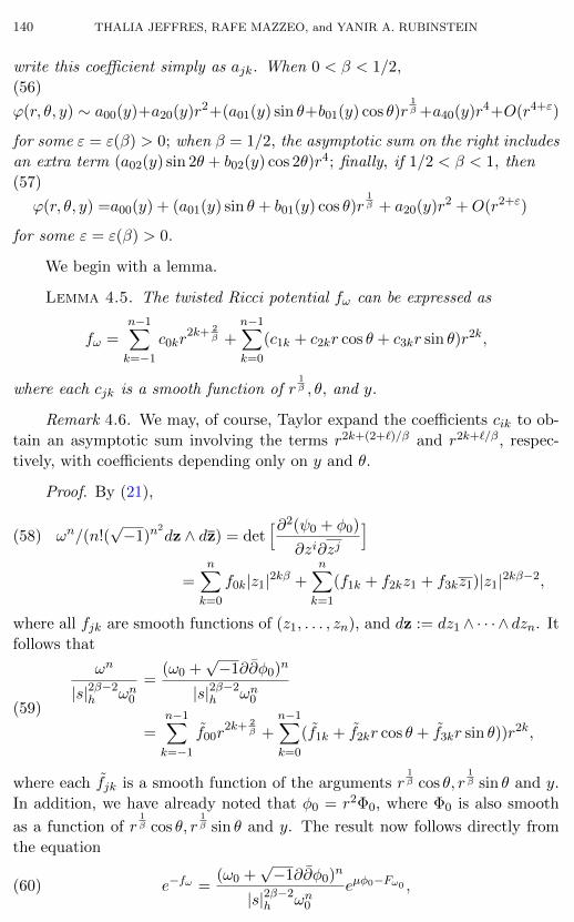
140 THALIA JEFFRES, RAFE MAZZEO, and YANIR A. RUBINSTEIN
write this coefficient simply as ajk. When 0 < β < 1/2,
(56)
ϕ(r, θ, y) ∼ a00(y)+a20(y)r2+(a01(y) sin θ+b01(y) cos θ)r1β +a40(y)r4+O(r4+ε)
for some ε = ε(β) > 0; when β = 1/2, the asymptotic sum on the right includes
an extra term (a02(y) sin 2θ + b02(y) cos 2θ)r4; finally, if 1/2 < β < 1, then
(57)
ϕ(r, θ, y) =a00(y) + (a01(y) sin θ + b01(y) cos θ)r1β + a20(y)r2 +O(r2+ε)
for some ε = ε(β) > 0.
We begin with a lemma.
Lemma 4.5. The twisted Ricci potential fω can be expressed as
fω =n−1∑k=−1
c0kr2k+ 2
β +n−1∑k=0
(c1k + c2kr cos θ + c3kr sin θ)r2k,
where each cjk is a smooth function of r1β , θ, and y.
Remark 4.6. We may, of course, Taylor expand the coefficients cik to ob-
tain an asymptotic sum involving the terms r2k+(2+`)/β and r2k+`/β, respec-
tively, with coefficients depending only on y and θ.
Proof. By (21),
(58) ωn/(n!(√−1)n
2dz ∧ dz) = det
[∂2(ψ0 + φ0)
∂zi∂zj
]=
n∑k=0
f0k|z1|2kβ +n∑k=1
(f1k + f2kz1 + f3kz1)|z1|2kβ−2,
where all fjk are smooth functions of (z1, . . . , zn), and dz := dz1 ∧ · · · ∧ dzn. It
follows that
(59)
ωn
|s|2β−2h ωn0
=(ω0 +
√−1∂∂φ0)n
|s|2β−2h ωn0
=n−1∑k=−1
f00r2k+ 2
β +n−1∑k=0
(f1k + f2kr cos θ + f3kr sin θ))r2k,
where each fjk is a smooth function of the arguments r1β cos θ, r
1β sin θ and y.
In addition, we have already noted that φ0 = r2Φ0, where Φ0 is also smooth
as a function of r1β cos θ, r
1β sin θ and y. The result now follows directly from
the equation
(60) e−fω =(ω0 +
√−1∂∂φ0)n
|s|2β−2h ωn0
eµφ0−Fω0 ,
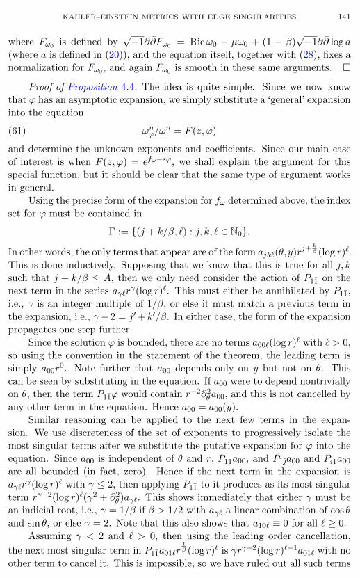
KAHLER–EINSTEIN METRICS WITH EDGE SINGULARITIES 141
where Fω0 is defined by√−1∂∂Fω0 = Ricω0 − µω0 + (1 − β)
√−1∂∂ log a
(where a is defined in (20)), and the equation itself, together with (28), fixes a
normalization for Fω0 , and again Fω0 is smooth in these same arguments.
Proof of Proposition 4.4. The idea is quite simple. Since we now know
that ϕ has an asymptotic expansion, we simply substitute a ‘general’ expansion
into the equation
(61) ωnϕ/ωn = F (z, ϕ)
and determine the unknown exponents and coefficients. Since our main case
of interest is when F (z, ϕ) = efω−sϕ, we shall explain the argument for this
special function, but it should be clear that the same type of argument works
in general.
Using the precise form of the expansion for fω determined above, the index
set for ϕ must be contained in
Γ := (j + k/β, `) : j, k, ` ∈ N0.
In other words, the only terms that appear are of the form ajk`(θ,y)rj+ k
β (log r)`.
This is done inductively. Supposing that we know that this is true for all j, k
such that j + k/β ≤ A, then we only need consider the action of P11 on the
next term in the series aγ`rγ(log r)`. This must either be annihilated by P11,
i.e., γ is an integer multiple of 1/β, or else it must match a previous term in
the expansion, i.e., γ− 2 = j′+ k′/β. In either case, the form of the expansion
propagates one step further.
Since the solution ϕ is bounded, there are no terms a00`(log r)` with ` > 0,
so using the convention in the statement of the theorem, the leading term is
simply a00r0. Note further that a00 depends only on y but not on θ. This
can be seen by substituting in the equation. If a00 were to depend nontrivially
on θ, then the term P11ϕ would contain r−2∂2θa00, and this is not cancelled by
any other term in the equation. Hence a00 = a00(y).
Similar reasoning can be applied to the next few terms in the expan-
sion. We use discreteness of the set of exponents to progressively isolate the
most singular terms after we substitute the putative expansion for ϕ into the
equation. Since a00 is independent of θ and r, P11a00, and P1a00 and Pi1a00
are all bounded (in fact, zero). Hence if the next term in the expansion is
aγ`rγ(log r)` with γ ≤ 2, then applying P11 to it produces as its most singular
term rγ−2(log r)`(γ2 + ∂2θ )aγ`. This shows immediately that either γ must be
an indicial root, i.e., γ = 1/β if β > 1/2 with aγ` a linear combination of cos θ
and sin θ, or else γ = 2. Note that this also shows that a10` ≡ 0 for all ` ≥ 0.
Assuming γ < 2 and ` > 0, then using the leading order cancellation,
the next most singular term in P11a01`r1β (log r)` is γrγ−2(log r)`−1a01` with no
other term to cancel it. This is impossible, so we have ruled out all such terms
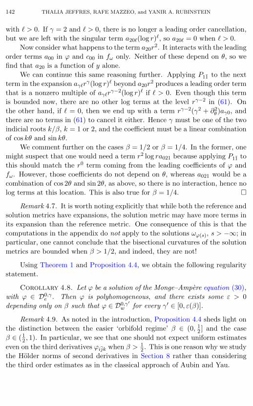
142 THALIA JEFFRES, RAFE MAZZEO, and YANIR A. RUBINSTEIN
with ` > 0. If γ = 2 and ` > 0, there is no longer a leading order cancellation,
but we are left with the singular term a20`(log r)`, so a20` = 0 when ` > 0.
Now consider what happens to the term a20r2. It interacts with the leading
order terms a00 in ϕ and c00 in fω only. Neither of these depend on θ, so we
find that a20 is a function of y alone.
We can continue this same reasoning further. Applying P11 to the next
term in the expansion aγ`rγ(log r)` beyond a20r
2 produces a leading order term
that is a nonzero multiple of aγ`rγ−2(log r)` if ` > 0. Even though this term
is bounded now, there are no other log terms at the level rγ−2 in (61). On
the other hand, if ` = 0, then we end up with a term rγ−2(γ2 + ∂2θ )aγ0, and
there are no terms in (61) to cancel it either. Hence γ must be one of the two
indicial roots k/β, k = 1 or 2, and the coefficient must be a linear combination
of cos kθ and sin kθ.
We comment further on the cases β = 1/2 or β = 1/4. In the former, one
might suspect that one would need a term r2 log ra021 because applying P11 to
this should match the r0 term coming from the leading coefficients of ϕ and
fω. However, those coefficients do not depend on θ, whereas a021 would be a
combination of cos 2θ and sin 2θ, as above, so there is no interaction, hence no
log terms at this location. This is also true for β = 1/4.
Remark 4.7. It is worth noting explicitly that while both the reference and
solution metrics have expansions, the solution metric may have more terms in
its expansion than the reference metric. One consequence of this is that the
computations in the appendix do not apply to the solutions ωϕ(s), s > −∞; in
particular, one cannot conclude that the bisectional curvatures of the solution
metrics are bounded when β > 1/2, and indeed, they are not!
Using Theorem 1 and Proposition 4.4, we obtain the following regularity
statement.
Corollary 4.8. Let ϕ be a solution of the Monge–Ampere equation (30),
with ϕ ∈ D0,γe . Then ϕ is polyhomogeneous, and there exists some ε > 0
depending only on β such that ϕ ∈ D0,γ′w for every γ′ ∈ [0, ε(β)].
Remark 4.9. As noted in the introduction, Proposition 4.4 sheds light on
the distinction between the easier ‘orbifold regime’ β ∈ (0, 12 ] and the case
β ∈ (12 , 1). In particular, we see that one should not expect uniform estimates
even on the third derivatives ϕijk when β > 12 . This is one reason why we study
the Holder norms of second derivatives in Section 8 rather than considering
the third order estimates as in the classical approach of Aubin and Yau.
KAHLER–EINSTEIN METRICS WITH EDGE SINGULARITIES 143
5. Maximum principle and the uniform estimate
We now recall the formulation of the maximum principle in this singular
setting. The main issue is to find barrier functions that allow one to reduce to
the classical maximum principle on M \D. These barrier functions were used
already in [33].
Lemma 5.1. Let f be continuous on M and satisfy |f(r, θ, y)−a(y)| ≤ Crγfor some a ∈ C0(D) and 0 < γ < 1. Then for ε sufficiently small,
(i) if C > 0, then f + C|s|εh achieves its maximum in M \D;
(ii) if c > 0 is small enough, then c|s|εh ∈ PSH(M,ω).
Proof. (i) The function |s|εh is comparable to rε/β, so for C > 0, r 7→f(r, θ, y)+C|s|εh strictly increases, hence it cannot reach its maximum at r = 0.
(ii) Let h be a smooth Hermitian metric on LD with global holomorphic
section s so that D = s−1(0). For any b ≥ 0, we have√−1∂∂b ≥ b
√−1∂∂ log b.
Setting b := |s|εh gives
(62)√−1∂∂b ≥
√−1 ε|s|εh∂∂ log |s|h = −1
2ε|s|εhR(h) > −Cω,
where C depends only on the choice of ω, h, s, ε. Thus C−1b ∈ PSH(M,ω).
The assumption on f above holds, in particular, for f ∈ C0,γw , and for f
and ∆ωf when f ∈ D0,γw .
This lemma is used as follows. Replacing |s|εh by c|s|εh and letting c tend
to 0, we obtain estimates that are the same as those one would expect from
the maximum principle on M\D. See the proofs of Lemmas 5.2 and 7.2 below
for more on this. The uniqueness and a priori C0 estimate when µ ≤ 0 are now
immediate consequences.
Lemma 5.2. Solutions to the Monge–Ampere equation (32) with s ≤ 0
are unique (when s = 0, only unique up to a constant) in D0,γw ∩ PSH(M,ω)
and satisfy
(63) ||ϕ(s, t)||C0(M) ≤ C = C(||fω||C0(M),M, ω).
Proof. Uniqueness when s < 0 is proved in [33]; that argument carries over
directly to this Monge–Ampere equation and either of the types of function
spaces we are using here, because of Lemma 5.1. Finally, when s = 0, the
result of B locki [14] gives uniqueness in L∞(M) up to a constant, and that
constant can be chosen by requiring that supϕ(0, t) = lims→0− supϕ(s, t).
The same argument also shows that ||ϕ(s, t)||C0(M) ≤ −2s−1||fω||C0(M) for
each s < 0. One can then obtain a uniform estimate for all s ≤ 0 as follows.
First, by the above, we may assume that s > S, for some S < 0. With respect
144 THALIA JEFFRES, RAFE MAZZEO, and YANIR A. RUBINSTEIN
to the fixed smooth Kahler form ω0, (32) can be rewritten as
ωnϕ = ωn0F |s|2β−2h etfω+ct−sϕ,
where F ∈ C0(M). By the previous estimate, ||etfω+ct−sϕ||C0(M) ≤ C uni-
formly in s. It follows that ||F |s|2β−2h etfω+ct−sϕ||Lp(M,ωn0 ) ≤ Cp, for all p ∈
(1, 1/(1 − β)), with Cp independent of s ≤ 0. Assuming this, by Ko lodziej’s
estimate [34], oscϕ(s, t) ≤ C, with C > 0 independent of s, t, and since by
(32) ϕ(s, t) changes sign, then also |ϕ(s, t)| ≤ C.
6. The uniform estimate in the positive case
In contrast to the nonpositive curvature cases, when µ > 0, there are
well-known obstructions to the existence of an a priori C0 estimate along the
continuity path. In this section we review the standard theory due to Tian
and others [61], [62] along with the necessary modifications to adapt it to our
setting. For an alternative variational approach that can be applied to more
general classes of plurisubharmonic functions, we refer to [9].
6.1. Poincare and Sobolev inequalities. In this subsection we show that
along the continuity path (30) one has uniform Poincare and Sobolev inequal-
ities.
We first prove that a uniform Poincare inequality holds as soon as s>ε>0.
The following argument is the analogue of [62, Lemma 6.12] in this edge setting
and also generalizes [41, Lemma 3] to higher dimensions. The second part is
the same assertion as [24, Prop. 8]. The proof here takes advantage of the fine
regularity results for solutions available to us.
Lemma 6.1. Denote by ∆ωϕ(s)the Friedrichs extension of the Laplacian
associated to ωϕ(s).
(i) For any s ∈ (0, µ), λ1(−∆ωϕ(s)) > s.
(ii) For s = µ, λ1(−∆ωϕ(µ)) ≥ µ. If (∆ωϕ(µ)
+ µ)ψ = 0, then ∇1,0gϕ(µ)
ψ is a
holomorphic vector field tangent to D.
Proof. (i) Let ψ be an eigenfunction of ∆ωϕ(s)with eigenvalue −λ1. Since
ϕ(s) is polyhomogeneous, then the eigenfunctions of ∆ωϕ(s)are also polyho-
mogeneous. This is a special case of the main regularity theorem for linear
elliptic differential edge operators from [43]. The proof uses the same pseu-
dodifferential machinery described in Section 3 (although for this particular
result, it is possible to give a more elementary proof). The key fact is that
ψ ∼ a0r0 + a1r
1β + a2r
2 + O(r2+η) for some η > 0 and, in particular, there is
no log r in this expansion, since we are using the Friedrichs extension.
KAHLER–EINSTEIN METRICS WITH EDGE SINGULARITIES 145
The Bochner–Weitzenbock formula states that on M \D,
1
2∆g|∇gf |2g = Ric (∇gf,∇gf) + |∇2f |2g +∇f · ∇(∆gf).
Since ∆g = 2∆ω and |∇2f |2g = 2|∇1,0∇1,0f |2 + 2(∆ωf)2, this becomes
(64) ∆ω|∇1,0ψ|2g = 2Ric (∇1,0ψ,∇0,1ψ)+2|∇1,0∇1,0ψ|2+2λ21ψ
2−4λ1|∇1,0ψ|2ω.
We now claim that
(65)
∫M
∆ωϕ |∇1,0ψ|2ωϕωnϕ = 0.
This follows directly from the expansion of ψ, since the worst term in the ex-
pansion of ∇1,0ψ is r1β−1
. Hence if we integrate over r ≥ ε, then the boundary
term is of order ε2β−2
(taking into account the measure rdθdy on this bound-
ary), and this tends to 0 with ε. This proves the claim. Thus integrating (64)
and using that Ricω(s) > sω(s) when s < µ, we see that λ1 > s.
(ii) When s = µ, this same argument yields λ1 ≥ µ. Moreover, equality
holds precisely when ∇1,0∇1,0ψ = 0 on M \ D; i.e., ∇1,0ψ is a holomorphic
vector field on M \D. Using the asymptotic expansion, ∇1,0ψ is continuous
up to D and hence extends holomorphically to M . Now, the coefficient of ∂∂ζ
equals g1ψ. By (13) g1 = O(rη′) and hence vanishes on D for j 6= 1 (and ψ is
infinitely differentiable in the j 6= 1 directions), while although g11 is uniformly
positive, ψ1 = O(r1β−1
), so this terms also vanishes on D. In conclusion, the∂∂ζ component of ∇1,0ψ vanishes at D, so this vector field is tangent to D.
We now estimate the Sobolev constant. First observe that the Sobolev
inequality holds for the model edge metric gβ, i.e., since dimM = 2n,
(66) ||f ||L
2nn−1 (M,gβ)
≤ CS ||f ||W 1,2(M,gβ),
and hence also for any metric uniformly equivalent to it. One way to prove this
is to note that it suffices to prove this inequality locally, in the neighbourhood
of any point; away from D this is just the standard Sobolev inequality, while in
a neighbourhood of any point p ∈ D we can use the (ζ, Z) coordinate system
to reduce to the standard Euclidean case. An alternate proof relies on the
well-known equivalence of the Sobolev inequality with the fact that the heat
kernel for the scalar Laplacian blows up like t−n as t 0 (since the overall
dimension is 2n). Since gβ is a product of a cone with a Euclidean space, this,
in turn, reduces to the fact that the heat kernel on a two-dimensional cone
blows up like t−1, which can be verified by direct computation; see, e.g., [24].
As an aside, observe that using (66), the standard Moser iteration proof
of the C0 estimate for s = 0 [62] goes through exactly as in the smooth case
and hence can be used instead of Ko lodziej’s estimate to prove Lemma 5.2.
146 THALIA JEFFRES, RAFE MAZZEO, and YANIR A. RUBINSTEIN
Next, we derive a uniform Sobolev inequality when s > ε. Our approach
follows Bakry [4] closely and relies on the general theory of diffusive semigroups.
The following result is essentially a special case of [4, Th. 6.10].
Proposition 6.2. Let ε ∈ (0, 1) and s ∈ (ε, 1]. There exists a uniform
constant C > 0, depending only on (M,ω), n and ε, so that for any f ∈W 1,2(M,ωϕ(s)),
||f ||L
2nn−1 (M,ωϕ(s))
≤ C||f ||W 1,2(M,ωϕ(s)).
Proof. Let L = ∆ωϕ . Proposition 2.1 in [4] (which holds for substantially
more general operators L) asserts that if A ⊂ DFr(L) (recall (40)) is a subspace
preserved by L and etL and dense in L2, then it is also dense in DFr(L) with
respect to the graph norm ||f ||L2 + ||Lf ||L2 . We can also verify this directly
in our setting and, in fact, have already done so in the proof of Lemma 4.2
above; but cf. also the discussion in [4, p. 35].
Now, for any two functions f, g ∈ A, define the quantities
(67) 2Γ(f, g) := L(fg)− fLg − gLf
and
(68) 2Γ2(f, g) := LΓ(f, g)− Γ(f, Lg)− Γ(g, Lf).
Note that on the smooth part M \D,
(69) Γ(f, f) = |∇f |2
(the gradient and norm are taken with respect to ωϕ) and
(70) Γ2(f, f) =1
2L|∇f |2 −∇f.∇Lf = Ricωϕ(∇f,∇f) + |∇2f |2.
Since f ∈ A, (69) holds on all of M as a W 1,2 distribution. Furthermore, by
virtue of (31), (70) implies that
(71) Γ2(f, f) ≥ CεΓ(f, f) +1
2n(Lf)2
in the sense of distributions on all of M , where C = C(n) is a universal
constant. Both of these assertions can be checked easily using that f is poly-
homogeneous with an expansion f = a0(y) + r1β (a1(y) cos θ + a2(y) sin θ) +
a2(y)r2 +O(r2+c) for some c > 0.
Following the definition and notation of [4, p. 93], we have proved that
L satisfies the “uniform curvature-dimension condition” CD(Cε, 2n). We can
then follow the general argument in [4] to obtain uniform Sobolev bounds [4,
Th. 6.10]; cf. also [5, Th. 1]. This procedure also leads to a uniform Poincare
estimate; however, an examination of the proof of [4, Prop. 6.3] shows that this
KAHLER–EINSTEIN METRICS WITH EDGE SINGULARITIES 147
is essentially equivalent to the one given above in Lemma 6.1(i). In any case,
we now sketch Bakry’s reasoning and explain in detail why it applies here.
The first point is that it suffices to prove the uniform Sobolev inequality
only for functions in A. Indeed, using the density of A in the graph norm,
we must show that both sides in the Sobolev inequality are continuous in
this topology. For the right-hand side, this is obvious. Since there is some
(not necessarily uniform) Sobolev inequality, cf. the paragraph containing (66),
W 1,2 is contained in L2nn−1 and so a sequence converging in W 1,2 converges
weakly in L2nn−1 , and so the left-hand side is also continuous in the appropriate
sense.
We now show uniform control of the Sobolev constant. Fix 2 < p < 2nn−1
and δ > 0, and let f(p)k ∈ A be a sequence which converges towards the
supremum of the ratio
(72)||F ||2p − (1 + δ)||F ||22
Γ(F, F )
over F ∈ DFr(L). Denote this supremum by γp. As usual, we can assume that
f(p)k ≥ 0 and ||f (p)
k ||2 = 1. Using the compactness of W 1,2 in Lp (which is a
consequence of the existence of a Sobolev inequality; for a general semigroup,
this compactness is not automatic and is proved in [4, Th. 4.11]), we can
extract a subsequence converging weakly in DFr(L) and strongly in Lp to a
nontrivial limit function f (p) ≥ 0, which we call f for simplicity. This satisfies
||f ||2p = (1 + δ) + γpΓ(f, f). Assuming that we have normalized the measure
associated to ωnϕ(s) to have unit volume, then f must be nonconstant since
δ > 0. Since f maximizes (72), the usual argument in the calculus of variations
gives ||f ||2−pp 〈fp−1, g〉 = (1 + δ)〈f, g〉 + γpΓ(f, g) = 〈f, (1 + δ)g − γpLg〉, for
any g ∈ DFr(L) or, equivalently, ||f ||2−pp 〈fp−1, Rλ(h)〉 = 〈f, γph〉. Here λ :=
(1 + δ)/γp and g = Rλ(h) where Rλ =∫∞0 e−λtetLdt = (λI − L)−1 is the
resolvent of L. This shows that f = Rλ(||f ||2−pp fp−1)/γp, or equivalently
(73) ||f ||2−pp fp−1 = ((1 + δ)− γpL)f.
Following [1, §3.2], the solution to this subcritical Yamabe-type equation must
be polyhomogeneous. Then, by a determination of the leading terms in the
expansion of f , it readily follows that f ∈ D0,γw . Both these assertions are
simpler analogues of Theorem 1 and Proposition 4.4, and their proof follows
similar, but simpler, arguments since this is a quasilinear equation and not a
fully nonlinear one. Thus, f ∈ A.
148 THALIA JEFFRES, RAFE MAZZEO, and YANIR A. RUBINSTEIN
Lemma 6.3. The constant γp associated to the embedding W 1,2 ⊂ Lp
satisfies
(74) γp ≤(2n− 1)(p− 2)(1 + δ)
2nCε.
Proof. Fix a ∈ R. We let g be such that ga = f ≡ f (p). We then divide
(73) by f and then substitute f = ga to get
(75)||f ||2−pp ga(p−2) = 1 + δ − γpg−a[aga−1Lg + a(a− 1)ga−2Γ(g, g)]
= 1 + δ − aγp[g−1Lg + (a− 1)g−2Γ(g, g)],
Now, following Bakry, we multiply this by −gLg and integrate:
−||f ||2−pp
¨g1+a(p−2), Lg
∂= (1 + δ)Γ(g, g) + aγp||Lg||2 + aγp(a− 1)
≠Lg
g,Γ(g, g)
∑.
The left-hand side can be rewritten as
||f ||2−pp Γ(g1+a(p−2), g) = Cp(1 + a(p− 2))〈ga(p−2),Γ(g, g)〉.
This can be rewritten using (75) as
(1 + a(p− 2))〈1 + δ − aγp[g−1Lg + (a− 1)g−2Γ(g, g)],Γ(g, g)〉.
Altogether, we have
(1 + a(p− 2))¨1 + δ − aγp[g−1Lg + (a− 1)g−2Γ(g, g)],Γ(g, g)
∂= (1 + δ)Γ(g, g) + aγp||Lg||2 + aγp(a− 1)
≠Lg
g,Γ(g, g)
∑.
So the constant ||f ||2−pp disappears; from this point on we follow Bakry, and
as in [4, (6.37)], we obtain
1 + δ
γp(p− 2)||Γ(g, g)||1
= ||Lg||22 + a(p− 1)〈Lg/g,Γ(g, g)〉+ (a− 1)(1 + a(p− 2))||Γ(g, g)/g||22.
We now invoke a consequence of (71), which holds by the chain rule [4, (6.38)]:
for any b ∈ R,
Γ2(g, g) + bΓ(g,Γ(g, g))/g+ b2(Γ(g, g)/g)2 ≥ CεΓ(g, g) +1
2n(Lg+ bΓ(g, g)/g)2.
Integrating givesÇ1 + δ
γp(p− 2)− 2n
2n− 1Cε
åΓ(g, g)
≥ ((a− 1)(1 + a(p− 2))− b(b+ 2n/(2n+ 1))) ||Γ(g, g)/g||22.
Choosing a, b appropriately as in [4, p. 110], we see that the right-hand side is
nonnegative, which implies a uniform bound on γp since Γ(g, g) ≥ 0.
KAHLER–EINSTEIN METRICS WITH EDGE SINGULARITIES 149
Letting p 2n/(n − 1), and using the fact that there is a Sobolev in-
equality at the critical exponent, we see that this Sobolev constant has the
upper bound (74) with p = 2n/(n − 1). This concludes the proof of Proposi-
tion 6.2.
Remark 6.4. In fact, [5, Th. 3] shows that we can find a uniform bound
for the diameter of (M,ωϕ(s)) from Proposition 6.2. Indeed, define
D(Γ) := sup|f(x)− f(y)| : x, y ∈M,f ∈ A, ||Γ(f, f)||L∞(M) ≤ 1,
and apply the Sobolev inequality to the functions (1 + λf)1−n2 for any f ∈ A.
(One must check that such functions are once again in A.) It then follows that
D(Γ) ≤ Cε−1/2.
Remark 6.5. There are other possible approaches to the estimation of the
Sobolev constants. One approach, suggested in a remark in the first version of
this article, is to approximate ωϕ(s) by smooth Kahler metrics with a uniform
positive lower bound on the Ricci curvature. This has been carried out in detail
in [63], [18]. Another approach is to show that as a metric-measure space,
the completion of (M \D,ωϕ, ωϕn) satisfies a uniform (generalized) doubling
property. The arguments of [30], [32] show that the Poincare inequality implies
a Sobolev inequality. This was described in detail in an earlier version of this
paper, but for brevity we have replaced this by the semigroup approach above.
6.2. Energy functionals. Unlike in the previous cases, there are well-known
obstructions to obtaining a C0 estimate in the positive case. The existence of
such an estimate is then described in terms of the behavior of certain energy
functionals. For more background, we refer to [3], [7], [56], [62].
The energy functionals I, J , introduced by Aubin [3], are defined by
I(ω, ωϕ) =1
V
∫M
√−1∂ϕ ∧ ∂ϕ ∧
n−1∑l=0
ωn−1−l ∧ ωϕl =1
V
∫Mϕ(ωn − ωnϕ),
J(ω, ωϕ) =V −1
n+ 1
∫M
√−1∂ϕ ∧ ∂ϕ ∧
n−1∑l=0
(n− l)ωn−l−1 ∧ ωϕl.
This definition certainly makes sense for pairs of smooth Kahler forms, and by
the continuity of the mixed Monge–Ampere operators on PSH(M,ω0)∩C0(M)
[8, Prop. 2.3], these functionals can be uniquely extended to pairs (ω0, ωϕ),
with ω0 smooth and ωϕ ∈ Hω0 , and hence also to Hω ×Hω, where now by ω
we mean the reference metric given by (26). These functionals are nonnegative
and equivalent:
(76)1
nJ ≤ I − J ≤ n
n+ 1I ≤ nJ.
One use of these functionals is in deriving a conditional C0 estimate.
150 THALIA JEFFRES, RAFE MAZZEO, and YANIR A. RUBINSTEIN
Lemma 6.6. Let s ∈ (0, µ). Any C0(M)∩PSH(M,ω) solution ϕ(s) to (30)
is unique. Moreover, if ϕ(s) ∈ D0,γs , then ||ϕ(s)||C0(M) ≤ C(1 + I(ω, ωϕ(s))) for
all s ∈ (ε, µ).
Proof. The uniqueness is due to Berndtsson [12]. We now prove the es-
timate. Using the uniform estimates on the Poincare and Sobolev constants,
the arguments proceed much as in the smooth case [62, Lemma 6.19].
First, let Gω be the Green function of −∆ω; i.e., −∆ωGω = −Gω∆ω =
Id − Π, where Π is the orthogonal projector onto the constants. (Note that
this is contrary to our previous sign convention for G, but it conforms with
the usual convention for this estimate.) Necessarily,∫M Gω(·, z)ωn(z) = 0. We
claim that Aω := − infM×M Gω < ∞. Assuming this for the moment, we can
write
ϕs(z) = V −1∫Mϕsω
n −∫MGω(x, y)∆ωϕs(y)ωn(y).
Hence, since −n < ∆ωϕs,
(77) supϕ(s) ≤ 1
V
∫Mϕ(s)ωn + nVAω.
To prove this claim about the Green function, recall that
G(z, z) =
∫ ∞0
(H(t, z, z)−Π(z, z)) dt,
where H is the heat kernel associated to this (Friedrichs) Laplacian and Π(z, z)
is the Schwartz kernel of this rank one projector. This integral converges
absolutely for any z 6= z. We rewrite this as
(78) G(z, z) =
∫ 1
0H(t, z, z) dt−Π(z, z) +
∫ ∞1
(H(t, z, z)−Π(z, z)) dt.
It follows easily from standard estimates that the integral from 1 to ∞ con-
verges to a bounded function. On the other hand, by the maximum principle,
H > 0, so the first term on the right is nonpositive. Finally, Π(z, z) = V −1 is
just a constant, so G is bounded below.
To conclude the proof, it suffices to prove − inf ϕ(s) ≤ −CV
∫M ϕ(s)ωnϕ(s).
(Indeed, ϕ(s) changes sign by the normalization (27) of fω, so ||ϕ(s)||C0(M) ≤oscϕ(s).) This can be shown in one of two ways. The first is by noting
that Bando–Mabuchi’s Green’s function lower bound [7] extends to our present
setting, and thus Aω(s) < C uniformly in s and − inf ϕ(s) ≤ − 1V
∫M ϕ(s)ωnϕ(s)+
nV C. Indeed, the proof of their bound relies on an estimate of Cheng–Li [20]
of the heat kernel Hω(s)(t, z, z)−V −1 ≤ Ct−n with C depending only on terms
of the Poincare and Sobolev constants, and hence independent of s > ε. Thus,
by (78) Aω(s) < C, as desired. The second uses Moser iteration, as in [56].
KAHLER–EINSTEIN METRICS WITH EDGE SINGULARITIES 151
6.3. Mabuchi ’s K-energy and Tian’s invariants. Define the twisted Mabuchi
K-energy functional by integration over paths ωϕt ⊂ Hω0 smooth in t,
(79) Eβ0 (ω, ωϕ) := − 1
V
∫M×[0,1]
ϕt∆ϕtfϕtωnϕt ∧ dt.
Its critical points are Kahler–Einstein edge metrics. The following is an exten-
sion of a formula of Tian [59, p. 254], [60, (5.12)] (cf. [9], [38]) to the twisted
setting. In particular it shows that Eβ0 is well defined on Hω0×Hω0 . The proof,
as others in this subsection, are straightforward extensions of their counter-
parts from the smooth setting and are included for the reader’s convenience.
Lemma 6.7. One has
(80) Eβ0 (ω, ωϕ) =1
V
∫M
logωnϕωnωnϕ − µ(I − J)(ω, ωϕ) +
1
V
∫Mfω(ωn − ωnϕ).
Proof. For any smooth (in t) path ωϕt ⊂ Hω connecting ω and ωϕ [62,
p. 70],
(81) (I − J)(ω, ωϕ1) = − 1
V
∫M×[0,1]
ϕt∆ϕtϕtωϕt ∧ dt.
Hence the variation of the right-hand side of (80) equals∫M
∆ϕϕ
Çlog
ωnϕωn
+ 1 + µϕ− fωåωnϕ,
and this coincides with dEβ0 (ϕ) since fωϕ = fω − µϕ − logωnϕωn + cϕ with cϕ a
constant. The formula then follows since both sides vanish when ωϕ = ω.
As noted in the introduction, a key property of the continuity path (30) is
the monotonicity of Eβ0 . Monotonicity of similar twisted K-energy functionals
was noted, e.g., in [52], and the following is the analogue of [52, Lemma 9.3].
Lemma 6.8. Eβ0 is monotonically decreasing along the continuity path
(30).
Proof. By (31),√−1∂∂fωϕ = −(µ − s)
√−1∂∂ϕ, and from (30), we have
(∆ϕ + s)ϕ = −ϕ. It follows that
d
dsEβ0 (ω, ωϕ(s)) = −µ− s
V
∫Mϕ∆ϕ(∆ϕ + s)ϕωnϕ,
and this is nonpositive by the positivity of ∆2ϕ + s∆ϕ, which is immediate for
s ≤ 0, and follows from Lemma 6.1, when s ∈ (0, µ).
Following Tian [61], we say that Eβ0 is proper if limj→∞(I−J)(ω, ωj) =∞implies that necessarily, limj→∞E
β0 (ω, ωj) = ∞. From Lemmas 6.6 and 6.8,
we have
152 THALIA JEFFRES, RAFE MAZZEO, and YANIR A. RUBINSTEIN
Corollary 6.9. Let ϕ(s) ∈ D0,γs ∩ PSH(M,ω). If Eβ0 is proper, then
||ϕ(s)||C0(M) ≤ C , independently of s ∈ (ε, µ).
We also note that, as observed by Berman [9], an alternative proof of
Corollary 6.9 follows by combining Ko lodziej’s estimate [34] and the following
result contained in [11, Lemma 6.4] and [9]. (Note that ϕ(s) change sign.)
Lemma 6.10 ([11], [9]). Suppose J(ω, ωϕ) ≤ C . Then for each t > 0,
there exists C ′ = C ′(C,M,ω, t) such that∫M e−t(ϕ−supϕ)ωn ≤ C ′.
We next recall the definition of Tian’s invariants [56], [58]:
αΩ,χ := supa : sup
ϕ∈PSH∩C∞(M,ω0)
∫Me−a(ϕ−supϕ)χn <∞
,
α(M) := αc1(M),ω0,
βΩ,ω := sup b : Ricχ ≥ bχ for some χ ∈ Hω,β(M) := sup b : Ricλ ≥ bλ for some λ ∈ H∞c1 ,
where the measure χn is assumed to have density in Lp(M,ωn0 ), for some p > 1,
and where, for emphasis, Hω is given by (18) and, when M is Fano, H∞c1 denotes
the space of smooth Kahler forms representing c1(M) (and finally, as always,
Ω = 1µc1(M) − 1−β
µ c1(LD) with Ω = [ω0] = [ω], ω0 a smooth Kahler form,
and ω = ω(β) the reference Kahler edge current). These invariants are always
positive as shown by Tian when χn is smooth, and hence also in general by
the Holder inequality. For some relations between αΩ,ω and αΩ,ω0 , we refer to
[9] where such invariants for singular measures were studied in depth.
Lemma 6.11. Suppose that αΩ,ω − nµn+1 > ε. Then Eβ0 ≥ εI −C for some
C ≥ 0.
Proof. Again we follow the classical argument [60, p. 164], [62, p. 95]. Note
that for any a ∈ (0, αω), there exists a constant Ca such that 1V
∫M log
ωnϕωnω
nϕ ≥
aI(ω, ωϕ)− Ca. Indeed, by (77) and Jensen’s inequality,
eCa ≥ 1
V
∫Me−a(ϕ− 1
V
∫Mϕωn)ωn
=1
V
∫Me− log
ωnϕωn−a(ϕ− 1
V
∫Mϕωn)ωnϕ ≥ e
− 1V
∫M
(logωnϕωn
+a(ϕ− 1V
∫Mϕωn))ωnϕ .
By (76) and (80) it then follows that Eβ0 ≥ (a− nµn+1)I − C.
Corollary 6.12. For all s ∈ (−∞, n+1n αΩ,ω) ∩ (−∞, µ], we have
||ϕ(s)||C0(M) ≤ C,
with C independent of s.
KAHLER–EINSTEIN METRICS WITH EDGE SINGULARITIES 153
Proof. When αΩ,ω >nµn+1 , the result follows from Lemma 6.11 and Corol-
lary 6.9. (Note, as explained in Section 9, that there is no difficulty in treating
the interval s ∈ (0, ε) for some ε > 0.) In general, the classical derivation [62]
carries over.
This conditional C0 estimate implies of course, given the other ingredients
of the proof of Theorem 2, that βΩ,ω ≥ minµ, n+1n αΩ,ω, just as in the smooth
setting. We remark that Donaldson [23] conjectured that when D ⊂ M is a
smooth anticanonical divisor of a Fano manifold, then β(M) = supβ : (29)
admits a solution with µ = β . Note that the Calabi–Yau theorem shows that
the left-hand side is positive, while Corollary 1 shows that the right-hand side
is positive. Our results have further direct bearings on this problem, which we
hope to discuss elsewhere.
7. The Laplacian estimate
Let f : M → N be a holomorphic map between two complex manifolds.
The Chern–Lu inequality was originally used by Lu to bound |∂f |2 when the
target manifold has negative bisectional curvature [40] under some technical
assumptions. This inequality was later used by Yau [69] together with his
maximum principle to greatly generalize the result to the case where (M,ω) is
a complete Kahler manifold with a lower bound C1 on the Ricci curvature, and
(N, η) is a Hermitian manifold whose bisectional curvature is bounded above
by a negative constant −C3. These results lead to Yau’s Schwarz lemma, which
says that the map f decreases distances in a manner depending only on C3 > 0
and C1.
In a related direction, the use of the Chern–Lu inequality to prove a
Laplacian estimate for complex Monge–Ampere equations seems to go back in
print at least to Bando–Kobayashi [6], who considered the case Ricω ≥ −C2η
and C3 arbitrary (not necessarily positive) in the context of constructing a
Ricci flat metric on the complement of a divisor. Next, the case Ricω ≥ −C1ω
(and again C3 arbitrary) was used in proving the a priori Laplacian estimate
for the Ricci iteration [52].
The point of Proposition 7.1 below is to state the Chern–Lu inequality
in a unified manner that applies to a wide range of Monge–Ampere equations
that appear naturally in Kahler geometry. It makes the Laplacian estimate
in these settings slightly simpler and the explicit dependence on the geometry
more transparent. In addition, the Chern–Lu inequality applies in some situa-
tions where the standard derivation [2], [70], [54] of the Aubin–Yau Laplacian
estimate may fail (as in the case of the Ricci iteration) or give an estimate with
different dependence on the geometry (which will be crucial in our setting).
While Proposition 7.1 below should be folklore among experts, it seems that
154 THALIA JEFFRES, RAFE MAZZEO, and YANIR A. RUBINSTEIN
it is less well known than it deserves to be. In particular, we are not aware of
a treatment of the Aubin–Yau or Calabi–Yau theorems that uses it.
7.1. The Chern–Lu inequality. Let (M,ω), (N, η) be compact Kahler man-
ifolds and let f : M → N be a holomorphic map with ∂f 6= 0. The Chern–Lu
inequality [21], [40] is
(82) ∆ω log |∂f |2 ≥ Ricω ⊗ η(∂f, ∂f)
|∂f |2− ω ⊗RN (∂f, ∂f, ∂f, ∂f)
|∂f |2on M.
Since the original statement [39, (7.13)], [40, (4.13)] contains a misprint, we
include a direct and slightly simplified derivation (since we restrict to the
Kahler setting) for completeness. We note also that (82) can be obtained as a
special case of a formula of Eells–Sampson [25, (16)] on the Laplacian of the
energy density of a harmonic map.
Write ∂f : T 1,0M → T 1,0N . Then ∂f is a section of T 1,0 ?M ⊗ T 1,0N
given in local holomorphic coordinates by ∂f = ∂f i
∂zjdzj ⊗ ∂
∂wi. With respect to
the metric induced by ω and η on the product bundle above,
(83) u := |∂f |2 = gilhjk∂f j
∂zi∂fk
∂zl.
Compute in normal coordinates at a point
∆ωu =∑p
upp = −∑i,l,p
gli,pphjkfj,if
k,l +
∑i,p
hjk,dmfd,pf
m,p f
ji f
k,i +
∑i,j,p
f j,ipf,ip
= Ricω ⊗ η(∂f, ∂f)− ω ⊗RN (∂f, ∂f, ∂f, ∂f) +∑i,j,p
f j,ipf,ip.
By the Cauchy–Schwarz inequality,
u∑i,j,p
f j,ipf,ip≥∑k
ukuk,
and since ∆ω log u = ∆ωu/u−∑k ukuk/u
2, the desired inequality follows.
One particularly useful form of the Chern–Lu inequality is when f is the
identity map.
Proposition 7.1. In the above, let f = id : (M,ω) → (M,η) be the
identity map, and assume that Ricω ≥ −C1ω − C2η and that Bisecη ≤ C3 for
some C1, C2, C3 ∈ R. Then,
(84) ∆ω log |∂f |2 ≥ −C1 − (C2 + 2C3)|∂f |2.
In particular, if ω = η +√−1∂∂ϕ, then
(85) ∆ω
Älog trωη − (C2 + 2C3 + 1)ϕ
ä≥ −C1 − (C2 + 2C3 + 1)n+ trωη.
Hence, ω ≥ Cη for some C > 0 depending only on C1, C2, C3, n and ||ϕ||C0(M).
KAHLER–EINSTEIN METRICS WITH EDGE SINGULARITIES 155
Proof. By (83), u = trωη. The assumption on Ricω implies that
Ricω ⊗ η(∂f, ∂f) = gilgkRihkl ≥ −C1gilgkgihkl − C2g
ilgkhihkl
= −C1trωη − C2(η, η)ω ≥ −C1trωη − C2(trωη)2,
where the last inequality follows from the identity [13, Lemma 2.77]
(η, η)ω = (trωη)2 − n(n− 1)η ∧ η ∧ ωn−2
ωn.
Similarly, we also have
−ω ⊗RN (∂f, ∂f, ∂f, ∂f) = −gigklRNikl≥ −C3g
igkl(hihkl + hilhk) ≥ −2C3(trωη)2.
Thus, (84) follows from (82). Since trωη = n − ∆ωϕ, equation (85) follows
from (84).
7.2. The Laplacian estimate in the singular Holder spaces. We now ap-
ply the Chern–Lu inequality to obtain an a priori Laplacian estimate for the
continuity method (32). For solutions of (30), it gives a bound depending, in
addition to the uniform norm, on an upper bound on the bisectional curvature
of the reference metric; in contrast, the well-known Aubin–Yau bound depends
on a lower bound for the bisectional curvature [2], [70], [54].
Lemma 7.2. Suppose that there exists a reference metric ω ∈ Hω0 with
Ricω ≥ −C2ω and Bisecω ≤ C3 on M \D, where C2 ∈ R ∪ ∞, C3 ∈ R. Let
s > S. Solutions to (32) in D0,γs ∩ C4(M \D) ∩ PSH(M,ω) satisfy
(86)||∆ωϕ(s, t)||C0(M) ≤ C = C(||fω||C0(M), ||ϕ(s, t)||C0(M), S, (1− t)C2, C3),
where (1−t)C2 is understood to be 0 when t = 1. Moreover, 1Cω ≤ ωϕ(s) ≤ Cω.
Proof. Along the continuity path (32),
Ricωϕ = (1− t)Ricω+ sωϕ + (µt− s)ω+ 2π(1− β)[D] ≥ Sωϕs,t − (1− t)C2ω.
Hence, the assumptions of Proposition 7.1 are satisfied (we take id : (M,ωϕ)→(M,ω)), and the desired estimates follow directly from (85) if the maximum
of (the bounded function) log trωϕω −Aϕ takes place in M \D.
Next, suppose the maximum is attained on D. We claim that log trωϕω ∈C0,γs for any γ ≤ min 1
β − 1, γ. Indeed, in the local coordinates z1, . . . , zn,
gijϕ = 1det gϕ
Aij , where A is the cofactor matrix of [gϕ]. Since Ai is a poly-
nomial in the components gϕk ¯, it too lies in C0,γs . In addition, 1/ det gϕ =
e−fω−ct+sϕ/det gω = |z1|2−2βF for some F ∈ C0,γs , hence this lies in C0,γ
s for
γ ≤ 1β − 1. Hence trωϕω = gijϕ gij ∈ C0,γ
s , proving the claim.
156 THALIA JEFFRES, RAFE MAZZEO, and YANIR A. RUBINSTEIN
Now by Lemma 5.1 applied to f := log trωϕω−Aϕ, we have that f + |s|εhachieves its maximum away from D for ε < βγ. (When s = e, we use that
ϕ ∈ Aphg by Theorem 1.) By (85) and Lemma 5.1(ii) (and in particular (62)),
for all sufficiently large N > 1, we have
∆ϕ(f +N−1|s|εh) ≥ −C1 − (2C3 + 1)n+ (1− C/N)trωϕω.
The maximum principle thus implies trωϕω ≤ C = C(C1, C3, ||ϕ||C0(M), ω),
and so ωϕ ≥ Cω. Going back to (30) we have ωnϕ ≤ Cωn (with C depending
on ||fω||C0(M) and ||ϕ(s, t)||C0(M)), and so also ωϕ ≤ Cω.
8. Holder estimates for second derivatives
In the interior of M \D, the Evans–Krylov regularity theory for Monge–
Ampere equations (Theorem 4.1) may be applied to obtain the a priori interior
C2,γ estimate for a solution ϕ on any ball B′ depending on C0 estimates for
ϕ and ∆ωϕ on a slightly larger ball. This depends heavily, of course, on the
uniform ellipticity of the Laplacian, and hence it does not apply directly for
balls arbitrarily close to D.
We now explain how to obtain a priori estimates in D0,γw using the a priori
Laplacian estimate from the last section. The proof uses an old argument due
to Tian.
Theorem 8.1. Let ϕ(s) ∈ D0,0w ∩ C4(M \ D) ∩ PSH(M,ω) be a solution
to (30) with s > S and 0 < β ≤ 1. Then
||ϕ(s)||D0,γw≤ C,
where C = C(S, β, ω, n, ||∆ωϕ||L∞(M), ||ϕ||L∞(M)).
Proof. Let U be a neighborhood in M . According to Theorem B.1, if ωϕ is
locally represented by uijdzi∧dzj on U \D, then for some fixed γ, r0 > 0, every
a ∈ (0, r0) and all x such that Ba(x) ⊂ U , we have ||∇uij ||2Ba(x) ≤ C a2n−2+2γ .
The constants γ, r0, C are all uniformly controlled. The Poincare inequality
gives ||uij−Cx,a||2Ba(x) ≤ C a2n+2γ , where Cx,a =∫Ba(x) uijω
n/∫Ba(x) ω
n. Using
the integral characterization of Holder spaces, see [31, Th. 3.1] for example,
patching up the estimates over a finite cover, and using that we already have
uniform bounds on ∆ωϕ itself, it follows that ||∆ωϕ||C0,γw≤ C.
The proof of Theorem B.1 requires the following lemma that is perhaps
of independent interest. Let ψ be a fixed Kahler potential for ω valid in a
neighborhood of y0 ∈ D. For each pair of parameters (s, t), consider the
function h = h(s, t) defined by the equality
(87) log h := logF + log det[ψij ] = tfω + ct − sϕ+ log det[ψij ].
By Lemma 2.2 (see (24)), ψ ∈ D0,γw for any γ ∈ (0, 1
β − 1].
KAHLER–EINSTEIN METRICS WITH EDGE SINGULARITIES 157
We now state a collection of estimates for h, but we note that only the
Lipschitz bound (iv) is used later in the proof of Theorem B.1.
Lemma 8.2. Define h = h(s, t) by (87), with s > S. Then the following
estimates hold with constants independent of t, s:
(i) For β ≤ 1, ||h(s, t)||C0(M) ≤ C(S,M,ω, β, ||ϕ(s, t)||C0(M)).
(ii) For β ≤ 1/2, ||h(s, t)||D0,0w≤ C = C(S,M,ω, β, ||∆ωϕ(s, t)||C0).
(iii) For β ≤ 2/3, ||h(s, t)||w;0,1 ≤ C = C(S,M,ω, β, ||ϕ(s, t)||C0,1w
).
(iv) For β ≤ 1,
(88) ||h(s, 1)||w;1, 1β−1 ≤ C = C(S,M,ω, β, ||ϕ(s, 1)||
C1, 1β−1
w
).
Moreover, ||h(s, 1)kl||C0(M) ≤ C(S,M,ω, β, ||∆ωϕ(s, 1)||C0).
Proof. By (58) and (8), near D,
det[ψi] = β2|ζ|2β−2
det[∂2(ψ0 + φ0)
∂zi∂zj
]= β2
n∑k=0
f0k|ζ|2k−2+ 2β + β2
n−1∑k=0
(f1k + f2kζ1β + f3kζ
1β )|ζ|2k,
with fjk smooth functions of (z1, . . . , zn). Thus, if β ∈ (0, 2/3], then log det[ψij ]
is in C0,1w . Moreover, if β ∈ (0, 1/2], then log det[ψij ] is in C1,1
w ; for that it suffices
to remark that
∂rfjk =∂fjk∂ρ
∂ρ
∂r=∂fjk∂ρ
(βr)1β−1 ∈ C0,1
w
if β ∈ (0, 1/2]. Next, by Lemma 4.5, and the same reasoning as above, it
follows that when β ∈ (0, 1/2], fω ∈ C1,1w and that when β ∈ (0, 2/3], fω ∈ C0,1
w .
Therefore, (ii) and (iii) follow. Note also that the above computations show
that fω,det[ψij ] ∈ L∞(M) for all β ∈ (0, 1], proving (i).
Now, assume t = 1. Denote, as before, dz = dz1 ∧ · · · ∧ dzn. By (60),
fω + log det[ψij ] = fω + log(ω0 +
√−1∂∂ψ0)n
(√−1)n2dζ ∧ dζ ∧ dz2 ∧ dz2 ∧ · · · ∧ dzn ∧ dzn
= fω + log(ω0 +
√−1∂∂ψ0)n
|z1|2β−2(√−1)n2dz ∧ dz
= log|s|2β−2
h ωn0 eFω0−µφ0
|z1|2β−2(√−1)n2dz ∧ dz
= (2β − 2) log a+ Fω0 − µφ0 + log det[ ∂2ψ0
∂zi∂zj
],
where a is defined in (20). Thus fω + log det[ψij ] can be written as a sum
Φ1−µφ0 = Φ1−µr2Φ0 with Φi, i = 0, 1, smooth functions of (z1, z1, . . . , zn, zn).
Hence, by the reasoning above, fω+log det[ψij ] ∈ C1, 1β−1
w , and therefore h(s, 1)
158 THALIA JEFFRES, RAFE MAZZEO, and YANIR A. RUBINSTEIN
belongs to C1, 1β−1
w as soon as ϕ(s, 1) does. The statement about the (1, 1)-part
of the Hessian of h(s, 1) follows in the same way. This concludes the proof
of (iv).
9. Existence of Kahler–Einstein edge metrics
We now conclude the proof of Theorem 2 on the existence of Kahler–
Einstein edge metrics, as well as of the convergence of the twisted Ricci itera-
tion (Theorem 2.5). We then describe the additional regularity properties as
stated in Theorem 2.
Starting the continuity path. Intuitively, the Ricci continuity path (30) has
the trivial solution ω(−∞) = ω at s = −∞. Even if one could make rigorous
sense of this, one could not apply the implicit function theorem directly to
obtain solutions for large negative finite values of s. Indeed, reparametrizing
(30) by setting σ = −1/s, then the linearization of the Monge-Ampere equation
at σ equals σ∆ϕ(−1/σ) − 1, and this degenerates at σ = 0. It is therefore
necessary to find a different way to produce a solution of (30) for sufficiently
negative, but finite, values of s. Once this has been accomplished, we can then
proceed with the rest of the continuity method.
When β ∈ (0, 1/2], this difficulty can be circumvented by using the two-
parameter family; see Remark 2.4. Indeed, as described in Section 2.4, the
original continuity path (30) embeds into the two-parameter family (32), and
it is trivial that solutions exist for the finite parameter values (s, 0). Unfor-
tunately, the a priori estimates needed to carry out the rest of the continuity
argument for the two-parameter family hold only when β ≤ 1/2. Thus, to
handle the general case, we must use another method to obtain a solution of
(30) for some large negative value of s. Wu [68, Prop. 7.3] used a Newton
iteration argument to obtain such a solution in a different setting. However,
his argument requires a lower Ricci curvature bound on the reference metric
(see [68, p. 431]), which we lack. In other words, no small multiple of fω be-
longs to Hω. What follows is an adaptation of Wu’s argument that requires
no curvature control on the reference metric.
Reformulate the original complex Monge–Ampere equation in terms of the
operator
Nσ : D0,γw → C0,γ
w , Nσ(Φ) := log(ωnσΦ/efωωn)− Φ.
As we remark at the end of this argument, the following argument works
equally well in the edge spaces and leads to the same conclusion. Observe that
DNσ|Φ = σ∆σΦ− Id. Now, suppose that σΦ ∈ Hω∩Aphg. By Proposition 3.2,
DNσ|Φ : D0,γw → C0,γ
w is Fredholm of index 0, and by the maximum principle
and Lemma 5.1, its nullspace K is trivial when s < 0. Hence, this operator is
KAHLER–EINSTEIN METRICS WITH EDGE SINGULARITIES 159
an isomorphism from D0,γw to C0,γ
w , with
(89) ||u||D0,γw≤ C||DNσu||C0,γ
w.
Denote by DNσ|−1Φ the inverse of this map on C0,γ
w .
We now set up the iteration method that will converge to a solution (New-
ton iteration for Nσ). Define a sequence of elements Φk ∈ D0,γe by setting
Φ0 = 0 and then
Φk = (Id−DNσ|−1Φk−1
Nσ)(Φk−1), k ∈ N
or, equivalently,
(90) Φk − Φk−1 −DNσ|−1Φk−1
Nσ(Φk−1) = 0.
When Φ ∈ A0phg, DNσ|−1
Φ preserves polyhomogeneity, so each of the successive
Φk are polyhomogeneous. Since Nσ(−fω) = 0 when σ = 0, it might seem more
natural to set Φ0 = −fω. However, this would cause a problem at the very
next step since, as already observed two paragraphs above,√−1∂∂fω blows
up at r = 0 when β > 1/2.
Next, observe that
(91)
Nσ(Φk) = Nσ(Φk)−Nσ(Φk−1)−DNσ|Φk−1(Φk − Φk−1)
=
∫ 1
0(1− c)D2Nσ|cΦk+(1−c)Φk−1
(Φk − Φk−1,Φk − Φk−1) dc.
This will be estimated using the equality D2Nσ|Φ(a, b) = σ2(∂∂a, ∂∂b)ωσΦ ,
which holds provided σΦ ∈ Hω. We now deduce inductively the sequences of
estimates
(92) ||Φj − Φj−1||D0,γw≤ C1||Nσ(Φj−1)||C0,γ
w
and
(93) ||Nσ(Φj)||C0,γw≤ C2σ
2||Φj − Φj−1||2D0,γw
for every j ≥ 1 with constants C1 and C2 independent of j. Suppose then that
these hold for every j ≤ k. We shall prove that they hold also for j = k + 1
with the same constants Ci.
First note that Φk = Φk − Φ0 =∑kj=1(Φj − Φj−1). Using (92) and (93)
iteratively gives
||Φj − Φj−1||D0,γw≤ C1C2σ
2||Φj−1 − Φj−2||2D0,γw≤ (C1C2σ
2)2j−1−1||Φ1||2j−1
D0,γw,
and then ||Nσ(Φj)||C0,γw≤ C2σ
2(C1C2σ2)2j−1−1||Φ1||2
j−1
D0,γw. We conclude that
||Φk||D0,γw≤
k∑j=1
||Φj − Φj−1||D0,γw≤ 2||Φ1||D0,γ
w,
160 THALIA JEFFRES, RAFE MAZZEO, and YANIR A. RUBINSTEIN
provided C1C2σ2||Φ1||D0,γ
w≤1/2. Thus if σ is sufficiently small, then ||σΦk||D0,γ
w
≤ η for some fixed η > 0. So, σΦk ∈ Hω, and if we let C1 denote the supremum
of the norm of DNσ|−1Φ among all Φ with ||Φ||D0,γ
w≤ η, then (92) holds with k
replaced by k + 1 and the same C1.
To obtain the final estimate, note that σ(cΦk + (1 − c)Φk−1) lies in the
same ball of radius η for 0 ≤ c ≤ 1, hence also in Hω, which means that (91)
with k replaced by k+ 1 can be estimated as before; C2 is the constant needed
to estimate this integral, which is uniform so long as cΦk + (1− c)Φk−1 remain
in the fixed η ball. This proves (93) with k replaced by k + 1.
We may now conclude that Φ∞ := limk→∞Φk =∑∞k=0(Φk+1 −Φk) exists
and lies in the same η ball in D0,γw , so σΦ∞ ∈ Hω.
Finally, by Theorem 1, Φ∞ is polyhomogeneous.
Openness. Define Ms,t : D0,γw → C0,γ
w by
Ms,t(ϕ) := logωnϕωn− tfω + sϕ, (s, t) ∈ A = (−∞, 0]× [0, 1] ∪ [0, µ]× 1.
Note that Ms,0(0) = 0. If ϕ(s, t) ∈ D0,γw ∩ PSH(M,ω) is a solution of (32), we
claim that its linearization
(94) DMs,t|ϕ(s,t) = ∆ϕ(s,t) + s : D0,γw → C0,γ
w , (s, t) ∈ A,
is an isomorphism when s 6= 0. If s = 0, this map is an isomorphism if we
restrict on each side to the codimension one subspace of functions with integral
equal to 0. Furthermore, we also claim that D0,γw × A 3 (ϕ, s, t) 7→ Ms,t(ϕ) ∈
C0,γw is a C1 mapping. Given these claims, the Implicit Function Theorem then
guarantees the existence of a solution ϕ(s, t) ∈ D0,γw for all (s, t) ∈ A sufficiently
close to (s, t).
Proposition 3.2 asserts that (94) is Fredholm of index 0 for any (s, t) ∈ A,
and by Proposition 3.3,
(95) ||u||D0,γw≤ C(||DMs,tu||C0,γ
w+ ||u||C0),
Its nullspace K is clearly trivial when s < 0, and also by Lemma 6.1 for (s, 1)
with s ∈ (0, µ); finally, when s = 0 it consists of constants. Thus DMs,t
is an isomorphism when s 6= 0 and is an isomorphism on the L2 orthogonal
complement to the constants when s = 0. This proves the first claim.
The second claim follows from (94) and Corollary 3.5, which shows that
the domains of these linearizations at different ϕ are all the same. The smooth
dependence on (s, t) is obvious.
Note finally that using (95), nearby solutions remain in PSH(M,ω).
We have written this out explicitly for the wedge spaces, but note that
all of these arguments go through verbatim for the edge spaces. Observe,
however, that using the results of Section 4, the nearby solutions are necessarily
polyhomogeneous.
KAHLER–EINSTEIN METRICS WITH EDGE SINGULARITIES 161
Closedness. Fix some S < 0, and denote AS := (s, t) ∈ A : s ∈ (S, 0].Let (sj , tj) be a sequence in intAS converging to (s, t) ∈ AS , and let
ϕ(sj , tj) ∈ D0,γw ∩ PSH(M,ω) be solutions to (32). Under the assumptions of
Theorem 2, the results of Sections 5, 7 and 8 imply that ||ϕ(sj , tj)||D0,γw≤ C,
where C depends on S, a lower bound on the Ricci curvature of ω times
(1−minj tj), and an upper bound on its bisectional curvature, both over M\D;
alternatively, the Aubin–Yau Laplacian estimate [2], [70], [54] gives a bound
depending on S and a lower bound on the bisectional curvature of ω over M\D.
Thus, when β ∈ (0, 12 ] ∪ 1, Lemma 2.3 implies that either type of bounds
give a uniform estimate ||ϕ(s, t)||D0,γw≤ C for all (s, t) ∈ AS . In general, re-
strict to the path (30) (i.e., let tj = 1 for all j) and then ||ϕ(s, 1)||D0,γw≤ C
for all s ∈ (S, 0] by Proposition A.1 and the results of Sections 5, 7 and 8.
Thus, for any γ′ ∈ (0, γ), there is a subsequence that converges in D0,γ′w such
that the limit function ϕ(s, 1) lies in D0,γw . Observe that Ms,1(ϕ(s, 1)) = 0 and
ϕ(s, 1) ∈ C∞(M \D).
Letting S → −∞, we obtain a solution for all (s, t) ∈ A∞ in the case
β ∈ (0, 12 ] ∪ 1 and for all (s, 1) ∈ (−∞, 0] × 1 in the general case. Now
by openness in A about the solution at (0, 1) (cf. [3], [7]), there exist so-
lutions also for [0, ε) × 1 ⊂ A. Then by Corollary 6.9 and the previous
arguments we obtain solutions for all (s, t) ∈ A when β ∈ (0, 12 ] ∪ 1 and for
all (s, 1) ∈ (−∞, µ] × 1 in the general case. By Theorem 1, these solutions
are polyhomogeneous. Finally, ϕ(s, t) ∈ PSH(M,ω). (This follows from a con-
tinuity argument, observing that the right-hand side of the Monge–Ampere
equation is positive.)
Regularity. Using the steps above, we obtain a solution ϕ := ϕ(µ, 1) ∈A0
phg ∩PSH(M,ω) to (30). Denote by gµ the associated Kahler–Einstein edge
metric. Using Proposition 4.4 and (6), gµ is asymptotically equivalent to the
reference metric g and, moreover, by the explicit form of the expansion and the
fact that P11 annihilates the r0 and r1β terms, we obtain that ϕ ∈ A0∩D0,ε(β)
w ,
where ε(β) is determined by Proposition 4.4 (see Corollary 4.8). This completes
the proof of Theorem 2.
Convergence of the Ricci iteration. We use the notation of Section 2.5.
As noted there, µ − 1τ plays the role of s. Consider first the case µ ≤ 0.
By the earlier analysis of (30), for any τ > 0, the iteration exists uniquely
and ψkτk∈N ⊂ D0,γw . By Lemma 5.1, the inductive maximum principle ar-
gument of [52] yields |ψkτ | ≤ C. Along the iteration, just as for the path
(30), the Ricci curvature is bounded from below by µ − 1τ , hence Proposi-
tion 7.1 and Lemma 5.1 show that |∆ωkτψkτ | ≤ C. (We consider the maps
id : (M,ωkτ ) → (M,ω).) Going back to equation (33) and using the C0 es-
timate then shows that |∆ωψkτ | ≤ C, hence by Theorem 8.1, |ψkτ |D0,γw≤ C.
162 APPENDIX BY CHI LI AND YANIR A. RUBINSTEIN
Thus a subsequence converges (as explained above for the continuity method)
to an element ψ∞ of D0,γw ∩C∞(M\D). Since each step in the iteration follows
a continuity path of the form (30) with ω replaced by ωkτ , Lemma 6.8 im-
plies that Eβ0 (ω(k−1)τ , ωkτ ) < 0 (unless ω was already Kahler–Einstein). Since
Eβ0 is an exact energy functional, i.e., satisfies a cocyle condition [42], then
Eβ0 (ω, ωkτ ) =∑kj=1E
β0 (ω(j−1)τ , ωjτ ) < 0. Therefore, ψ∞ is a fixed point of Eβ0 ,
hence a Kahler–Einstein edge metric. By Lemma 5.2 such Kahler–Einstein
metrics are unique; we conclude that the original iteration converges to ψ∞both in A0 and in D0,γ′
w for each γ′ ∈ (0, γ).
Next, consider the case µ > 0, and take µ = 1 for simplicity. By the
properness assumption, Corollary 6.9 implies the iteration exists (uniquely by
Lemma 6.6) for each τ ∈ (0,∞) and then the monotonicity of Eβ0 implies
that J(ω, ωkτ ) ≤ C. To obtain a uniform estimate on oscψkτ we will employ
the argument of [10] as explained to us by Berman. By Lemma 6.10, have∫M e−p(ψkτ−supψkτ )ωn ≤ C, where p/3 = max1− 1
τ ,1τ . Now rewrite (33) as
(96) ωnψkτ = ωnefω−(1− 1τ
)ψkτ− 1τψ(k−1)τ .
Using Ko lodziej’s estimate and the Holder inequality this yields the uniform
estimate oscψkτ ≤ C. Unlike for solutions of (30), the functions ψkτ need
not be changing signs. Therefore we let ψkτ := ψkτ − 1V
∫M ψkτω
n. As in
the previous paragraph we obtain a uniform estimate trωkτω ≤ C. However,
to conclude that trωωkτ ≤ C from (96) we must show that |(1 − 1τ )ψkτ −
1τψ(k−1)τ | ≤ C. This is shown in [52, p. 1543]. Thus, as before, we conclude
that ψkτ subconverges to the potential of a Kahler–Einsteinedge metric.
Whenever it is unique, the iteration itself necessarily converges. Berndtsson’s
generalized Bando–Mabuchi Theorem [7], [12] shows uniqueness of Kahler–
Einstein edge metrics up to an automorphism (which must preserve D by (7)
or Lemma 6.1). This concludes the proof of Theorem 2.5.
Appendix A. Upper bound on the bisectional curvature
of the reference metric
By Chi Li1 and Yanir A. Rubinstein
Proposition A.1. Let β ∈ (0, 1], and let ω = ω0 +√−1∂∂|s|2βh be given
by (26). The bisectional curvature of ω is bounded from above on M \D.
We denote throughout by g, g the Kahler metrics associated to ω0, ω,
respectively. As in [66], to simplify the calculation and estimates we need
1Princeton University, Princeton, NJ 08544. Current address: Purdue University, West
Lafayette, IN. E-mail address: [email protected]
KAHLER–EINSTEIN METRICS WITH EDGE SINGULARITIES 163
a lemma to choose an appropriate local holomorphic frame and coordinate
system, whose elementary proof we include for the reader’s convenience. We
thank Gang Tian for pointing out to us the calculations in [66] that were
helpful in writing this appendix.
Lemma A.2 ([66, p. 599]). There exists ε0 > 0 such that if 0 < distg(p,D)
≤ ε0, then we can choose a local holomorphic frame e of LD and local holo-
morphic coordinates zini=1 valid in a neighborhood of p, such that
(i) s = z1e, and a := |e|2h satisfies a(p) = 1, da(p) = 0, ∂2a∂zi∂zj
a(p) = 0; and
(ii) gi,k(p) = ∂∂zk
ω0( ∂∂zi, ∂
∂zj)|p = 0, whenever j 6= 1.
Proof. (i) Fix any point q ∈ D, and choose a local holomorphic frame
e′ and holomorphic coordinates wini=1 in Bg(q, ε(q)) for 0 < ε(q) 1. Let
s = f ′e′ with f ′ a holomorphic function and |e′|2h = c. Let e = Fe′ for some
nonvanishing holomorphic function F to be specified later. Then a = |Fe′|2h =
|F |2c. Now fix any point p ∈ Bg(q, ε(q)) \ q. In order for a to satisfy the
vanishing properties with respect to the variables wini=1 at a point p, we can
just choose F such that F (p) = c(p)−1/2, and
∂wiF (p) =−c−1F∂wic(p) = −c−3/2∂wic(p)
∂wi∂wjF (p) =−c−1(F∂wi∂wjc+ ∂wjc∂wiF + ∂wic∂wjF )(p)
=−c−3/2∂wi∂wjc(p) + 2c−5/2∂wic∂wjc(p).
Since c = |e′|2h is never zero, when ε(q) is small, which implies |w − w(p)| is
small, we can assume F 6= 0 in Bg(q, ε(q)). Now s = fe = f ′e′ with f = f ′F−1
a holomorphic function. Since D = s = 0 is a smooth divisor, we can assume
∂w1f(q) 6= 0, and choosing ε(q) sufficiently small, we can assume that ∂w1f 6= 0
in Bg(q, ε(q)). Thus by the inverse function theorem, z1 = f(w1, . . . , wn), z2 =
w2, . . . , zn = wn are holomorphic coordinates in Bg(q, ε(q)/2) and now s =
f(w)e = z1e. By the chain rule, it then follows that a satisfies a(p) = 1,
∂zia(p) = ∂zi∂zja(p) = 0.
Now cover D by ∪q∈DBg(q, ε(q)/2). By compactness of D the conclusion
follows.
(ii) Denote by wini=1 the coordinates obtained in (i). Following [29,
p. 108], let zk := wk − wk(p) + 12bkst(w
s − ws(p))(wt − wt(p)), with bkst = bkts,
define a new coordinate system. Then, ω0( ∂∂wi
, ∂
∂wj) = ω0( ∂
∂zi, ∂
∂zj)+ gtb
tipw
p+
gitbtjpw
p +O(∑ni=1 |wi − wi(p)|2), and
dik :=∂
∂wkω0(
∂
∂wi,∂
∂wj)|p =
∂
∂zkω0(
∂
∂zi,∂
∂zj)|p+ gt(p)b
tik =: eik + gt(p)b
tik.
Let g′rs := grs for each r, s > 1, and denote the inverse of the (n− 1)× (n− 1)
matrix [g′rs] by [g′rs]. Let b1ik = 0. Then, for each j > 1, the equations can be
rewritten as dik−∑t>1 g
′t(p)b
tik = eik. Hence,
∑j>1 g
′seik =∑j>1 g
′sdik−
164 APPENDIX BY CHI LI AND YANIR A. RUBINSTEIN
bsik, s > 1. For each s > 1, define bsik so that the right-hand side vanishes.
Multiplying the equations by [g′st], we obtain eitk = 0 for each t > 1. Finally,
set zi := zi + wi(p), i = 1, . . . , n. Since b1ik = 0, we have z1 = w1, and
therefore these coordinates satisfy both properties (i) and (ii) of the statement,
as desired.
Let H := aβ, then |s|2βh = |z1e|2βh = H|z1|2β. Note that both a and H
are locally defined smooth positive functions. Let ω =√−12 gidz
i ∧ dzj , ω0 =√−12 gidz
i ∧ dzj , and write z ≡ z1 and ρ := |z|. Using the symmetry for
subindices, we can calculate in a straightforward manner:
gi = gi +Hi|z|2β + βHiδ1|z|2β−2z + βHδ1i|z|2β−2z + β2H|z|2β−2δ1iδ1,
gi,k = gi,k +Hik|z|2β + βHikδ1|z|2β−2z + β(Hkδ1i +Hiδ1k)|z|2β−2z
+ β2(Hiδ1δ1k +Hkδ1iδ1 +Hδ1iδ1k)|z|2β−2
+ β2(β − 1)H|z|2β−4zδ1iδ1δ1k,
gi,k ¯ = gi,k ¯ +Hik ¯|z|2β
+ βî(Hik ¯δ1 +Hikδ1¯)|z|2β−2z + (H¯iδ1k +H¯kδ1i)|z|2β−2z
ó+ β2(Hkδ1iδ1¯ +Hiδ1kδ1¯ +Hk ¯δ1iδ1 +Hi¯δ1δ1k)|z|2β−2
+ β(β − 1)îHikδ1δ1¯|z|2β−4z2 +H¯δ1iδ1k|z|2β−4z2
ó+ β2(β − 1)
î(Hiδ1k +Hkδ1i)δ1δ1¯|z|2β−4z
+ (Hδ1¯ +H¯δ1)δ1iδ1k|z|2β−4zó
+ β2(β − 1)2H|z|2β−4δ1iδ1δ1kδ1¯.
Let p ∈ M \D satisfy distg(p,D) ≤ ε0. The lemma implies, in particular,
H(p) = 1, Hi(p) = Hij(p) = 0, and the expressions above simplify to
gi(p) = gi +Hi|z|2β + β2|z|2β−2δi1δ1,
gi,k(p) = gi,k +Hik|z|2β + β(δi1Hk + δk1Hi)|z|2β−2z
+ β2(β − 1)δi1δ1δk1|z|2β−4z,
gi,k ¯(p) = gi,k ¯ +Hik ¯|z|2β + β(δi1Hk ¯ + δk1Hi¯)|z|2β−2z
+ β(δ1Hik ¯ + δ¯1Hik)|z|2β−2z + β2(δi1δ1Hk ¯ + δi1δ¯1Hk
+ δk1δ1Hi¯ + δk1δ¯1Hi)|z|2β−2 + β2(β − 1)2δi1δ1δk1δ¯1|z|2β−4.
It follows that
(97) grs(p) = O(1), g1s(p) = O(ρ2−2β) for r, s > 1
and
(98) g11(p) = β−2ρ2−2β 1
1 + b(p)ρ2−2β+O(ρ2),
KAHLER–EINSTEIN METRICS WITH EDGE SINGULARITIES 165
where O(ρ2) < C3ρ2 and b(p) := β−2 det[gi]/det[grs]r,s>1|p with 0 < C1 <
b(p) < C2, and C1, C2, C3 independent of p ∈M \D.
Take two unit vectors η = ηi ∂∂zi, ν = νi ∂
∂zi∈ T 1,0
p M , so that g(η, η)|p =
g(ν, ν)|p = 1. Then from the expression of gi, we have
(99) η1, ν1 = O(ρ1−β) ηr, νr = O(1) for r > 1.
Set
Bisecω(η, ν) = R(η, η, ν, ν) = Rik ¯ηiηjνkν` =∑i,j,k,l
Λik ¯ + Πik ¯,
with Λik ¯ := −gi,k ¯ηiηjνkν` and Πik ¯ := gst git,k gs,¯ηiηjνkν` (no summa-
tions). By (97)–(99), we have |Λik ¯| ≤ C except for
Λ1111 = −β2(β − 1)2|z|2β−4|η1|2|ν1|2,
hence
(100)∑i,j,k,l
Λik ¯(p) = O(1) + Λ1111(p) = O(1)− β2(β − 1)2|z|2β−4|η1|2|ν1|2.
The proposition follows immediately by combining (100) and the following
estimate.
Lemma A.3. There exists a uniform constant C > 0 such that for every
p ∈M \D, ∑i,j,k,l
Πik ¯(p) ≤ C + β2(β − 1)2|z|2β−4|η1|2|ν1|2.
Proof. Define a bilinear Hermitian form of two tensors a = [aik], b =
[bpqr] ∈ (Cn)3 satisfying aik = aki and bpqr = brqp by setting
〈[aik], [bpqr]〉 :=∑
i,j,k,p,q,r
gq(ηiaikνk)(ηpbpqrνr).
It is easy to see that this is a nonnegative bilinear form. We denote by ‖ · ‖the associated norm. Then
∑i,j,k,l Πik ¯ = ‖[gi,k]‖2. Write
gi,k = Aik +Bik +Dik + Eik,
with Aik := gi,k, Bik := Hik|z|2β, Dik := β(δi1Hk + δk1Hi)|z|2β−2z and
Eik := β2(β − 1)δi1δ1δk1|z|2β−4z. Denote A = [Aik] and similarly B,D,E.
Using (97),
〈D,E〉 ≤ C∣∣∣∣∑j
g1|η1|2ν1ρ2β−1ρ2β−3∣∣∣∣ ≤ Cρ1−β,
and similarly we conclude that ‖[gi,k]‖2 ≤ C + ‖A+E‖2. Now, since ‖ 1√εA−
√εE‖2 ≥ 0, we obtain ‖A+E‖2 ≤ (1 + 1
ε )‖A‖2 + (1 + ε)‖E‖2. Note now that
166 THALIA JEFFRES, RAFE MAZZEO, AND YANIR A. RUBINSTEIN
by (98),
‖E‖2 = g11|E111|2|η1|2|ν1|2 ≤ C +β2(1− β)2
1 + b(p)ρ2−2βρ2β−4|η1|2|ν1|2.
Thus, letting ε = ε(p) = b(p)ρ2−2β, we will have proved the lemma provided
we can bound (1 + ρ2β−2)‖A‖2. Now, by (98) and Lemma A.2(ii),
ρ2β−2‖A‖2 =∑i,k,p,r
ρ2β−2gi1,kg1,¯g11ηiηjνkν` ≤ C.
This concludes the proof of Lemma A.3.
Appendix B. A local third derivative estimate (after Tian)
A general result due to Tian [57], proved in his M.Sc. thesis, gives a local
a priori estimate in W 3,2 for solutions of both real and complex Monge–Ampere
equations under the assumption that the solution has bounded real or complex
Hessian and the right-hand side is at least Holder. By the classical integral
characterization of Holder spaces this implies a uniform Holder estimate on
the Laplacian. This result can be seen as an alternative to the Evans–Krylov
theorem (and, in fact, appeared independently around the same time).
We present a very special case of this here that applies, in particular, to
ϕ(s) along the Ricci continuity path (30). Unlike Calabi’s estimates, this local
estimate does not require curvature bounds on the reference geometry (which
works only when β < 1/2 [15]). The argument here is an immediate adaptation
of [57] to the complex edge setting and is based entirely on the presentation in
[57] and Tian’s unpublished notes [64]. He understood the applicability of this
method in the edge setting for some time and had described this in various
courses and lectures over the years.
Theorem B.1 (Tian [57], [64]). Let ϕ(s) ∈ D0,0w ∩C4(M \D)∩PSH(M,ω)
be a solution to (30), with s > S and 0 < β < 1. For any γ ∈ (0, β−1 − 1) ∩(0, 1), there are constants r0 ∈ (0, 1) and C > 0 such that for any x ∈ M and
0 < a < r0,
(101)
∫Ba(x)
|∇ωϕ|2 ωn ≤ C a2n−2+2γ ,
where Ba(x) denotes the geodesic ball with center x and radius a, ∇ the co-
variant derivative and | · | the norm, all taken with respect to ωβ (3). The
constant C depend only on γ, β, ω, n, ||∆ωϕ||L∞(M) and ||ϕ||L∞(M).
For the proof, we may assume that x ∈ D and fix some neighborhood U
of x in M . We will also always assume 1/2 < β < 1 purely for simplicity of
notation. Setting t = 1 in (87),
(102) log det[uij ] = fω − sϕ+ log det[ψij ] =: log h,
KAHLER–EINSTEIN METRICS WITH EDGE SINGULARITIES 167
and differentiating twice, multiplying by h and using that (huij)i = 0 (this, in
turn, uses that h = detuij) yields
(103) − huisutjuts,luij,k + (huijukl,i)j = hkl − hkhl/h,
Combining Lemmas 7.2 and 8.2(iv) yields a uniform bound for the right-hand
side of (103). (In fact, even with weaker bounds on h one could replace terms of
order a2n that appear later by terms of order a2n−δ and still run the argument
with a−δ + |∇ω| instead of 1 + |∇ω|.) Here all the derivatives are with respect
to ζ, z2, . . . , zn, equivalently, covariant derivatives with respect to ωβ defined
in (3).
Define Bβ(R) ⊂ U to be the domain in C× Cn−1 consisting of all (ζ, Z),
where Z = (z2, · · · , zn), satisfying |ζ|2 + |Z|2 ≤ R2; recall ζ = re√−1βθ, r ∈
[0, R], θ ∈ [0, 2π]. We often identify Bβ(R) ⊂ U with the standard ball BR in
Cn.
Lemma B.2.
(i) Let h be a harmonic function on Bβ(1) such that
(104)h(re
√−12πβ, Z) = e
√−12π(1−β)h(r, Z),
∂z1h(re√−12πβ, Z) = e
√−12π(1−β)∂z1h(r, Z), ||dh||L2(Bβ(1),ωβ) <∞.
Then for any a < 1, there is a constant C = C(β, n),
(105) ||dh||2L2(Bβ(a),ωβ) ≤ Ca2n−4+2β−1 ||dh||2L2(Bβ(1),ωβ).
(ii) Let f be a smooth function on Bβ(1) satisfying (104). Then for some
C = C(β, n),
(106) ||f ||2L2(Bβ(1),ωβ) ≤ C||df |2
L2nn+1 (Bβ(1),ωβ)
.
This lemma can be proved by standard methods (e.g., Sobolev embedding
L2 ⊂ W 1, 2nn+1 , separation of variables and consideration of the indicial roots
associated to the harmonic functions z1−β+k1 = ζ
k+1β−1
, with k = 0, 1, . . .; the
exponent 2n − 4 + 2β−1 is sharp, corresponding to the first indicial root of
the problem, i.e., the harmonic function ζ1−ββ ). The boundary condition (104)
corresponds to the dζ-coefficient of a smooth 1-forms written in the ζ, z2, . . . , zncoordinates. To be more specific, in our application, we will consider a smooth
1-form defined on a neighborhood in M of a point p ∈ D and write this 1-form
with respect to the aforementioned coordinates. The dζ-coefficient of this 1-
form is then multivalued. Choosing any branch, the coefficient is a function
on the wedge Bβ(R) that satisfies (104).
The lemma above is the only place where we need to modify [57]. The
rest of the proof below uses arguments identical to those of [57, §2]. Since the
168 THALIA JEFFRES, RAFE MAZZEO, AND YANIR A. RUBINSTEIN
proof was originally written for real Monge–Ampere equations, we write out
details here for the complex Monge–Ampere equation. (This involves purely a
change in notation.)
Lemma B.3 ([57, Lemma 2.2]). Let λii, i = 1, . . . , n be positive numbers.
Then,
(107)
∣∣∣∣∑k
ukkΠi 6=kλii − det[upq]− (n− 1)Πiλii
∣∣∣∣ ≤ C∑i,j
|uij − δijλij |2,
where C is a constant depending only on λii, uij , i, j = 1, . . . , n.
Proof. First, by using the homogeneity and positivity of [uij ], it suffices
to prove the case when [uij ] = [δij ] = I. Next, if we denote the left side of
(107) by f(λ11, . . . , λnn), then by a direct computation, f(I) = 0, ∂f∂λii
(I) = 0
for i = 1, · · · , n. Then (107) follows from the Taylor expansion of f at I.
Lemma B.4. [57, Lemma 2.3] There are some uniform constants q > 2
and C > 0, depending only on β, n, ω, ||uij ||L∞ , ||hij ||L∞ , i, j = 1, . . . , n, such
that for any B2a(y) ⊂ U ,
(108) ||1 + |∇ω|2||Lq/2(Ba(y),ωβ) ≤ Ca2n(−1+2/q)||1 + |∇ω|2||L1(B2a(y),ωβ).
Proof. First we assume y = x. Set
(109) λij := a−2n∫Ba(x)
uij ωnβ , i, j = 1, . . . , n.
By using unitary transformations if necessary, we may assume λij = 0 for any
i 6= j and i, j ≥ 2. Let C > 0 be such that C−1I ≤ Λ = [λij ] ≤ CI. Choose a
radial cut-off function η : Ba(x) → R+ equal to 1 on B3a/4(x) and supported
in B4a/5(x), such that |η′′| ≤ C/a2. Multiplying (103) by η and integrating by
parts gives
c
∫Ba(x)
η|∇ωϕ|2ωnβ − Ca2n
≤∫Ba(x)
huij(
n∑k=1
ukkΠi 6=kλii − h− (n− 1)Πλii
)ηij ω
nβ .
Thus, ∫B 3a
4(x)|∇ωϕ|2 ωnβ ≤ C
Ña2n +
∫Ba(x)
n∑i,j=1
|uij − λiiδij |2 ωnβ
é,
by Lemma B.3 applied to the matrix diag(λ11, . . . , λnn).
Applying Lemma B.2(ii) to the terms u1j and the usual Sobolev inequal-
ity to the term u11 − λ11 and the terms uij − λiiδij , i, j ≥ 2, it follows that
||1 + |∇ωϕ|2||L1(B 3a4
(x),ωβ) ≤ Ca−2||1 + |∇ωϕ|2||L
nn+1 (Ba(x),ωβ)
. This inequality
KAHLER–EINSTEIN METRICS WITH EDGE SINGULARITIES 169
still holds if we replace Ba(x) by any Ba(y) that is disjoint from the singu-
lar set z1 = 0. This can be proved by using the same arguments (without
Lemma B.2(ii)). From this and a covering argument, then
||1 + |∇ωϕ|2||L1(Ba(y),ωβ) ≤ Ca−2||1 + |∇ωϕ|2||L
nn+1 (B2a(y),ωβ)
for any ball B2a(y) ⊂ U . Then (108) follows from Gehring’s inverse Holder
inequality [27, Lemma 3].
Lemma B.5 ([57, Lemma 2.4]). For any B4a(y) ⊂ U and σ < a, we have
||∇ωϕ||2L2(Bσ(y),ωβ) − Ca2n
≤ C[Åσ
a
ã2n−4+ 2β
+ a(2n−2)( 2
q−1)||∇ωϕ||
2(q−2)q
L2(Ba(y),ωβ)
]||∇ωϕ||2L2(B2a(y),ωβ).
The dependence of C is as in the previous lemma.
Proof. Let v be the unique (1,1)-form on Ba(y) solving
(110)n∑k=1
Πi 6=kλiivkk = 0 on Ba(y), v = ωϕ on ∂Ba(y).
We emphasize that here vkk = ∇k∇kv denotes covariant derivatives with re-
spect to ωβ of the full (1, 1)-form v. Set ω := ωϕ − v. Then,
||∇ωϕ||2L2(Bσ(y),ωβ) ≤ 2||∇ω||2L2(Bσ(y),ωβ) + 2||∇v||2L2(Bσ(y),ωβ) .
Note that v is harmonic with respect to a constant coefficient metric equiv-
alent to ωβ. Thus, ||∇v||L2(Ba(y),ωβ) ≤ C||∇ωϕ||L2(Ba(y),ωβ), and applying
Lemma B.2(i) to v (or more precisely to each of the components v1j , vi1, i, j≥2)
gives
(111)
||∇ωϕ||2L2(Bσ(y),ωβ) ≤ 2||∇ω||2L2(Bσ(y),ωβ) + 2C (σ/a)2n−4+2β−1
||∇v||2L2(Ba(y),ωβ)
≤ 2||∇ω||2L2(Bσ(y),ωβ)
+ 2C ′ (σ/a)2n−4+2β−1
||∇ωϕ||2L2(Ba(y),ωβ).
It remains to estimate the first term on the right-hand side. Similarly to before,
multiplying (102) by ω ∧ ωn−1β and integrating by parts,
(112)
∫Br(y)
|∇ω|2ωnβ ≤ C(r2n+
∫Br(y)
(|ω|+∑i,j
|uij−λiδij |2)(1+|∇ωϕ|2)ωnβ
).
170 THALIA JEFFRES, RAFE MAZZEO, AND YANIR A. RUBINSTEIN
By using Lemma B.4 and the Poincare inequality (the usual one with matching
boundary data f(re√−12πβ, Z) = f(r, Z) as well as Lemma B.2(ii)),
|| |uij − λiδij |2(1 + |∇ωϕ|2)||L1(Ba(y),ωβ)
≤ ||1 + |∇ωϕ|2 ||Lq/2(Ba(y),ωβ)|| |uij − λiδij | ||2
L2qq−2 (Ba(y),ωβ)
≤ Caq−2q
(2−2n)||1 + |∇ωϕ|2||L1(B2a(y),ωβ)||uij − λiδij ||2(q−2)q
L2(Ba(y),ωβ)
≤ Caq−2q
(2−2n)||1 + |∇ωϕ|2||L1(B2a(y),ωβ)||1 + |∇ωϕ|2||q−2q
L1(Ba(y),ωβ).
Without loss of generality, we may assume that q ≥ 2(q − 2). Since ω
vanishes on ∂Br(y), its L2-norm is controlled by the L2(Ba(y), ωβ)-norm of
|∇ω| and, consequently, of |∇ωϕ| (as ||∇ω||2L2 ≤ 2||∇ωϕ||2L2 + 2||∇v||2L2 ≤2(C + 1)||∇ωϕ||2L2). Also, ω is uniformly bounded in L∞ as both ωϕ (by the
Laplacian estimate) and v (by the maximum principle) are; thus its L2 norm
is equivalent to its Lqq−2 norm. Then,
|| |ω|(1 + |∇ωϕ|)2||L1(Ba(y),ωβ)
≤ ||1 + |∇ωϕ|2||Lq/2(Ba(y),ωβ)||ω||Lqq−2 (Ba(y),ωβ)
≤ Ca2n(−1+2/q)||1 + |∇ωϕ|2 ||L1(B2a(y),ωβ)||ω||2(q−2)q
L2(Ba(y),ωβ)
≤ Ca2n(−1+2/q)||1 + |∇ωϕ|2 ||L1(B2a(y),ωβ)a2(q−2)q ||∇ω||
2(q−2)q
L2(Ba(y),ωβ)
≤ Ca(2n−2)(−1+2/q)||1 + |∇ωϕ|2 ||L1(B2a(y),ωβ)||∇ωϕ||2(q−2)q
L2(Ba(y),ωβ).
Combining all the estimates above concludes the proof.
The next lemma gives an estimate on the smallness of the coefficient in
the right-hand side of the previous lemma.
Lemma B.6. [57, Lemma 2.5] For any ε0 > 0, there is an ` depending
only on ε0, ||∆u||L∞ and ||hij ||L∞ satisfying : For any a > 0 with Ba(y) ⊂ U ,
there is σ ∈ [2−`a, 2−1a] such that
(113) ||∇ωϕ||2L2(Bσ(y),ωβ) ≤ ε0σ2n−2.
Proof. From (102),
(114) ∆ωϕ∆u =∑k
uijupquiqkujpk + ∆ log h,
where ∆ denotes, as before, the Laplacian of ωβ. Let η be a nonnegative radial
function on Ba(y) equal to 1 on Ba/2(y), supported in B3a/4(y), and such that
KAHLER–EINSTEIN METRICS WITH EDGE SINGULARITIES 171
a2|η′′| ≤ C. Let Ma := supBa(y) ∆u. Then,∫Ba(y)
η|∇ωϕ|2 ωnβ ≤Ca2n −∫Ba(y)
∆ωϕη (Ma −∆u)ωn
≤C a2n + Ca−2∫Ba(y)
(Ma −∆u)ωnβ .
From (114), there exists c>0, such that Z :=Ma−∆u−ca2 satisfies ∆ωϕZ≤0.
Thus,1
Ca−2n
∫Ba(y)
Z ωn ≤ infBa/2(y)
Z + a2
by [28, Th. 8.18]. Thus, a2−2n||∇ωϕ||2L2(Ba/2(y),ωβ) ≤ C(Ma−Ma/2+a2). Hence,
if (113) does not hold for σ = 2−1a, · · · , 2−ka, then (k−1)ε0 ≤ C (Ma−M2−ka
+ 2a2). This is impossible if k is sufficiently large.
We now complete the proof of Theorem B.1. Using the previous two
lemmas, there exist uniform χ, λ ∈ (0, 1) such that
(λa)2β−2
+ (λa)2−2n||∇ωϕ||2L2(Bλa(y),ωβ) ≤ χ[a
2β−2
+ a2−2n||∇ωϕ||2L2(Ba(y),ωβ)
].
Thus, as in Section 8, from [28, Lemma 8.23] it follows that there exists some
γ ∈ (0, 1β − 1) for which (101) holds, which is sufficient for the purposes of this
article. (It is easy to see that in fact χ, λ can be chosen to give (101) even for
all γ ∈ (0, 1β − 1).) This concludes the proof.
References
[1] K. Akutagawa, G. Carron, and R. Mazzeo, The Yamabe problem on
stratified spaces, Geom. Funct. Anal. 24 (2014), 1039–1079. MR 3248479.
Zbl 1310.53034. http://dx.doi.org/10.1007/s00039-014-0298-z.
[2] T. Aubin, Equations du type Monge-Ampere sur les varietes kahleriennes com-
pactes, Bull. Sci. Math. 102 (1978), 63–95. MR 0494932. Zbl 0374.53022.
[3] T. Aubin, Reduction du cas positif de l’equation de Monge-Ampere sur les
varietes kahleriennes compactes a la demonstration d’une inegalite, J. Funct.
Anal. 57 (1984), 143–153. MR 0749521. Zbl 0538.53063. http://dx.doi.org/10.
1016/0022-1236(84)90093-4.
[4] D. Bakry, L’hypercontractivite et son utilisation en theorie des semigroupes, in
Lectures on Probability Theory (Saint-Flour, 1992), Lecture Notes in Math. 1581,
Springer-Verlag, New York, 1994, pp. 1–114. MR 1307413. Zbl 0856.47026. http:
//dx.doi.org/10.1007/BFb0073872.
[5] D. Bakry and M. Ledoux, Sobolev inequalities and Myers’s diam-
eter theorem for an abstract Markov generator, Duke Math. J. 85
(1996), 253–270. MR 1412446. Zbl 0870.60071. http://dx.doi.org/10.1215/
S0012-7094-96-08511-7.
172 THALIA JEFFRES, RAFE MAZZEO, AND YANIR A. RUBINSTEIN
[6] S. Bando and R. Kobayashi, Ricci-flat Kahler metrics on affine algebraic man-
ifolds, in Geometry and Analysis on Manifolds (Katata/Kyoto, 1987), Lecture
Notes in Math. 1339, Springer-Verlag, New York, 1988, pp. 20–31. MR 0961470.
Zbl 0659.53048. http://dx.doi.org/10.1007/BFb0083044.
[7] S. Bando and T. Mabuchi, Uniqueness of Einstein Kahler metrics modulo
connected group actions, in Algebraic Geometry, Sendai, 1985, Adv. Stud. Pure
Math. 10, North-Holland, Amsterdam, 1987, pp. 11–40. MR 0946233. Zbl 0641.
53065.
[8] E. Bedford and B. A. Taylor, The Dirichlet problem for a complex Monge-
Ampere equation, Invent. Math. 37 (1976), 1–44. MR 0445006. Zbl 0315.31007.
http://dx.doi.org/10.1007/BF01418826.
[9] R. J. Berman, A thermodynamical formalism for Monge-Ampere equations,
Moser-Trudinger inequalities and Kahler-Einstein metrics, Adv. Math. 248
(2013), 1254–1297. MR 3107540. Zbl 1286.58010. http://dx.doi.org/10.1016/
j.aim.2013.08.024.
[10] R. J. Berman, S. Boucksom, P. Eyssidieux, V. Guedj, and A. Zeriahi,
Mean field equations and the Kahler–Ricci flow, preprint in preparation.
[11] R. J. Berman, S. Boucksom, V. Guedj, and A. Zeriahi, A variational ap-
proach to complex Monge-Ampere equations, Publ. Math. Inst. Hautes Etudes
Sci. 117 (2013), 179–245. MR 3090260. Zbl 1277.32049. http://dx.doi.org/10.
1007/s10240-012-0046-6.
[12] B. Berndtsson, A Brunn-Minkowski type inequality for Fano manifolds
and some uniqueness theorems in Kahler geometry, Invent. Math. 200
(2015), 149–200. MR 3323577. Zbl 1318.53077. http://dx.doi.org/10.1007/
s00222-014-0532-1.
[13] A. L. Besse, Einstein Manifolds, Ergeb. Math. Grenzgeb. 10, Springer-Verlag,
New York, 1987. MR 0867684. Zbl 0613.53001. http://dx.doi.org/10.1007/
978-3-540-74311-8.
[14] Z. B locki, Uniqueness and stability for the complex Monge-Ampere equation
on compact Kahler manifolds, Indiana Univ. Math. J. 52 (2003), 1697–1701.
MR 2021054. Zbl 1054.32024. http://dx.doi.org/10.1512/iumj.2003.52.2346.
[15] S. Brendle, Ricci flat Kahler metrics with edge singularities, Int. Math. Res.
Not. 2013 (2013), 5727–5766. MR 3144178. Zbl 1293.32029. http://dx.doi.org/
10.1093/imrn/rns228.
[16] F. Campana, H. Guenancia, and M. Paun, Metrics with cone singularities
along normal crossing divisors and holomorphic tensor fields, Ann. Sci. Ec. Norm.
Super. 46 (2013), 879–916. MR 3134683. Zbl 06275360. Available at http://smf4.
emath.fr/en/Publications/AnnalesENS/4 46/html/ens ann-sc 46 879-916.php.
[17] X. Chen, S. Donaldson, and S. Sun, Kahler-Einstein metrics on Fano man-
ifolds. I: Approximation of metrics with cone singularities, J. Amer. Math. Soc.
28 (2015), 183–197. MR 3264766. Zbl 06394344. http://dx.doi.org/10.1090/
S0894-0347-2014-00799-2.
[18] X. Chen, S. Donaldson, and S. Sun, Kahler-Einstein metrics on Fano
manifolds. II: Limits with cone angle less than 2π, J. Amer. Math. Soc. 28
KAHLER–EINSTEIN METRICS WITH EDGE SINGULARITIES 173
(2015), 199–234. MR 3264767. Zbl 1312.53097. http://dx.doi.org/10.1090/
S0894-0347-2014-00800-6.
[19] X. Chen, S. Donaldson, and S. Sun, Kahler-Einstein metrics on Fano man-
ifolds. III: Limits as cone angle approaches 2π and completion of the main
proof, J. Amer. Math. Soc. 28 (2015), 235–278. MR 3264768. Zbl 1311.53059.
http://dx.doi.org/10.1090/S0894-0347-2014-00801-8.
[20] S. Y. Cheng and P. Li, Heat kernel estimates and lower bound of eigenvalues,
Comment. Math. Helv. 56 (1981), 327–338. MR 0639355. Zbl 0484.53034. http:
//dx.doi.org/10.1007/BF02566216.
[21] S.-s. Chern, On holomorphic mappings of hermitian manifolds of the same di-
mension., in Entire Functions and Related Parts of Analysis (Proc. Sympos. Pure
Math., La Jolla, Calif., 1966), Amer. Math. Soc., Providence, R.I., 1968, pp. 157–
170. MR 0234397. Zbl 0184.31202.
[22] R. J. Conlon, R. Mazzeo, and F. Rochon, The moduli space of asymptot-
ically cylindrical Calabi-Yau manifolds, Comm. Math. Phys. 338 (2015), 953–
1009. MR 3355807. http://dx.doi.org/10.1007/s00220-015-2383-z.
[23] S. K. Donaldson, Discussion of the Kahler–Einstein problem, 2009, preprint.
Available at http://www2.imperial.ac.uk/∼skdona/KENOTES.PDF.
[24] S. K. Donaldson, Kahler metrics with cone singularities along a divisor, in
Essays in Mathematics and its Applications, Springer-Verlag, New York, 2012,
pp. 49–79. MR 2975584. http://dx.doi.org/10.1007/978-3-642-28821-0 4.
[25] J. Eells, Jr. and J. H. Sampson, Harmonic mappings of Riemannian man-
ifolds, Amer. J. Math. 86 (1964), 109–160. MR 0164306. Zbl 0122.40102.
http://dx.doi.org/10.2307/2373037.
[26] L. C. Evans, Classical solutions of fully nonlinear, convex, second-order elliptic
equations, Comm. Pure Appl. Math. 35 (1982), 333–363. MR 0649348. Zbl 0469.
35022. http://dx.doi.org/10.1002/cpa.3160350303.
[27] F. W. Gehring, The Lp-integrability of the partial derivatives of a quasiconfor-
mal mapping, Acta Math. 130 (1973), 265–277. MR 0402038. Zbl 0258.30021.
http://dx.doi.org/10.1007/BF02392268.
[28] D. Gilbarg and N. S. Trudinger, Elliptic Partial Differential Equations of
Second Order, Classics in Math., Springer-Verlag, New York, 2001, preprint of
the 1998 edition. MR 1814364. Zbl 1051.35031.
[29] P. Griffiths and J. Harris, Principles of Algebraic Geometry, Pure Appl.
Math., Wiley-Interscience [John Wiley & Sons], New York, 1978. MR 0507725.
Zbl 0408.14001.
[30] P. Haj lasz and P. Koskela, Sobolev met Poincare, Mem. Amer. Math. Soc.
145 (2000), x+101. MR 1683160. Zbl 0954.46022. http://dx.doi.org/10.1090/
memo/0688.
[31] Q. Han and F. Lin, Elliptic Partial Differential Equations, Courant Lecture
Notes in Math. 1, Amer. Math. Soc., Providence, RI, 1997. MR 1669352.
Zbl 1051.35031.
174 THALIA JEFFRES, RAFE MAZZEO, AND YANIR A. RUBINSTEIN
[32] C. Hinde and P. Petersen, Generalized doubling meets Poincare, J. Geom.
Anal. 17 (2007), 485–494. MR 2359976. Zbl 1143.46015. http://dx.doi.org/10.
1007/BF02922093.
[33] T. D. Jeffres, Uniqueness of Kahler-Einstein cone metrics, Publ. Mat. 44
(2000), 437–448. MR 1800816. Zbl 0981.32015. http://dx.doi.org/10.5565/
PUBLMAT 44200 04.
[34] S. Ko lodziej, The complex Monge-Ampere equation and pluripotential theory,
Mem. Amer. Math. Soc. 178 (2005), x+64. MR 2172891. Zbl 1084.32027. http:
//dx.doi.org/10.1090/memo/0840.
[35] N. V. Krylov, Boundedly inhomogeneous elliptic and parabolic equations, Izv.
Akad. Nauk SSSR Ser. Mat. 46 (1982), 487–523, 670. MR 0661144. Zbl 0529.
35026.
[36] N. V. Krylov and M. V. Safonov, An estimate for the probability of a dif-
fusion process hitting a set of positive measure, Dokl. Akad. Nauk SSSR 245
(1979), 18–20. MR 0525227. Zbl 0459.60067.
[37] J. M. Lee and R. Melrose, Boundary behaviour of the complex Monge-Ampere
equation, Acta Math. 148 (1982), 159–192. MR 0666109. Zbl 0496.35042. http:
//dx.doi.org/10.1007/BF02392727.
[38] C. Li, Remarks on logarithmic K-stability, Commun. Contemp. Math. 17
(2015), 1450020, 17. MR 3313212. Zbl 06422307. http://dx.doi.org/10.1142/
S0219199714500205.
[39] Y.-C. Lu, On Holomorphic Mappings of Complex Manifolds, ProQuest LLC,
Ann Arbor, MI, 1967, Thesis (Ph.D.)–University of California, Berkeley.
MR 2616801. Available at http://gateway.proquest.com/openurl?url ver=
Z39.88-2004&rft val fmt=info:ofi/fmt:kev:mtx:dissertation&res dat=xri:
pqdiss&rft dat=xri:pqdiss:6805774.
[40] Y.-C. Lu, Holomorphic mappings of complex manifolds, J. Differential Ge-
ometry 2 (1968), 299–312. MR 0250243. Zbl 0167.36602. Available at http:
//projecteuclid.org/euclid.jdg/1214428442.
[41] F. Luo and G. Tian, Liouville equation and spherical convex polytopes, Proc.
Amer. Math. Soc. 116 (1992), 1119–1129. MR 1137227. Zbl 0806.53012. http:
//dx.doi.org/10.2307/2159498.
[42] T. Mabuchi, K-energy maps integrating Futaki invariants, Tohoku Math. J. 38
(1986), 575–593. MR 0867064. Zbl 0619.53040. http://dx.doi.org/10.2748/tmj/
1178228410.
[43] R. Mazzeo, Elliptic theory of differential edge operators. I, Comm. Partial Dif-
ferential Equations 16 (1991), 1615–1664. MR 1133743. http://dx.doi.org/10.
1080/03605309108820815.
[44] R. Mazzeo, Regularity for the singular Yamabe problem, Indiana Univ. Math.
J. 40 (1991), 1277–1299. MR 1142715. Zbl 0770.53032. http://dx.doi.org/10.
1512/iumj.1991.40.40057.
[45] R. Mazzeo, Kahler-Einstein metrics singular along a smooth divisor, in Journees
“Equations aux Derivees Partielles” (Saint-Jean-de-Monts, 1999), Univ. Nantes,
Nantes, 1999, pp. Exp. No. VI, 10. MR 1718970. Zbl 1009.32013.
KAHLER–EINSTEIN METRICS WITH EDGE SINGULARITIES 175
[46] R. Mazzeo and Y. A. Rubinstein, Kahler–Einstein metrics with crossing edge
singularities, preprint in preparation.
[47] R. Mazzeo and B. Vertman, Analytic torsion on manifolds with edges, Adv.
Math. 231 (2012), 1000–1040. MR 2955200. Zbl 1255.58012. http://dx.doi.org/
10.1016/j.aim.2012.05.008.
[48] R. Mazzeo and B. Vertman, Elliptic theory of differential edge operators,
II: Boundary value problems, Indiana Univ. Math. J. 63 (2014), 1911–1955.
MR 3298726. Zbl 06405945. http://dx.doi.org/10.1512/iumj.2014.63.5435.
[49] R. C. McOwen, Point singularities and conformal metrics on Riemann surfaces,
Proc. Amer. Math. Soc. 103 (1988), 222–224. MR 0938672. Zbl 0657.30033.
http://dx.doi.org/10.2307/2047555.
[50] E. A. Mooers, Heat kernel asymptotics on manifolds with conic singularities,
J. Anal. Math. 78 (1999), 1–36. MR 1714065. Zbl 0981.58022. http://dx.doi.
org/10.1007/BF02791127.
[51] F. Rochon and Z. Zhang, Asymptotics of complete Kahler metrics of fi-
nite volume on quasiprojective manifolds, Adv. Math. 231 (2012), 2892–2952.
MR 2970469. Zbl 1264.53066. http://dx.doi.org/10.1016/j.aim.2012.08.005.
[52] Y. A. Rubinstein, Some discretizations of geometric evolution equations and the
Ricci iteration on the space of Kahler metrics, Adv. Math. 218 (2008), 1526–1565.
MR 2419932. Zbl 1143.53065. http://dx.doi.org/10.1016/j.aim.2008.03.017.
[53] Y. A. Rubinstein, Smooth and singular Kahler–Einstein metrics, in Geomet-
ric and Spectral Analysis (P. et al. Albin, ed.), Contemp. Math. 630, Amer.
Math. Soc. and Centre de Recherches Math., Providence, RI, 2014, pp. 45–138.
MR 3328541.
[54] Y. T. Siu, Lectures on Hermitian-Einstein Metrics for Stable Bundles and
Kahler-Einstein Metrics, DMV Seminar 8, Birkhauser, Basel, 1987. MR 0904673.
Zbl 0631.53004. http://dx.doi.org/10.1007/978-3-0348-7486-1.
[55] E. M. Stein, Singular Integrals and Differentiability Properties of Func-
tions, Princeton Math. Ser. 30, Princeton Univ. Press, Princeton, NJ, 1970.
MR 0290095. Zbl 0207.13501.
[56] G. Tian, On Kahler-Einstein metrics on certain Kahler manifolds with C1(M) >
0, Invent. Math. 89 (1987), 225–246. MR 0894378. Zbl 0599.53046. http://dx.
doi.org/10.1007/BF01389077.
[57] G. Tian, On the existence of solutions of a class of Monge-Ampere equations,
Acta Math. Sinica 4 (1988), 250–265. MR 0965573. Zbl 0665.35027. http://dx.
doi.org/10.1007/BF02560581.
[58] G. Tian, On stability of the tangent bundles of Fano varieties, Internat. J.
Math. 3 (1992), 401–413. MR 1163733. Zbl 0779.53009. http://dx.doi.org/10.
1142/S0129167X92000175.
[59] G. Tian, The K-energy on hypersurfaces and stability, Comm. Anal. Geom. 2
(1994), 239–265. MR 1312688. Zbl 0846.32019.
[60] G. Tian, Kahler-Einstein metrics on algebraic manifolds, in Transcendental
Methods in Algebraic Geometry (Cetraro, 1994), Lecture Notes in Math. 1646,
176 THALIA JEFFRES, RAFE MAZZEO, AND YANIR A. RUBINSTEIN
Springer-Verlag, New York, 1996, pp. 143–185. MR 1603624. Zbl 0896.32003.
http://dx.doi.org/10.1007/BFb0094304.
[61] G. Tian, Kahler-Einstein metrics with positive scalar curvature, Invent. Math.
130 (1997), 1–37. MR 1471884. Zbl 0892.53027. http://dx.doi.org/10.1007/
s002220050176.
[62] G. Tian, Canonical Metrics in Kahler Geometry, Lectures in Math. ETH Zurich,
Birkhauser, Basel, 2000. MR 1787650. Zbl 0978.53002. http://dx.doi.org/10.
1007/978-3-0348-8389-4.
[63] G. Tian, K-stability and Kahler-Einstein metrics, Comm. Pure Appl. Math. 68
(2015), 1085–1156. MR 3352459.
[64] G. Tian, A 3rd derivative estimate for conic Kahler metrics, unpublished notes.
[65] G. Tian and S.-T. Yau, Existence of Kahler-Einstein metrics on complete
Kahler manifolds and their applications to algebraic geometry, in Mathemati-
cal Aspects of String Theory (San Diego, Calif., 1986), Adv. Ser. Math. Phys. 1,
World Sci. Publishing, Singapore, 1987, pp. 574–628. MR 0915840.
[66] G. Tian and S.-T. Yau, Complete Kahler manifolds with zero Ricci curvature.
I, J. Amer. Math. Soc. 3 (1990), 579–609. MR 1040196. Zbl 0719.53041. http:
//dx.doi.org/10.2307/1990928.
[67] M. Troyanov, Prescribing curvature on compact surfaces with conical singu-
larities, Trans. Amer. Math. Soc. 324 (1991), 793–821. MR 1005085. Zbl 0724.
53023. http://dx.doi.org/10.2307/2001742.
[68] D. Wu, Kahler-Einstein metrics of negative Ricci curvature on general quasi-
projective manifolds, Comm. Anal. Geom. 16 (2008), 395–435. MR 2425471.
Zbl 1151.32009. http://dx.doi.org/10.4310/CAG.2008.v16.n2.a4.
[69] S. T. Yau, A general Schwarz lemma for Kahler manifolds, Amer. J. Math.
100 (1978), 197–203. MR 0486659. Zbl 0424.53040. http://dx.doi.org/10.2307/
2373880.
[70] S. T. Yau, On the Ricci curvature of a compact Kahler manifold and the com-
plex Monge-Ampere equation. I, Comm. Pure Appl. Math. 31 (1978), 339–411.
MR 0480350. Zbl 0369.53059. http://dx.doi.org/10.1002/cpa.3160310304.
(Received: June 6, 2011)
(Revised: June 17, 2015)
Wichita State University, Wichita, KS
E-mail : [email protected]
Stanford University, Stanford, CA
E-mail : [email protected]
University of Maryland, College Park, MD
E-mail : [email protected]

![The z Transform - UTKweb.eecs.utk.edu/~hli31/ECE316_2015_files/Chapter9.pdf · Existence of the z Transform! The z transform of x[n]=αnun−n [0], α∈ is X(z)=αnun−n [0]z−n](https://static.fdocument.org/doc/165x107/5e6f952567c1d8438c5967ae/the-z-transform-hli31ece3162015fileschapter9pdf-existence-of-the-z-transform.jpg)