ASYMPTOTICS OF THE WEIL–PETERSSON METRICswoboda/Mazzeo_Swoboda_2015.pdf · 2 R. MAZZEO AND J....
31
ASYMPTOTICS OF THE WEIL–PETERSSON METRIC RAFE MAZZEO AND JAN SWOBODA Abstract. We consider the Riemann moduli space Mγ of conformal structures on a compact surface of genus γ> 1 together with its Weil- Petersson metric gWP. Our main result is that gWP admits a com- plete polyhomogeneous expansion in powers of the lengths of the short geodesics up to the singular divisors of the Deligne-Mumford compacti- fication of Mγ . 1. Introduction The Riemann moduli space M γ of conformal structures on a compact surface of genus γ> 1 is an object of key importance in several branches of mathematics and mathematical physics. Part of its fascination is that it is endowed with numerous natural geometric structures. We focus here on one of these, the Weil-Petersson metric g WP . We recall that (M γ ,g WP ) is an incomplete Riemannian space, and a quasi-projective variety of (com- plex) dimension 3γ - 3. Its Deligne-Mumford compactification contains a collection of immersed divisors D 1 ∪ ... ∪ D N , N =2γ - 2, which meet with simple normal crossings, and along which M γ has orbifold singularities, cf. [9]. We denote by D this entire divisor, i.e., the union of the D j . The Weil-Petersson metric is not fully compatible with this compactification in the sense that the local asymptotic behaviour of g WP near these divisors is somewhat complicated: normal to each divisor it has cusp-like behavior, but at intersections of the divisors, these normal cusps do not interact. Our goal in this paper is to sharpen the work of Masur [13], Yamada [24] and Wolpert [21, 22], and in a slightly different direction, Liu-Sun-Yau [11, 12], each of whom provided successively finer estimates. This work also refines Wolpert’s very recent paper [23], which proves a certain uniformity of derivatives for this metric. We prove here that g WP has a complete polyhomogeneous as- ymptotic expansion at D, with product type expansions at the intersections of the D j , see Theorem 1 below for the precise statement. In general terms, a polyhomogeneous expansion is an asymptotic series, which remains valid even after differentiation, but which may involve possibly fractional powers of the distance function to the boundary. We obtain, in fact, that the met- ric coefficients are essentially ‘log-smooth’, so in other words, involve only nonnegative integer powers of a natural boundary defining function ρ, where Date : March 6, 2015. 1991 Mathematics Subject Classification. 32G15, 30F60. 1
-
Upload
truongngoc -
Category
Documents
-
view
221 -
download
0
Transcript of ASYMPTOTICS OF THE WEIL–PETERSSON METRICswoboda/Mazzeo_Swoboda_2015.pdf · 2 R. MAZZEO AND J....
ASYMPTOTICS OF THE WEIL–PETERSSON METRIC
RAFE MAZZEO AND JAN SWOBODA
Abstract. We consider the Riemann moduli space Mγ of conformalstructures on a compact surface of genus γ > 1 together with its Weil-Petersson metric gWP. Our main result is that gWP admits a com-plete polyhomogeneous expansion in powers of the lengths of the shortgeodesics up to the singular divisors of the Deligne-Mumford compacti-fication ofMγ .
1. Introduction
The Riemann moduli space Mγ of conformal structures on a compactsurface of genus γ > 1 is an object of key importance in several branchesof mathematics and mathematical physics. Part of its fascination is thatit is endowed with numerous natural geometric structures. We focus hereon one of these, the Weil-Petersson metric gWP. We recall that (Mγ , gWP)is an incomplete Riemannian space, and a quasi-projective variety of (com-plex) dimension 3γ − 3. Its Deligne-Mumford compactification contains acollection of immersed divisors D1 ∪ . . .∪DN , N = 2γ− 2, which meet withsimple normal crossings, and along which Mγ has orbifold singularities, cf.[9]. We denote by D this entire divisor, i.e., the union of the Dj . TheWeil-Petersson metric is not fully compatible with this compactification inthe sense that the local asymptotic behaviour of gWP near these divisors issomewhat complicated: normal to each divisor it has cusp-like behavior, butat intersections of the divisors, these normal cusps do not interact. Our goalin this paper is to sharpen the work of Masur [13], Yamada [24] and Wolpert[21, 22], and in a slightly different direction, Liu-Sun-Yau [11, 12], each ofwhom provided successively finer estimates. This work also refines Wolpert’svery recent paper [23], which proves a certain uniformity of derivatives forthis metric. We prove here that gWP has a complete polyhomogeneous as-ymptotic expansion at D, with product type expansions at the intersectionsof the Dj , see Theorem 1 below for the precise statement. In general terms,a polyhomogeneous expansion is an asymptotic series, which remains valideven after differentiation, but which may involve possibly fractional powersof the distance function to the boundary. We obtain, in fact, that the met-ric coefficients are essentially ‘log-smooth’, so in other words, involve onlynonnegative integer powers of a natural boundary defining function ρ, where
Date: March 6, 2015.1991 Mathematics Subject Classification. 32G15, 30F60.
1
2 R. MAZZEO AND J. SWOBODA
each term ρk is multiplied by a polynomial in log ρ. (In fact, ρ is the squareroot of the length of the degenerating geodesic.) As we explain later, thisis the sharpest type of regularity one might hope to obtain, and in particu-lar provides more information than the ‘stable regularity’ estimates of [23].What makes this somewhat different than analogous regularity results, cf.[14], [7], [5], is that gWP does not satisfy an elliptic equation, but insteadis the induced L2 metric in the gauge-theoretic construction of Mγ – or inother words, is the restriction of the L2 metric on the space of all symmetric2-tensors to the finite dimensional subspace of transverse-traceless tensors.Our work leaves open the precise identification of the terms in the expansionof gWP. That is a very different sort of task, but one which becomes possibleonly once one has established that an expansion exists at all! The first fewterms are computed in [18]. The result here is also consistent with (and re-lies on!) the recent paper of Melrose-Zhu [17], who obtain a similar type ofexpansion for the family of hyperbolic metrics on a degenerating hyperbolicsurface; indeed, their result is one of the key ingredients here.
The broader context of this paper is that the necessity of determininghigher asymptotics of the Weil-Petersson metric became apparent in thework that led up to [8]. The goal enunciated there is to study the naturalelliptic operators on (Mγ , gWP), for example, the Hodge Laplacian, twistedDirac operators, etc. Because of the singularities of Mγ , the first step inany such study is to come to terms with the effect on these operators of thesingular structure of the metric along the divisors, and in particular to deter-mine whether these make it necessary to introduce new boundary conditions.It was shown in [8] that such boundary conditions are unnecessary for thescalar Laplacian, i.e., the scalar Laplacian is essentially self-adjoint. In cur-rent work by the second author here and Gell-Redman, it is proved thatthe Hodge Laplacian on differential forms is also essentially self-adjoint; inother words, the natural action of these operators on C∞0 (Mγ) has a uniqueself-adjoint extension in L2. From these results one can go on to developthe spectral geometry and index theory for (Mγ , gWP), and indeed this isan area of ongoing investigation by the authors, Gell-Redman and others.One particularly interesting goal is to prove a signature theorem relative tothe Weil-Petersson metric; this would be a counterpart to the Gauss-Bonnettheorem of [10].
Numerous people have been very helpful in teaching us about the Rie-mann moduli space, and in discussing various parts of the geometry below.We mention in particular Dan Freed, Lizhen Ji, Maryam Mirzakhani, An-dras Vasy, Mike Wolf, Sumio Yamada, and in particular Scott Wolpert. Wealso thank Richard Melrose and Xuwen Zhu; their paper [17] appeared in thelater stages of this research and clarified one part of our analysis substan-tially. Our paper was initiated during a several month visit to the StanfordMath Department by the second author, funded by DFG through grant Sw161/1-1. R.M. was partially funded by the NSF Grant DMS-1105050. J.S.
ASYMPTOTICS OF THE WEIL–PETERSSON METRIC 3
gratefully acknowledges the kind hospitality of the Department of Mathe-matics at Stanford University.
2. Preliminaries on the Riemann moduli space and gWP
In this section we recall a number of well-known facts about the Riemannmoduli space. We begin with the more topological aspects, following themonograph by Farb and Margalit [6].
Let S be the model surface, i.e. an oriented, closed smooth surface ofgenus γ ≥ 2. The Teichmuller space Tγ of surfaces of genus γ is the set ofequivalence classes [(Σ, ϕ)], where Σ is a Riemann surface (the Riemannianmetric, or conformal or complex structure, is suppressed from the notation),ϕ : S → Σ is a diffeomorphism, called a marking, and
(Σ1, ϕ1) ∼ (Σ2, ϕ2)
if there is an isometry I : Σ1 → Σ2 such that the maps I and ϕ2 ϕ−11
are isotopic. The set Tγ is in bijective correspondence with the represen-tation variety DF(π1(S),PSL(2,R))/PSL(2,R), i.e., the space of conjugacyclasses of discrete faithful representations of the fundamental group π1(S)into PSL(2,R). The latter space carries a natural topology, induced by thecompact-open topology of Hom(π1(S),PSL(2,R)), in terms of which Tγ isHausdorff.
There is a geometrically defined atlas of charts which make Tγ a smoothmanifold of dimension 6γ−6. To describe this, fix a maximal set of pairwisedisjoint, oriented simple closed curves c1, . . . , c3γ−3 on S. These decom-pose S into a collection P1, . . . , P2γ−2 of pairs of pants, i.e., spheres withthree open disks removed. A hyperbolic metric on each Pj is determinedup to isometry by specifying an unordered triple of positive numbers, corre-sponding to the lengths of the three boundary curves; these boundary curvesare then geodesics for this hyperbolic metric. We can then attach pairs ofpants to one another along a common boundary component of the samelength. There is a twist parameter ω when we attach any two boundarycurves which takes values in R. Using all of this, one shows that an elementof Tγ is determined by the pair of (3γ − 3)-tuples
(`1, . . . , `3γ−3) = (`Σ(c1) . . . , `Σ(c3γ−3)) ∈ R3γ−3+ ,
and (ω1, . . . ω3γ−3) ∈ R3γ−3
By a result of Fricke [6, Theorem 9.5], the map which assigns to a point[(Σ, ϕ)] ∈ Tγ its Fenchel-Nielsen coordinates (`1, . . . , `3γ−3, ω1, . . . ω3γ−3) isa homeomorphism to R3γ−3
+ × R3γ−3 ∼= R6γ−6. Fenchel-Nielsen coordinatesprovide global coordinates for Tγ which depend on the chosen collection ofcurves.
We are interested here in the Riemann moduli space, which is the quotientof Tγ by the action of the mapping class group Map(S) of the surface S.This is the infinite discrete group of isotopy classes of orientation preserving
4 R. MAZZEO AND J. SWOBODA
diffeomorphisms of S. It is isomorphic to the group of outer automorphismsof π1(S). The action of Map(S) on Tγ is given by
f · [(Σ, ϕ)] = [(Σ, ϕ ψ−1)],
where ψ : S → S is any diffeomorphism representing f . We define theRiemann moduli space Mγ as the quotient Tγ/Map(S). This action isproperly discontinuous [6, Sect. 11.3], hence Mγ is an orbifold. Away fromorbifold singularities, Fenchel-Nielsen parameters provide a local coordinatesystem on Mγ .
The space Mγ is not compact. Indeed, letting any one length parameter`j tend to zero gives a sequence of points in Mγ which leaves every compactset. The converse to this statement is provided by
Mumford’s compactness criterion For any ε > 0, define the ε-thickpart of Mγ
Mεγ = [(Σ, ϕ)] ∈Mγ | min
1≤j≤3γ−3`Σ(cj) ≥ ε;
Then for every ε > 0, Mεγ is compact.
If ε is sufficiently small, Mγ \ Mεγ is connected, so Mγ has precisely one
end.For the purposes of this paper, we recall an alternate approach to defining
Tγ andMγ , following [19], which leads directly to the Weil-Petersson metric.Regarding Σ as a smooth surface, consider the space C∞(Σ; Sym2 T ∗Σ) ofsymmetric 2-tensors on Σ, and the open subset C∞(Σ; Sym2
+ T∗Σ) of sections
which are everywhere positive definite. A Riemannian metric g on Σ isan element of this latter space, and we write Met (or Met(Σ)) the spaceof all such metrics. The group of orientation preserving diffeomorphismsDiff (Σ) acts on Met by pullback. The subgroup Diff 0(Σ), consisting ofall orientation preserving diffeomorphisms isotopic to the identity, is theconnected component of the identity in Diff (Σ), and Diff (Σ)/Diff 0(Σ) =Map (Σ). Next, to each Riemannian metric we associate its Gauss curvaturefunctionKg ∈ C∞(Σ). The space Met−1 is the space of metrics withKg ≡ −1(this is nonempty because γ ≥ 2). There is a smooth action of Diff (Σ) onMet(Σ), and the alternate characterizations of the Teichmuller and Riemannmoduli spaces are as the quotients
Tγ = Met−1(Σ)/Diff 0(Σ), and Mγ = Met−1(Σ)/Diff (Σ).
Points in either of these space are denoted as equivalence classes [g]. Inpractice, one must actually introduce a finite-regularity topology on all ofthese objects; we have used smooth metrics and diffeomorphisms for sim-plicity of statement since these quotients are independent of which Banachtopology we use. We discuss this more carefully in §4 below.
The space Met(Σ) carries a natural L2 (or Ebin) metric, defined as fol-lows. Elements of TgMet are sections of C∞(Σ; Sym2(Σ)) (with no positivity
ASYMPTOTICS OF THE WEIL–PETERSSON METRIC 5
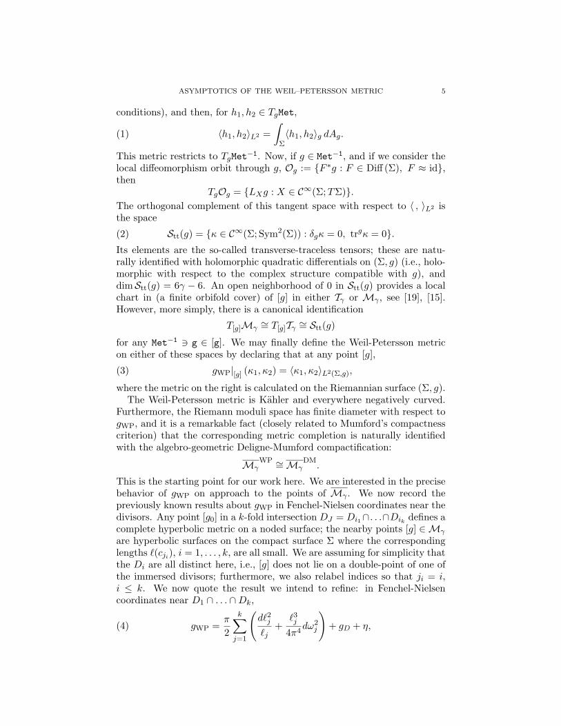
conditions), and then, for h1, h2 ∈ TgMet,
(1) 〈h1, h2〉L2 =∫
Σ〈h1, h2〉g dAg.
This metric restricts to TgMet−1. Now, if g ∈ Met−1, and if we consider thelocal diffeomorphism orbit through g, Og := F ∗g : F ∈ Diff (Σ), F ≈ id,then
TgOg = LXg : X ∈ C∞(Σ;TΣ).The orthogonal complement of this tangent space with respect to 〈 , 〉L2 isthe space
(2) Stt(g) = κ ∈ C∞(Σ; Sym2(Σ)) : δgκ = 0, trgκ = 0.Its elements are the so-called transverse-traceless tensors; these are natu-rally identified with holomorphic quadratic differentials on (Σ, g) (i.e., holo-morphic with respect to the complex structure compatible with g), anddimStt(g) = 6γ − 6. An open neighborhood of 0 in Stt(g) provides a localchart in (a finite orbifold cover) of [g] in either Tγ or Mγ , see [19], [15].However, more simply, there is a canonical identification
T[g]Mγ∼= T[g]Tγ
∼= Stt(g)
for any Met−1 3 g ∈ [g]. We may finally define the Weil-Petersson metricon either of these spaces by declaring that at any point [g],
(3) gWP|[g] (κ1, κ2) = 〈κ1, κ2〉L2(Σ,g),
where the metric on the right is calculated on the Riemannian surface (Σ, g).The Weil-Petersson metric is Kahler and everywhere negatively curved.
Furthermore, the Riemann moduli space has finite diameter with respect togWP, and it is a remarkable fact (closely related to Mumford’s compactnesscriterion) that the corresponding metric completion is naturally identifiedwith the algebro-geometric Deligne-Mumford compactification:
MγWP ∼= Mγ
DM.
This is the starting point for our work here. We are interested in the precisebehavior of gWP on approach to the points of Mγ . We now record thepreviously known results about gWP in Fenchel-Nielsen coordinates near thedivisors. Any point [g0] in a k-fold intersection DJ = Di1∩. . .∩Dik defines acomplete hyperbolic metric on a noded surface; the nearby points [g] ∈Mγ
are hyperbolic surfaces on the compact surface Σ where the correspondinglengths `(cji), i = 1, . . . , k, are all small. We are assuming for simplicity thatthe Di are all distinct here, i.e., [g] does not lie on a double-point of one ofthe immersed divisors; furthermore, we also relabel indices so that ji = i,i ≤ k. We now quote the result we intend to refine: in Fenchel-Nielsencoordinates near D1 ∩ . . . ∩Dk,
(4) gWP =π
2
k∑j=1
(d`2j`j
+`3j
4π4dω2
j
)+ gD + η,
6 R. MAZZEO AND J. SWOBODA
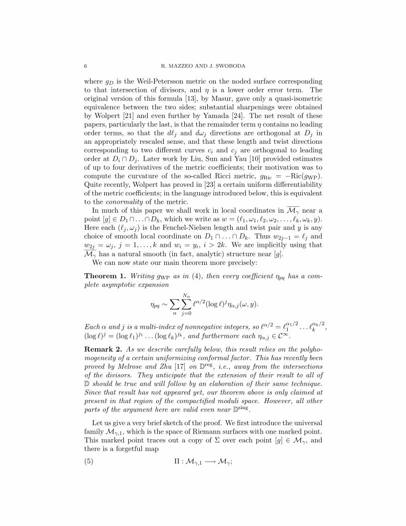
where gD is the Weil-Petersson metric on the noded surface correspondingto that intersection of divisors, and η is a lower order error term. Theoriginal version of this formula [13], by Masur, gave only a quasi-isometricequivalence between the two sides; substantial sharpenings were obtainedby Wolpert [21] and even further by Yamada [24]. The net result of thesepapers, particularly the last, is that the remainder term η contains no leadingorder terms, so that the d`j and dωj directions are orthogonal at Dj inan appropriately rescaled sense, and that these length and twist directionscorresponding to two different curves ci and cj are orthogonal to leadingorder at Di ∩Dj . Later work by Liu, Sun and Yau [10] provided estimatesof up to four derivatives of the metric coefficients; their motivation was tocompute the curvature of the so-called Ricci metric, gRic = −Ric(gWP).Quite recently, Wolpert has proved in [23] a certain uniform differentiabilityof the metric coefficients; in the language introduced below, this is equivalentto the conormality of the metric.
In much of this paper we shall work in local coordinates in Mγ near apoint [g] ∈ D1∩ . . .∩Dk, which we write as w = (`1, ω1, `2, ω2, . . . , `k, ωk, y).Here each (`j , ωj) is the Fenchel-Nielsen length and twist pair and y is anychoice of smooth local coordinate on D1 ∩ . . . ∩ Dk. Thus w2j−1 = `j andw2j = ωj , j = 1, . . . , k and wi = yi, i > 2k. We are implicitly using thatMγ has a natural smooth (in fact, analytic) structure near [g].
We can now state our main theorem more precisely:
Theorem 1. Writing gWP as in (4), then every coefficient ηpq has a com-plete asymptotic expansion
ηpq ∼∑α
Nα∑j=0
`α/2(log `)jηα,j(ω, y).
Each α and j is a multi-index of nonnegative integers, so `α/2 = `α1/21 . . . `
αk/2k ,
(log `)j = (log `1)j1 . . . (log `k)jk , and furthermore each ηα,j ∈ C∞.
Remark 2. As we describe carefully below, this result relies on the polyho-mogeneity of a certain uniformizing conformal factor. This has recently beenproved by Melrose and Zhu [17] on Dreg, i.e., away from the intersectionsof the divisors. They anticipate that the extension of their result to all ofD should be true and will follow by an elaboration of their same technique.Since that result has not appeared yet, our theorem above is only claimed atpresent in that region of the compactified moduli space. However, all otherparts of the argument here are valid even near Dsing.
Let us give a very brief sketch of the proof. We first introduce the universalfamily Mγ,1, which is the space of Riemann surfaces with one marked point.This marked point traces out a copy of Σ over each point [g] ∈ Mγ , andthere is a forgetful map
(5) Π : Mγ,1 −→Mγ ;
ASYMPTOTICS OF THE WEIL–PETERSSON METRIC 7
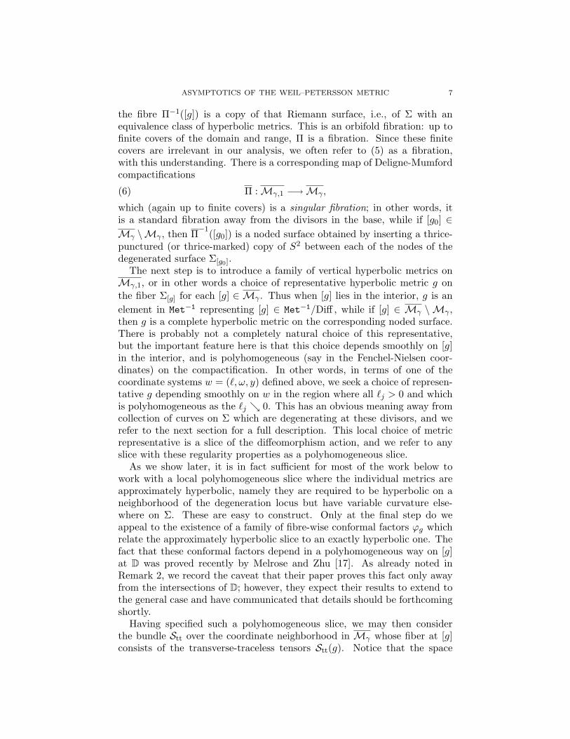
the fibre Π−1([g]) is a copy of that Riemann surface, i.e., of Σ with anequivalence class of hyperbolic metrics. This is an orbifold fibration: up tofinite covers of the domain and range, Π is a fibration. Since these finitecovers are irrelevant in our analysis, we often refer to (5) as a fibration,with this understanding. There is a corresponding map of Deligne-Mumfordcompactifications
(6) Π : Mγ,1 −→Mγ ,
which (again up to finite covers) is a singular fibration; in other words, itis a standard fibration away from the divisors in the base, while if [g0] ∈Mγ \Mγ , then Π−1([g0]) is a noded surface obtained by inserting a thrice-punctured (or thrice-marked) copy of S2 between each of the nodes of thedegenerated surface Σ[g0].
The next step is to introduce a family of vertical hyperbolic metrics onMγ,1, or in other words a choice of representative hyperbolic metric g onthe fiber Σ[g] for each [g] ∈ Mγ . Thus when [g] lies in the interior, g is anelement in Met−1 representing [g] ∈ Met−1/Diff , while if [g] ∈ Mγ \ Mγ ,then g is a complete hyperbolic metric on the corresponding noded surface.There is probably not a completely natural choice of this representative,but the important feature here is that this choice depends smoothly on [g]in the interior, and is polyhomogeneous (say in the Fenchel-Nielsen coor-dinates) on the compactification. In other words, in terms of one of thecoordinate systems w = (`, ω, y) defined above, we seek a choice of represen-tative g depending smoothly on w in the region where all `j > 0 and whichis polyhomogeneous as the `j 0. This has an obvious meaning away fromcollection of curves on Σ which are degenerating at these divisors, and werefer to the next section for a full description. This local choice of metricrepresentative is a slice of the diffeomorphism action, and we refer to anyslice with these regularity properties as a polyhomogeneous slice.
As we show later, it is in fact sufficient for most of the work below towork with a local polyhomogeneous slice where the individual metrics areapproximately hyperbolic, namely they are required to be hyperbolic on aneighborhood of the degeneration locus but have variable curvature else-where on Σ. These are easy to construct. Only at the final step do weappeal to the existence of a family of fibre-wise conformal factors ϕg whichrelate the approximately hyperbolic slice to an exactly hyperbolic one. Thefact that these conformal factors depend in a polyhomogeneous way on [g]at D was proved recently by Melrose and Zhu [17]. As already noted inRemark 2, we record the caveat that their paper proves this fact only awayfrom the intersections of D; however, they expect their results to extend tothe general case and have communicated that details should be forthcomingshortly.
Having specified such a polyhomogeneous slice, we may then considerthe bundle Stt over the coordinate neighborhood in Mγ whose fiber at [g]consists of the transverse-traceless tensors Stt(g). Notice that the space
8 R. MAZZEO AND J. SWOBODA
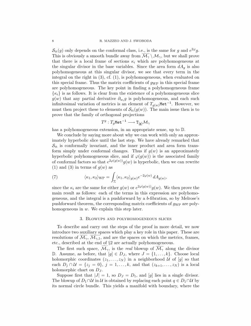
Stt(g) only depends on the conformal class, i.e., is the same for g and e2ϕg.This is obviously a smooth bundle away from Mγ \Mγ , but we shall provethat there is a local frame of sections κi which are polyhomogeneous atthe singular divisor in the base variables. Since the area form dAg is alsopolyhomogeneous at this singular divisor, we see that every term in theintegral on the right in (3), cf. (1), is polyhomogeneous, when evaluated onthis special frame. Thus the matrix coefficients of gWP in this special frameare polyhomogeneous. The key point in finding a polyhomogeneous frameκi is as follows. It is clear from the existence of a polyhomogeneous sliceg(w) that any partial derivative ∂wig is polyhomogeneous, and each suchinfinitesimal variation of metrics is an element of Tg(w)Met
−1. However, wemust then project these to elements of Stt(g(w)). The main issue then is toprove that the family of orthogonal projections
T g : TgMet−1 −→ T[g]Mγ
has a polyhomogeneous extension, in an appropriate sense, up to D.We conclude by saying more about why we can work with only an approx-
imately hyperbolic slice until the last step. We have already remarked thatStt is conformally invariant, and the inner product and area form trans-form simply under conformal changes. Thus if g(w) is an approximatelyhyperbolic polyhomogeneous slice, and if ϕ(g(w)) is the associated familyof conformal factors so that e2ϕ(g(w))g(w) is hyperbolic, then we can rewrite(1) and (3) in terms of g(w) as
(7) 〈κ1, κ2〉WP =∫
Σ〈κ1, κ2〉g(w)e
−2ϕ(w) dAg(w),
since the κi are the same for either g(w) or e2ϕ(g(w))g(w). We then prove themain result as follows: each of the terms in this expression are polyhomo-geneous, and the integral is a pushforward by a b-fibration, so by Melrose’spushforward theorem, the corresponding matrix coefficients of gWP are poly-homogeneous in w. We explain this step later.
3. Blowups and polyhomogeneous slices
To describe and carry out the steps of the proof in more detail, we nowintroduce two auxiliary spaces which play a key role in this paper. These areresolutions of Mγ , Mγ,1, and are the spaces on which the metrics, frames,etc., described at the end of §2 are actually polyhomogeneous.
The first such space, Mγ , is the real blowup of Mγ along the divisorD. Assume, as before, that [g] ∈ DJ , where J = 1, . . . , k. Choose localholomorphic coordinates (z1, . . . , zN ) in a neighborhood U of [g] so thateach Dj ∩ U = zj = 0, j = 1, . . . , k, and that (zk+1, . . . , zN ) is a localholomorphic chart on DJ .
Suppose first that |J | = 1, so DJ = D1, and [g] lies in a single divisor.The blowup of D1∩U in U is obtained by replacing each point q ∈ D1∩U byits normal circle bundle. This yields a manifold with boundary, where the
ASYMPTOTICS OF THE WEIL–PETERSSON METRIC 9
boundary is the total space of a circle bundle over D1 ∩ U . More generally,when |J | > 1, this process is carried out along each one of the Dj ∩ U , andit is clear from the fact that the Dj meet with simple normal crossings thatthe blowups in the different divisors are independent from one another. Thepart of the blowup over each intersection locus DJ is a (S1)|J | bundle. Thisconstruction is well-defined globally and defines a manifold with cornerswhich we call Mγ . To be in accord with current usage, this space is actuallynot quite a manifold with corners for the simple reason that some of theboundary hypersurfaces intersect themselves. Since our considerations arelocal on Mγ , we may overlook this point, and for simplicity we may assumethat we are working on a manifold with corners.
The interiors of the boundary hypersurfaces of Mγ are S1 bundles overDreg, the set of points q ∈ D which lie on only one divisor, and away fromdouble-points. The codimension k corners are (S1)k bundles over the ap-propriate intersections of divisors DJ . Altogether, we write
Mγ = [Mγ ; D].
This space has boundary hypersurfacesHj , j = 1, . . . , N , each correspondingto one of the divisors Dj , as well as corners corresponding to the variousintersections of the Dj . We denote by β the blowdown map Mγ →Mγ .
It is worth noting that the local holomorphic coordinates used here arenot directly comparable to Fenchel-Nielsen coordinates, i.e., while we mayset y = (zk+1, . . . , zN ), it is not the case that each (`j , ωj) is a functionof <zj ,=zj . Nonetheless, the fibres β−1([g]) for [g] ∈ D are well-defined.In fact, defining the polar coordinates |zj |, arg zj , then both of the setsof coordinates (|z|1, arg z1, . . . , |z|k, arg zk, y) and (`1, ω1, . . . , `k, ωk, y) lift tosmooth (actually, real analytic) coordinate systems on Mγ , and these aresmoothly (real analytically) equivalent.
We next consider the analogous construction for the compactified univer-sal family Mγ,1. As noted earlier, up to finite covers, there is a singularfibration Π : Mγ,1 → Mγ , and we wish to define a manifold with cornersobtained by blowing up certain submanifolds of Mγ,1 so that Π lifts to amap
Π : Mγ,1 −→ Mγ
which is a b-fibration between manifolds with corners. To carry out thisconstruction, we first blow down the noded S2 components of the singularfibres Π−1([g0]) inMγ,1; thus we replace these singular fibres by the union ofnoded Riemann surfaces which correspond to the complete hyperbolic metricg0. The resulting space (Mγ,1)′ is the true universal family of Mγ . (Wecould, of course, have bypassed the Deligne-Mumford compactification ofMγ,1 and proceeded directly to this smaller compactification.) The next stepis to lift this singular fibration via the blowdown map β : (Mγ,1)′ → Mγ ;the final step is to blow up the lifts of the nodes of these singular fibres inthe total space. The resulting space is denoted Mγ,1.
10 R. MAZZEO AND J. SWOBODA
It is more transparent to describe all of this in local coordinates. Forsimplicity, consider this first near Dreg. Use the (lifted) Fenchel-Nielsencoordinates (`, ω, y) on Mγ as well as local coordinates (τ, θ) on a neigh-borhood C of the appropriate curve c ⊂ Σ which degenerates at [g0]. Wesuppose that the local choice of approximately hyperbolic metrics g on eachfiber of Π is adapted to these coordinates in the sense that C is the opencylinder C = (−1, 1)τ × S1
θ and
(8) g|C =dτ2
τ2 + `2+ (τ2 + `2) dθ2.
Note that (8) is indeed a hyperbolic metric and can be reduced to the morefamiliar form
dt2 + `2 cosh2(t) dθ2
by the change of coordinates t = arcsinh τ/`. These cylindrical coordinatesextend to the fibers of (Mγ,1)′ over D, but become dependent at the preim-age of the nodal set ` = τ = 0. This preimage has coordinates y, ω, θ,and its blowup reduces to the blowup of (0, 0) in [0, `0)`× (−1, 1)τ , with theremaining coordinates (y, ω, θ) as parameters. Let us use polar coordinates` = ρ sinχ, τ = ρ cosχ, with ρ ≥ 0, χ ∈ [0, π]. Altogether then, (ρ, χ, ω, θ, y)is a coordinate system on Mγ,1. The new face ρ = 0 is called the front face.
It is useful to consider a reduced version of this construction where wereplace the product C × [0, `0)` by its blowup
(9) C = [C × [0, `0); ` = τ = 0].
(In other words, we suppress the coordinates y and ω along the hypersurfaceboundary H of Mγ . As before, the new face is called the front face of C. Aneighborhood of the corresponding region in Mγ,1 is a product C ×S1
ω×Wy,where Wy is a neighborhood of [g0] in D. More generally, near crossingpoints of D, this construction may be carried out independently near eachof the degenerating curves cj .
The space Mγ,1 has two types of boundary hypersurfaces. The first areclosures of the hypersurfaces Hreg
j × (Σ \ cj), where the Hregj are the hyper-
surfaces in Mγ which cover the components of Dreg, and the second are thefaces Fj obtained by blowing up Hreg
j × cj . Because of the self-intersections
of the irreducible components of D, these boundary hypersurfaces of Mγ,1
may self-intersect at their boundaries, and for this reason, Mγ,1 is slightlymore general than a manifold with corners. However, our considerations aresufficiently local that this does not affect anything here, and we shall thinkof this space as a manifold with corners.
The fibration Π : Mγ,1 →Mγ extends to a b-fibration
(10) Π : Mγ,1 −→ Mγ .
ASYMPTOTICS OF THE WEIL–PETERSSON METRIC 11
Briefly, a b-fibration is the most useful analogue of a submersion in thesetting of maps between manifolds with corners. We refer to [16] for theprecise definition of b-fibrations. We appeal to this structure only onceagain, at the very end of this paper. The preimage of a point q in theinterior of Mγ is the compact surface Σ. If q ∈ Hreg
j , then Π−1(q) is aunion of the bordered surface obtained by adding the boundary curves toΣ \ cj and the cylinder [−1, 1] × S1, which is the new face created by thefinal blowup. We also define the vertical tangent bundle T verMγ,1. Its fibresare the tangent planes to the fibres Π−1(q) for q in the interior; over theboundary, however, these fibres are ‘broken’, so the vertical tangent spaceis either the tangent plane to the noded degeneration of Σ, or else to thetangent space of C.
One of the key properties of this fibration is that the family of hyperbolicmetrics gq on the vertical tangent bundle extends naturally to a (degenerate)fibrewise metric on Mγ,1. Over the boundaries of Mγ,1, these vertical hy-perbolic metrics are either the complete finite area hyperbolic metrics, overthe noded degenerations of Σ, or else the complete (infinite area) hyperbolicmetric
dT 2
1 + T 2+ (1 + T 2)dθ2
on the front face of C. Melrose and Zhu [17] prove the following
Proposition 3 ([17]). The family of metrics g(w) on Σ over the interior ofMγ extends to a polyhomogeneous section of the symmetric second power ofthe dual of the vertical tangent bundle of Mγ,1.
Remark 4. As we have already noted, [17] only establishes this polyhomo-geneity near points of Dreg, but not at the intersection locus of the divisors.They expect to complete the proof in that case soon as well.
We conclude this section with a brief explanation for how to make thetranslation between the results in [17] and what is needed here. We beginwith a polyhomogeneous family of approximately hyperbolic metrics g(w)and then find the conformal factor ϕ(w) such that e2ϕ(w)g(w) is hyperbolic.The family g(w) has been constructed to be polyhomogeneous. We indicatenow why the main theorem of [17] shows that ϕ(w) is as well.
The notation in [17] is as follows. The annulus A is identified with thequadric (z, w) : zw = t; for simplicity here we assume that t ∈ R, 0 < t <1/4; this parameter is equivalent to the length parameter `, see below. Weparametrize half of this region by the annulus
√t ≤ |z| ≤ 1/2. The family
of hyperbolic metrics here is given as(π log |z|
log tcsc
π log |z|log t
)2 |dz|2
|z|2(log |z|)2.
12 R. MAZZEO AND J. SWOBODA
This agrees with (8) upon making the substitutions
` =π
| log t|,
τ
`= cot
`
| log |z||.
In [17], the radial variable |z| is replaced by 1/| log |z||, so this change ofvariables shows that polyhomogeneity (and indeed log smoothness) in thisnew logarithmic variable, as proved in [17], is equivalent to polyhomogeneity(log smoothness) in τ .
4. Global analysis and Mγ
We now recall some standard facts about deformations of hyperbolic met-rics on surfaces. The point of view adopted here is the one promoted byTromba [19], and is the specialization to this low dimension of the deforma-tion theory of Einstein metrics.
4.1. Curvature equations and Bianchi gauge. Consider the operatorwhich assigns to a metric its Gauss curvature: g 7→ Kg. This is a secondorder nonlinear differential operator, and since Ricg = Kgg in dimension2, metrics of constant curvature are the same as Einstein metrics in thissetting.
Let (Σ2, g0) be a closed surface where Kg0 ≡ −1. Nearby hyperbolicmetrics correspond to solutions of
(11) S2(Σ, T ∗Σ) 3 h 7→ Eg0(h) := (Kg0+h + 1) · (g0 + h) = 0
with h suitably small. The nonlinear operator Eg0 is called the Einstein op-erator. Since Σ is compact, we can let Eg0 act between appropriate Sobolevor Holder spaces, but for simplicity we do not specify the function spacesprecisely until necessary.
The operator Eg0 is not elliptic because it is invariant under the infinite-dimensional group Diff(Σ) of diffeomorphisms of Σ. For any metric g, thetangent space of the Diff(Σ) orbit through g consists of all symmetric 2-tensors of the form LXg, where X is a vector field on Σ, or equivalently, as(δg)∗ω, where ω is the 1-form metrically dual to X. Here δg : S2(Σ, T ∗Σ) →Ω1(Σ) is the divergence operator and (δg0)∗ is its adjoint; in local coordi-nates,
((δg)∗ω)ij =12(ωi;j + ωj;i).
Note that trg(δg)∗ = −δg : Ω1 → Ω0, where δg : Ω1(Σ) → Ω0(Σ) is thestandard codifferential. The conformal Killing operator is the projection of(δg)∗ onto its trace-free part:
Dgω := (δg)∗ω +12δg(ω)g : Ω1(Σ) → S2
0(Σ, T ∗Σ).
This is the adjoint of δg : S20(Σ, T ∗Σ) → Ω1(Σ). It follows from all this that
the nullspace of δg on S2(Σ, T ∗Σ) equals the L2-orthogonal complement
ASYMPTOTICS OF THE WEIL–PETERSSON METRIC 13
of the tangent space of the diffeomorphism orbit passing through g, andfurthermore that the system
h 7→ (Eg(h), δg(h))
is elliptic. It is convenient to consider instead the single operator
Ng(h) := Eg(h) + (δg+h)∗Bg(h) = (Kg+h + 1)(g + h) + (δg+h)∗Bg(h),
where
(12) h 7→ Bg(h) := δg(h) +12dtrgh
is the Bianchi operator. We say that h is in Bianchi gauge if Bg(h) = 0.Clearly, if Eg(h) = 0 and Bg(h) = 0, then Ng(h) = 0. The converse, whichis due to Biquard, is true as well.
Proposition 5. Suppose that g0 is hyperbolic. If h ∈ S2(Σ, T ∗Σ) is suffi-ciently small and Ng0(h) = 0, then g0 + h has constant Gauss curvature −1and Bg0(h) = 0.
Before recalling Biquard’s proof, recall that if h = fg is pure trace, then
(13) Bg(fg) = δg(fg) +12dtrg(fg) = −df + df = 0.
Thus applying Bg+h to Ng(h) yields
(14) Bg+h(Eg(h)) = Bg+h(δg+h)∗Bg(h) = 0.
For any metric, write
(15) P g := Bg (δg)∗ : Ω1(Σ) → Ω1(Σ);
by a standard Weitzenbock identity,
(16) P g =12(∆g − 2Kg),
where ∆g is the Hodge Laplacian on 1-forms.
Proof. It suffices to establish that, if g = g0 is hyperbolic, then ω = Bg0(h) =0. By (14), P g0+hω = 0, or equivalently, by (16),
〈2P g0+hω, ω〉 = ‖∇g0+hω‖2 − 2Kg0+h‖ω‖2 = 0.
However, since Kg0 = −1, then if h is sufficiently small, Kg0+h < 0. Weconclude that ω = 0, and thus Eg0(h) = 0, as desired.
14 R. MAZZEO AND J. SWOBODA
4.2. Linearized curvature operators. The linearizations of the curva-ture operators above are not hard to compute. As before, assume through-out that Kg0 ≡ −1. If h = h0 + fg0 is the decomposition into trace-free andpure-trace parts, then
(17) DKg0(h) = (12∆g0 + 1)f +
12δg0δg0h0.
We see directly from this that
DEg0(k) =((12∆g0 + 1)f +
12δg0δg0h0
)g0,
and furthermore,
(18) DNg0(h) := Lg0(h) =12(∇∗∇− 2)h0 +
(12(∆g + 2)f
)g.
We call Lg0 the linearized Bianchi-gauged Einstein operator. Note finallythat by differentiating the identity Bg+hNg(h) = P g+hBg(h) at h = 0, weobtain
BgLg = P gBg.
4.3. Transverse-traceless tensors. A key object in this paper is the spaceStt = Stt(g0) of transverse-traceless tensors on the surface Σ with respect tothe metric g0; by definition, this is the nullspace of Lg0 . This space representsthe tangent space of Mγ at g0 and depends only on the conformal class [g0],cf. Proposition 6 below.
Using (18), Lg0(h0 + fg0) = 0 if and only if f = 0 and (∇∗∇− 2)h0 = 0;by (16), the second condition is equivalent to δg0h0 = 0. Therefore
kerLg0 = Stt(g0) = h ∈ S2(Σ, T ∗Σ) | δg0h = 0, trg0h = 0and hence Stt is the tangent space to the submanifold of metrics with con-stant curvature K ≡ −1 in Bianchi gauge with respect to g0. In particular,Stt is orthogonal to the diffeomorphism orbit through g0. It is straightfor-ward to check that since dim Σ = 2, δg0 is elliptic as a map between sectionsof S2
0(Σ, T ∗Σ) and Ω1(Σ), hence dimStt < ∞ and consists of smooth ele-ments. In fact
dimSgtt = 6(γ − 1);
this holds because there is a canonical identification of Stt with the space ofholomorphic quadratic differentials on Σ.
Proposition 6. When dim Σ = 2, Stt is conformally invariant; in otherwords, if g1 = e2ug then
trg1h = 0, δg1h = 0 ⇐⇒ trgh = 0, δgh = 0.
Proof. The first part of the condition is obvious since trg1h = e−2utrgh. Therest follows from the general identity
δg1h = e−2u(δgh+ (trgh)du+ (2− n)ι(∇gu)h),
so since n = 2, if trgh = 0 and δgh = 0, then δg1h = 0, as claimed.
ASYMPTOTICS OF THE WEIL–PETERSSON METRIC 15
4.4. Local deformation theory. It is now standard to deduce some fea-tures of the local deformation theory of hyperbolic metrics. We refer to [15]and [19] for complete proofs.
If (Σ, g0) is a closed hyperbolic surface, as above, we describe the Banachspace structure of all nearby Riemannian metrics g (in the C2,α topology)with Kg = −1, and identify those metrics in this Banach submanifold whichare in a local slice with respect to the action of Diff(Σ).
Write Mhyp for the set of C2,α Riemannian metrics with curvature −1.
Lemma 7. The space Mhyp is a Banach submanifold in C2,αS2(Σ, T ∗Σ).
By the discussion above,
Tg0Mhyp = h ∈ C2,αS2(Σ, T ∗Σ) | DKg0h = 0= h = h0 + fg0 ∈ C2,αS2(Σ, T ∗Σ) | trg0h0 = 0, (∆g0 + 2)f + δg0h0 = 0.
We now impose the gauge condition.
Lemma 8. There is a constant ε depending on g0 such that the intersectionof
Sg0,ε := Mhyp ∩ g0 + h : Bg0h = 0, ‖h‖2,α < εwith the orbit of Diff3,α(Σ) is transverse at g0. The space Sg0,ε is identifiedwith the space of solutions h to Ng0(h) = 0 with ‖h‖2,α < ε, and its tangentspace at g0 equals Stt(g0).
There is also a local slice theorem.
Theorem 9. There is a positive constant ε depending on g0 and a neigh-borhood U of id in Diff3,α(Σ) such that the map
U × Sg0,ε 3 (F, h) 7→ F ∗(g0 + h)
is a diffeomorphism onto some neighborhood of g0 in Mhyp.
In fact, since the genus γ > 1, one can show that the action of theentire connected component of the identity of the diffeomorphism groupacts properly.
4.5. The Weil-Petersson metric. We now use this formalism to describethe Weil-Petersson metric.
Let t 7→ gt, |t| < ε, be a smooth path of hyperbolic Riemannian metricsthrough g0. For ε small, then Theorem 9 shows that there exists a uniqueht ∈ S2(Σ, T ∗Σ) such that Ng0(ht) = 0 and ht = F ∗t gt for some diffeomor-phism Ft, so in particular the differential κ := d
dt
∣∣t=0
ht lies in Stt(g0). Wenow compute κ in terms of g = d
dt
∣∣t=0
gt. Indeed, there exists a smooth fam-ily of diffeomorphisms Ft and a smooth family of scalar functions ut suchthat
(19) g0 + ht = F ∗t e2utgt.
16 R. MAZZEO AND J. SWOBODA
Write X = ddt
∣∣t=0
Ft and u = ddt
∣∣t=0
ut. Differentiating (19) with respect to tat t = 0 yields
(20) κ = LXg0 + 2ug0 + g = (δg0)∗ω + 2u g0 + g,
where X[ = ω ∈ Ω1(Σ) is the 1-form dual to X with respect to g0.We first determine ω as follows. Apply Bg0 to (20) and recall (15), to get
P g0ω = −Bg0 g,
since Bg0κ = 0. By (16), P g0 is invertible, so denoting its inverse by Gg0 ,we can write
ω = −Gg0Bg0 g.
Finally, with πg0 : S2(Σ, T ∗Σ) → S20(Σ, T ∗Σ) the orthogonal projection onto
trace-free tensors, we obtain that
κ = −πg0(δg0)∗Gg0Bg0 g + πg0 g.
In other words, κ = T g0 g, where the L2-orthogonal projection L2S20(Σ, T ∗Σ) →
Stt is given by
(21) T g0 = πg0 (id− (δg0)∗Gg0Bg0) .
This now gives the formulæ for the Weil-Petersson norm and inner prod-uct:
(22) ‖κ‖2WP = ‖T g0 g‖2L2(Σ,dAg0 ), 〈κ1, κ2〉WP = 〈T g0 g1, Tg0 g2〉L2(Σ,dAg0 ).
Our goal in the remainder of this paper is to analyze these expressionsnear the singular divisors of Mγ . Our main result is that there is a basisof sections of Stt which depends in a polyhomogeneous manner on g0. Themain issue is to prove that the operator Gg0 is polyhomogeneous in g0.
5. Hyperbolic cylinders
The first step in this analysis is to study this problem for a model familyof finite hyperbolic cylinders (C, g`) where the length ` of the central geodesicdecreases to 0. We have already described these metrics in (8) above, andwe note here that either component of the boundary ∂C = τ = ±1 is atdistance arcsinh(1/`) ∼ | log( `
2)| from the central geodesic τ = 0.We consider here the family of inverses Gg` to the operators P g` on C and
shall prove that it is polyhomogeneous in a particular sense as ` 0. Thisanalysis is explicit and we use it later to construct a parametrix for P g onfamilies of degenerating compact hyperbolic surfaces.
It is here that the blowup C of C × [0, `0), which we introduced in (9),becomes important. Indeed, the family Gg` has a rather complicated struc-ture at ` = 0; the most precise description of this behaviour, which wasstudied carefully in [1], is that it is polyhomogeneous on a space obtainedby a sequence of blowups of C×C× [0, `0). Fortunately we do not need all ofthis, and shall only require a much weaker form of this, which we can provedirectly. Namely, we show that if the family of 1-forms h` on C × [0, `0)
ASYMPTOTICS OF THE WEIL–PETERSSON METRIC 17
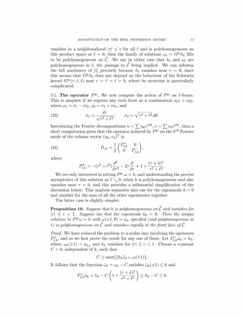
vanishes in a neighbourhood |τ | ≤ c for all ` and is polyhomogeneous onthis product space at ` = 0, then the family of solutions ω` = Gg`h` liftsto be polyhomogeneous on C. We say in either case that h` and ω` arepolyhomogeneous in `, the passage to C being implied. We can sidestepthe full machinery of [1] precisely because h` vanishes near τ = 0, sincethis means that Gg`h` does not depend on the behaviour of the Schwartzkernel Gg`(τ, τ , `) near τ = τ = ` = 0, where its structure is particularlycomplicated.
5.1. The operator P g`. We now compute the action of P g` on 1-forms.This is simplest if we express any such form as a combination uρ1 + vρ2,where ρ1 = σ1 − iσ2, ρ2 = σ1 + iσ2, and
(23) σ1 =dτ√τ2 + `2
, σ2 =√τ2 + `2 dθ.
Introducing the Fourier decompositions u =∑uke
ikθ, v =∑vke
ikθ, then ashort computation gives that the operator induced by P g` on the kth Fouriermode of the column vector (uk, vk)T is
(24) P`,k =12
(P+
`,k 00 P−`,k
),
where
P±`,k = −(τ2 + `2)d2
dτ2− 2τ
d
dτ+ 1 +
(τ ± k)2
τ2 + `2.
We are only interested in solving P g` ω = h, and understanding the preciseasymptotics of this solution as ` 0, when h is polyhomogeneous and alsovanishes near τ = 0, and this provides a substantial simplification of thediscussion below. This analysis separates into one for the eigenmode k = 0and another for the sum of all the other eigenmodes together.
The latter case is slightly simpler.
Proposition 10. Suppose that h is polyhomogeneous on C and vanishes for|τ | ≤ c < 1. Suppose too that the eigenmode h0 = 0. Then the uniquesolution to P g`ω = h with ω(±1, θ) = η± specified (and polyhomogenous in`) is polyhomogeneous on C and vanishes rapidly at the front face of C.
Proof. We have reduced the problem to a scalar one, involving the operatorsP±`,k, and so we first prove the result for any one of these. Let P+
`,kωk = hk,where ωk(±1) = η±k
and hk vanishes for |τ | ≤ c < 1. Choose a constantC > 0, independent of k, such that
C ≥ max‖hk‖L∞ , ω(±1).
It follows that the function ωk = ωk − C satisfies ωk(±1) ≤ 0 and
P+`,kωk = hk − C
(1 +
(τ + k)2
τ2 + `2
)≤ hk − C ≤ 0.
18 R. MAZZEO AND J. SWOBODA
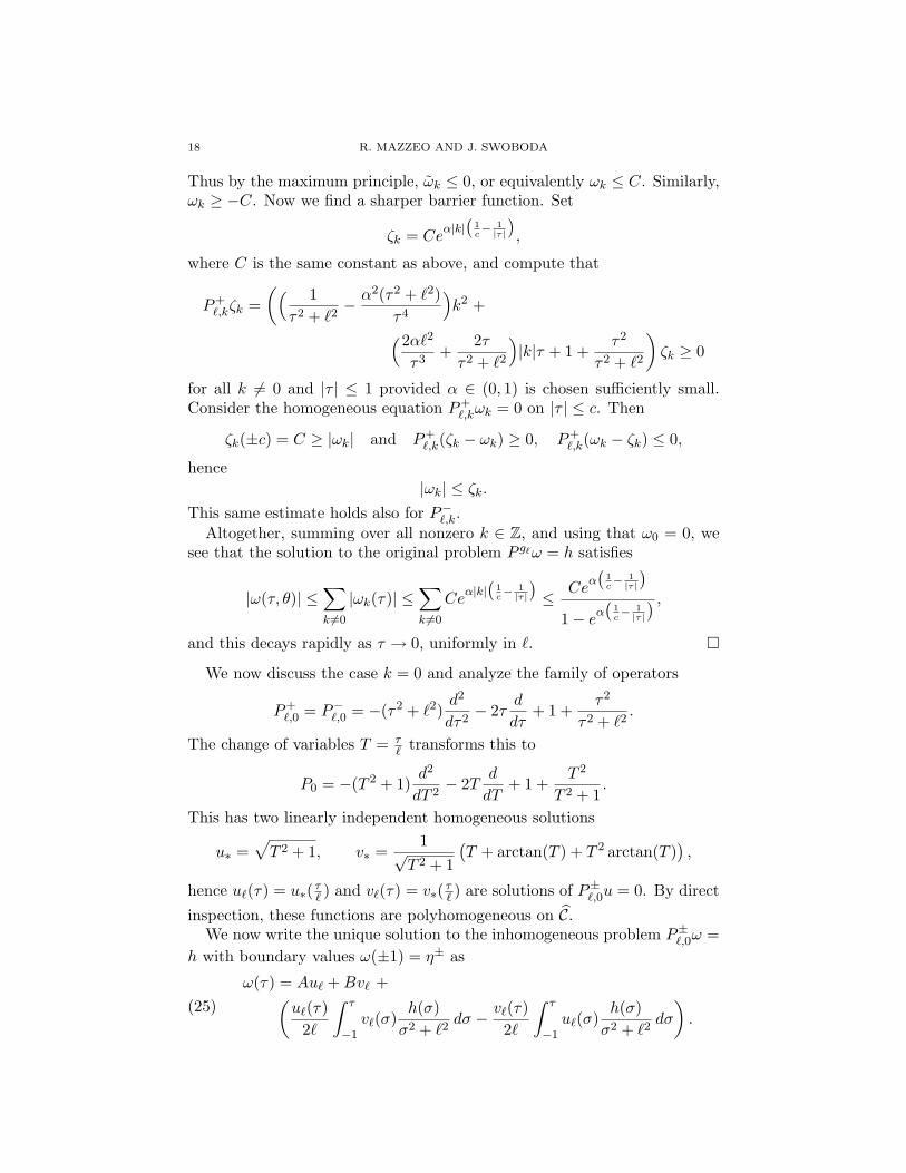
Thus by the maximum principle, ωk ≤ 0, or equivalently ωk ≤ C. Similarly,ωk ≥ −C. Now we find a sharper barrier function. Set
ζk = Ceα|k|(
1c− 1|τ |
),
where C is the same constant as above, and compute that
P+`,kζk =
(( 1τ2 + `2
− α2(τ2 + `2)τ4
)k2 +(2α`2
τ3+
2ττ2 + `2
)|k|τ + 1 +
τ2
τ2 + `2
)ζk ≥ 0
for all k 6= 0 and |τ | ≤ 1 provided α ∈ (0, 1) is chosen sufficiently small.Consider the homogeneous equation P+
`,kωk = 0 on |τ | ≤ c. Then
ζk(±c) = C ≥ |ωk| and P+`,k(ζk − ωk) ≥ 0, P+
`,k(ωk − ζk) ≤ 0,
hence|ωk| ≤ ζk.
This same estimate holds also for P−`,k.Altogether, summing over all nonzero k ∈ Z, and using that ω0 = 0, we
see that the solution to the original problem P g`ω = h satisfies
|ω(τ, θ)| ≤∑k 6=0
|ωk(τ)| ≤∑k 6=0
Ceα|k|(
1c− 1|τ |
)≤ Ce
α(
1c− 1|τ |
)1− e
α(
1c− 1|τ |
) ,and this decays rapidly as τ → 0, uniformly in `.
We now discuss the case k = 0 and analyze the family of operators
P+`,0 = P−`,0 = −(τ2 + `2)
d2
dτ2− 2τ
d
dτ+ 1 +
τ2
τ2 + `2.
The change of variables T = τ` transforms this to
P0 = −(T 2 + 1)d2
dT 2− 2T
d
dT+ 1 +
T 2
T 2 + 1.
This has two linearly independent homogeneous solutions
u∗ =√T 2 + 1, v∗ =
1√T 2 + 1
(T + arctan(T ) + T 2 arctan(T )
),
hence u`(τ) = u∗( τ` ) and v`(τ) = v∗( τ
` ) are solutions of P±`,0u = 0. By direct
inspection, these functions are polyhomogeneous on C.We now write the unique solution to the inhomogeneous problem P±`,0ω =
h with boundary values ω(±1) = η± as
ω(τ) = Au` +Bv` +(u`(τ)
2`
∫ τ
−1v`(σ)
h(σ)σ2 + `2
dσ − v`(τ)2`
∫ τ
−1u`(σ)
h(σ)σ2 + `2
dσ
).
(25)
ASYMPTOTICS OF THE WEIL–PETERSSON METRIC 19
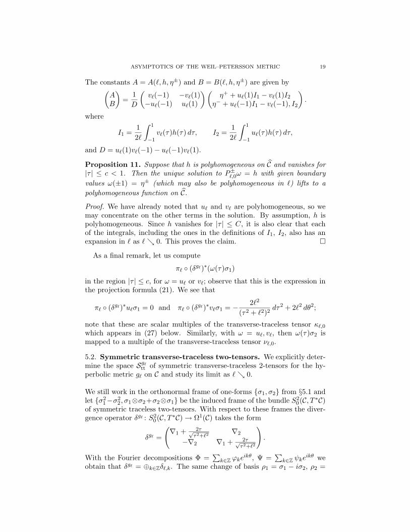
The constants A = A(`, h, η±) and B = B(`, h, η±) are given by(AB
)=
1D
(v`(−1) −v`(1)−u`(−1) u`(1)
)(η+ + u`(1)I1 − v`(1)I2
η− + u`(−1)I1 − v`(−1), I2
).
where
I1 =12`
∫ 1
−1v`(τ)h(τ) dτ, I2 =
12`
∫ 1
−1u`(τ)h(τ) dτ,
and D = u`(1)v`(−1)− u`(−1)v`(1).
Proposition 11. Suppose that h is polyhomogeneous on C and vanishes for|τ | ≤ c < 1. Then the unique solution to P±`,0ω = h with given boundaryvalues ω(±1) = η± (which may also be polyhomogeneous in `) lifts to apolyhomogeneous function on C.
Proof. We have already noted that u` and v` are polyhomogeneous, so wemay concentrate on the other terms in the solution. By assumption, h ispolyhomogeneous. Since h vanishes for |τ | ≤ C, it is also clear that eachof the integrals, including the ones in the definitions of I1, I2, also has anexpansion in ` as ` 0. This proves the claim.
As a final remark, let us compute
π` (δg`)∗(ω(τ)σ1)
in the region |τ | ≤ c, for ω = u` or v`; observe that this is the expression inthe projection formula (21). We see that
π` (δg`)∗u`σ1 = 0 and π` (δg`)∗v`σ1 = − 2`2
(τ2 + `2)2dτ2 + 2`2 dθ2;
note that these are scalar multiples of the transverse-traceless tensor κ`,0
which appears in (27) below. Similarly, with ω = u`, v`, then ω(τ)σ2 ismapped to a multiple of the transverse-traceless tensor ν`,0.
5.2. Symmetric transverse-traceless two-tensors. We explicitly deter-mine the space Sg`
tt of symmetric transverse-traceless 2-tensors for the hy-perbolic metric g` on C and study its limit as ` 0.
We still work in the orthonormal frame of one-forms σ1, σ2 from §5.1 andlet σ2
1−σ22, σ1⊗σ2+σ2⊗σ1 be the induced frame of the bundle S2
0(C, T ∗C)of symmetric traceless two-tensors. With respect to these frames the diver-gence operator δg` : S2
0(C, T ∗C) → Ω1(C) takes the form
δg` =
(∇1 + 2τ√
τ2+`2∇2
−∇2 ∇1 + 2τ√τ2+`2
).
With the Fourier decompositions Φ =∑
k∈Z ϕkeikθ, Ψ =
∑k∈Z ψke
ikθ weobtain that δg` = ⊕k∈Zδ`,k. The same change of basis ρ1 = σ1 − iσ2, ρ2 =
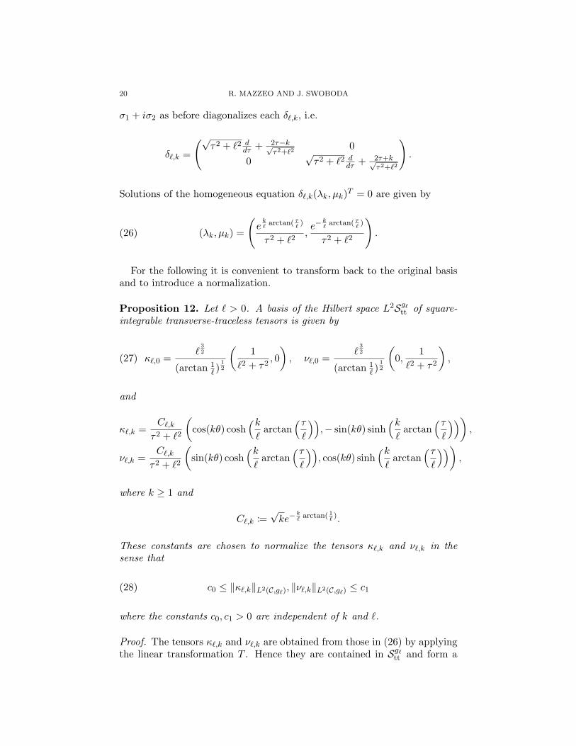
20 R. MAZZEO AND J. SWOBODA
σ1 + iσ2 as before diagonalizes each δ`,k, i.e.
δ`,k =
(√τ2 + `2 d
dτ + 2τ−k√τ2+`2
00
√τ2 + `2 d
dτ + 2τ+k√τ2+`2
).
Solutions of the homogeneous equation δ`,k(λk, µk)T = 0 are given by
(26) (λk, µk) =
(e
k`
arctan( τ`)
τ2 + `2,e−
k`
arctan( τ`)
τ2 + `2
).
For the following it is convenient to transform back to the original basisand to introduce a normalization.
Proposition 12. Let ` > 0. A basis of the Hilbert space L2Sg`tt of square-
integrable transverse-traceless tensors is given by
(27) κ`,0 =`
32
(arctan 1` )
12
(1
`2 + τ2, 0), ν`,0 =
`32
(arctan 1` )
12
(0,
1`2 + τ2
),
and
κ`,k =C`,k
τ2 + `2
(cos(kθ) cosh
(k`
arctan(τ`
)),− sin(kθ) sinh
(k`
arctan(τ`
))),
ν`,k =C`,k
τ2 + `2
(sin(kθ) cosh
(k`
arctan(τ`
)), cos(kθ) sinh
(k`
arctan(τ`
))),
where k ≥ 1 and
C`,k :=√ke−
k`
arctan( 1`).
These constants are chosen to normalize the tensors κ`,k and ν`,k in thesense that
(28) c0 ≤ ‖κ`,k‖L2(C,g`), ‖ν`,k‖L2(C,g`) ≤ c1
where the constants c0, c1 > 0 are independent of k and `.
Proof. The tensors κ`,k and ν`,k are obtained from those in (26) by applyingthe linear transformation T . Hence they are contained in Sg`
tt and form a
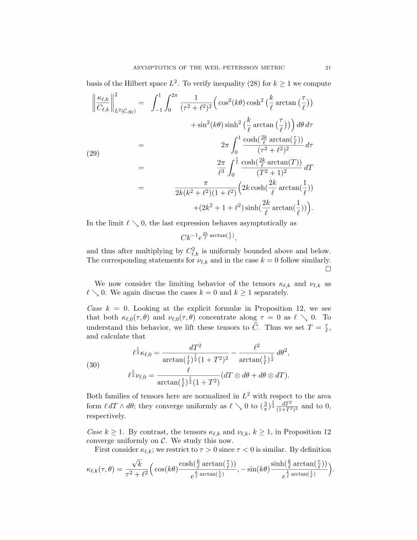
ASYMPTOTICS OF THE WEIL–PETERSSON METRIC 21
basis of the Hilbert space L2. To verify inequality (28) for k ≥ 1 we compute∥∥∥∥ κ`,k
C`,k
∥∥∥∥2
L2(C,g`)
=∫ 1
−1
∫ 2π
0
1(τ2 + `2)2
(cos2(kθ) cosh2
(k`
arctan(τ`
))+sin2(kθ) sinh2
(k`
arctan(τ`
)))dθ dτ
= 2π∫ 1
0
cosh(2k` arctan( τ
` ))(τ2 + `2)2
dτ
=2π`3
∫ 1`
0
cosh(2k` arctan(T ))
(T 2 + 1)2dT
=π
2k(k2 + `2)(1 + `2)
(2k cosh(
2k`
arctan(1`))
+(2k2 + 1 + `2) sinh(2k`
arctan(1`))).
(29)
In the limit ` 0, the last expression behaves asymptotically as
Ck−1e2k`
arctan( 1`),
and thus after multiplying by C2`,k is uniformly bounded above and below.
The corresponding statements for ν`,k and in the case k = 0 follow similarly.
We now consider the limiting behavior of the tensors κ`,k and ν`,k as` 0. We again discuss the cases k = 0 and k ≥ 1 separately.
Case k = 0. Looking at the explicit formulæ in Proposition 12, we seethat both κ`,0(τ, θ) and ν`,0(τ, θ) concentrate along τ = 0 as ` 0. Tounderstand this behavior, we lift these tensors to C. Thus we set T = τ
` ,and calculate that
`12κ`,0 =
dT 2
arctan(1` )
12 (1 + T 2)2
− `2
arctan(1` )
12
dθ2,
`12 ν`,0 =
`
arctan(1` )
12 (1 + T 2)
(dT ⊗ dθ + dθ ⊗ dT ).(30)
Both families of tensors here are normalized in L2 with respect to the areaform ` dT ∧ dθ; they converge uniformly as ` 0 to ( 2
π )12
dT 2
(1+T 2)2and to 0,
respectively.
Case k ≥ 1. By contrast, the tensors κ`,k and ν`,k, k ≥ 1, in Proposition 12converge uniformly on C. We study this now.
First consider κ`,k; we restrict to τ > 0 since τ < 0 is similar. By definition
κ`,k(τ, θ) =
√k
τ2 + `2
(cos(kθ)
cosh(k` arctan( τ
` ))
ek`
arctan( 1`)
,− sin(kθ)sinh(k
` arctan( τ` ))
ek`
arctan( 1`)
).
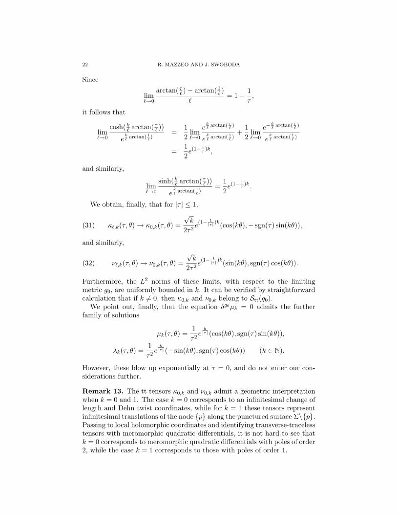
22 R. MAZZEO AND J. SWOBODA
Since
lim`→0
arctan( τ` )− arctan(1
` )`
= 1− 1τ,
it follows that
lim`→0
cosh(k` arctan( τ
` ))
ek`
arctan( 1`)
=12
lim`→0
ek`
arctan( τ`)
ek`
arctan( 1`)
+12
lim`→0
e−k`
arctan( τ`)
ek`
arctan( 1`)
=12e(1−
1τ)k,
and similarly,
lim`→0
sinh(k` arctan( τ
` ))
ek`
arctan( 1`)
=12e(1−
1τ)k.
We obtain, finally, that for |τ | ≤ 1,
(31) κ`,k(τ, θ) → κ0,k(τ, θ) =
√k
2τ2e(1− 1
|τ | )k(cos(kθ),− sgn(τ) sin(kθ)),
and similarly,
(32) ν`,k(τ, θ) → ν0,k(τ, θ) =
√k
2τ2e(1− 1
|τ | )k(sin(kθ), sgn(τ) cos(kθ)).
Furthermore, the L2 norms of these limits, with respect to the limitingmetric g0, are uniformly bounded in k. It can be verified by straightforwardcalculation that if k 6= 0, then κ0,k and ν0,k belong to Stt(g0).
We point out, finally, that the equation δg0µk = 0 admits the furtherfamily of solutions
µk(τ, θ) =1τ2e
k|τ | (cos(kθ), sgn(τ) sin(kθ)),
λk(τ, θ) =1τ2e
k|τ | (− sin(kθ), sgn(τ) cos(kθ)) (k ∈ N).
However, these blow up exponentially at τ = 0, and do not enter our con-siderations further.
Remark 13. The tt tensors κ0,k and ν0,k admit a geometric interpretationwhen k = 0 and 1. The case k = 0 corresponds to an infinitesimal change oflength and Dehn twist coordinates, while for k = 1 these tensors representinfinitesimal translations of the node p along the punctured surface Σ\p.Passing to local holomorphic coordinates and identifying transverse-tracelesstensors with meromorphic quadratic differentials, it is not hard to see thatk = 0 corresponds to meromorphic quadratic differentials with poles of order2, while the case k = 1 corresponds to those with poles of order 1.
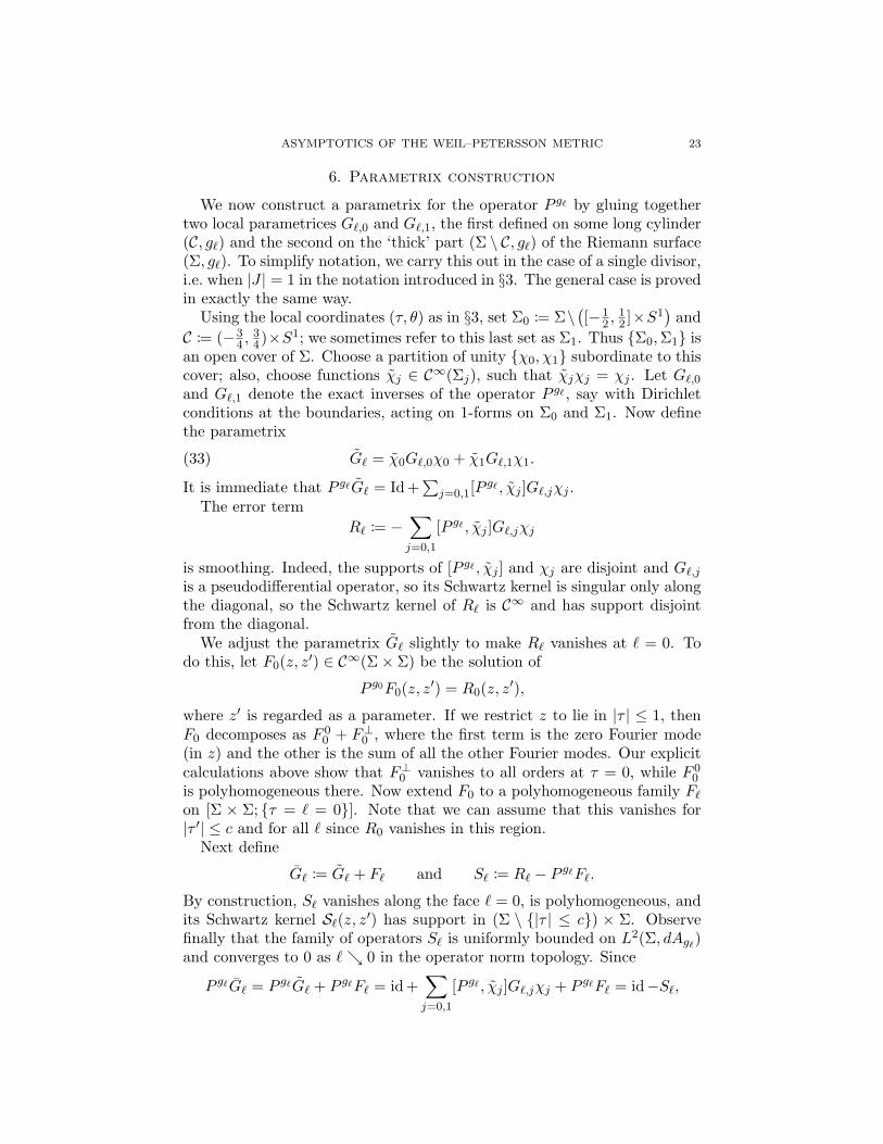
ASYMPTOTICS OF THE WEIL–PETERSSON METRIC 23
6. Parametrix construction
We now construct a parametrix for the operator P g` by gluing togethertwo local parametrices G`,0 and G`,1, the first defined on some long cylinder(C, g`) and the second on the ‘thick’ part (Σ \ C, g`) of the Riemann surface(Σ, g`). To simplify notation, we carry this out in the case of a single divisor,i.e. when |J | = 1 in the notation introduced in §3. The general case is provedin exactly the same way.
Using the local coordinates (τ, θ) as in §3, set Σ0 := Σ\([−1
2 ,12 ]×S1
)and
C := (−34 ,
34)×S1; we sometimes refer to this last set as Σ1. Thus Σ0,Σ1 is
an open cover of Σ. Choose a partition of unity χ0, χ1 subordinate to thiscover; also, choose functions χj ∈ C∞(Σj), such that χjχj = χj . Let G`,0
and G`,1 denote the exact inverses of the operator P g` , say with Dirichletconditions at the boundaries, acting on 1-forms on Σ0 and Σ1. Now definethe parametrix
(33) G` = χ0G`,0χ0 + χ1G`,1χ1.
It is immediate that P g`G` = Id+∑
j=0,1[Pg` , χj ]G`,jχj .
The error termR` := −
∑j=0,1
[P g` , χj ]G`,jχj
is smoothing. Indeed, the supports of [P g` , χj ] and χj are disjoint and G`,j
is a pseudodifferential operator, so its Schwartz kernel is singular only alongthe diagonal, so the Schwartz kernel of R` is C∞ and has support disjointfrom the diagonal.
We adjust the parametrix G` slightly to make R` vanishes at ` = 0. Todo this, let F0(z, z′) ∈ C∞(Σ× Σ) be the solution of
P g0F0(z, z′) = R0(z, z′),
where z′ is regarded as a parameter. If we restrict z to lie in |τ | ≤ 1, thenF0 decomposes as F 0
0 + F⊥0 , where the first term is the zero Fourier mode(in z) and the other is the sum of all the other Fourier modes. Our explicitcalculations above show that F⊥0 vanishes to all orders at τ = 0, while F 0
0
is polyhomogeneous there. Now extend F0 to a polyhomogeneous family F`
on [Σ × Σ; τ = ` = 0]. Note that we can assume that this vanishes for|τ ′| ≤ c and for all ` since R0 vanishes in this region.
Next define
G` := G` + F` and S` := R` − P g`F`.
By construction, S` vanishes along the face ` = 0, is polyhomogeneous, andits Schwartz kernel S`(z, z′) has support in (Σ \ |τ | ≤ c) × Σ. Observefinally that the family of operators S` is uniformly bounded on L2(Σ, dAg`
)and converges to 0 as ` 0 in the operator norm topology. Since
P g`G` = P g`G` + P g`F` = id +∑
j=0,1
[P g` , χj ]G`,jχj + P g`F` = id−S`,
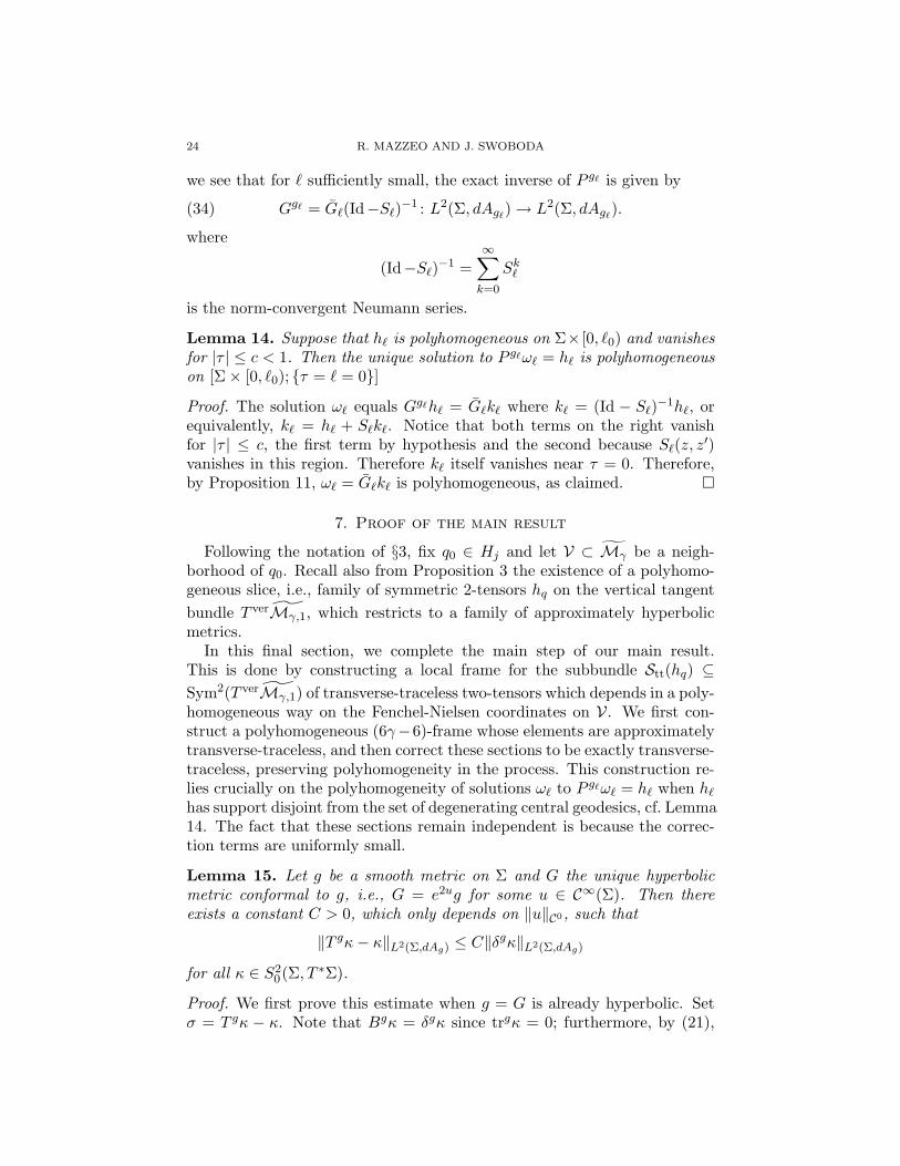
24 R. MAZZEO AND J. SWOBODA
we see that for ` sufficiently small, the exact inverse of P g` is given by
(34) Gg` = G`(Id−S`)−1 : L2(Σ, dAg`) → L2(Σ, dAg`
).
where
(Id−S`)−1 =∞∑
k=0
Sk`
is the norm-convergent Neumann series.
Lemma 14. Suppose that h` is polyhomogeneous on Σ× [0, `0) and vanishesfor |τ | ≤ c < 1. Then the unique solution to P g`ω` = h` is polyhomogeneouson [Σ× [0, `0); τ = ` = 0]
Proof. The solution ω` equals Gg`h` = G`k` where k` = (Id − S`)−1h`, orequivalently, k` = h` + S`k`. Notice that both terms on the right vanishfor |τ | ≤ c, the first term by hypothesis and the second because S`(z, z′)vanishes in this region. Therefore k` itself vanishes near τ = 0. Therefore,by Proposition 11, ω` = G`k` is polyhomogeneous, as claimed.
7. Proof of the main result
Following the notation of §3, fix q0 ∈ Hj and let V ⊂ Mγ be a neigh-borhood of q0. Recall also from Proposition 3 the existence of a polyhomo-geneous slice, i.e., family of symmetric 2-tensors hq on the vertical tangentbundle T verMγ,1, which restricts to a family of approximately hyperbolicmetrics.
In this final section, we complete the main step of our main result.This is done by constructing a local frame for the subbundle Stt(hq) ⊆Sym2(T verMγ,1) of transverse-traceless two-tensors which depends in a poly-homogeneous way on the Fenchel-Nielsen coordinates on V. We first con-struct a polyhomogeneous (6γ−6)-frame whose elements are approximatelytransverse-traceless, and then correct these sections to be exactly transverse-traceless, preserving polyhomogeneity in the process. This construction re-lies crucially on the polyhomogeneity of solutions ω` to P g`ω` = h` when h`
has support disjoint from the set of degenerating central geodesics, cf. Lemma14. The fact that these sections remain independent is because the correc-tion terms are uniformly small.
Lemma 15. Let g be a smooth metric on Σ and G the unique hyperbolicmetric conformal to g, i.e., G = e2ug for some u ∈ C∞(Σ). Then thereexists a constant C > 0, which only depends on ‖u‖C0, such that
‖T gκ− κ‖L2(Σ,dAg) ≤ C‖δgκ‖L2(Σ,dAg)
for all κ ∈ S20(Σ, T ∗Σ).
Proof. We first prove this estimate when g = G is already hyperbolic. Setσ = T gκ − κ. Note that Bgκ = δgκ since trgκ = 0; furthermore, by (21),
ASYMPTOTICS OF THE WEIL–PETERSSON METRIC 25
we have σ = −πg(δg)∗Ggδgκ. The claim in this case then follows from theestimate
‖σ‖2L2(Σ,dAg) = 〈πg(δg)∗Ggδgκ, πg(δg)∗Ggδgκ〉g= 〈πg(δg)∗Ggδgκ, (δg)∗Ggδgκ〉g= 〈δgπg(δg)∗Ggδgκ,Ggδgκ〉g= 〈Bg(δg)∗Ggδgκ,Ggδgκ〉g= 〈P gGgδgκ,Ggδgκ〉g= 〈δgκ,Ggδgκ〉g≤ ‖δgκ‖2L2(Σ,dAg).
(35)
The fourth identity again uses that Bg = δg on trace-free tensors. The lastinequality holds because P g ≥ 1 (as a self-adjoint operator on L2), cf. (16),since Kg = −1. This proves the claim in the case where g is hyperbolic.
Consider now the case of a general metric g, where G = e2ug. We haveσ = T gκ− κ as before, but now write σ1 = TGκ− κ. Since Stt(g) = Stt(G),and T g is an orthogonal projector, it follows that
‖σ‖L2(Σ,dAg) ≤ ‖σ1‖L2(Σ,dAg).
Using the general identity δGh = e−2uδgh for traceless tensors h, and takingnorms with respect to g, we can further estimate
‖σ‖L2(Σ,dAg) ≤ ‖σ1‖L2(Σ,dAg) ≤ C‖σ1‖L2(Σ,dAG)
≤ C‖δGκ‖L2(Σ,dAG) ≤ C‖δgκ‖L2(Σ,dAg),
where the constant C > 0 depends only on ‖u‖C0(Σ). Here the third in-equality holds by (35). This proves the claim in the general case.
We shall apply Lemma 15 to the family g` of approximately hyperbolicmetrics. To do so, it is clearly important to show that the constant Cappearing in this Lemma is uniform in ` as ` 0. In other words, we mustprove that the conformal factor is uniformly bounded.
Lemma 16. Let g` be the family of approximately hyperbolic metrics andlet G` = e2u`g` be the unique hyperbolic metric conformally equivalent to g`.Then there are constants c > 0 and `0 > 0 such that
‖u`‖C0(Σ) ≤ c
for 0 ≤ ` ≤ `0.
Proof. By construction, the metric g0 is hyperbolic, and g` → g0 uniformlyin C∞ on Σ \ A, where A is the annulus (−τ0, τ0) × S1, as ` 0. ThusKg`
< 0 for ` small enough. With ∆G`the (negative semidefinite) scalar
Laplacian, u` satisfies
∆G`u` +KG`
− e−2u`Kg`= 0.(36)
26 R. MAZZEO AND J. SWOBODA
Since KG`= −1 and Kg`
< 0, there are sub- and supersolutions
usub ≡ −c, usup ≡ c,
for some c 0, and for all ` < `0. This means that −c ≤ u` ≤ c for all such`, as claimed.
Our discussion now splits naturally into two cases.
Transverse-traceless tensors concentrating at a central geodesic. For the restof this section, we fix the following notation. Consider a neighborhoodV = [0, ε)` × S1 ×W where W is a neighborhood in some divisor Dj . Letq ∈ V. Then we use the notation g` for a hyperbolic metric on Σ (which isdegenerate if ` = 0) representing the point q. We suppress its dependenceon the remaining Fenchel-Nielsen coordinates.
Let κ`,0 and ν`,0 ∈ Stt(g`) be the symmetric transverse-traceless 2-tensors(27) on the cylinder (C, g`). Fix a smooth cutoff function χ : [−1, 1] → [0, 1]with supp(χ) ⊆ [−3
4 ,34 ] and χ ≡ 1 for |τ | ≤ 1
2 . Now set
(37) µ1` := χκ`,0 and µ2
` := χν`,0,
which we extend by 0 to all of Σ, and then consider their projections
(38) µ1` := T g` µ1
` and µ2` := T g` µ2
`
to Stt(g`).
Proposition 17. The families µ1` , µ
2` are polyhomogeneous.
Proof. Since the tensors κ`,0 and ν`,0 are divergence-free with respect to g`,then certainly δg` µj
` vanishes except when 12 ≤ |τ | ≤
34 . Thus Lemma 14 can
be applied, with h` = δg` µj` , and shows that the family of 1-forms Gg`δg` µj
`is polyhomogenous. The claim then follows from (21).
We must also prove that µ1` and µ2
` are linearly independent when ` issmall. This is proved in the remainder of this section. By Lemma 15, itremains to estimate the divergences of µ1
` and µ2` .
Proposition 18. The divergence of µj` vanishes outside A′ := 1
2 ≤ |τ | ≤34
and satisfies
‖δg` µj`‖L2(Σ,dAg`
) ≤ C`32 (j = 1, 2).
Moreover, ||σj` ||L2 = ||µj
` − µj` ||L2 → 0 as ` 0.
Proof. Since κ`,0 is divergence-free, it follows from (27) that
δg` µ1` = (∂τχ)
√τ2 + `2
`32
arctan(1` )
12 (`2 + τ2)
σ1,
ASYMPTOTICS OF THE WEIL–PETERSSON METRIC 27
which has support in A′. We estimate
‖δg` µ1`‖2L2(Σ,dAg`
) = 2∫ 3
4
12
∫ 2π
0
`3|∂τχ(τ)|2
arctan(1` )(τ
2 + `2)dθ dτ
≤ C`3
arctan(1` )
∫ 34
12
dτ
τ2 + `2
=C`2
arctan(1` )
(arctan(
34`
)− arctan(12`
)).
Observing that
lim`→0
arctan( 34`)− arctan( 1
2`)`
=23,
the assertion on the decay rates of δg` µj` , j = 1, 2, is immediate.
For the second claim, let G` = e−2u`g` be the hyperbolic metric, as before.By Lemma 16, the family of conformal exponents u` is C0 bounded, so wecan apply Lemma 15 to get the result.
Transverse-traceless tensors decaying on long cylinders. We next construct alocal (6γ−8)-frame of transverse-traceless tensors which is polyhomogeneousand complements the two sections determined in the last subsection. Takingall these transverse-traceless tensors together, we will have obtained a localpolyhomogeneous frame of the rank-(6γ − 6) bundle Stt(gq).
Fix q0 ∈ Hj and let (Σ, g0) be the complete surface representing q0. Thespace of symmetric tensors which are transverse-traceless with respect to g0and decay along the cusps is denoted Stt(g0). It is well-known that the realdimension of this space is 6γ − 8. Fix an orthonormal basis κ3, . . . , κ6γ−6for this space. By (31), each κj decays exponentially as τ → 0, so we obtainthe approximately orthonormal local frame
(39) µj(q) := χκj (q ∈ V, j = 3, . . . , 6γ − 6),
which vanishes outside the cylinder, is identically 1 near τ = 0, and so ∂τχis supported in some region A′1 = 0 < τ1 ≤ τ ≤ τ2. The constants τj willbe fixed later. We also write C1 := A′1 × S1 and C2 := |τ | ≤ τ1 × S1. Wenow define
(40) µj` := T g`µj , j = 3, . . . , 6γ − 6,
i.e., µj` is the orthogonal projection of µj onto its transverse-traceless part
with respect to the metric g`.
Proposition 19. The projected family µj` is polyhomogeneous and for `
sufficiently small, these vectors are independent.
Proof. The first statement follows immediately from the polyhomogeneityof (δg`)∗ and of the family of 1-forms Gg`δg`µj . Note that we use here thatµj is supported away from τ = 0.
28 R. MAZZEO AND J. SWOBODA
To prove independence, we consider
δg`µj = δg`(χκj) = χδg`κj + ∂τχ√τ2 + `2κj(E1)
Since suppχ ⊆ Σ \ C2 and supp ∂τχ ⊆ C1, it follows that
(41)12‖δg`µj‖2L2(Σ,dAg`
) ≤
‖χδg`κj‖2L2(Σ\C2,dAg`) + ‖∂τχ
√τ2 + `2κj(E1)‖2L2(C1,dAg`
).
Fix ε > 0. Choosing τ2 1 and `0 > 0 sufficiently small, it follows thatif ` ≤ `0 and j = 3, . . . , 6γ − 6, the right-hand side of (41) is bounded byCε. Indeed, on Σ \ C2, δg`κj converges uniformly to δg`0κj = 0. As for thesecond term on the right in (41), the equations (31) and (32) imply thatκj(τ, θ) decays rapidly as τ → 0, hence this term is small also. To conclude,Lemma 15 give finally that
‖µj` − µj‖L2(Σ,dAg`
) = ‖T g`µj − µj‖L2(Σ,dAg`) ≤ C‖δg`µj‖L2(Σ,dAg`
),
where C does not depend on `. Hence µ3` , . . . , µ
6γ−6` is independent when
ε is small enough.
Proof of the main result. We have now constructed the frame µ1` , . . . , µ
6γ−6`
of transverse-traceless tensors, and the remaining task is to show that thesespan the vector space Stt(gq), for each q ∈ V.
Lemma 20. There is a constant `0 > 0 such that for all 0 ≤ ` < `0 the set
(42) µ1` , µ
2` , µ
3` , . . . , µ
6γ−6`
is a polyhomogeneous local frame over V of the vector bundle Stt(gq).
Proof. Recall the symmetric (but not necessarily divergence-free) tensors µi`,
i = 1, 2 These are supported on the cylinder C ⊆ Σ and their coefficientsdepend only on the variable τ . We then consider the family (39). Altogether,this gives another family µ1, . . . , µ6γ−6 of tensors whose restriction to Chas vanishing zeroth Fourier mode.
〈µi`, µ
j〉g`= 0
for all i = 1, 2, j = 3, . . . , 6γ − 6, and any ` > 0. By Propositions 18 and 19the estimates
‖µi` − µi
`‖L2(Σ,dAg`) < ε (i = 1, 2)
and ‖µj` − µj‖L2(Σ,dAg`
) < ε (j = 3, . . . , 6γ − 6)
ASYMPTOTICS OF THE WEIL–PETERSSON METRIC 29
hold for all ε > 0 and every sufficiently small 0 ≤ ` ≤ `0(ε). This impliesthat
|〈µi`, µ
j`〉g`
| ≤ |〈µi` − µi
`, µj` − µj〉|+ |〈µi
` − µi`, µ
j〉g`|
+|〈µi`, µ
j` − µj〉g`
|+ |〈µi`, µ
j〉g`|
< ε2 + ε(‖µi`‖L2(Σ,dAg`
) + ‖µj‖L2(Σ,dAg`))
≤ Cε.
Hence if ε is sufficiently small, the subspaces spanned by µ1` , µ
2` and
µ3` , . . . , µ
6γ−6` are transversal. This implies the claim.
We are now in position to prove our main result.
Proof of Theorem 1 It suffices to establish our result in an open set V arounda point q0 ∈ ∂Mγ . Let us choose a polyhomogeneous slice of approxi-mately hyperbolic metrics g(w) in V. By Lemma 20 yields the existenceof a local polyhomogeneous frame κ1, . . . , κ6γ−6 of sections for the bundleof transverse-traceless tensors over V. In addition, by [17], the family ofconformal factors e2ϕ(w) relating the approximately hyperbolic metrics g(w)to the exact hyperbolic metrics on each fibre is also polyhomogeneous onMγ,1. The matrix coefficients of gWP are given by the expression
(gWP)ij =∫
Σ〈κi, κj〉g(w)e
−2ϕ(w) dAg(w).
Everything in this expression is polyhomogeneous. To finish, we observethat the integral over Σ can be regarded as a pushforward with respect tothe b-fibration Π : Mγ,1 → Mγ . We may therefore invoke the properties ofpolyhomogeneous functions with respect to pushforwards by b-fibrations, asproved in [16]. This theorem proves that each (gWP)ij is polyhomogeneouson Mγ . More precisely, the powers in the polyhomogeneous expansions ofeach quantity here are nonnegative integer powers of `1/2 (or in half-integerpowers of the appropriate boundary defining functions at each face of Mγ,1),and each term `k/2 is possibly multiplied by a polynomial in log `. Thepushforward theorem then asserts that this pushforward has an expansionof exactly the same form.
As we have noted before, the result of Melrose and Zhu at present onlyasserts polyhomogeneity of ϕ near Dreg, so our result only applies near thisportion of Mγ,1. However, they expect their result to hold in general, andwhen that is complete, our result here will then extend. 2
References
[1] P. Albin, F. Rochon, D. Sher, Resolvent, heat kernel, and torsion under degenerationto fibered cusps, preprint, arXiv:1410.8406 (2014).
[2] A. Besse, Einstein manifolds, volume 10 of Ergebnisse der Mathematik und ihrerGrenzgebiete, Springer-Verlag, Berlin, 1987, MR 2371700, Zbl 1147.53001.
30 R. MAZZEO AND J. SWOBODA
[3] O. Biquard, Metriques d’Einstein asymptotiquement symetriques, Asterisque,265:vi+109, 2000, MR 1760319, Zbl 0967.53030.
[4] D. Borthwick, Spectral theory of infinite-area hyperbolic surfaces, Birkhauser, 2007,MR 2344504, Zbl 1130.58001.
[5] R. J. Conlon, R. Mazzeo, F. Rochon, The moduli space of asymptotically cylindricalCalabi-Yau manifolds, arXiv:1408.6562 (2014). To appear, Comm. Math. Phys.
[6] B. Farb, D. Margalit, A primer on mapping class groups, Princeton University Press,2011, MR 2850125, Zbl 1245.57002.
[7] T. D. Jeffres, R. Mazzeo, Y. A. Rubinstein, Kahler-Einstein metrics with edge singu-larities. With an appendix by C. Li and Y. A. Rubinstein, preprint, arXiv:1105.5216(2011).
[8] L. Ji, R. Mazzeo, W. Muller, A. Vasy, Spectral theory for the Weil-Petersson Lapla-cian on the Riemann moduli space, Comment. Math. Helv. 89 (2014), no. 4, 867–894,MR 3284297, Zbl 06383719.
[9] L. Ji, S. Wolpert, A cofinite universal space for proper actions for mapping classgroups, in: In the tradition of Ahlfors-Bers. V, Contemp. Math, 510 (AmericanMathematical Society, Providence, 2010), pp. 151–163, MR 2581835, Zbl 1205.57004.
[10] K. Liu, X. Sun, S.-T. Yau, Good geometry on the curve moduli,Publ. Res. Inst. Math. Sci. 44 (2008), no. 3, 623–635, MR 2426362, Zbl 1219.14012.
[11] K. Liu, X. Sun, S.-T. Yau, Canonical metrics on the moduli space of Riemann surfaces,I, J. Diff. Geom. 68 (2004), no. 3, 571–637, MR 214453
[12] K. Liu, X. Sun, S.-T. Yau, Canonical metrics on the moduli space of Riemann surfaces,II, J. Diff. Geom. 69 (2005), no. 1, 163–216, MR 2169586
[13] H. Masur, The extension of the Weil-Petersson metric to the boundary of Teichmullerspace, Duke Math. J. 43 (1976), no. 3, 623-635, MR 0417456, Zbl 0358.32017.
[14] J. M. Lee, R. B. Melrose, Boundary behaviour of the complex Monge-Ampere equa-tion, Acta Math. 148 (1982), 159–192, MR 0666109, Zbl 0496.35042.
[15] R. Mazzeo, H. Weiß, Teichmuller theory for conic surfaces, in preparation (2015).[16] R. B. Melrose, Calculus of conormal distributions on manifolds with corners,
Int. Math. Res. Not. (1992), no. 3, 51-61.[17] R. B. Melrose, X. Zhu, Resolution of the canonical fiber metrics for a Lefschetz
fibration, preprint, arXiv:1501.04124 (2015).[18] K. Obitsu, S. A. Wolpert, Grafting hyperbolic metrics and Eisenstein series.
Math. Ann. 341 (2008), 685–706.[19] A. J. Tromba, Teichmuller theory in Riemannian geometry. Lectures in Mathematics
ETH Zurich. Birkhauser Verlag, Basel, 1992, MR 1164870, Zbl 0785.53001.[20] M. Wolf, Infinite energy harmonic maps and degeneration of hyperbolic surfaces
in moduli space, J. Differential Geometry 33 (1991), 487–539, MR 1094467, Zbl0747.58026.
[21] S. A. Wolpert, Geometry of the Weil-Petersson completion of Teichmuller space.Surveys in differential geometry, Vol. VIII (Boston, MA, 2002), 357-393, Surv. Dif-fer. Geom., VIII, Int. Press, Somerville, MA, 2003, MR 2039996, Zbl 1049.32020.
[22] S. A. Wolpert, The Weil-Petersson metric geometry, in: Handbook of Teichmullertheory, Vol. II, IRMA Lectures, European Math. Soc., 2009, MR 2497791, Zbl1169.30020.
[23] S. A. Wolpert, Equiboundedness of the Weil-Petersson metric, arXiv:1503.00768(2015).
[24] S. Yamada, On the geometry of Weil-Petersson completion of Teichmuller spaces,Math. Res. Lett. 11 (2004), no. 2-3, 327-344, MR 2067477, Zbl 1060.32005.
ASYMPTOTICS OF THE WEIL–PETERSSON METRIC 31
(R. Mazzeo) Department of Mathematics, Stanford UniversityE-mail address: [email protected]
URL: http://web.stanford.edu/~rmazzeo/cgi-bin/
(J. Swoboda) Mathematisches Institut der LMU MunchenE-mail address: [email protected]
URL: http://www.mathematik.uni-muenchen.de/~swoboda/