Temperature Sensor w/ I2C & SMBus Interface w/ Alert Function in ...
Some special discrete groups of linear transformations
W. Rossmann
– p. 1/18
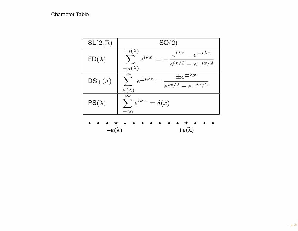
Character Table
SL(2, R) SO(2)
FD(λ)
+κ(λ)∑
−κ(λ)
eikx = − eiλx − e−iλx
eix/2 − e−ix/2
DS±(λ)
∞∑
κ(λ)
e±ikx =±e±λx
eix/2 − e−ix/2
PS(λ)
∞∑
−∞
eikx = δ(x)
−κ(λ) +κ(λ)
– p. 2/18
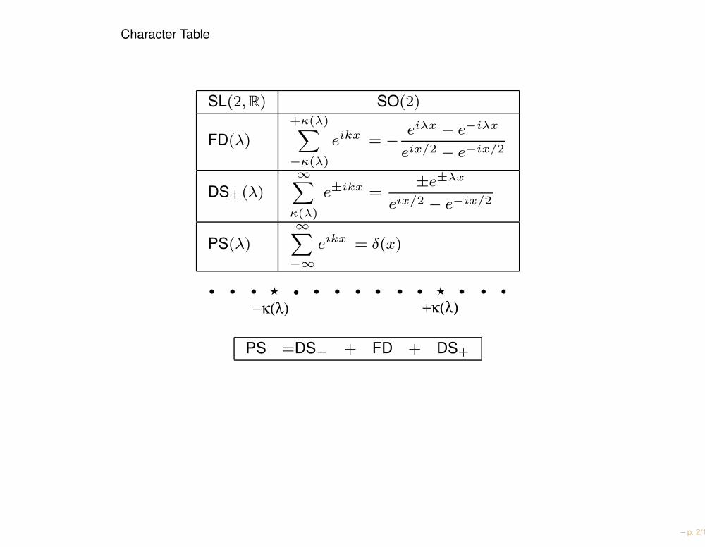
Character Table
SL(2, R) SO(2)
FD(λ)
+κ(λ)∑
−κ(λ)
eikx = − eiλx − e−iλx
eix/2 − e−ix/2
DS±(λ)
∞∑
κ(λ)
e±ikx =±e±λx
eix/2 − e−ix/2
PS(λ)
∞∑
−∞
eikx = δ(x)
−κ(λ) +κ(λ)
PS =DS− + FD + DS+
– p. 2/18
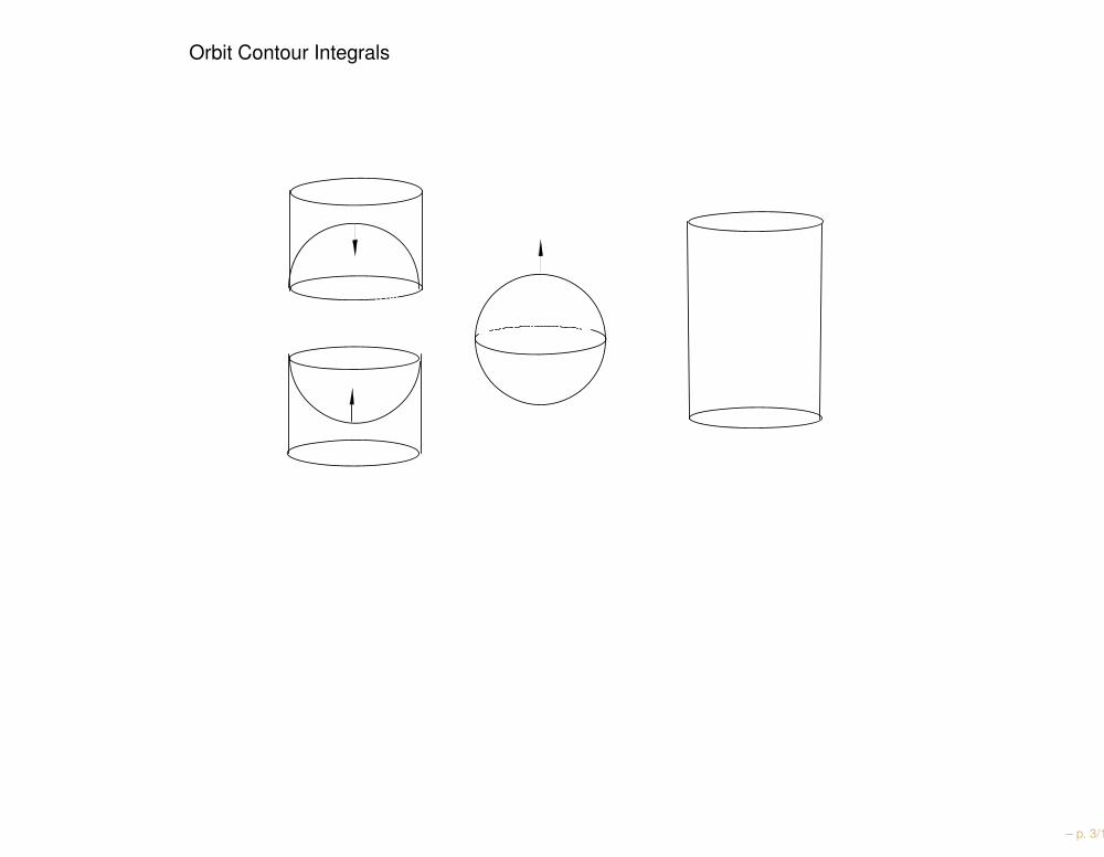
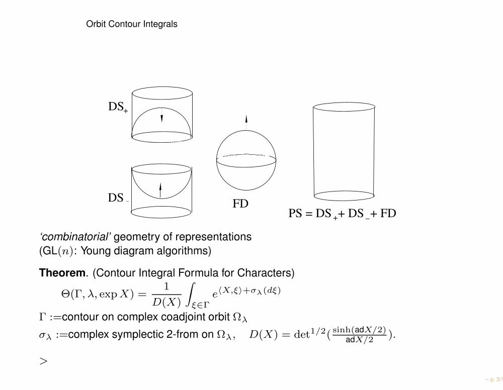
Orbit Contour Integrals
0.69
0.69
0.69
– p. 3/18
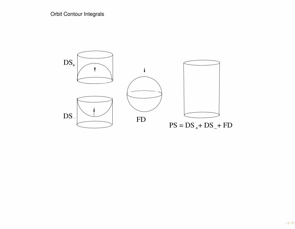
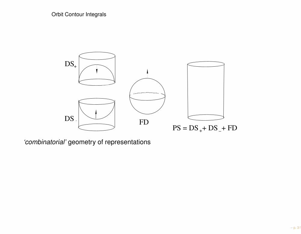
Orbit Contour Integrals
DS _
DS +
FD
0.69
0.69
0.69
PS = DS + DS + FD + _
– p. 3/18
Orbit Contour Integrals
DS _
DS +
FD
0.69
0.69
0.69
PS = DS + DS + FD + _
‘combinatorial’ geometry of representations
– p. 3/18
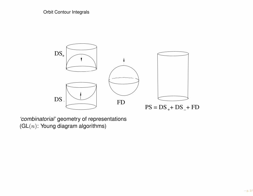
Orbit Contour Integrals
DS _
DS +
FD
0.69
0.69
0.69
PS = DS + DS + FD + _
‘combinatorial’ geometry of representations(GL(n): Young diagram algorithms)
– p. 3/18
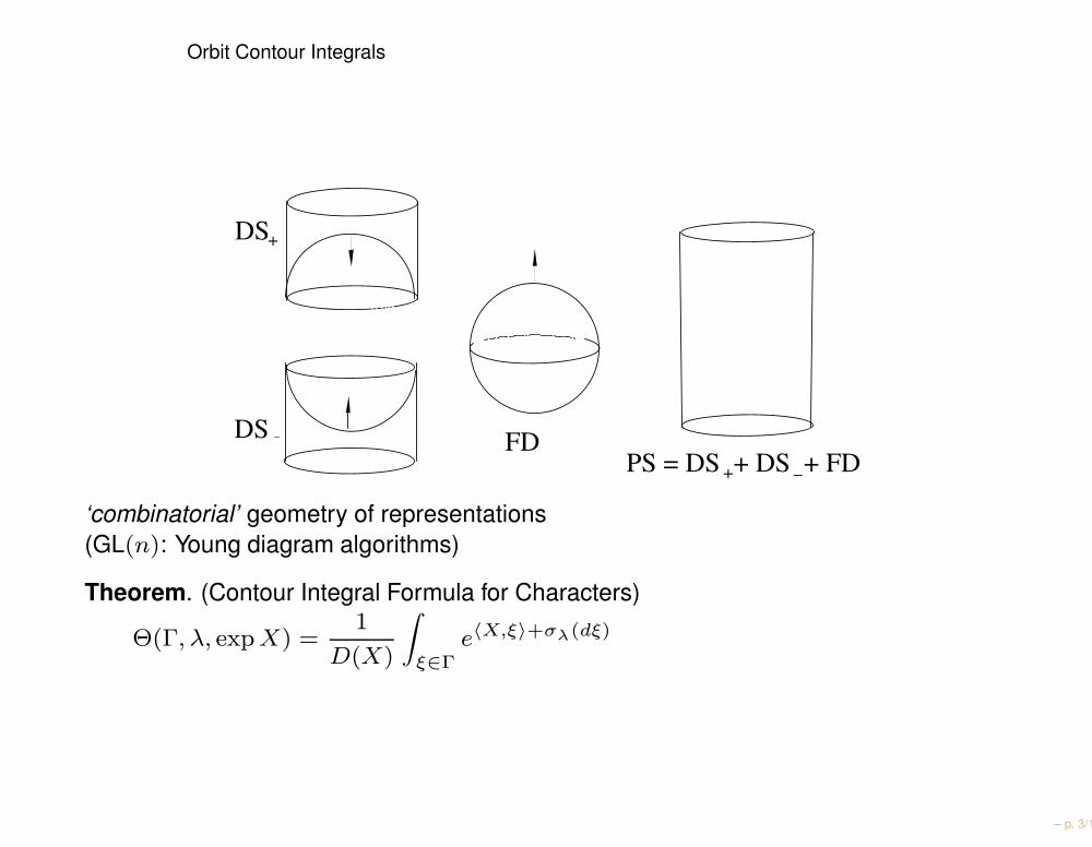
Orbit Contour Integrals
DS _
DS +
FD
0.69
0.69
0.69
PS = DS + DS + FD + _
‘combinatorial’ geometry of representations(GL(n): Young diagram algorithms)
Theorem. (Contour Integral Formula for Characters)
Θ(Γ, λ, exp X) =1
D(X)
∫
ξ∈Γe〈X,ξ〉+σλ(dξ)
– p. 3/18
Orbit Contour Integrals
DS _
DS +
FD
0.69
0.69
0.69
PS = DS + DS + FD + _
‘combinatorial’ geometry of representations(GL(n): Young diagram algorithms)
Theorem. (Contour Integral Formula for Characters)
Θ(Γ, λ, exp X) =1
D(X)
∫
ξ∈Γe〈X,ξ〉+σλ(dξ)
Γ :=contour on complex coadjoint orbit Ωλ
σλ :=complex symplectic 2-from on Ωλ, D(X) = det1/2(sinh(adX/2)
adX/2).
>
– p. 3/18

Wave Front Sets
The wave front set of a representation
– p. 4/18
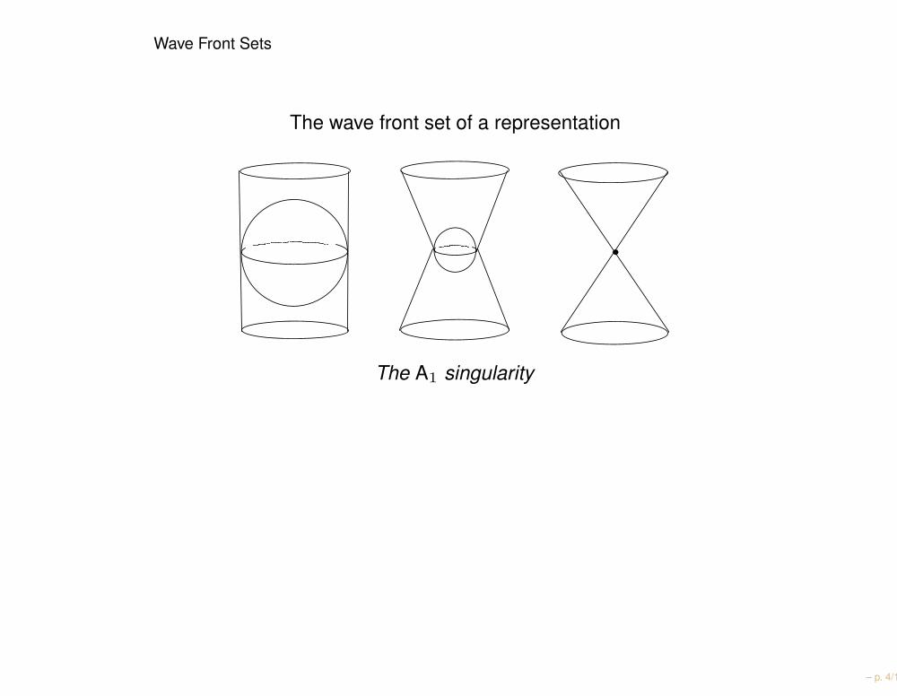
Wave Front Sets
The wave front set of a representation
The A1 singularity
– p. 4/18
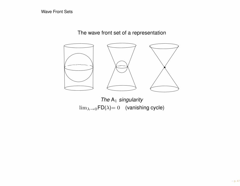
Wave Front Sets
The wave front set of a representation
The A1 singularitylimλ→0FD(λ)= 0 (vanishing cycle)
– p. 4/18
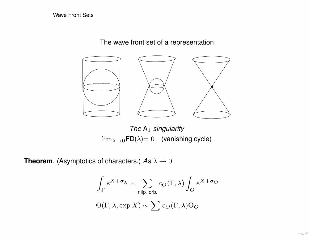
Wave Front Sets
The wave front set of a representation
The A1 singularitylimλ→0FD(λ)= 0 (vanishing cycle)
Theorem. (Asymptotics of characters.) As λ → 0
∫
ΓeX+σλ ∼
∑
nilp. orb.
cO(Γ, λ)
∫
OeX+σO
Θ(Γ, λ, exp X) ∼∑
cO(Γ, λ)ΘO
– p. 4/18
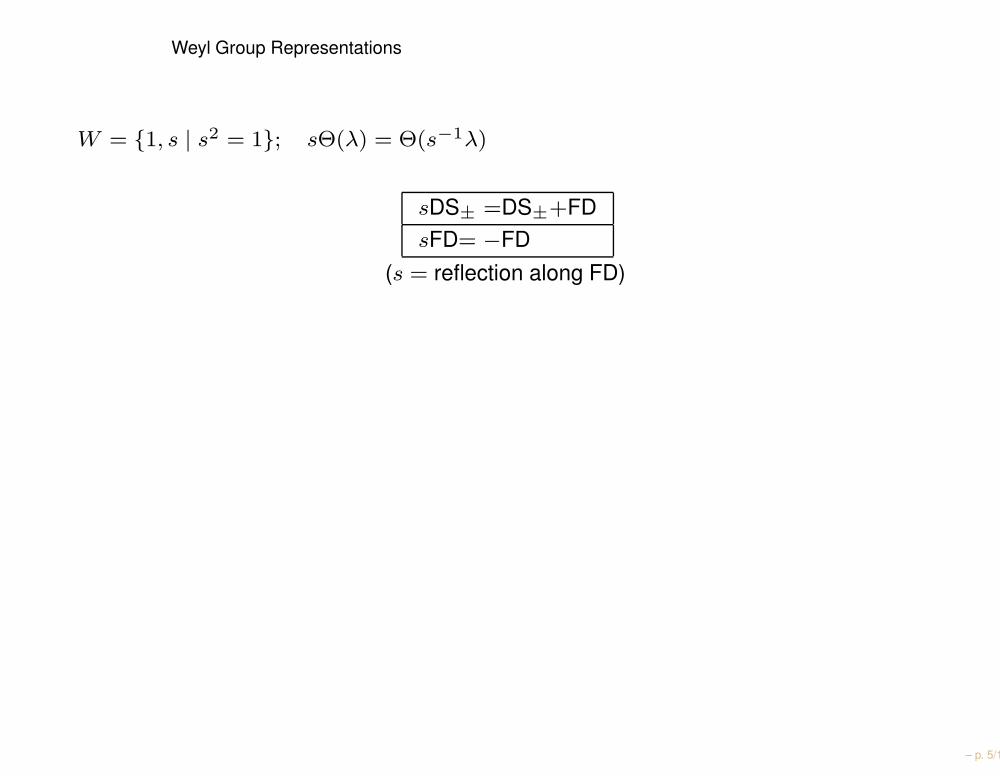
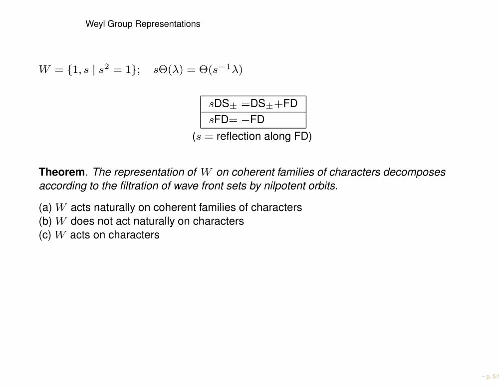
Weyl Group Representations
W = 1, s | s2 = 1; sΘ(λ) = Θ(s−1λ)
sDS± =DS±+FDsFD= −FD
(s = reflection along FD)
– p. 5/18
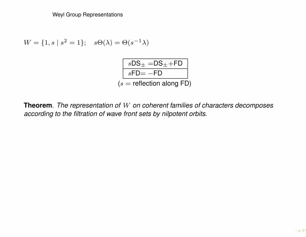
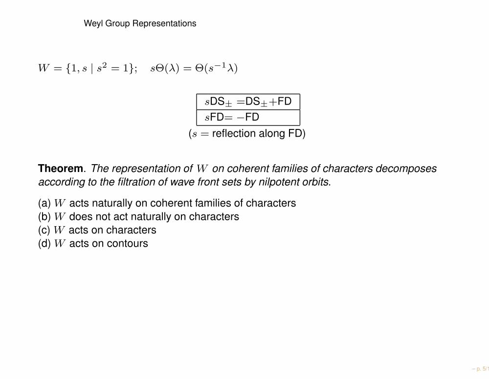
Weyl Group Representations
W = 1, s | s2 = 1; sΘ(λ) = Θ(s−1λ)
sDS± =DS±+FDsFD= −FD
(s = reflection along FD)
Theorem. The representation of W on coherent families of characters decomposesaccording to the filtration of wave front sets by nilpotent orbits.
– p. 5/18
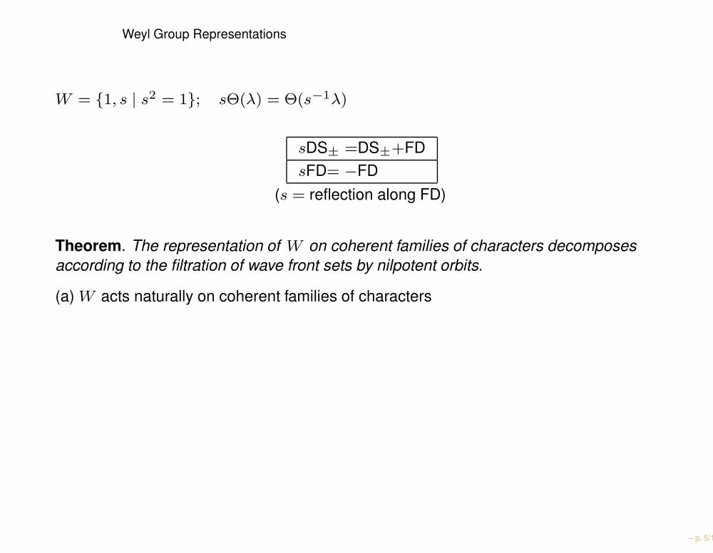
Weyl Group Representations
W = 1, s | s2 = 1; sΘ(λ) = Θ(s−1λ)
sDS± =DS±+FDsFD= −FD
(s = reflection along FD)
Theorem. The representation of W on coherent families of characters decomposesaccording to the filtration of wave front sets by nilpotent orbits.
(a) W acts naturally on coherent families of characters
– p. 5/18
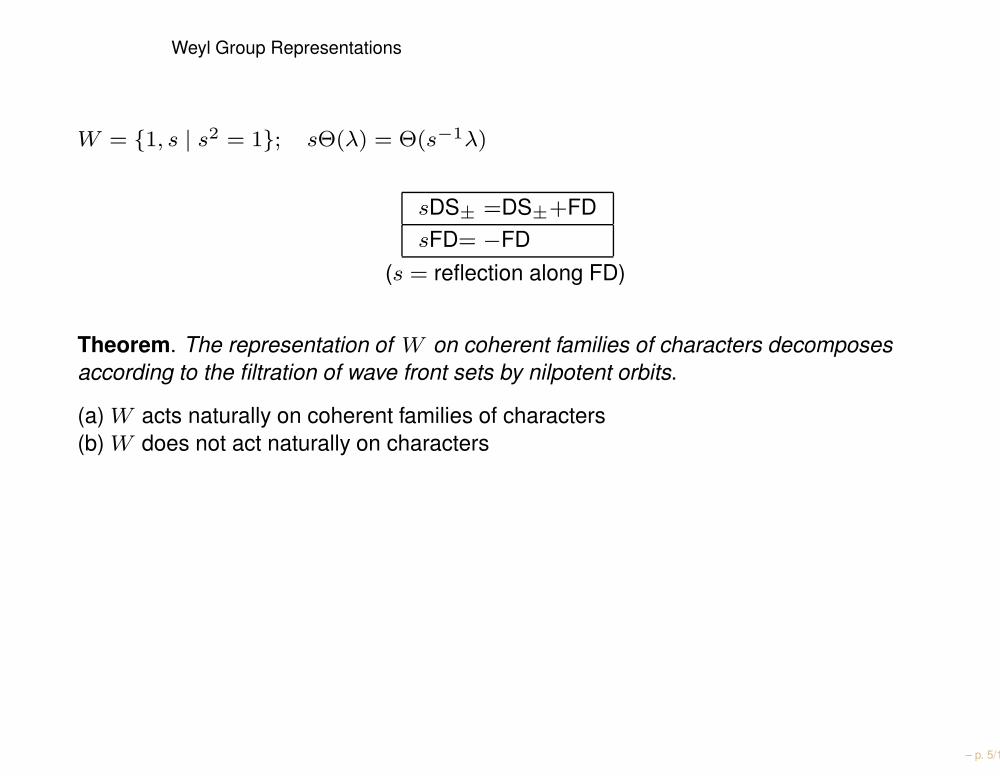
Weyl Group Representations
W = 1, s | s2 = 1; sΘ(λ) = Θ(s−1λ)
sDS± =DS±+FDsFD= −FD
(s = reflection along FD)
Theorem. The representation of W on coherent families of characters decomposesaccording to the filtration of wave front sets by nilpotent orbits.
(a) W acts naturally on coherent families of characters(b) W does not act naturally on characters
– p. 5/18
Weyl Group Representations
W = 1, s | s2 = 1; sΘ(λ) = Θ(s−1λ)
sDS± =DS±+FDsFD= −FD
(s = reflection along FD)
Theorem. The representation of W on coherent families of characters decomposesaccording to the filtration of wave front sets by nilpotent orbits.
(a) W acts naturally on coherent families of characters(b) W does not act naturally on characters(c) W acts on characters
– p. 5/18
Weyl Group Representations
W = 1, s | s2 = 1; sΘ(λ) = Θ(s−1λ)
sDS± =DS±+FDsFD= −FD
(s = reflection along FD)
Theorem. The representation of W on coherent families of characters decomposesaccording to the filtration of wave front sets by nilpotent orbits.
(a) W acts naturally on coherent families of characters(b) W does not act naturally on characters(c) W acts on characters(d) W acts on contours
– p. 5/18
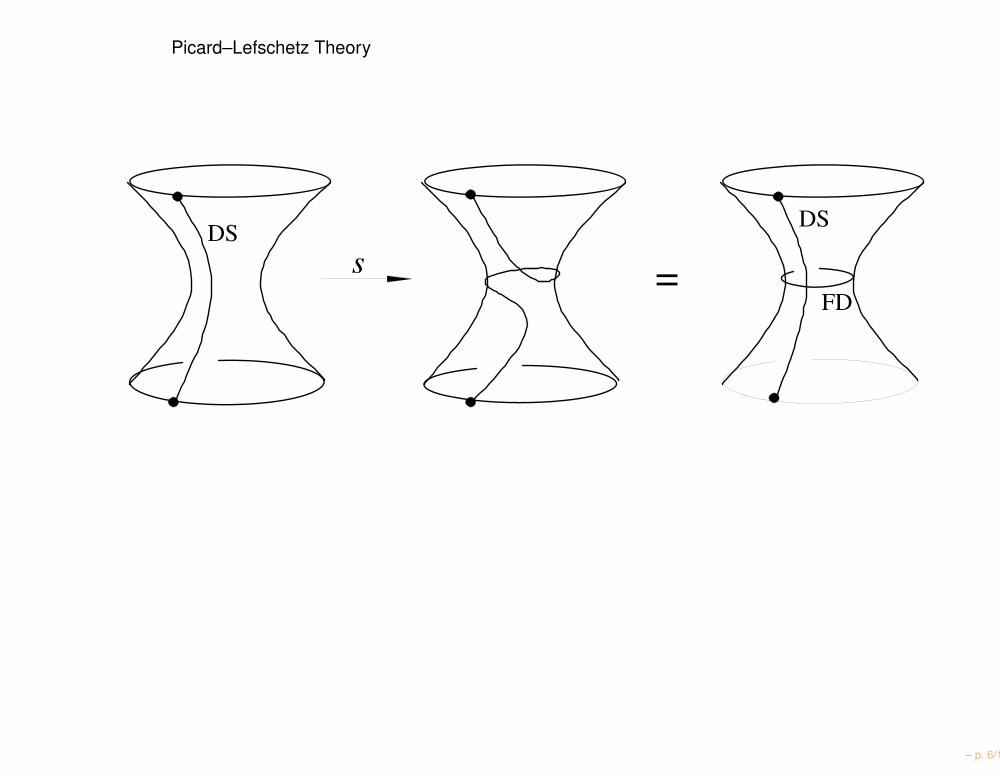
Picard–Lefschetz Theory
1.81 = DS DS
FD
s
– p. 6/18
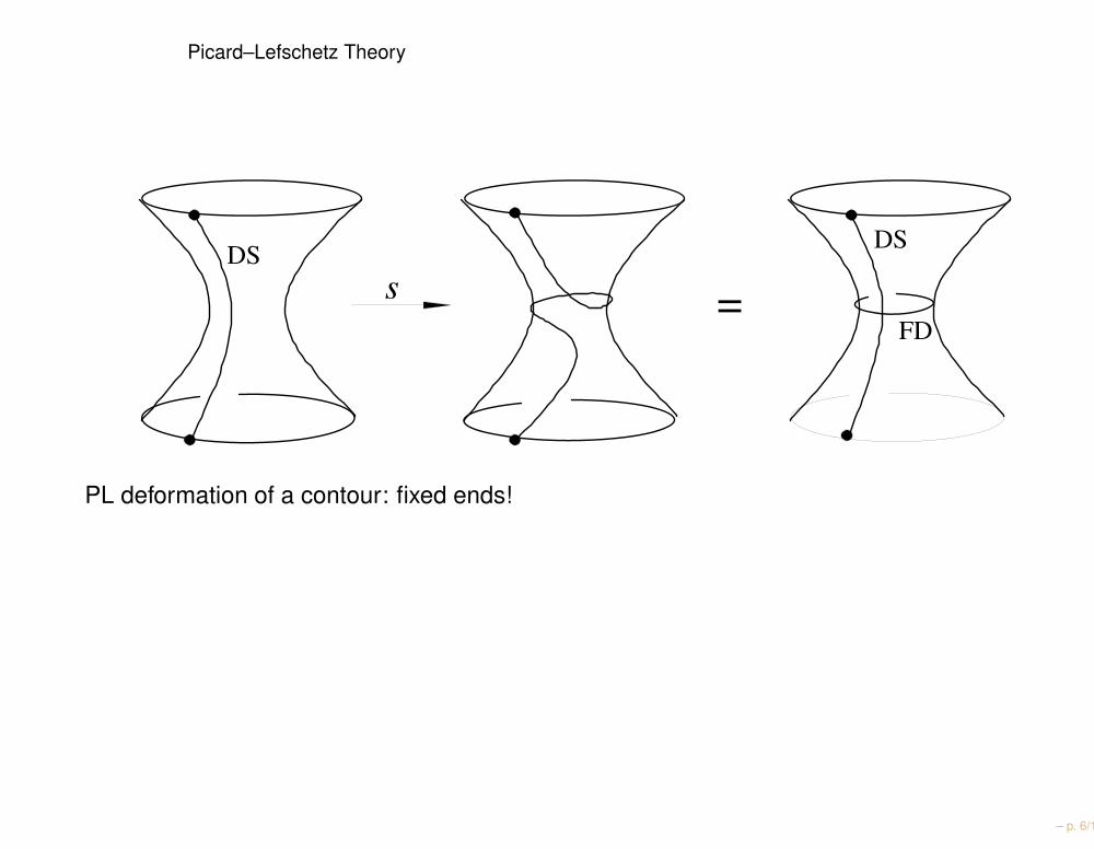
Picard–Lefschetz Theory
1.81 = DS DS
FD
s
PL deformation of a contour: fixed ends!
– p. 6/18
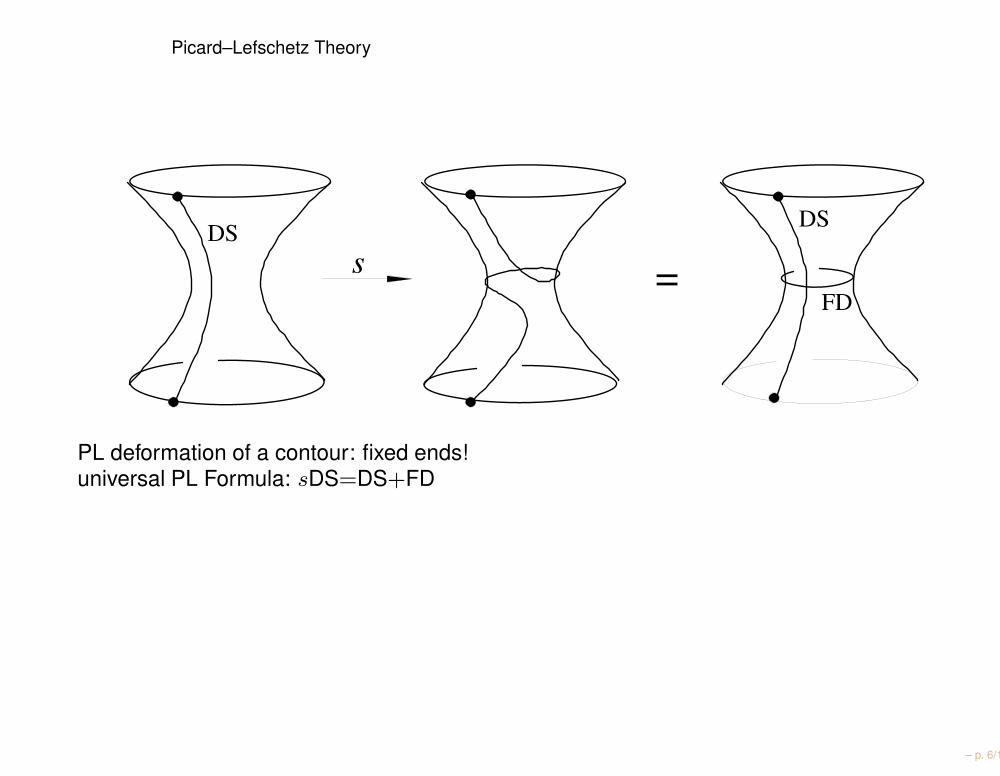
Picard–Lefschetz Theory
1.81 = DS DS
FD
s
PL deformation of a contour: fixed ends!universal PL Formula: sDS=DS+FD
– p. 6/18
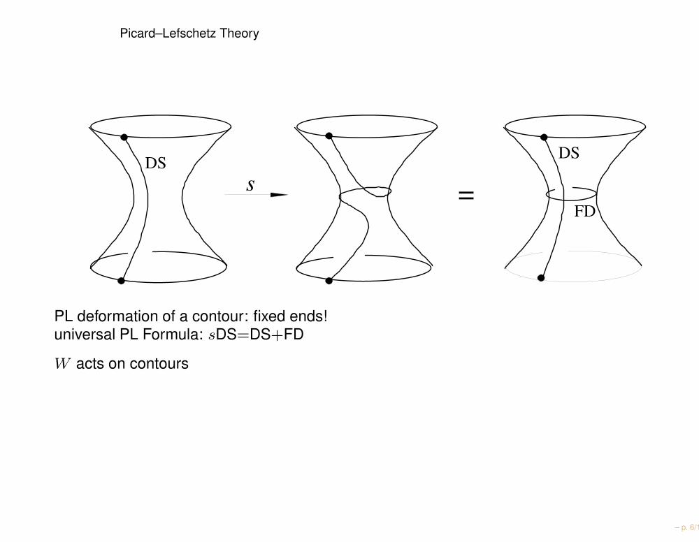
Picard–Lefschetz Theory
1.81 = DS DS
FD
s
PL deformation of a contour: fixed ends!universal PL Formula: sDS=DS+FD
W acts on contours
– p. 6/18
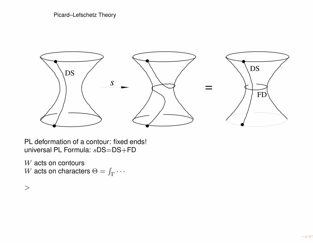
Picard–Lefschetz Theory
1.81 = DS DS
FD
s
PL deformation of a contour: fixed ends!universal PL Formula: sDS=DS+FD
W acts on contoursW acts on characters Θ =
∫
Γ · · ·
>
– p. 6/18
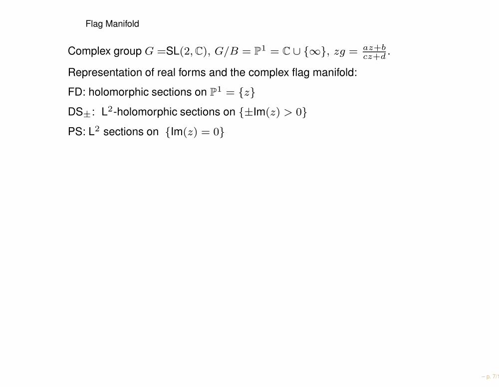
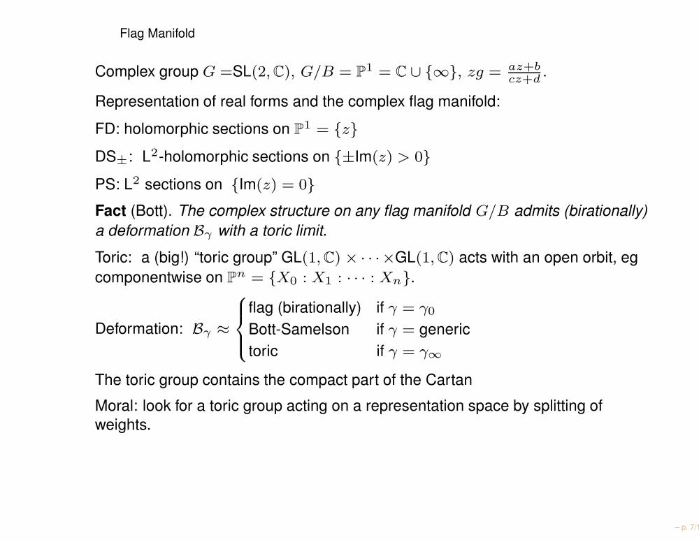
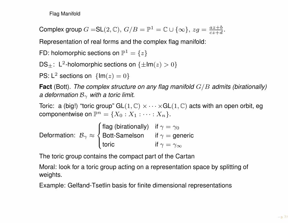
Flag Manifold
Complex group G =SL(2, C), G/B = P1 = C ∪ ∞, zg = az+bcz+d
.
Representation of real forms and the complex flag manifold:
FD: holomorphic sections on P1 = zDS±: L2-holomorphic sections on ±Im(z) > 0PS: L2 sections on Im(z) = 0Fact (Bott). The complex structure on any flag manifold G/B admits (birationally)a deformation Bγ with a toric limit.
Toric: a (big!) “toric group” GL(1, C) × · · ·×GL(1, C) acts with an open orbit, egcomponentwise on Pn = X0 : X1 : · · · : Xn.
Deformation: Bγ ≈
flag (birationally) if γ = γ0
Bott-Samelson if γ = generictoric if γ = γ∞
The toric group contains the compact part of the Cartan
Moral: look for a toric group acting on a representation space by splitting ofweights.
Example: Gelfand-Tsetlin basis for finite dimensional representations
– p. 7/18
Flag Manifold
Complex group G =SL(2, C), G/B = P1 = C ∪ ∞, zg = az+bcz+d
.
Representation of real forms and the complex flag manifold:
FD: holomorphic sections on P1 = z
DS±: L2-holomorphic sections on ±Im(z) > 0PS: L2 sections on Im(z) = 0Fact (Bott). The complex structure on any flag manifold G/B admits (birationally)a deformation Bγ with a toric limit.
Toric: a (big!) “toric group” GL(1, C) × · · ·×GL(1, C) acts with an open orbit, egcomponentwise on Pn = X0 : X1 : · · · : Xn.
Deformation: Bγ ≈
flag (birationally) if γ = γ0
Bott-Samelson if γ = generictoric if γ = γ∞
The toric group contains the compact part of the Cartan
Moral: look for a toric group acting on a representation space by splitting ofweights.
Example: Gelfand-Tsetlin basis for finite dimensional representations
– p. 7/18
Flag Manifold
Complex group G =SL(2, C), G/B = P1 = C ∪ ∞, zg = az+bcz+d
.
Representation of real forms and the complex flag manifold:
FD: holomorphic sections on P1 = zDS±: L2-holomorphic sections on ±Im(z) > 0
PS: L2 sections on Im(z) = 0Fact (Bott). The complex structure on any flag manifold G/B admits (birationally)a deformation Bγ with a toric limit.
Toric: a (big!) “toric group” GL(1, C) × · · ·×GL(1, C) acts with an open orbit, egcomponentwise on Pn = X0 : X1 : · · · : Xn.
Deformation: Bγ ≈
flag (birationally) if γ = γ0
Bott-Samelson if γ = generictoric if γ = γ∞
The toric group contains the compact part of the Cartan
Moral: look for a toric group acting on a representation space by splitting ofweights.
Example: Gelfand-Tsetlin basis for finite dimensional representations
– p. 7/18
Flag Manifold
Complex group G =SL(2, C), G/B = P1 = C ∪ ∞, zg = az+bcz+d
.
Representation of real forms and the complex flag manifold:
FD: holomorphic sections on P1 = zDS±: L2-holomorphic sections on ±Im(z) > 0PS: L2 sections on Im(z) = 0
Fact (Bott). The complex structure on any flag manifold G/B admits (birationally)a deformation Bγ with a toric limit.
Toric: a (big!) “toric group” GL(1, C) × · · ·×GL(1, C) acts with an open orbit, egcomponentwise on Pn = X0 : X1 : · · · : Xn.
Deformation: Bγ ≈
flag (birationally) if γ = γ0
Bott-Samelson if γ = generictoric if γ = γ∞
The toric group contains the compact part of the Cartan
Moral: look for a toric group acting on a representation space by splitting ofweights.
Example: Gelfand-Tsetlin basis for finite dimensional representations
– p. 7/18
Flag Manifold
Complex group G =SL(2, C), G/B = P1 = C ∪ ∞, zg = az+bcz+d
.
Representation of real forms and the complex flag manifold:
FD: holomorphic sections on P1 = zDS±: L2-holomorphic sections on ±Im(z) > 0PS: L2 sections on Im(z) = 0Fact (Bott). The complex structure on any flag manifold G/B admits (birationally)a deformation Bγ with a toric limit.
Toric: a (big!) “toric group” GL(1, C) × · · ·×GL(1, C) acts with an open orbit, egcomponentwise on Pn = X0 : X1 : · · · : Xn.
Deformation: Bγ ≈
flag (birationally) if γ = γ0
Bott-Samelson if γ = generictoric if γ = γ∞
The toric group contains the compact part of the Cartan
Moral: look for a toric group acting on a representation space by splitting ofweights.
Example: Gelfand-Tsetlin basis for finite dimensional representations
– p. 7/18
Flag Manifold
Complex group G =SL(2, C), G/B = P1 = C ∪ ∞, zg = az+bcz+d
.
Representation of real forms and the complex flag manifold:
FD: holomorphic sections on P1 = zDS±: L2-holomorphic sections on ±Im(z) > 0PS: L2 sections on Im(z) = 0Fact (Bott). The complex structure on any flag manifold G/B admits (birationally)a deformation Bγ with a toric limit.
Toric: a (big!) “toric group” GL(1, C) × · · ·×GL(1, C) acts with an open orbit, egcomponentwise on Pn = X0 : X1 : · · · : Xn.
Deformation: Bγ ≈
flag (birationally) if γ = γ0
Bott-Samelson if γ = generictoric if γ = γ∞
The toric group contains the compact part of the Cartan
Moral: look for a toric group acting on a representation space by splitting ofweights.
Example: Gelfand-Tsetlin basis for finite dimensional representations
– p. 7/18
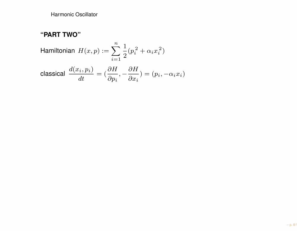
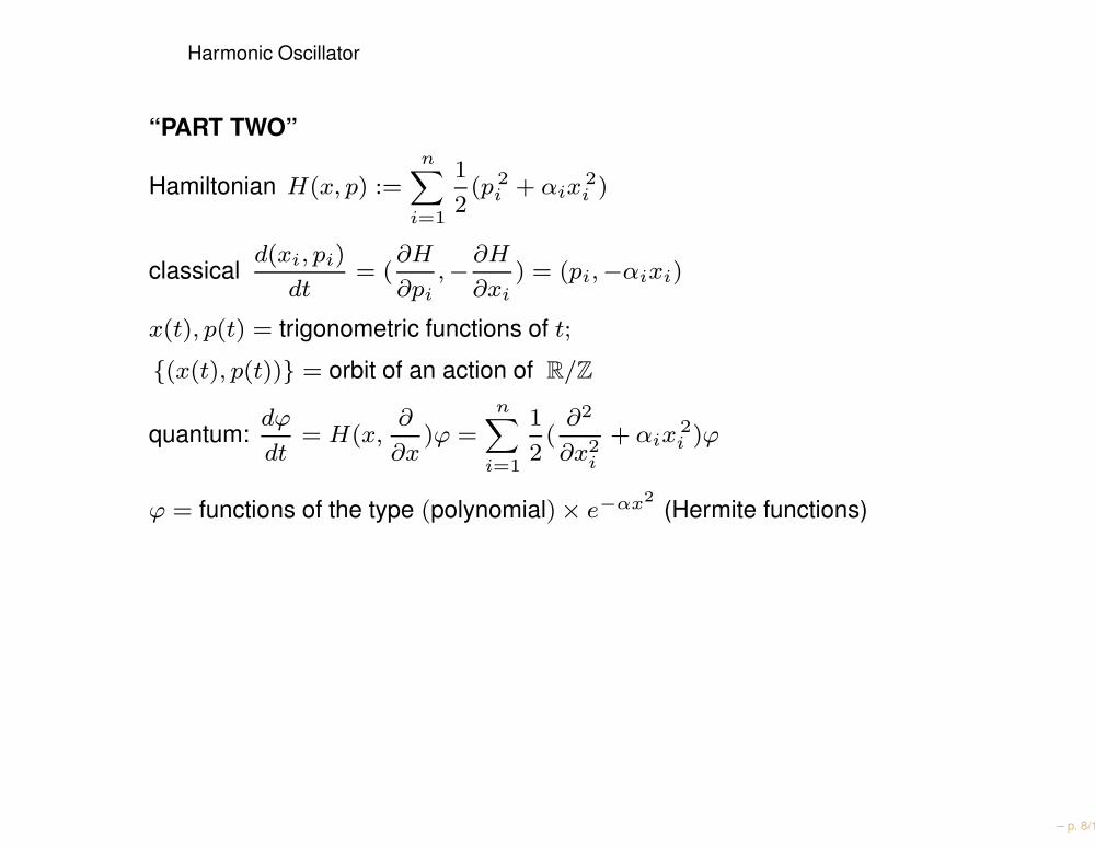
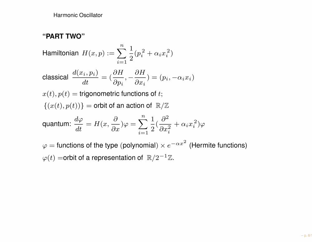
Harmonic Oscillator
“PART TWO”
Hamiltonian H(x, p) :=n
∑
i=1
1
2(p 2
i + αix2i )
classicald(xi, pi)
dt= (
∂H
∂pi,− ∂H
∂xi) = (pi,−αixi)
x(t), p(t) = trigonometric functions of t;
(x(t), p(t)) = orbit of an action of R/Z
quantum:dϕ
dt= H(x,
∂
∂x)ϕ =
n∑
i=1
1
2(
∂2
∂x2i
+ αix2i )ϕ
ϕ = functions of the type (polynomial)× e−αx2
(Hermite functions)
ϕ(t) =orbit of a representation of R/2−1Z.
– p. 8/18
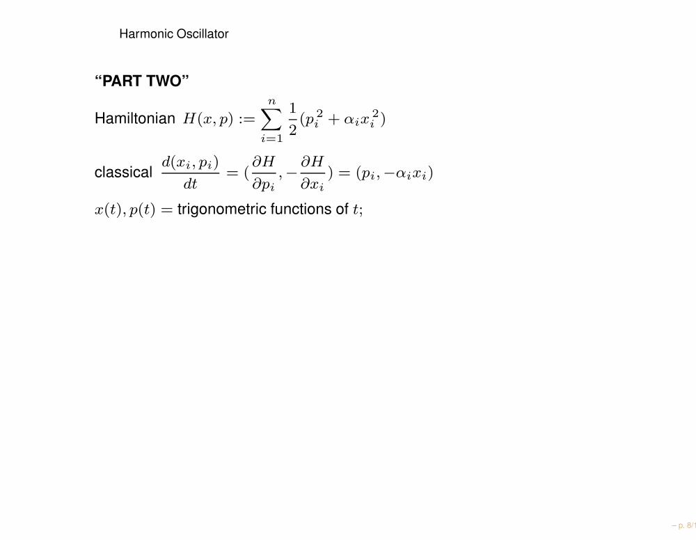
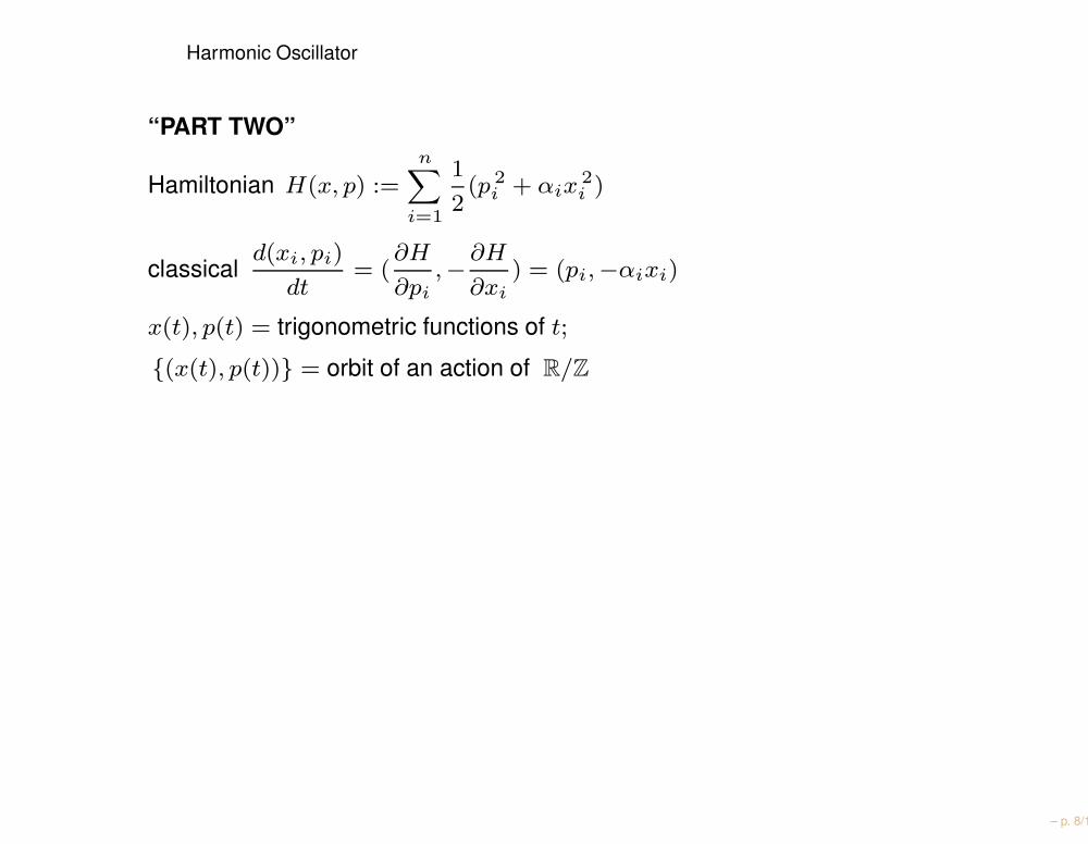
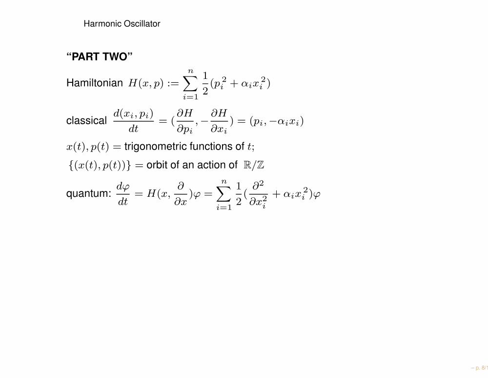
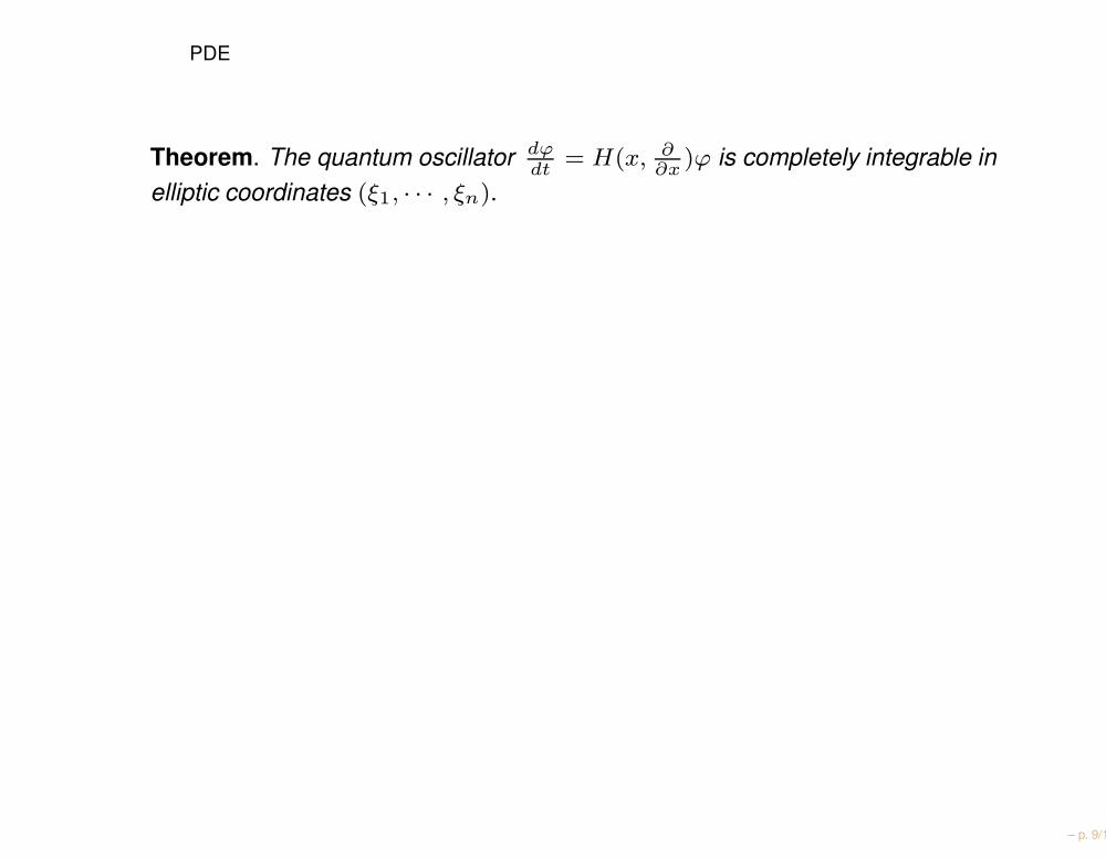
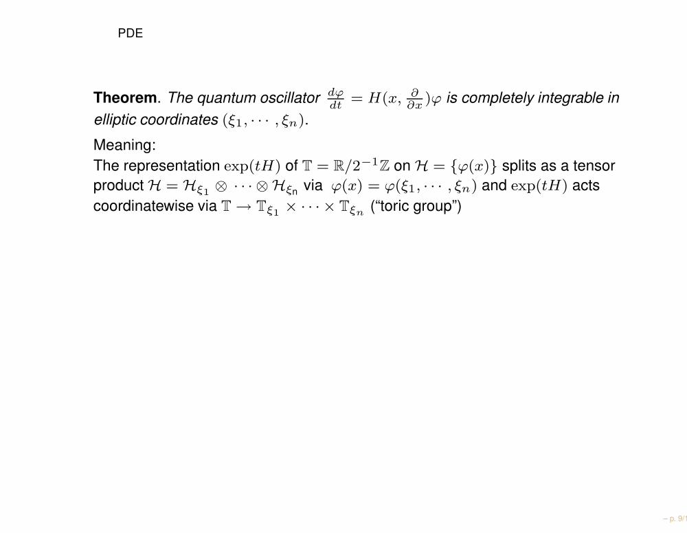
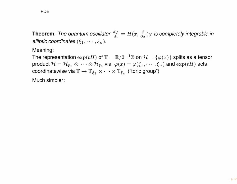
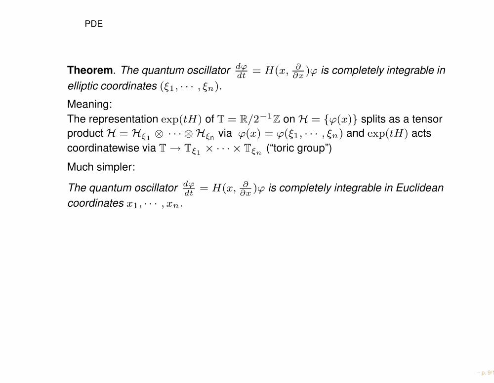
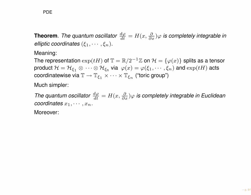
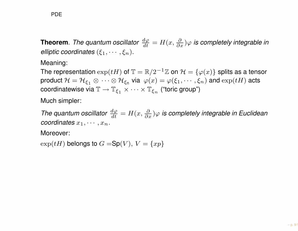
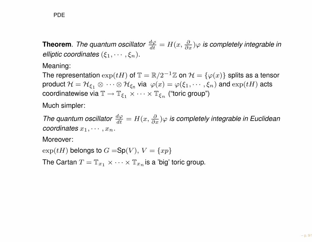
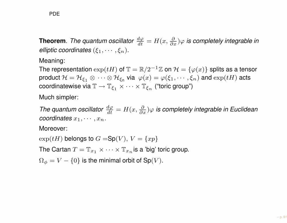
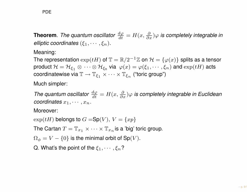
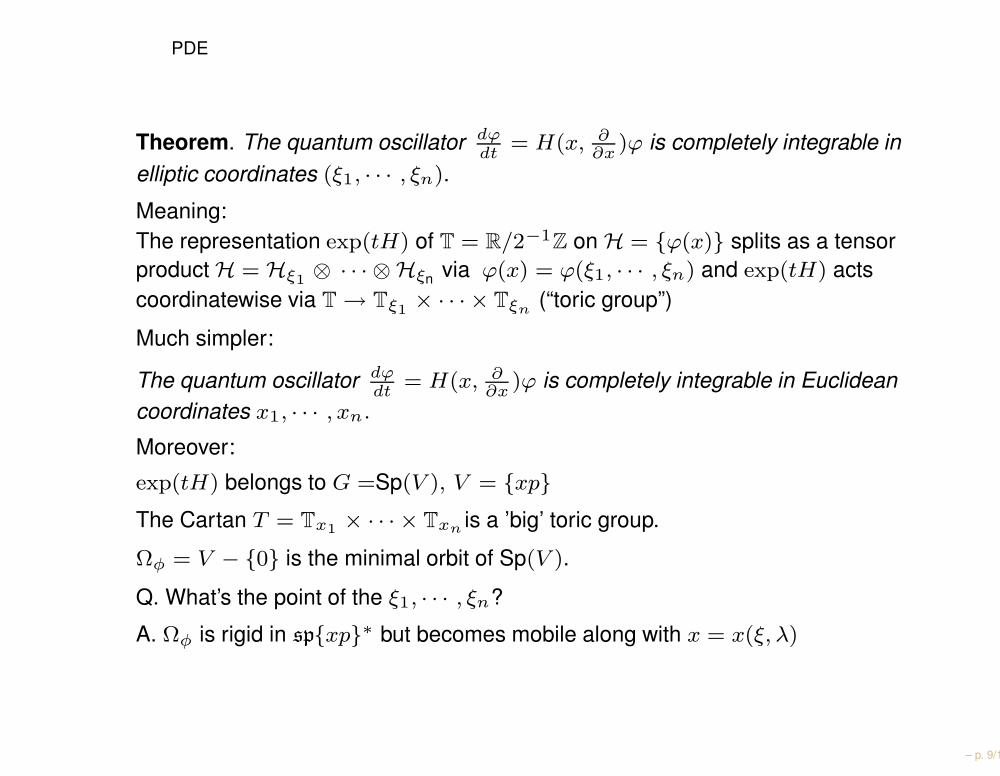
PDE
Theorem. The quantum oscillator dϕdt
= H(x, ∂∂x
)ϕ is completely integrable inelliptic coordinates (ξ1, · · · , ξn).
Meaning:The representation exp(tH) of T = R/2−1Z on H = ϕ(x) splits as a tensorproduct H = Hξ1 ⊗ · · · ⊗ Hξn via ϕ(x) = ϕ(ξ1, · · · , ξn) and exp(tH) actscoordinatewise via T → Tξ1 × · · · × Tξn
(“toric group”)
Much simpler:
The quantum oscillator dϕdt
= H(x, ∂∂x
)ϕ is completely integrable in Euclideancoordinates x1, · · · , xn.
Moreover:
exp(tH) belongs to G =Sp(V ), V = xpThe Cartan T = Tx1
× · · · × Txnis a ’big’ toric group.
Ωφ = V − 0 is the minimal orbit of Sp(V ).
Q. What’s the point of the ξ1, · · · , ξn?
A. Ωφ is rigid in spxp∗ but becomes mobile along with x = x(ξ, λ)
– p. 9/18
PDE
Theorem. The quantum oscillator dϕdt
= H(x, ∂∂x
)ϕ is completely integrable inelliptic coordinates (ξ1, · · · , ξn).
Meaning:The representation exp(tH) of T = R/2−1Z on H = ϕ(x) splits as a tensorproduct H = Hξ1 ⊗ · · · ⊗ Hξn via ϕ(x) = ϕ(ξ1, · · · , ξn) and exp(tH) actscoordinatewise via T → Tξ1 × · · · × Tξn
(“toric group”)
Much simpler:
The quantum oscillator dϕdt
= H(x, ∂∂x
)ϕ is completely integrable in Euclideancoordinates x1, · · · , xn.
Moreover:
exp(tH) belongs to G =Sp(V ), V = xp
The Cartan T = Tx1× · · · × Txn
is a ’big’ toric group.
Ωφ = V − 0 is the minimal orbit of Sp(V ).
Q. What’s the point of the ξ1, · · · , ξn?
A. Ωφ is rigid in spxp∗ but becomes mobile along with x = x(ξ, λ)
– p. 9/18
PDE
Theorem. The quantum oscillator dϕdt
= H(x, ∂∂x
)ϕ is completely integrable inelliptic coordinates (ξ1, · · · , ξn).
Meaning:The representation exp(tH) of T = R/2−1Z on H = ϕ(x) splits as a tensorproduct H = Hξ1 ⊗ · · · ⊗ Hξn via ϕ(x) = ϕ(ξ1, · · · , ξn) and exp(tH) actscoordinatewise via T → Tξ1 × · · · × Tξn
(“toric group”)
Much simpler:
The quantum oscillator dϕdt
= H(x, ∂∂x
)ϕ is completely integrable in Euclideancoordinates x1, · · · , xn.
Moreover:
exp(tH) belongs to G =Sp(V ), V = xpThe Cartan T = Tx1
× · · · × Txnis a ’big’ toric group.
Ωφ = V − 0 is the minimal orbit of Sp(V ).
Q. What’s the point of the ξ1, · · · , ξn?
A. Ωφ is rigid in spxp∗ but becomes mobile along with x = x(ξ, λ)
– p. 9/18
PDE
Theorem. The quantum oscillator dϕdt
= H(x, ∂∂x
)ϕ is completely integrable inelliptic coordinates (ξ1, · · · , ξn).
Meaning:The representation exp(tH) of T = R/2−1Z on H = ϕ(x) splits as a tensorproduct H = Hξ1 ⊗ · · · ⊗ Hξn via ϕ(x) = ϕ(ξ1, · · · , ξn) and exp(tH) actscoordinatewise via T → Tξ1 × · · · × Tξn
(“toric group”)
Much simpler:
The quantum oscillator dϕdt
= H(x, ∂∂x
)ϕ is completely integrable in Euclideancoordinates x1, · · · , xn.
Moreover:
exp(tH) belongs to G =Sp(V ), V = xpThe Cartan T = Tx1
× · · · × Txnis a ’big’ toric group.
Ωφ = V − 0 is the minimal orbit of Sp(V ).
Q. What’s the point of the ξ1, · · · , ξn?
A. Ωφ is rigid in spxp∗ but becomes mobile along with x = x(ξ, λ)
– p. 9/18
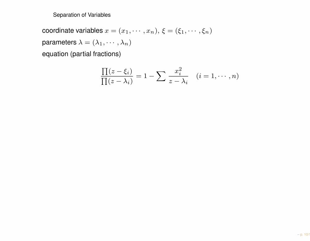
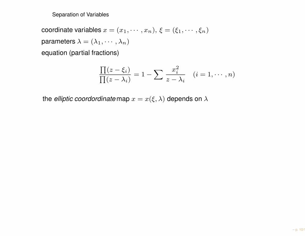
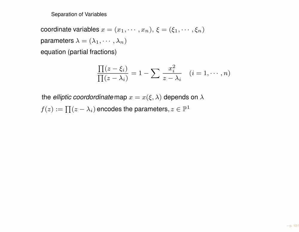
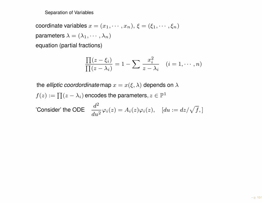
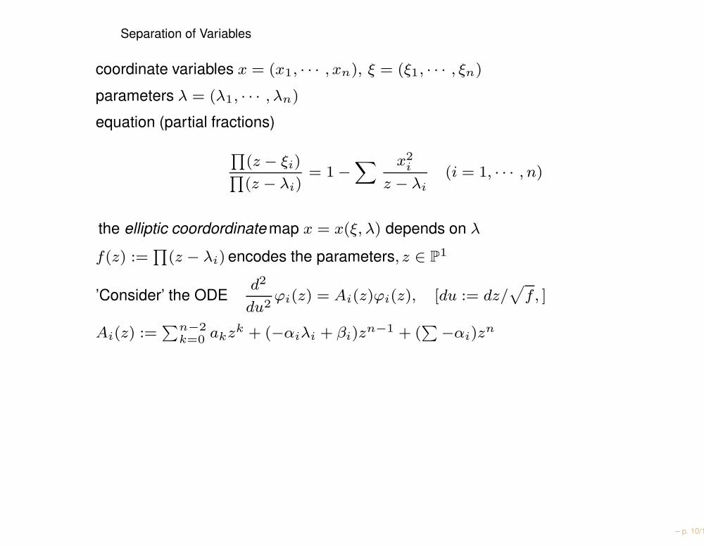
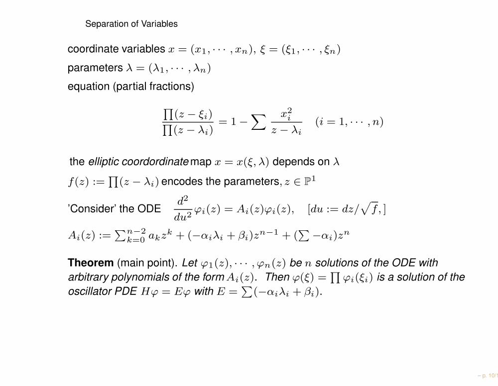
Separation of Variables
coordinate variables x = (x1, · · · , xn), ξ = (ξ1, · · · , ξn)
parameters λ = (λ1, · · · , λn)
equation (partial fractions)
∏
(z − ξi)∏
(z − λi)= 1 −
∑ x2i
z − λi(i = 1, · · · , n)
the elliptic coordordinate map x = x(ξ, λ) depends on λ
f(z) :=∏
(z − λi) encodes the parameters, z ∈ P1
’Consider’ the ODEd2
du2ϕi(z) = Ai(z)ϕi(z), [du := dz/
√
f, ]
Ai(z) :=∑n−2
k=0 akzk + (−αiλi + βi)zn−1 + (
∑
−αi)zn
Theorem (main point). Let ϕ1(z), · · · , ϕn(z) be n solutions of the ODE witharbitrary polynomials of the form Ai(z). Then ϕ(ξ) =
∏
ϕi(ξi) is a solution of theoscillator PDE Hϕ = Eϕ with E =
∑
(−αiλi + βi).
– p. 10/18
Elliptic Contour Integrals
n = 3; f(z) := (z − λ1)(z − λ2)(z − λ3)
∏
(z − ξi)∏
(z − λi)= 1 −
∑ x2i
z − λi(i = 1, · · · , 3)
solution (“generic point” ξx):
– p. 11/18

Elliptic Contour Integrals
n = 3; f(z) := (z − λ1)(z − λ2)(z − λ3)
∏
(z − ξi)∏
(z − λi)= 1 −
∑ x2i
z − λi(i = 1, · · · , 3)
solution (“generic point” ξx):
– p. 11/18
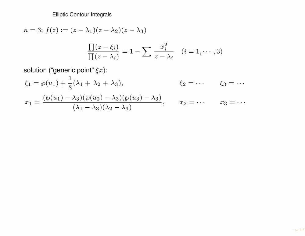
Elliptic Contour Integrals
n = 3; f(z) := (z − λ1)(z − λ2)(z − λ3)
∏
(z − ξi)∏
(z − λi)= 1 −
∑ x2i
z − λi(i = 1, · · · , 3)
solution (“generic point” ξx):
ξ1 = ℘(u1) +1
3(λ1 + λ2 + λ3), ξ2 = · · · ξ3 = · · ·
x1 =(℘(u1) − λ3)(℘(u2) − λ3)(℘(u3) − λ3)
(λ1 − λ3)(λ2 − λ3), x2 = · · · x3 = · · ·
– p. 11/18
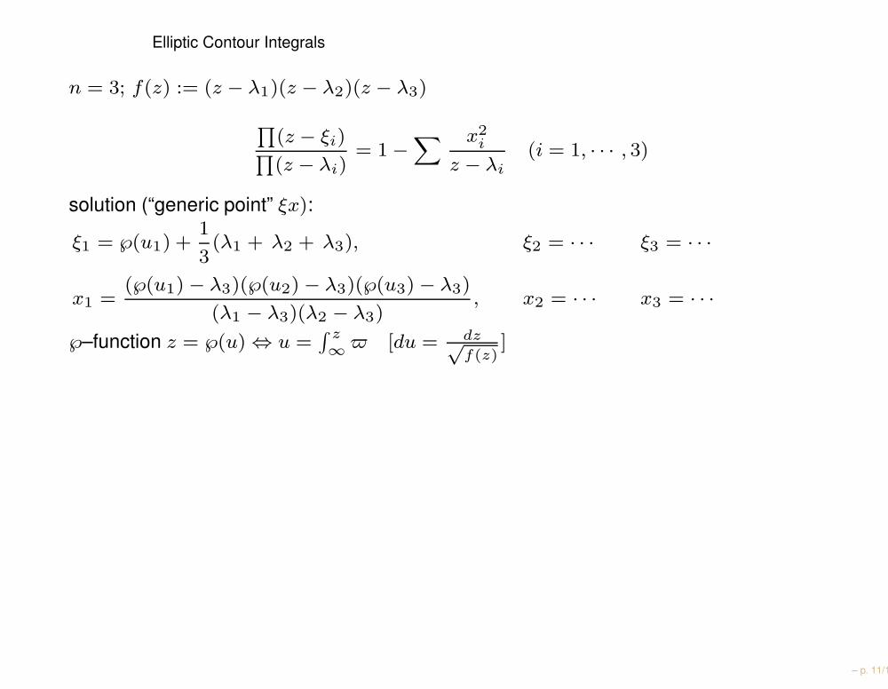
Elliptic Contour Integrals
n = 3; f(z) := (z − λ1)(z − λ2)(z − λ3)
∏
(z − ξi)∏
(z − λi)= 1 −
∑ x2i
z − λi(i = 1, · · · , 3)
solution (“generic point” ξx):
ξ1 = ℘(u1) +1
3(λ1 + λ2 + λ3), ξ2 = · · · ξ3 = · · ·
x1 =(℘(u1) − λ3)(℘(u2) − λ3)(℘(u3) − λ3)
(λ1 − λ3)(λ2 − λ3), x2 = · · · x3 = · · ·
℘–function z = ℘(u) ⇔ u =∫ z∞ $ [du = dz√
f(z)]
– p. 11/18
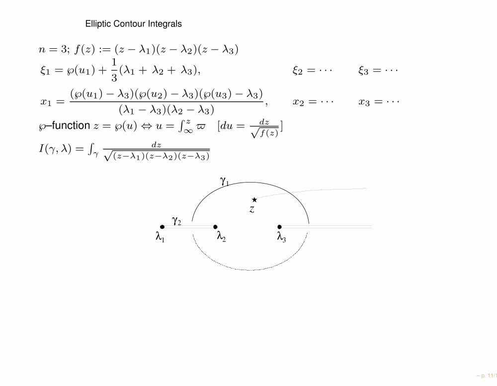
Elliptic Contour Integrals
n = 3; f(z) := (z − λ1)(z − λ2)(z − λ3)
ξ1 = ℘(u1) +1
3(λ1 + λ2 + λ3), ξ2 = · · · ξ3 = · · ·
x1 =(℘(u1) − λ3)(℘(u2) − λ3)(℘(u3) − λ3)
(λ1 − λ3)(λ2 − λ3), x2 = · · · x3 = · · ·
℘–function z = ℘(u) ⇔ u =∫ z∞ $ [du = dz√
f(z)]
I(γ, λ) =∫
γdz√
(z−λ1)(z−λ2)(z−λ3)
z
λ 3 λ 1 λ 2
γ 1
γ 2
– p. 11/18
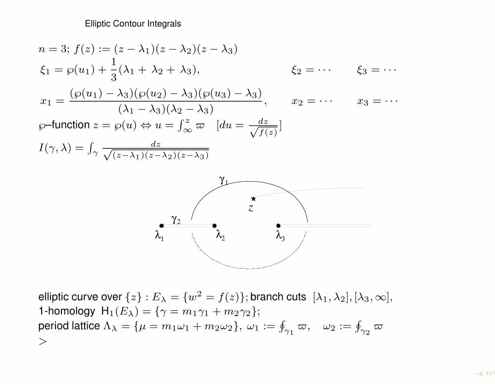
Elliptic Contour Integrals
n = 3; f(z) := (z − λ1)(z − λ2)(z − λ3)
ξ1 = ℘(u1) +1
3(λ1 + λ2 + λ3), ξ2 = · · · ξ3 = · · ·
x1 =(℘(u1) − λ3)(℘(u2) − λ3)(℘(u3) − λ3)
(λ1 − λ3)(λ2 − λ3), x2 = · · · x3 = · · ·
℘–function z = ℘(u) ⇔ u =∫ z∞ $ [du = dz√
f(z)]
I(γ, λ) =∫
γdz√
(z−λ1)(z−λ2)(z−λ3)
z
λ 3 λ 1 λ 2
γ 1
γ 2
elliptic curve over z : Eλ = w2 = f(z); branch cuts [λ1, λ2], [λ3,∞],
1-homology H1(Eλ) = γ = m1γ1 + m2γ2;period lattice Λλ = µ = m1ω1 + m2ω2, ω1 :=
∮
γ1$, ω2 :=
∮
γ2$
>
– p. 11/18

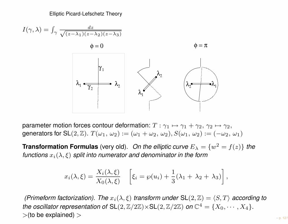
Elliptic Picard-Lefschetz Theory
I(γ, λ) =∫
γdz√
(z−λ1)(z−λ2)(z−λ3)
z
λ 3 λ 1 λ 2
γ 1
γ 2
– p. 12/18
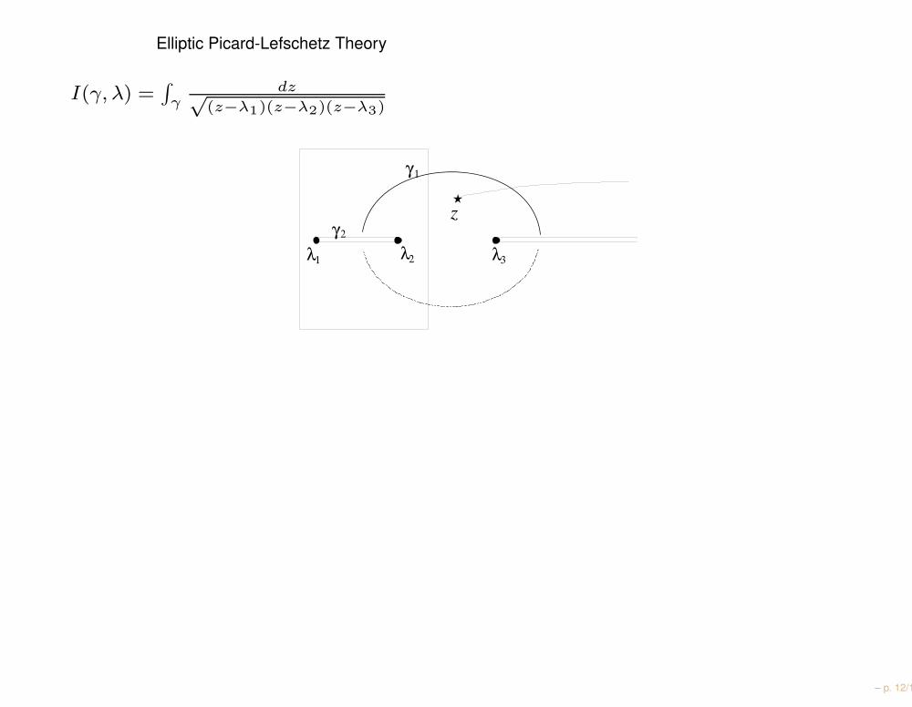
Elliptic Picard-Lefschetz Theory
I(γ, λ) =∫
γdz√
(z−λ1)(z−λ2)(z−λ3)
z
λ 3 λ 1 λ 2
γ 1
γ 2
– p. 12/18
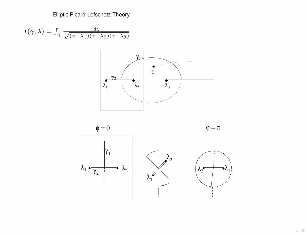
Elliptic Picard-Lefschetz Theory
I(γ, λ) =∫
γdz√
(z−λ1)(z−λ2)(z−λ3)
z
λ 3 λ 1 λ 2
γ 1
γ 2
λ 1
λ 2
λ 1 λ 2 λ 1 λ 2 γ 2
γ 1
φ = 0 φ = π
– p. 12/18
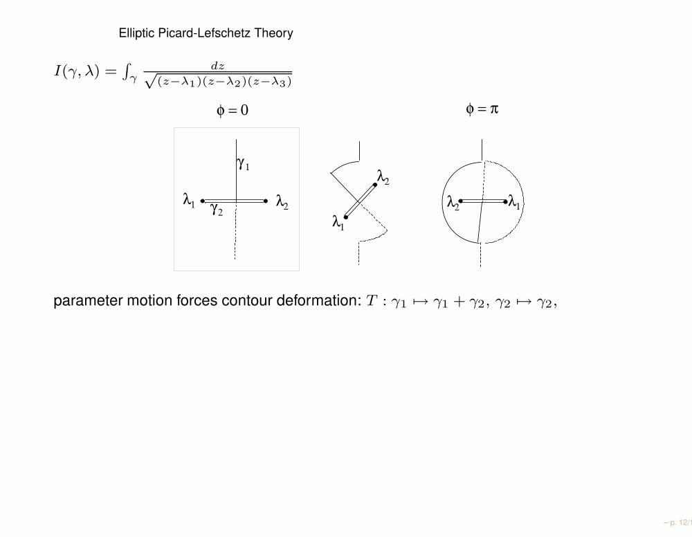
Elliptic Picard-Lefschetz Theory
I(γ, λ) =∫
γdz√
(z−λ1)(z−λ2)(z−λ3)
λ 1
λ 2
λ 1 λ 2 λ 1 λ 2 γ 2
γ 1
φ = 0 φ = π
parameter motion forces contour deformation: T : γ1 7→ γ1 + γ2, γ2 7→ γ2,
– p. 12/18
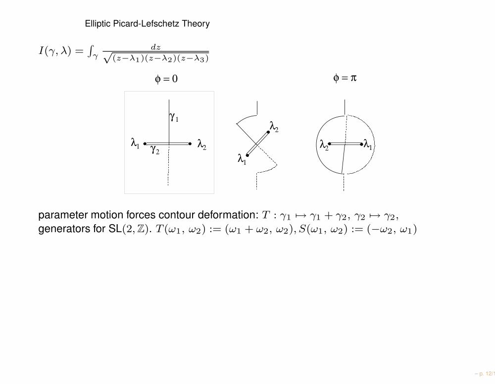
Elliptic Picard-Lefschetz Theory
I(γ, λ) =∫
γdz√
(z−λ1)(z−λ2)(z−λ3)
λ 1
λ 2
λ 1 λ 2 λ 1 λ 2 γ 2
γ 1
φ = 0 φ = π
parameter motion forces contour deformation: T : γ1 7→ γ1 + γ2, γ2 7→ γ2,
generators for SL(2, Z). T (ω1, ω2) := (ω1 + ω2, ω2), S(ω1, ω2) := (−ω2, ω1)
– p. 12/18
Elliptic Picard-Lefschetz Theory
I(γ, λ) =∫
γdz√
(z−λ1)(z−λ2)(z−λ3)
λ 1
λ 2
λ 1 λ 2 λ 1 λ 2 γ 2
γ 1
φ = 0 φ = π
parameter motion forces contour deformation: T : γ1 7→ γ1 + γ2, γ2 7→ γ2,
generators for SL(2, Z). T (ω1, ω2) := (ω1 + ω2, ω2), S(ω1, ω2) := (−ω2, ω1)
Transformation Formulas (very old). On the elliptic curve Eλ = w2 = f(z) thefunctions xi(λ, ξ) split into numerator and denominator in the form
xi(λ, ξ) =Xi(λ, ξ)
X0(λ, ξ)
[
ξi = ℘(ui) +1
3(λ1 + λ2 + λ3)
]
,
(Primeform factorization). The xi(λ, ξ) transform under SL(2, Z) = 〈S, T 〉 according tothe oscillator representation of SL(2, Z/2Z)×SL(2, Z/2Z) on C4 = X0, · · · , X4.>(to be explained) >
– p. 12/18
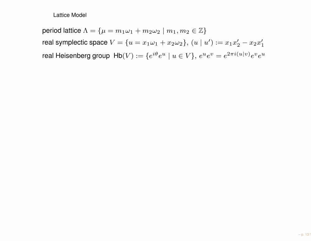
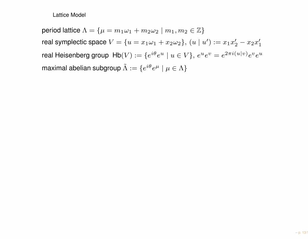
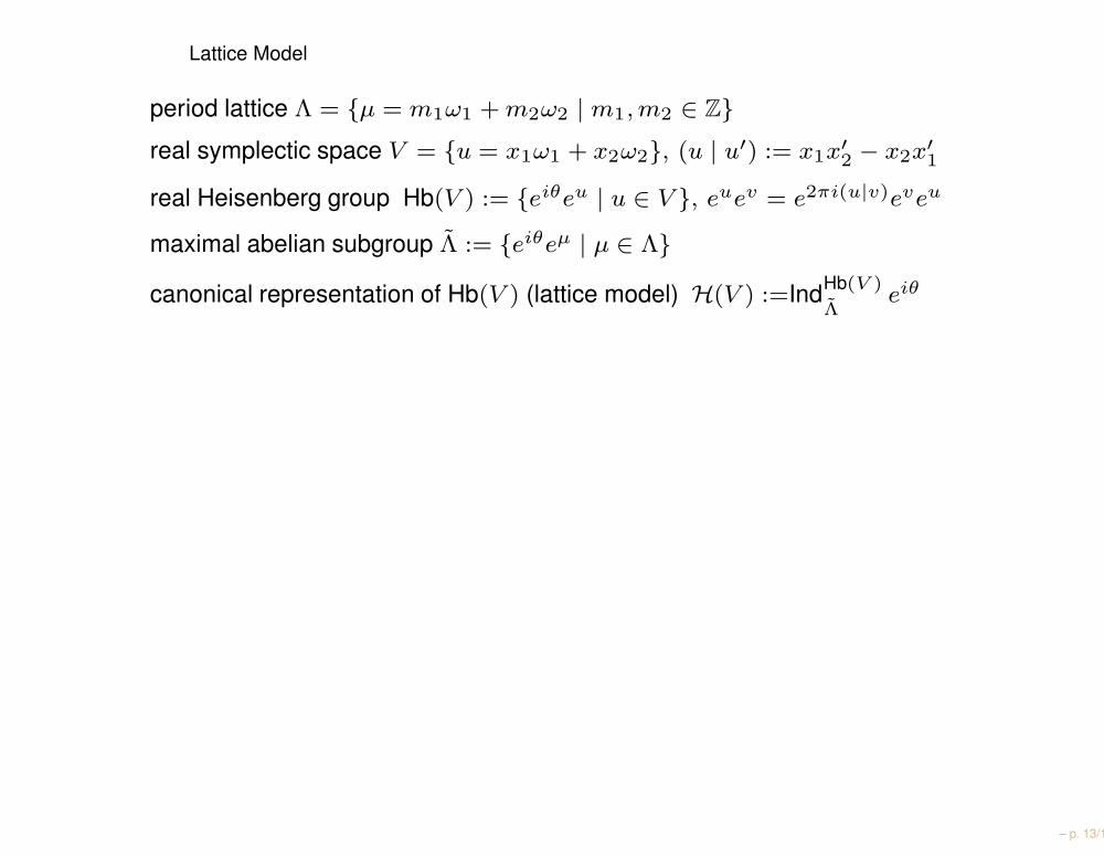
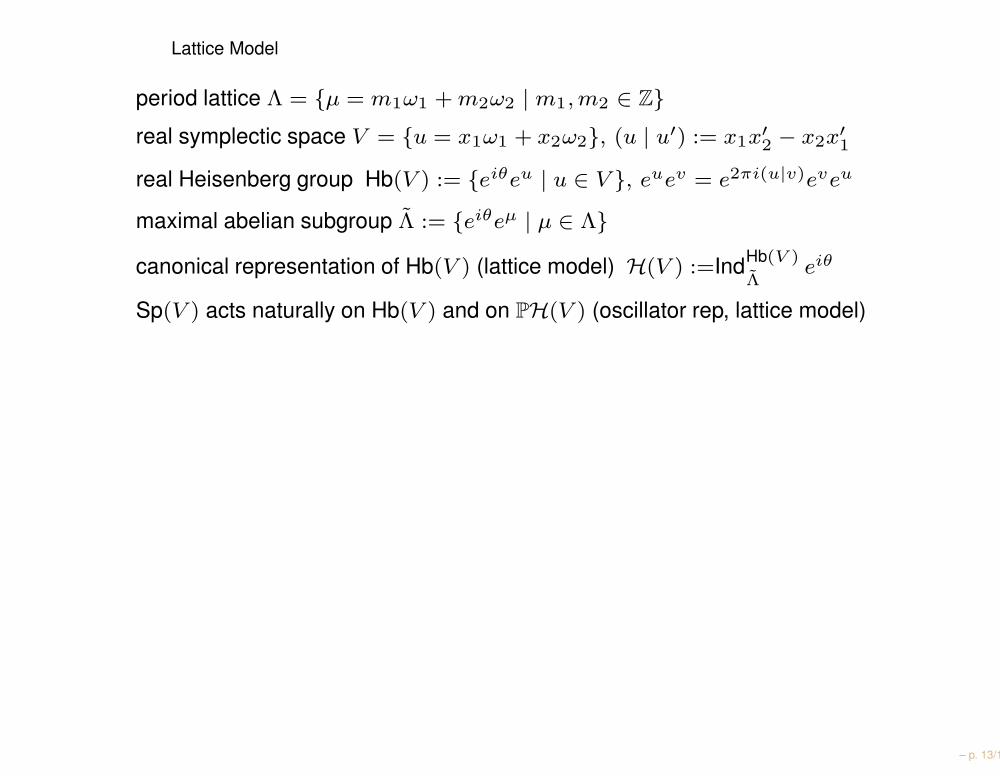
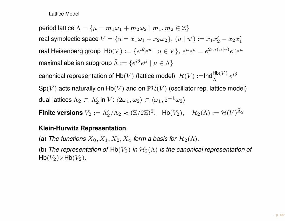
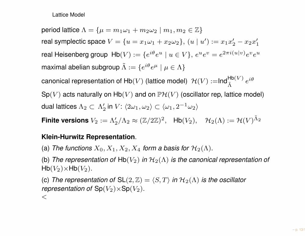
Lattice Model
period lattice Λ = µ = m1ω1 + m2ω2 | m1, m2 ∈ Z
real symplectic space V = u = x1ω1 + x2ω2, (u | u′) := x1x′2 − x2x′
1
real Heisenberg group Hb(V ) := eiθeu | u ∈ V , euev = e2πi(u|v)eveu
maximal abelian subgroup Λ := eiθeµ | µ ∈ Λ
canonical representation of Hb(V ) (lattice model) H(V ) :=IndHb(V )
Λeiθ
Sp(V ) acts naturally on Hb(V ) and on PH(V ) (oscillator rep, lattice model)
dual lattices Λ2 ⊂ Λ′2 in V : 〈2ω1, ω2〉 ⊂ 〈ω1, 2−1ω2〉
Finite versions V2 := Λ′2/Λ2 ≈ (Z/2Z)2, Hb(V2), H2(Λ) := H(V )Λ2
Klein-Hurwitz Representation.
(a) The functions X0, X1, X2, X4 form a basis for H2(Λ).
(b) The representation of Hb(V2) in H2(Λ) is the canonical representation ofHb(V2)×Hb(V2).
(c) The representation of SL(2, Z) = 〈S, T 〉 in H2(Λ) is the oscillatorrepresentation of Sp(V2)×Sp(V2).<
– p. 13/18
Lattice Model
period lattice Λ = µ = m1ω1 + m2ω2 | m1, m2 ∈ Zreal symplectic space V = u = x1ω1 + x2ω2, (u | u′) := x1x′
2 − x2x′1
real Heisenberg group Hb(V ) := eiθeu | u ∈ V , euev = e2πi(u|v)eveu
maximal abelian subgroup Λ := eiθeµ | µ ∈ Λ
canonical representation of Hb(V ) (lattice model) H(V ) :=IndHb(V )
Λeiθ
Sp(V ) acts naturally on Hb(V ) and on PH(V ) (oscillator rep, lattice model)
dual lattices Λ2 ⊂ Λ′2 in V : 〈2ω1, ω2〉 ⊂ 〈ω1, 2−1ω2〉
Finite versions V2 := Λ′2/Λ2 ≈ (Z/2Z)2, Hb(V2), H2(Λ) := H(V )Λ2
Klein-Hurwitz Representation.
(a) The functions X0, X1, X2, X4 form a basis for H2(Λ).
(b) The representation of Hb(V2) in H2(Λ) is the canonical representation ofHb(V2)×Hb(V2).
(c) The representation of SL(2, Z) = 〈S, T 〉 in H2(Λ) is the oscillatorrepresentation of Sp(V2)×Sp(V2).<
– p. 13/18
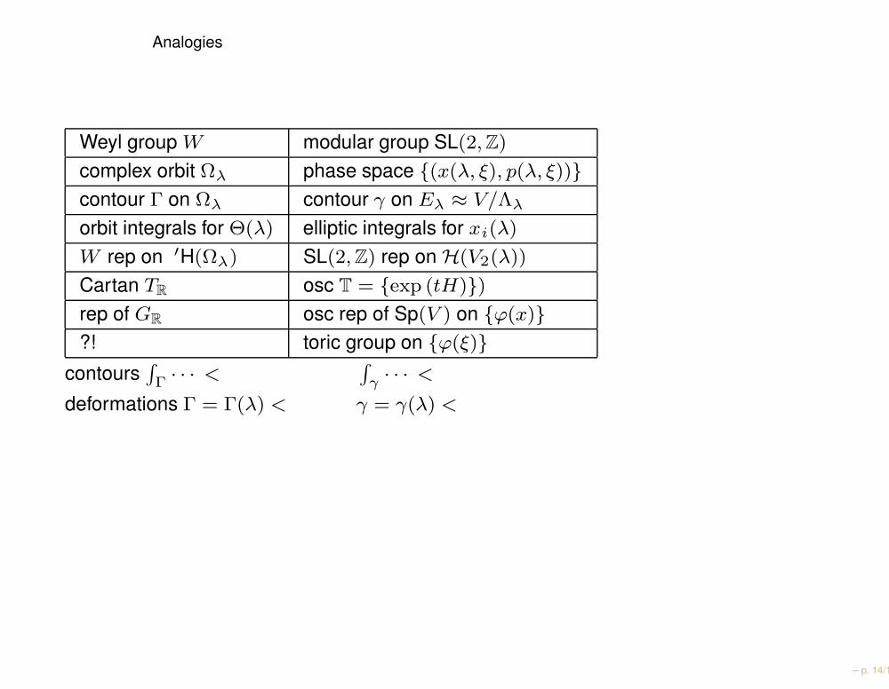
Analogies
Weyl group W modular group SL(2, Z)
complex orbit Ωλ phase space (x(λ, ξ), p(λ, ξ))contour Γ on Ωλ contour γ on Eλ ≈ V/Λλ
orbit integrals for Θ(λ) elliptic integrals for xi(λ)
W rep on ′H(Ωλ) SL(2, Z) rep on H(V2(λ))
Cartan TR osc T = exp (tH))rep of GR osc rep of Sp(V ) on ϕ(x)?! toric group on ϕ(ξ)
contours∫
Γ · · · <∫
γ · · · <
deformations Γ = Γ(λ) < γ = γ(λ) <
– p. 14/18
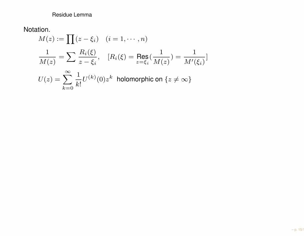
Residue Lemma
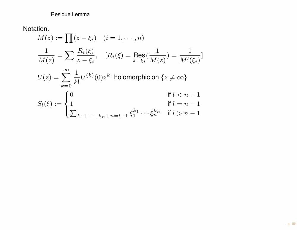
Notation.M(z) :=
∏
(z − ξi) (i = 1, · · · , n)
1
M(z)=
∑ Ri(ξ)
z − ξi, [Ri(ξ) = Res
z=ξi
(1
M(z)) =
1
M ′(ξi)]
U(z) =∞∑
k=0
1
k!U (k)(0)zk holomorphic on z 6= ∞
– p. 15/18
Residue Lemma
Notation.M(z) :=
∏
(z − ξi) (i = 1, · · · , n)
1
M(z)=
∑ Ri(ξ)
z − ξi, [Ri(ξ) = Res
z=ξi
(1
M(z)) =
1
M ′(ξi)]
U(z) =∞∑
k=0
1
k!U (k)(0)zk holomorphic on z 6= ∞
Sl(ξ) :=
0 if l < n − 1
1 if l = n − 1∑
k1+···+kn+n=l+1 ξk1
1 · · · ξknn if l > n − 1
– p. 15/18
Residue Lemma
Notation.M(z) :=
∏
(z − ξi) (i = 1, · · · , n)
1
M(z)=
∑ Ri(ξ)
z − ξi, [Ri(ξ) = Res
z=ξi
(1
M(z)) =
1
M ′(ξi)]
U(z) =∞∑
k=0
1
k!U (k)(0)zk holomorphic on z 6= ∞
Sl(ξ) :=
0 if l < n − 1
1 if l = n − 1∑
k1+···+kn+n=l+1 ξk1
1 · · · ξknn if l > n − 1
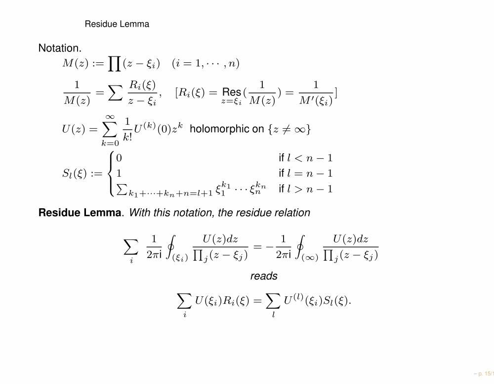
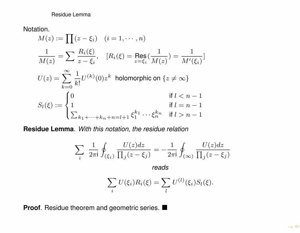
Residue Lemma. With this notation, the residue relation
∑
i
1
2πi
∮
(ξi)
U(z)dz∏
j(z − ξj)= − 1
2πi
∮
(∞)
U(z)dz∏
j(z − ξj)
reads∑
i
U(ξi)Ri(ξ) =∑
l
U (l)(ξi)Sl(ξ).
– p. 15/18
Residue Lemma
Notation.M(z) :=
∏
(z − ξi) (i = 1, · · · , n)
1
M(z)=
∑ Ri(ξ)
z − ξi, [Ri(ξ) = Res
z=ξi
(1
M(z)) =
1
M ′(ξi)]
U(z) =∞∑
k=0
1
k!U (k)(0)zk holomorphic on z 6= ∞
Sl(ξ) :=
0 if l < n − 1
1 if l = n − 1∑
k1+···+kn+n=l+1 ξk1
1 · · · ξknn if l > n − 1
Residue Lemma. With this notation, the residue relation
∑
i
1
2πi
∮
(ξi)
U(z)dz∏
j(z − ξj)= − 1
2πi
∮
(∞)
U(z)dz∏
j(z − ξj)
reads∑
i
U(ξi)Ri(ξ) =∑
l
U (l)(ξi)Sl(ξ).
Proof. Residue theorem and geometric series.
– p. 15/18
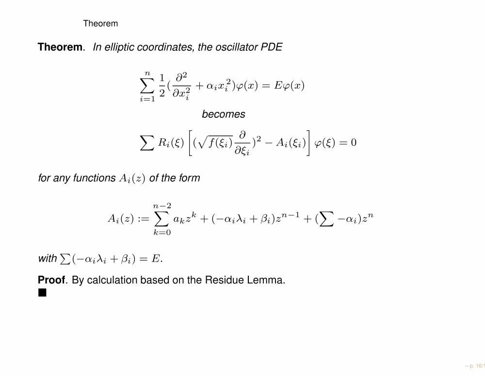
Theorem
Theorem. In elliptic coordinates, the oscillator PDE
n∑
i=1
1
2(
∂2
∂x2i
+ αix2i )ϕ(x) = Eϕ(x)
becomes
∑
Ri(ξ)
[
(√
f(ξi)∂
∂ξi)2 − Ai(ξi)
]
ϕ(ξ) = 0
for any functions Ai(z) of the form
Ai(z) :=
n−2∑
k=0
akzk + (−αiλi + βi)zn−1 + (
∑
−αi)zn
with∑
(−αiλi + βi) = E.
Proof. By calculation based on the Residue Lemma.
– p. 16/18
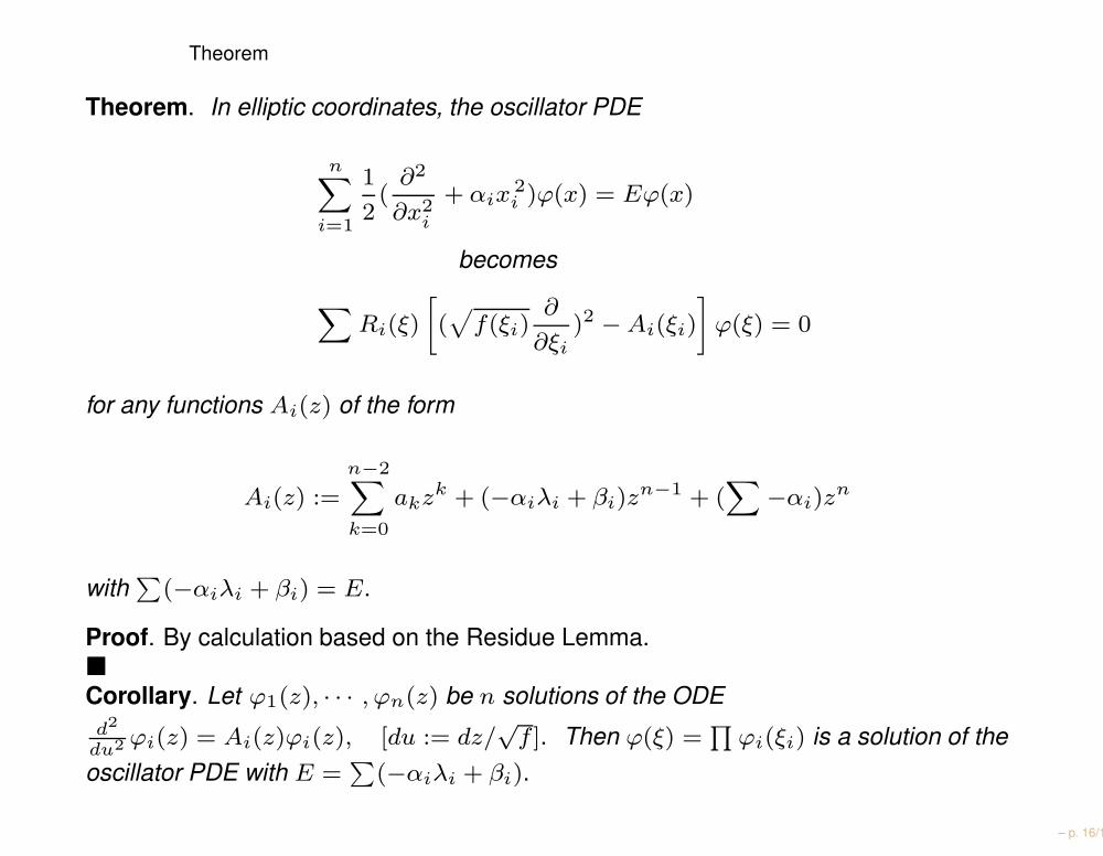
Theorem
Theorem. In elliptic coordinates, the oscillator PDE
n∑
i=1
1
2(
∂2
∂x2i
+ αix2i )ϕ(x) = Eϕ(x)
becomes
∑
Ri(ξ)
[
(√
f(ξi)∂
∂ξi)2 − Ai(ξi)
]
ϕ(ξ) = 0
for any functions Ai(z) of the form
Ai(z) :=
n−2∑
k=0
akzk + (−αiλi + βi)zn−1 + (
∑
−αi)zn
with∑
(−αiλi + βi) = E.
Proof. By calculation based on the Residue Lemma.
Corollary. Let ϕ1(z), · · · , ϕn(z) be n solutions of the ODEd2
du2ϕi(z) = Ai(z)ϕi(z), [du := dz/
√f ]. Then ϕ(ξ) =
∏
ϕi(ξi) is a solution of theoscillator PDE with E =
∑
(−αiλi + βi).
– p. 16/18
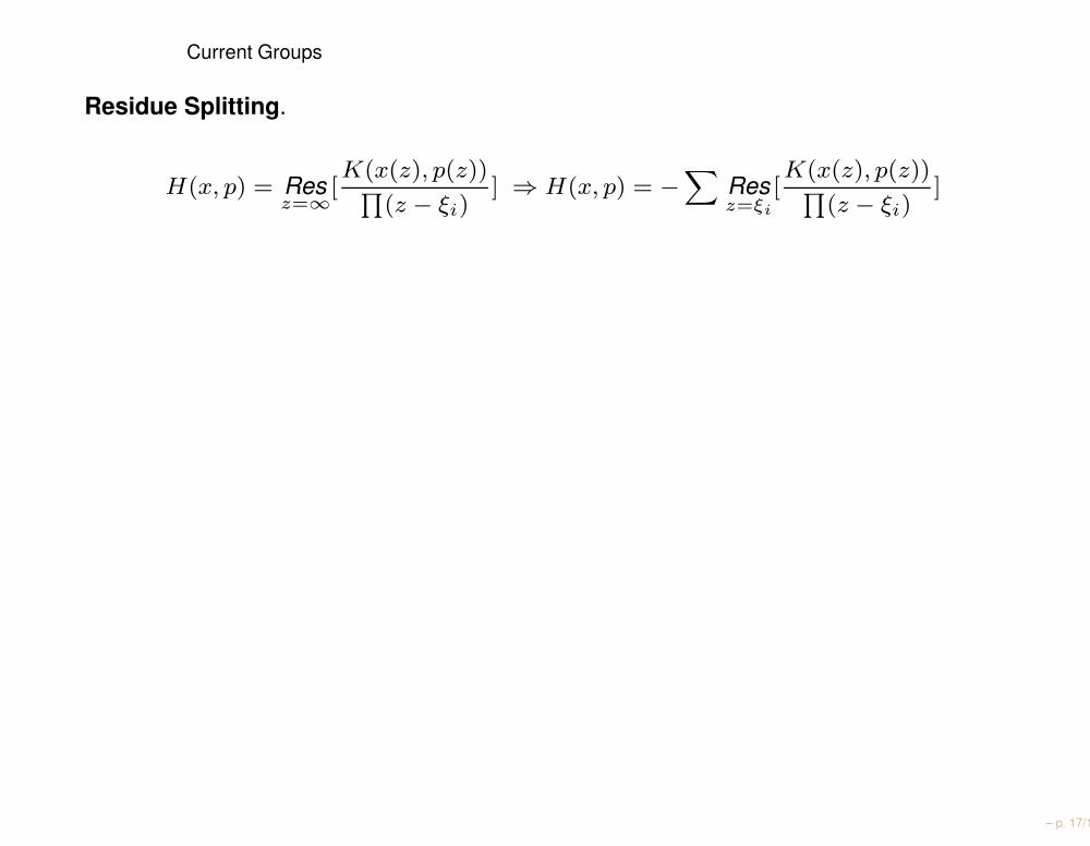
Current Groups
Residue Splitting.
H(x, p) = Resz=∞
[K(x(z), p(z))
∏
(z − ξi)] ⇒ H(x, p) = −
∑
Resz=ξi
[K(x(z), p(z))
∏
(z − ξi)]
– p. 17/18
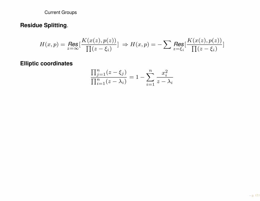
Current Groups
Residue Splitting.
H(x, p) = Resz=∞
[K(x(z), p(z))
∏
(z − ξi)] ⇒ H(x, p) = −
∑
Resz=ξi
[K(x(z), p(z))
∏
(z − ξi)]
Elliptic coordinates∏n
j=1(z − ξj)∏n
i=1(z − λi)= 1 −
n∑
i=1
x2i
z − λi
– p. 17/18
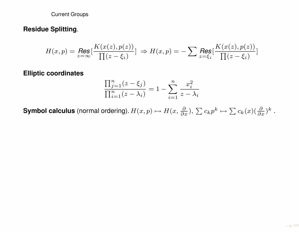
Current Groups
Residue Splitting.
H(x, p) = Resz=∞
[K(x(z), p(z))
∏
(z − ξi)] ⇒ H(x, p) = −
∑
Resz=ξi
[K(x(z), p(z))
∏
(z − ξi)]
Elliptic coordinates∏n
j=1(z − ξj)∏n
i=1(z − λi)= 1 −
n∑
i=1
x2i
z − λi
Symbol calculus (normal ordering). H(x, p) 7→ H(x, ∂∂x
),∑
ckpk 7→∑
ck(x)( ∂∂x
)k .
– p. 17/18
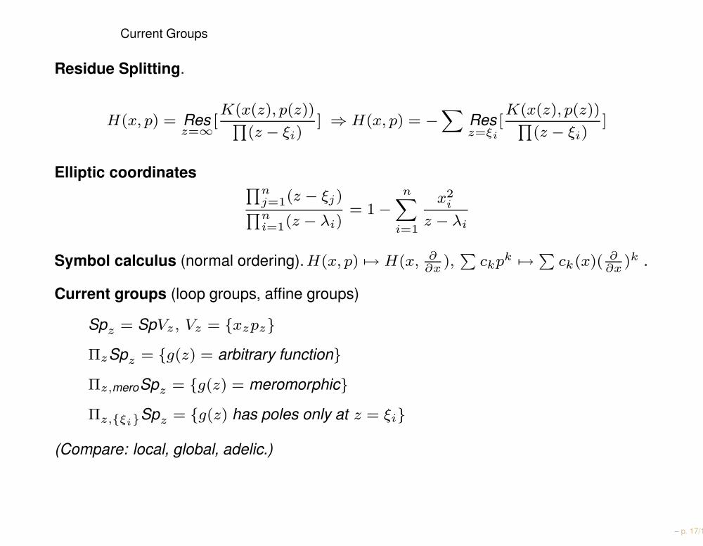
Current Groups
Residue Splitting.
H(x, p) = Resz=∞
[K(x(z), p(z))
∏
(z − ξi)] ⇒ H(x, p) = −
∑
Resz=ξi
[K(x(z), p(z))
∏
(z − ξi)]
Elliptic coordinates∏n
j=1(z − ξj)∏n
i=1(z − λi)= 1 −
n∑
i=1
x2i
z − λi
Symbol calculus (normal ordering). H(x, p) 7→ H(x, ∂∂x
),∑
ckpk 7→∑
ck(x)( ∂∂x
)k .
Current groups (loop groups, affine groups)
Spz = SpVz, Vz = xzpz
ΠzSpz = g(z) = arbitrary function
Πz,meroSpz = g(z) = meromorphic
Πz,ξiSpz = g(z) has poles only at z = ξi
(Compare: local, global, adelic.)
– p. 17/18
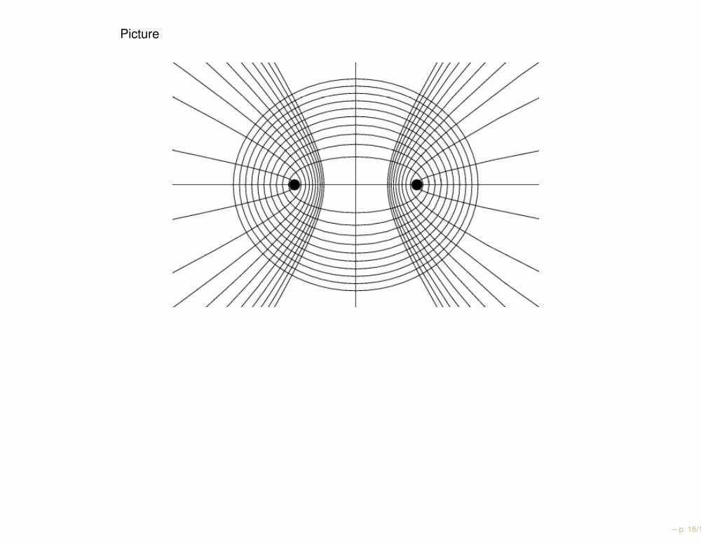
Picture
– p. 18/18
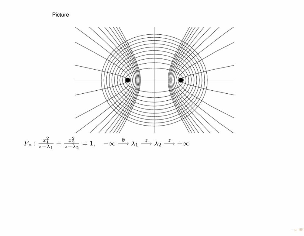
Picture
Fz :x2
1
z−λ1+
x2
2
z−λ2= 1, −∞ ∅−→ λ1
z−→ λ2z−→ +∞
– p. 18/18

Picture
Fz :x2
1
z−λ1+
x2
2
z−λ2= 1, −∞ ∅−→ λ1
z−→ λ2z−→ +∞
– p. 18/18
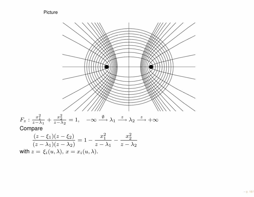
Picture
Fz :x2
1
z−λ1+
x2
2
z−λ2= 1, −∞ ∅−→ λ1
z−→ λ2z−→ +∞
Compare(z − ξ1)(z − ξ2)
(z − λ1)(z − λ2)= 1 − x2
1
z − λ1− x2
2
z − λ2
with z = ξi(u, λ), x = xi(u, λ).
– p. 18/18