Ridge&Regression - University of Chicagottic.uchicago.edu/~ryotat/teaching/enshu12.pdfwhere w¯...
52
Ridge Regression Ryota Tomioka Department of Mathema6cal Informa6cs The University of Tokyo
Transcript of Ridge&Regression - University of Chicagottic.uchicago.edu/~ryotat/teaching/enshu12.pdfwhere w¯...
Ridge Regression
Ryota Tomioka Department of Mathema6cal Informa6cs
The University of Tokyo

About this class
• Bad news: This class will be in English. • Good news: The topic “ridge regression” is probably already familiar to you.
• Even beGer news: if you ask a ques6on in English during the class, then you don’t need to hand in any assignment (no report) for this class.
# Of course you can s6ll ask ques6ons in Japanese but you have to hand in your assignment as usual.
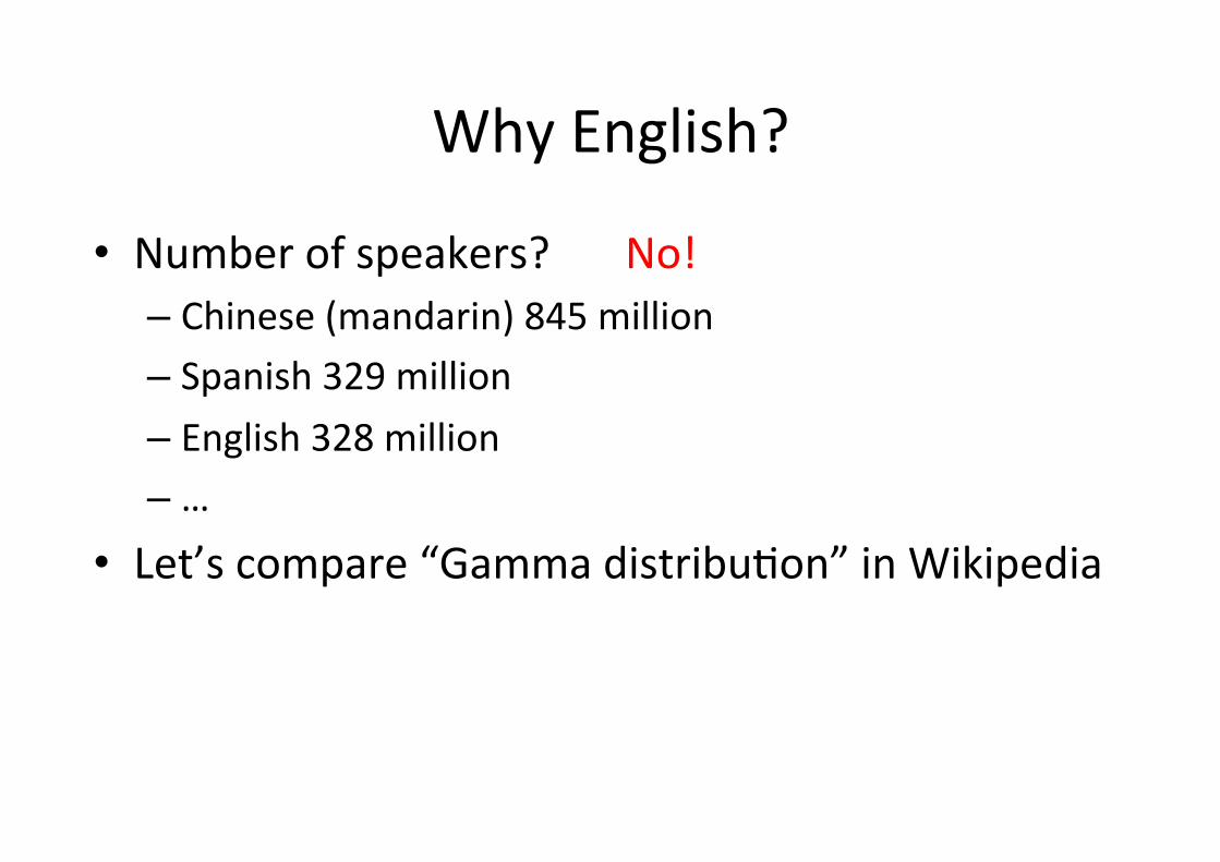
Why English?
• Number of speakers? – Chinese (mandarin) 845 million – Spanish 329 million – English 328 million – …
• Let’s compare “Gamma distribu6on” in Wikipedia
No!
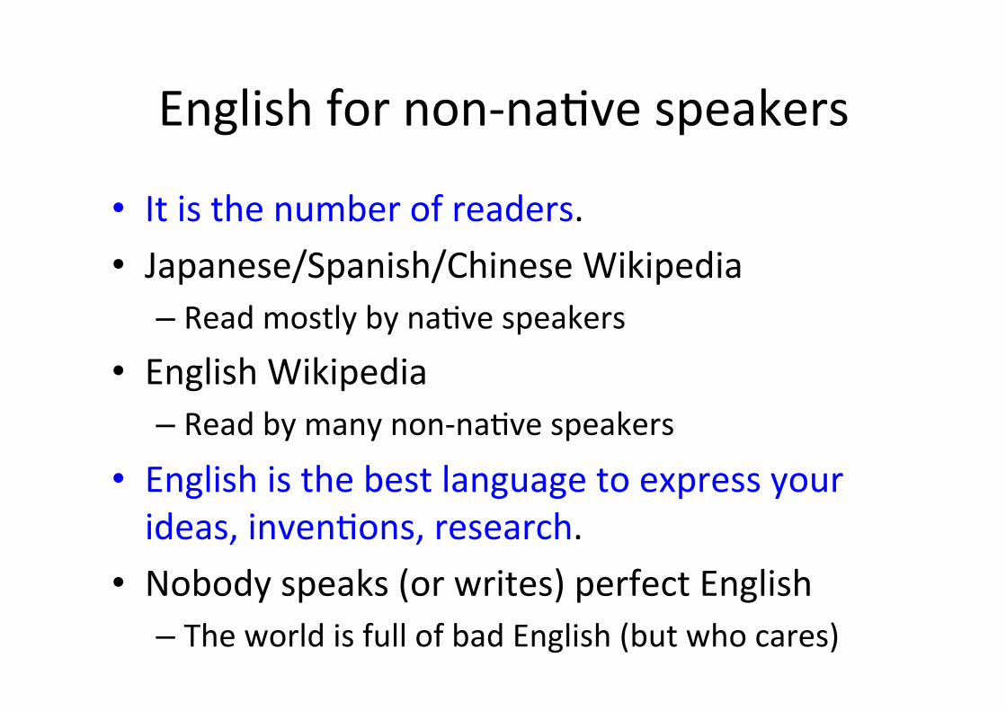
English for non-‐na6ve speakers
• It is the number of readers. • Japanese/Spanish/Chinese Wikipedia – Read mostly by na6ve speakers
• English Wikipedia – Read by many non-‐na6ve speakers
• English is the best language to express your ideas, inven6ons, research.
• Nobody speaks (or writes) perfect English – The world is full of bad English (but who cares)

Outline
• Ridge Regression (regularized linear regression) – Formula6on – Handling Nonlinearity using basis func6ons – Classifica6on – Mul6-‐class classifica6on
• Singularity ― the dark side of RR – Why does it happen? – How can we avoid it?
• Summary
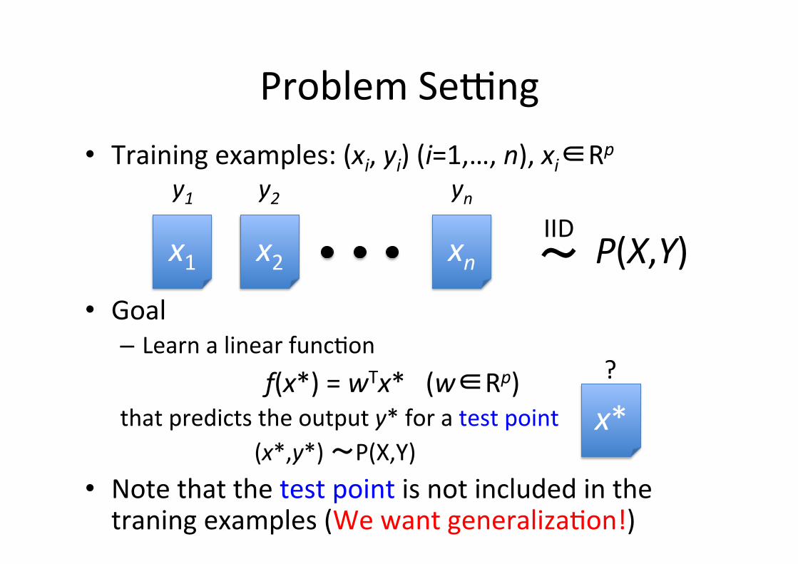
Problem Segng • Training examples: (xi, yi) (i=1,…, n), xi∈Rp
• Goal – Learn a linear func6on f(x*) = wTx* (w∈Rp) that predicts the output y* for a test point (x*,y*) ~P(X,Y)
• Note that the test point is not included in the traning examples (We want generaliza6on!)
x1 x2 xn
y1 y2 yn
P(X,Y) ~ IID
x*
?
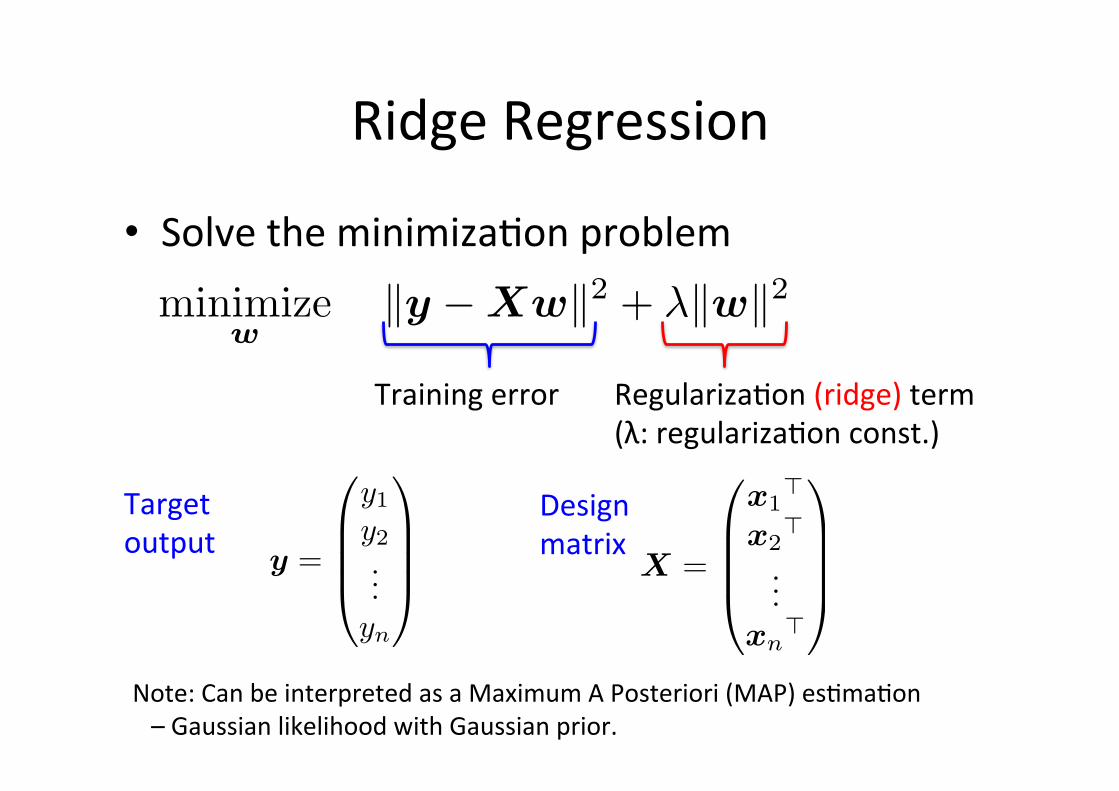
Ridge Regression
• Solve the minimiza6on problem
minimizew
�y −Xw�2 + λ�w�2
Training error Regulariza6on (ridge) term (λ: regulariza6on const.)
Note: Can be interpreted as a Maximum A Posteriori (MAP) es6ma6on – Gaussian likelihood with Gaussian prior.
y =
y1
y2...
yn
X =
x1�
x2�
...xn�
Target output
Design matrix
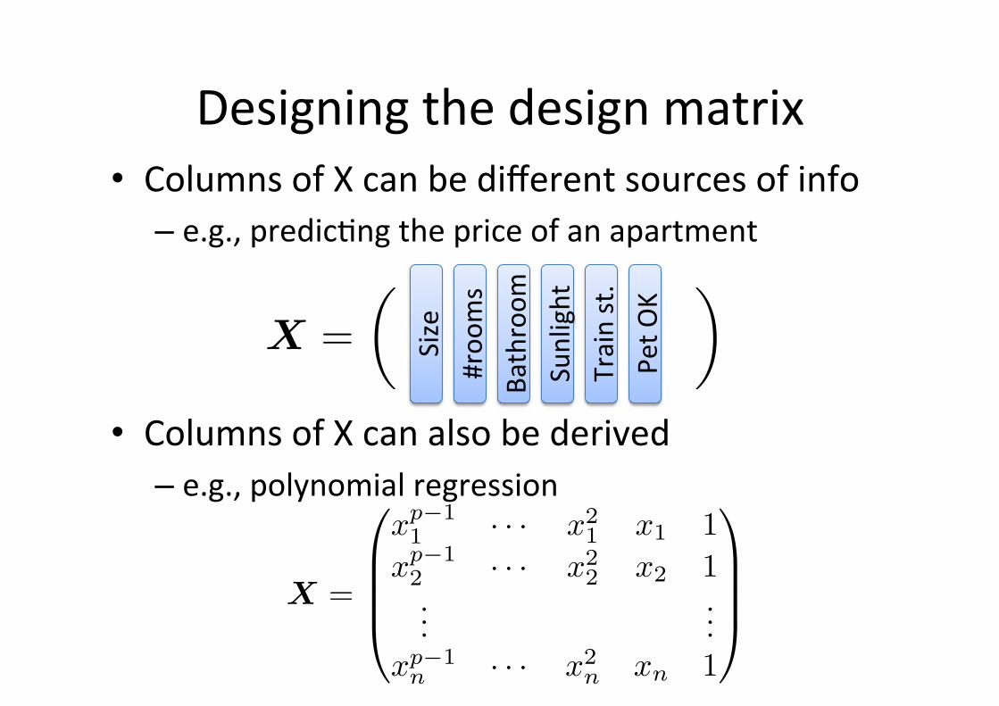
Designing the design matrix • Columns of X can be different sources of info – e.g., predic6ng the price of an apartment
• Columns of X can also be derived – e.g., polynomial regression
#roo
ms
Train st.
Size
Bathroom
Sunlight
Pet O
K
X =� �
X =
xp−11 · · · x2
1 x1 1xp−1
2 · · · x22 x2 1
......
xp−1n · · · x2
n xn 1
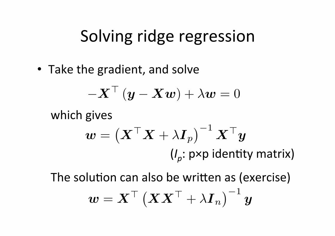
Solving ridge regression
• Take the gradient, and solve
−X� (y −Xw) + λw = 0
which gives
(Ip: p×p iden6ty matrix)
The solu6on can also be wriGen as (exercise)
w =�X�X + λIp
�−1X�y
w = X� �XX� + λIn
�−1y
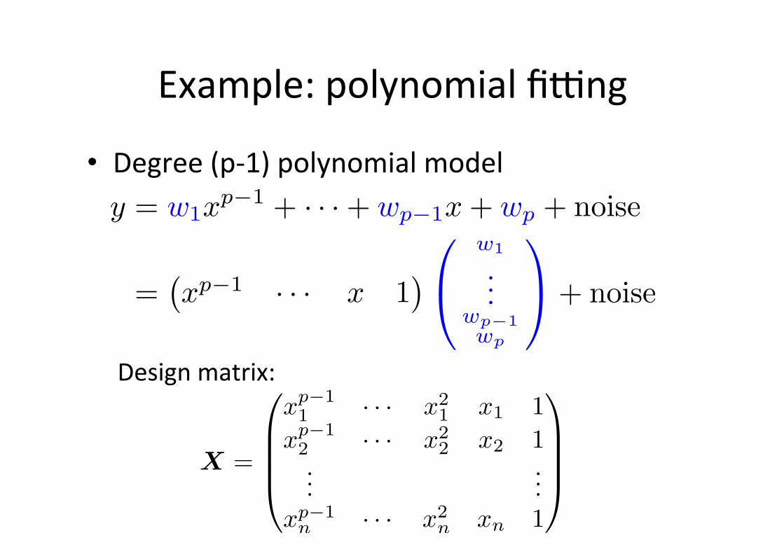
Example: polynomial figng
• Degree (p-‐1) polynomial model
Design matrix:
y = w1xp−1 + · · · + wp−1x + wp + noise
=�xp−1 · · · x 1
�
w1
...wp−1wp
+ noise
X =
xp−11 · · · x2
1 x1 1xp−1
2 · · · x22 x2 1
......
xp−1n · · · x2
n xn 1
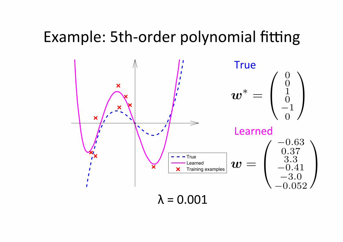
Example: 5th-‐order polynomial figng
True
Learned
Training examples
True
w∗ =
0010−10
Learned
w =
−0.630.373.3−0.41−3.0−0.052
λ = 0.001
µ1
µ2
µ3
µ4
µ5
µ6
µ7
µ8
µ9
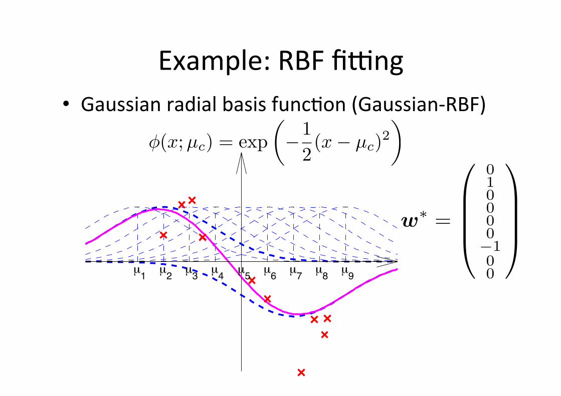
Example: RBF figng • Gaussian radial basis func6on (Gaussian-‐RBF)
φ(x;µc) = exp�−1
2(x− µc)2
�
w∗ =
010000−100
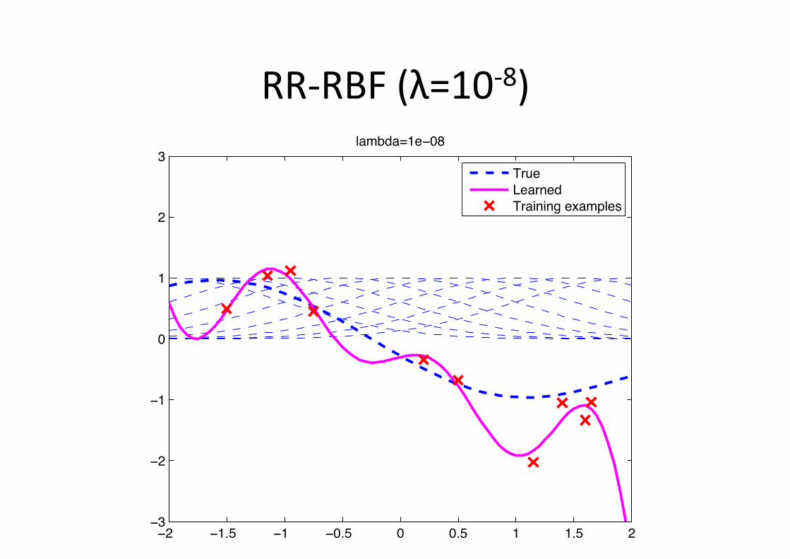
RR-‐RBF (λ=10-‐8)
!! !"#$ !" !%#$ % %#$ " "#$ !!&
!!
!"
%
"
!
&'()*+(,"-!%.
/
/
012-
3-(14-+
01(54546/-7()8'-9
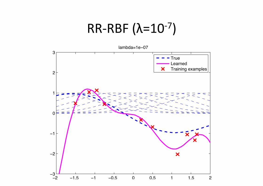
RR-‐RBF (λ=10-‐7)
!! !"#$ !" !%#$ % %#$ " "#$ !!&
!!
!"
%
"
!
&'()*+(,"-!%.
/
/
012-
3-(14-+
01(54546/-7()8'-9

RR-‐RBF (λ=10-‐6)
!! !"#$ !" !%#$ % %#$ " "#$ !!&
!!
!"
%
"
!
&'()*+(,"-!%.
/
/
012-
3-(14-+
01(54546/-7()8'-9
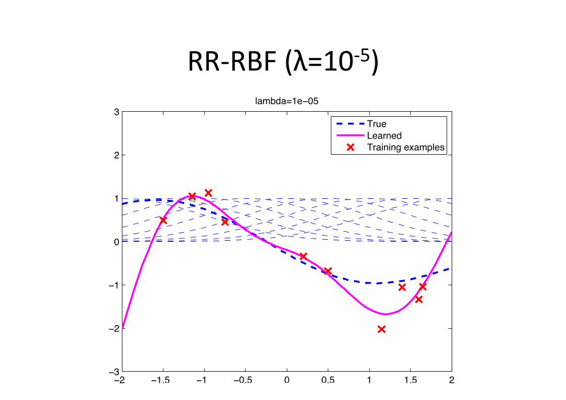
RR-‐RBF (λ=10-‐5)
!! !"#$ !" !%#$ % %#$ " "#$ !!&
!!
!"
%
"
!
&'()*+(,"-!%$
.
.
/01-
2-(03-+
/0(43435.-6()7'-8

RR-‐RBF (λ=10-‐4)
!! !"#$ !" !%#$ % %#$ " "#$ !!&
!!
!"
%
"
!
&'()*+(,%#%%%"
-
-
./01
21(/31+
./(43435-16()7'18
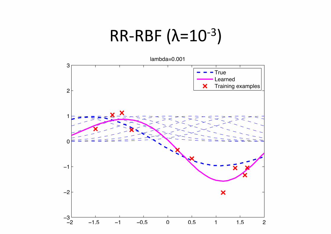
RR-‐RBF (λ=10-‐3)
!! !"#$ !" !%#$ % %#$ " "#$ !!&
!!
!"
%
"
!
&'()*+(,%#%%"
-
-
./01
21(/31+
./(43435-16()7'18

RR-‐RBF (λ=10-‐2)
!! !"#$ !" !%#$ % %#$ " "#$ !!&
!!
!"
%
"
!
&'()*+(,%#%"
-
-
./01
21(/31+
./(43435-16()7'18

RR-‐RBF (λ=10-‐1)
!! !"#$ !" !%#$ % %#$ " "#$ !!&
!!
!"
%
"
!
&'()*+(,%#"
-
-
./01
21(/31+
./(43435-16()7'18
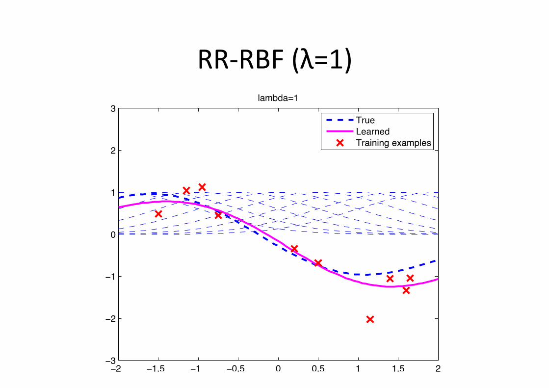
RR-‐RBF (λ=1)
!! !"#$ !" !%#$ % %#$ " "#$ !!&
!!
!"
%
"
!
&'()*+(,"
-
-
./01
21(/31+
./(43435-16()7'18
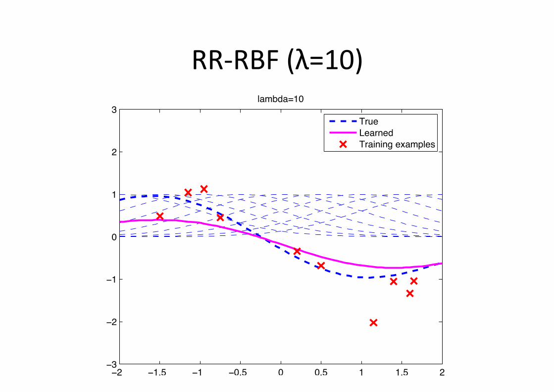
RR-‐RBF (λ=10)
!! !"#$ !" !%#$ % %#$ " "#$ !!&
!!
!"
%
"
!
&'()*+(,"%
-
-
./01
21(/31+
./(43435-16()7'18
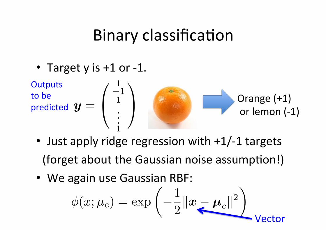
Binary classifica6on
• Target y is +1 or -‐1.
• Just apply ridge regression with +1/-‐1 targets (forget about the Gaussian noise assump6on!) • We again use Gaussian RBF:
Orange (+1) or lemon (-‐1)
φ(x;µc) = exp�−1
2�x− µc�2
�
Vector
y =
1−11...1
Outputs to be predicted
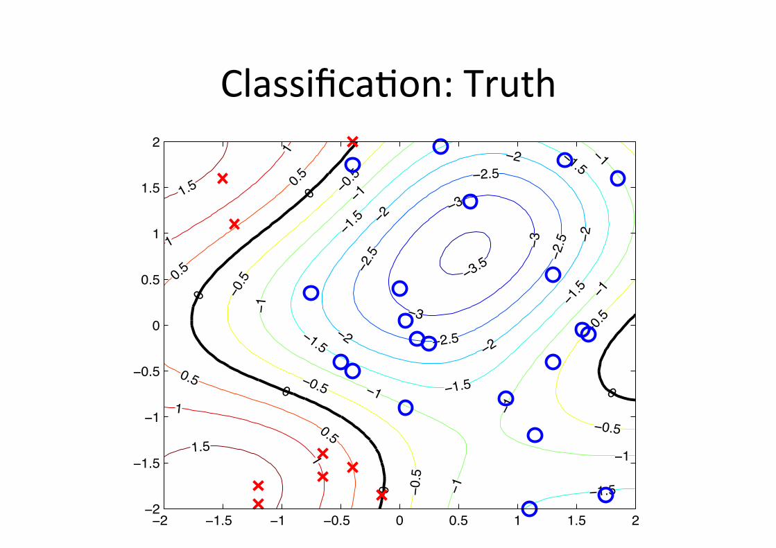
Classifica6on: Truth
!!"#
!!
!!
!!
!$"#
!$"#
!$"#
!$"#
!$
!$
!$
!$
!$!
%"#
!%"#
!%"#
!%"#
!%"#
!%"#
!%
!%
!%
!%
!%
!%
!%
!%
!&"#
!&"#
!&"#
!&"#
!&"#
!&"#
&&
&&
&
&"#
&"#
&"#
&"#
%
%
%
%
%"#
%"#
!$ !%"# !% !&"# & &"# % %"# $!$
!%"#
!%
!&"#
&
&"#
%
%"#
$
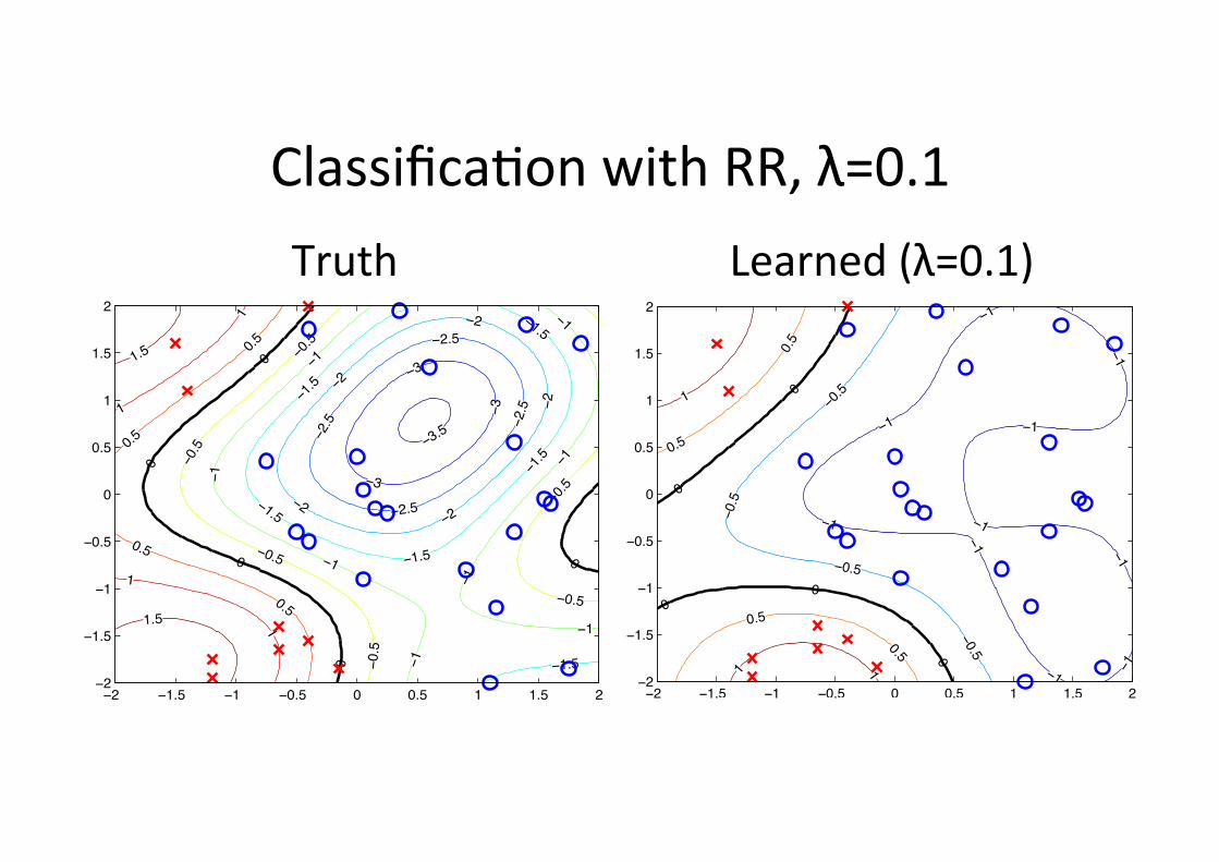
Classifica6on with RR, λ=0.1
!!
!!
!!
!!
!!
!!
!!
!!
!!
!!
!"#$
!"#$
!"#$
!"#$
"
"
"
"
"
"#$
"#$
"#$
"#$
! !
!
!% !!#$ !! !"#$ " "#$ ! !#$ %!%
!!#$
!!
!"#$
"
"#$
!
!#$
%
!!"#
!!
!!!!
!$"#
!$"#
!$"#!$"#
!$
!$
!$
!$
!$!
%"#
!%"#
!%"#
!%"#
!%"#
!%"#
!%
!%
!%
!%
!%
!%
!%
!%
!&"#
!&"#
!&"#
!&"#
!&"#
!&"#
&
&
&
&
&
&"#
&"#
&"#
&"#
%
%
%
%
%"#
%"#
!$ !%"# !% !&"# & &"# % %"# $!$
!%"#
!%
!&"#
&
&"#
%
%"#
$
Truth Learned (λ=0.1)
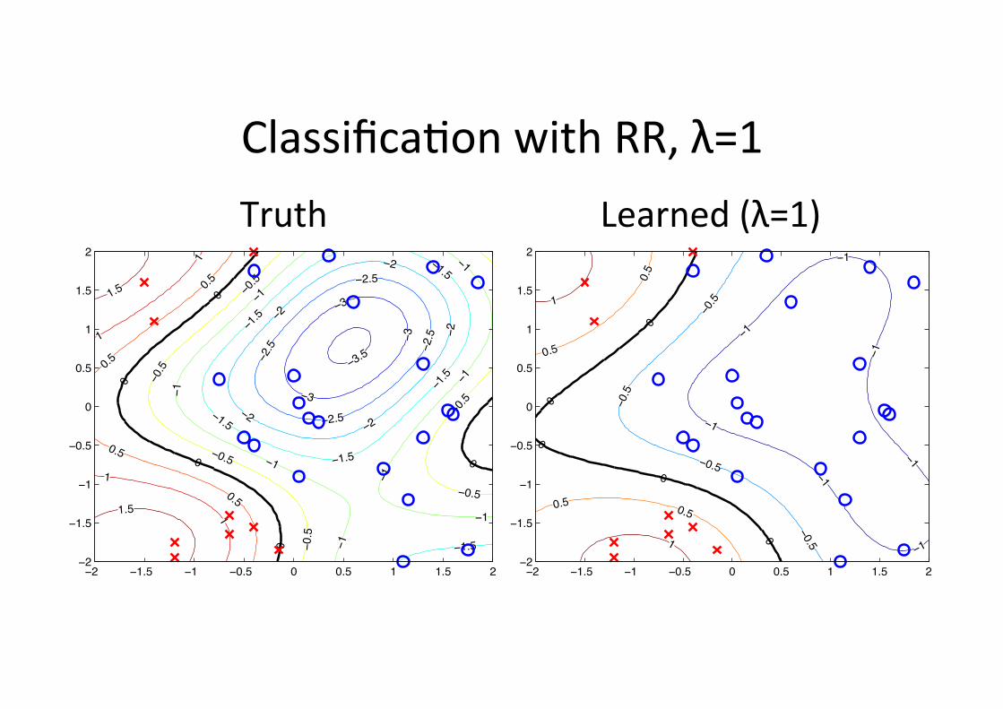
Classifica6on with RR, λ=1
!!"#
!!
!!!!
!$"#
!$"#
!$"#!$"#
!$
!$
!$
!$
!$!
%"#
!%"#
!%"#
!%"#
!%"#
!%"#
!%
!%
!%
!%
!%
!%
!%
!%
!&"#
!&"#
!&"#
!&"#
!&"#
!&"#
&
&
&
&
&
&"#
&"#
&"#
&"#
%
%
%
%
%"#
%"#
!$ !%"# !% !&"# & &"# % %"# $!$
!%"#
!%
!&"#
&
&"#
%
%"#
$
Truth Learned (λ=1)
!!
!!
!!
!!
!!
!!
!!
!"#$
!"#$
!"#$
!"#$
"
"
"
"
"
"#$
"#$
"#$"#$
!
!
!% !!#$ !! !"#$ " "#$ ! !#$ %!%
!!#$
!!
!"#$
"
"#$
!
!#$
%
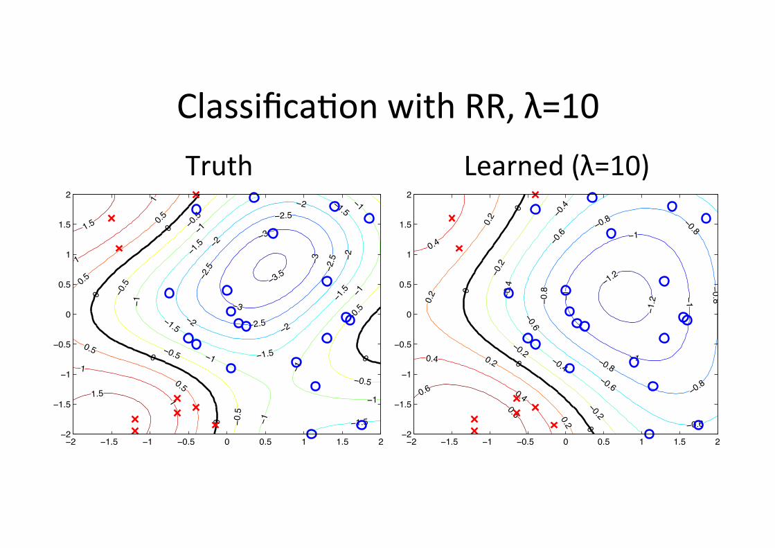
Classifica6on with RR, λ=10
!!"#
!!
!!!!
!$"#
!$"#
!$"#!$"#
!$
!$
!$
!$
!$!
%"#
!%"#
!%"#
!%"#
!%"#
!%"#
!%
!%
!%
!%
!%
!%
!%
!%
!&"#
!&"#
!&"#
!&"#
!&"#
!&"#
&
&
&
&
&
&"#
&"#
&"#
&"#
%
%
%
%
%"#
%"#
!$ !%"# !% !&"# & &"# % %"# $!$
!%"#
!%
!&"#
&
&"#
%
%"#
$
Truth Learned (λ=10)
!!"#
!!"#
!!
!!
!!
!!
!$"%
!$"%
!$"%
!$"%
!$"%
!$"%
!$"&
!$"&
!$"&
!$"&
!$"'
!$"'
!$"'
!$"#
!$"#
!$"#
$
$
$
$
$"#
$"#
$"#
$"#
$"'
$"'
$"'
$"&
$"&
!# !!"( !! !$"( $ $"( ! !"( #!#
!!"(
!!
!$"(
$
$"(
!
!"(
#
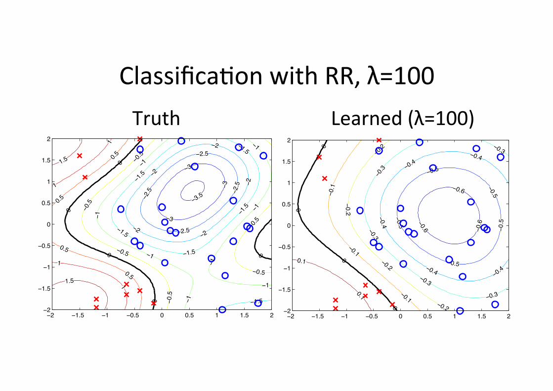
Classifica6on with RR, λ=100
!!"#
!!
!!!!
!$"#
!$"#
!$"#!$"#
!$
!$
!$
!$
!$!
%"#
!%"#
!%"#
!%"#
!%"#
!%"#
!%
!%
!%
!%
!%
!%
!%
!%
!&"#
!&"#
!&"#
!&"#
!&"#
!&"#
&
&
&
&
&
&"#
&"#
&"#
&"#
%
%
%
%
%"#
%"#
!$ !%"# !% !&"# & &"# % %"# $!$
!%"#
!%
!&"#
&
&"#
%
%"#
$
Truth Learned (λ=100)
!!"#
!!"# !
!"#
!!"$
!!"$
!!"$
!!"$
!!"$
!!"%
!!"%
!!"%
!!"%!!"%
!!"&
!!"&
!!"&
!!"&
!!"&!!"'
!!"'
!!"'
!!"'
!!"(
!!"(
!!"(
!
!!
!
!"(
!"(
!' !("$ !( !!"$ ! !"$ ( ("$ '!'
!("$
!(
!!"$
!
!"$
(
("$
'
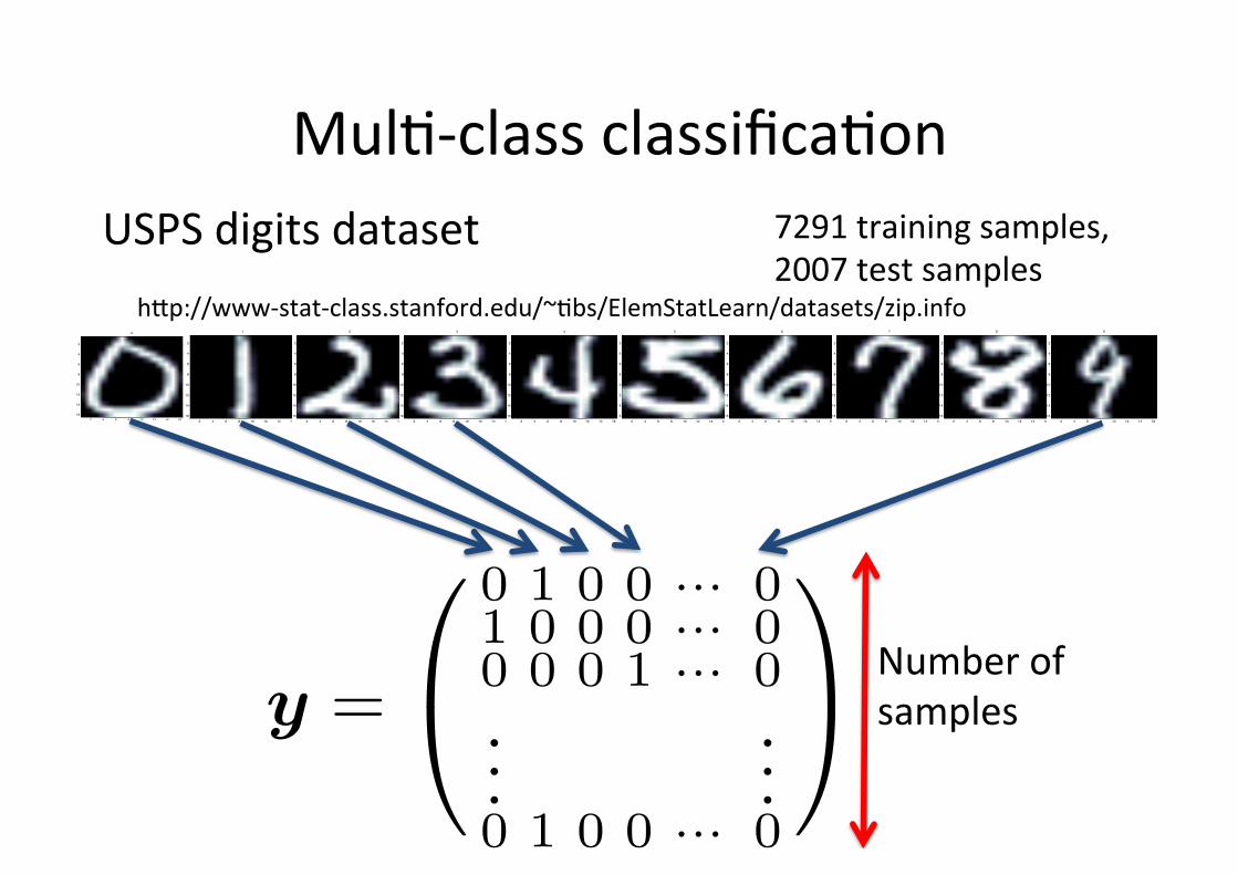
Mul6-‐class classifica6on
0
2 4 6 8 10 12 14 16
2
4
6
8
10
12
14
16
5
2 4 6 8 10 12 14 16
2
4
6
8
10
12
14
16
1
2 4 6 8 10 12 14 16
2
4
6
8
10
12
14
16
2
2 4 6 8 10 12 14 16
2
4
6
8
10
12
14
16
3
2 4 6 8 10 12 14 16
2
4
6
8
10
12
14
16
4
2 4 6 8 10 12 14 16
2
4
6
8
10
12
14
16
6
2 4 6 8 10 12 14 16
2
4
6
8
10
12
14
16
7
2 4 6 8 10 12 14 16
2
4
6
8
10
12
14
16
8
2 4 6 8 10 12 14 16
2
4
6
8
10
12
14
16
9
2 4 6 8 10 12 14 16
2
4
6
8
10
12
14
16
USPS digits dataset hGp://www-‐stat-‐class.stanford.edu/~6bs/ElemStatLearn/datasets/zip.info
y =
0 1 0 0 ··· 01 0 0 0 ··· 00 0 0 1 ··· 0...
...0 1 0 0 ··· 0
Number of samples
7291 training samples, 2007 test samples
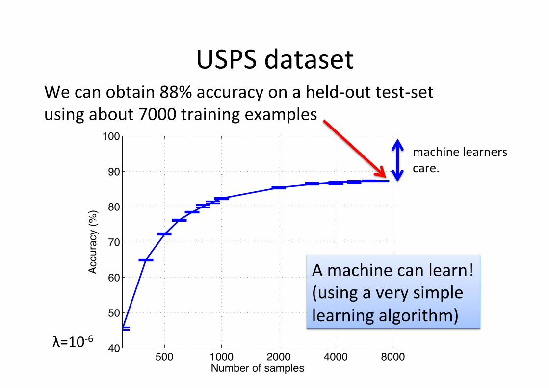
500 1000 2000 4000 800040
50
60
70
80
90
100
Number of samples
Accu
racy (
%)
USPS dataset We can obtain 88% accuracy on a held-‐out test-‐set using about 7000 training examples
A machine can learn! (using a very simple learning algorithm)
machine learners care.
λ=10-‐6
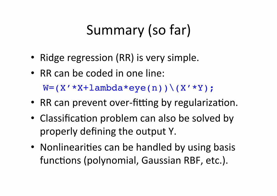
Summary (so far)
• Ridge regression (RR) is very simple. • RR can be coded in one line:
W=(X’*X+lambda*eye(n))\(X’*Y);!
• RR can prevent over-‐figng by regulariza6on. • Classifica6on problem can also be solved by properly defining the output Y.
• Nonlineari6es can be handled by using basis func6ons (polynomial, Gaussian RBF, etc.).
Singularity -‐ The dark side of RR
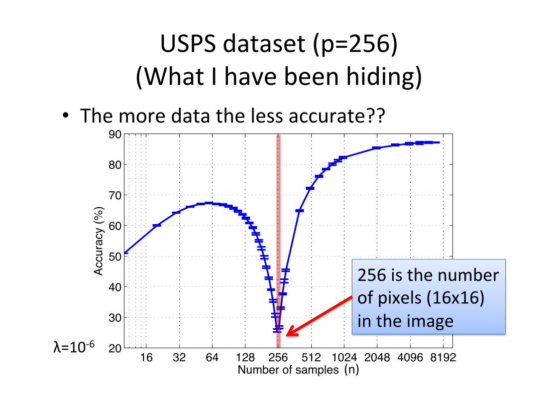
USPS dataset (p=256) (What I have been hiding)
• The more data the less accurate??
16 32 64 128 256 512 1024 2048 4096 819220
30
40
50
60
70
80
90
Number of samples
Accura
cy (
%)
256 is the number of pixels (16x16) in the image
(n) λ=10-‐6
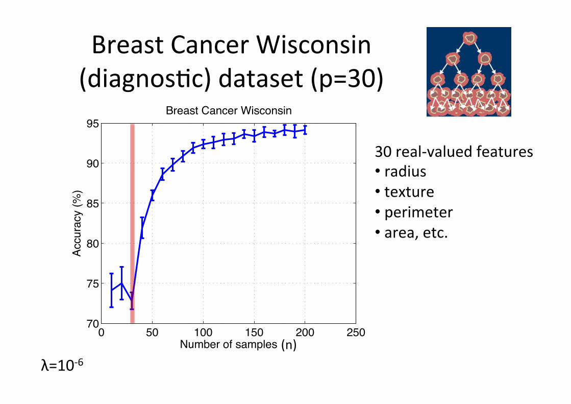
Breast Cancer Wisconsin (diagnos6c) dataset (p=30)
0 50 100 150 200 25070
75
80
85
90
95
Number of samples
Accura
cy (
%)
Breast Cancer Wisconsin
(n) λ=10-‐6
30 real-‐valued features • radius • texture • perimeter • area, etc.
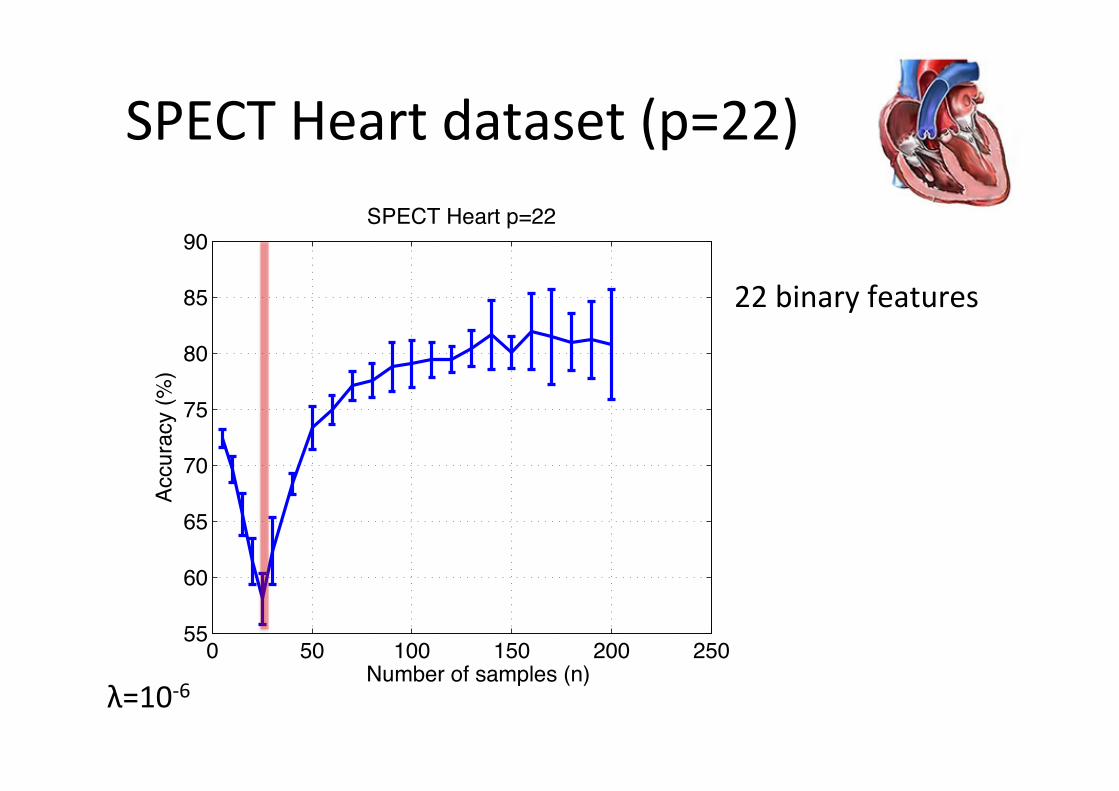
SPECT Heart dataset (p=22)
0 50 100 150 200 25055
60
65
70
75
80
85
90
Number of samples (n)
Accura
cy (
%)
SPECT Heart p=22
λ=10-‐6
22 binary features
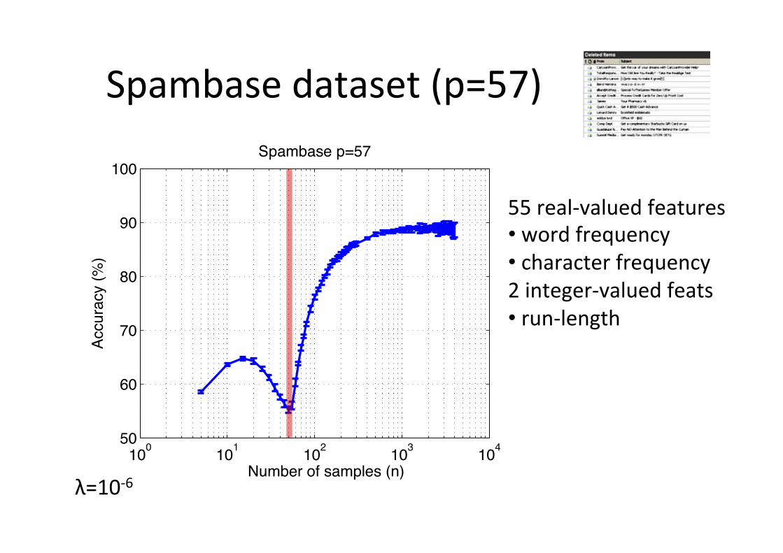
Spambase dataset (p=57)
100
101
102
103
104
50
60
70
80
90
100
Number of samples (n)
Accura
cy (
%)
Spambase p=57
λ=10-‐6
55 real-‐valued features • word frequency • character frequency 2 integer-‐valued feats • run-‐length
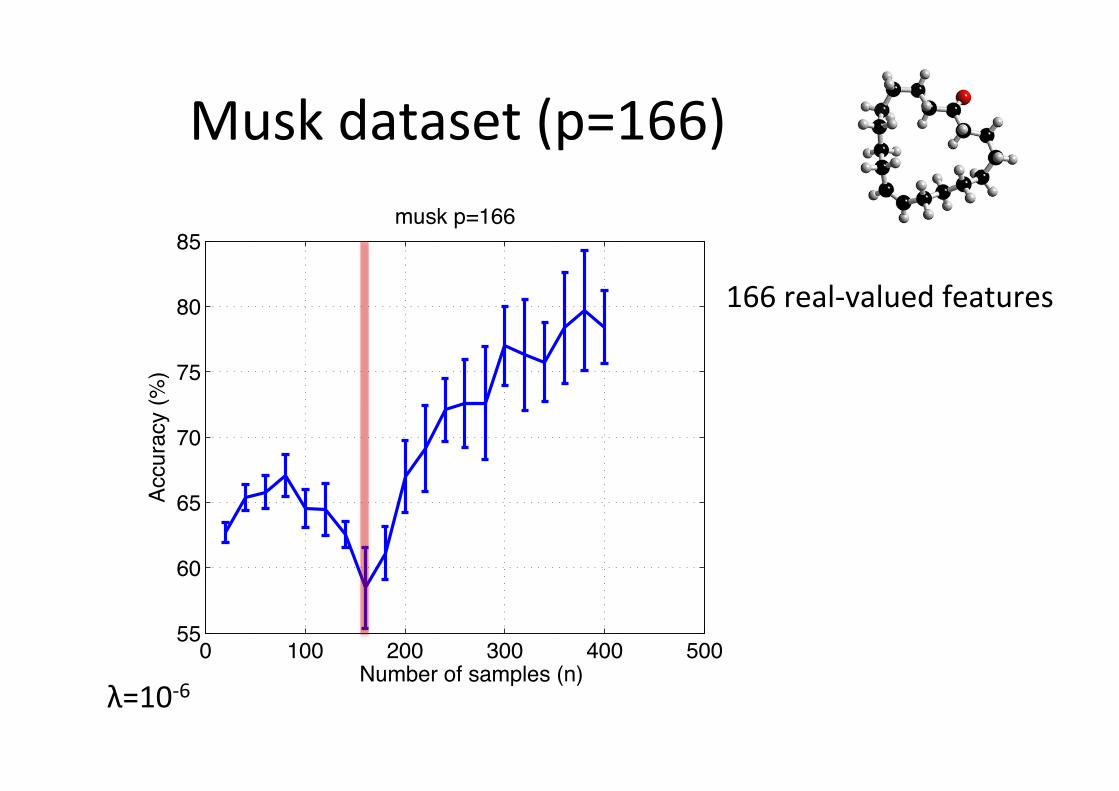
Musk dataset (p=166)
0 100 200 300 400 50055
60
65
70
75
80
85
Number of samples (n)
Accura
cy (
%)
musk p=166
λ=10-‐6
166 real-‐valued features
Singularity
Why does it happen? How can we avoid it?
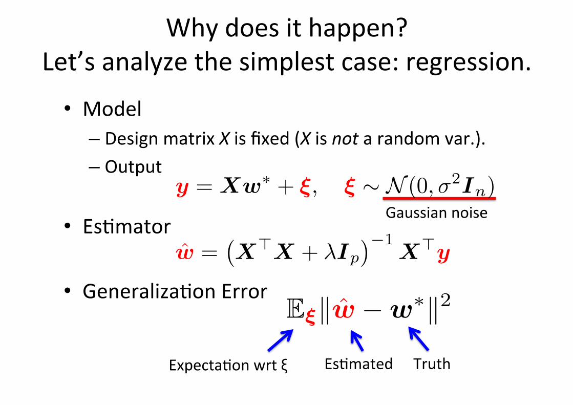
Why does it happen? Let’s analyze the simplest case: regression.
• Model – Design matrix X is fixed (X is not a random var.). – Output
• Es6mator • Generaliza6on Error
Gaussian noise
Es6mated Truth
y = Xw∗ + ξ, ξ ∼ N (0,σ2In)
Eξ�w −w∗�2
w =�X�X + λIp
�−1X�y
Expecta6on wrt ξ
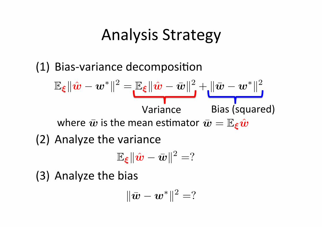
Analysis Strategy
(1) Bias-‐variance decomposi6on
(2) Analyze the variance
(3) Analyze the bias
Eξ�w −w∗�2 = Eξ�w − w�2 + �w −w∗�2
Variance Bias (squared) w = Eξwwwhere is the mean es6mator
Eξ�w − w�2 =?
�w −w∗�2 =?
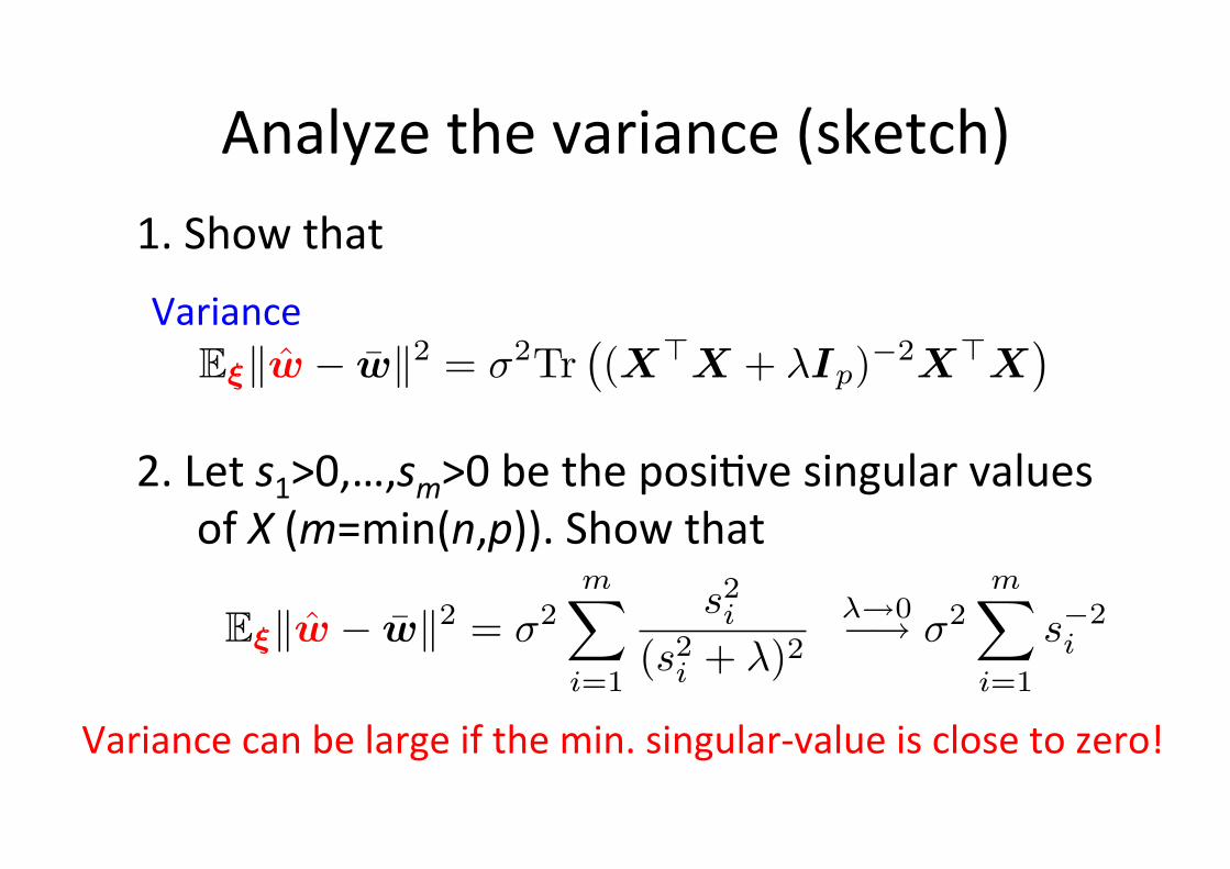
Analyze the variance (sketch)
2. Let s1>0,…,sm>0 be the posi6ve singular values of X (m=min(n,p)). Show that
Eξ�w − w�2 = σ2Tr�(X�X + λIp)−2X�X
�
1. Show that
Eξ�w − w�2 = σ2m�
i=1
s2i
(s2i + λ)2
λ→0−→ σ2m�
i=1
s−2i
Variance can be large if the min. singular-‐value is close to zero!
Variance
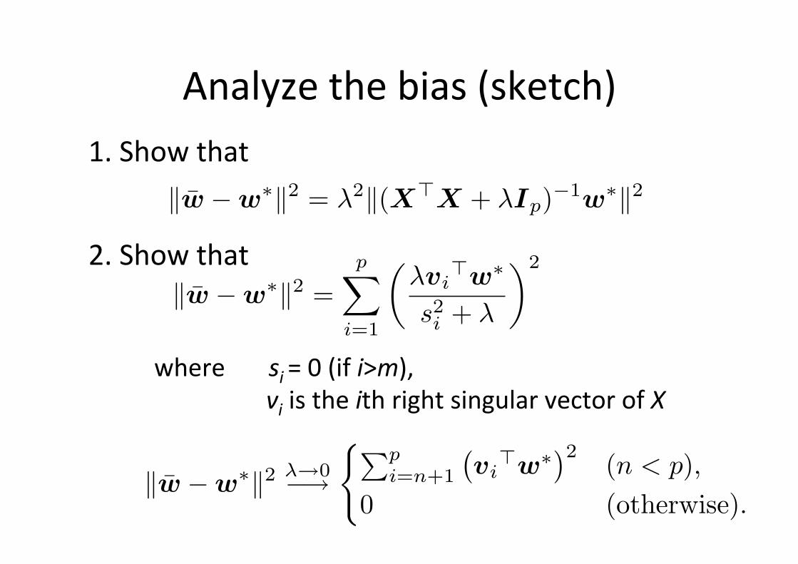
Analyze the bias (sketch) 1. Show that
�w −w∗�2 = λ2�(X�X + λIp)−1w∗�2
2. Show that
where si = 0 (if i>m), vi is the ith right singular vector of X
�w −w∗�2 =p�
i=1
�λvi
�w∗
s2i + λ
�2
�w −w∗�2 λ→0−→��p
i=n+1
�vi�w∗�2 (n < p),
0 (otherwise).
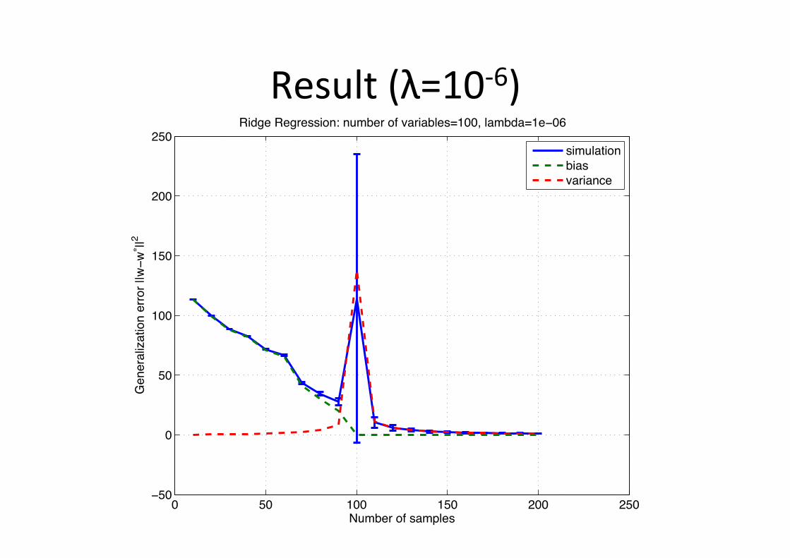
Result (λ=10-‐6)
! "! #!! #"! $!! $"!!"!
!
"!
#!!
#"!
$!!
$"!
%&'()*+,-+./'01).
2)3)*/145/64,3+)**,*+778!8!77$
94:;)+9);*)..4,3<+3&'()*+,-+=/*4/(1).>#!!?+1/'(:/>#)!!@
+
+
.4'&1/64,3
(4/.
=/*4/3A)
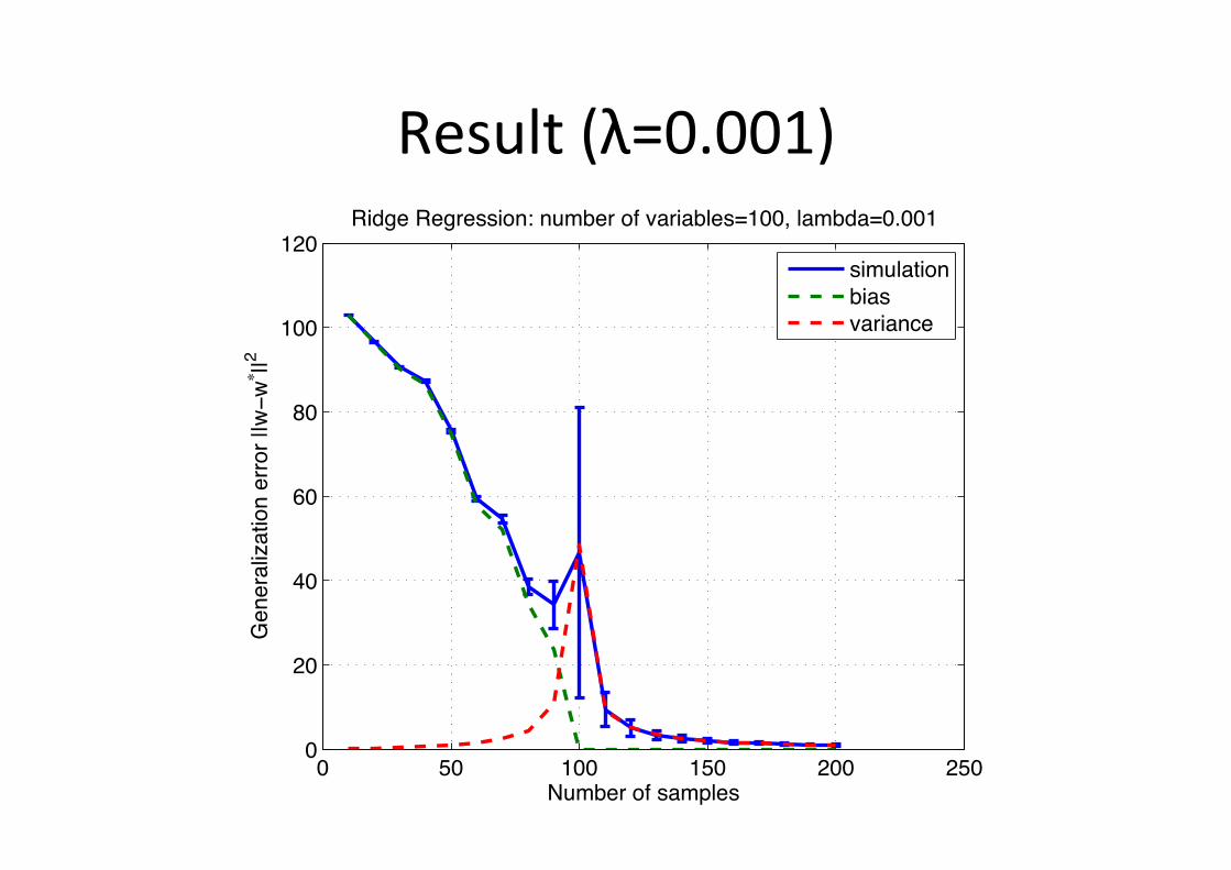
Result (λ=0.001)
! "! #!! #"! $!! $"!!
$!
%!
&!
'!
#!!
#$!
()*+,-./0.12*34,1
5,6,-2478297/6.,--/-.::;!;!::$
<7=>,.<,>-,117/6?.6)*+,-./0.@2-72+4,1A#!!B.42*+=2A!C!!#
.
.
17*)4297/6
+721
@2-726D,

Result (λ=1)
! "! #!! #"! $!! $"!!
$!
%!
&!
'!
#!!
#$!
()*+,-./0.12*34,1
5,6,-2478297/6.,--/-.::;!;!::$
<7=>,.<,>-,117/6?.6)*+,-./0.@2-72+4,1A#!!B.42*+=2A#
.
.
17*)4297/6
+721
@2-726C,
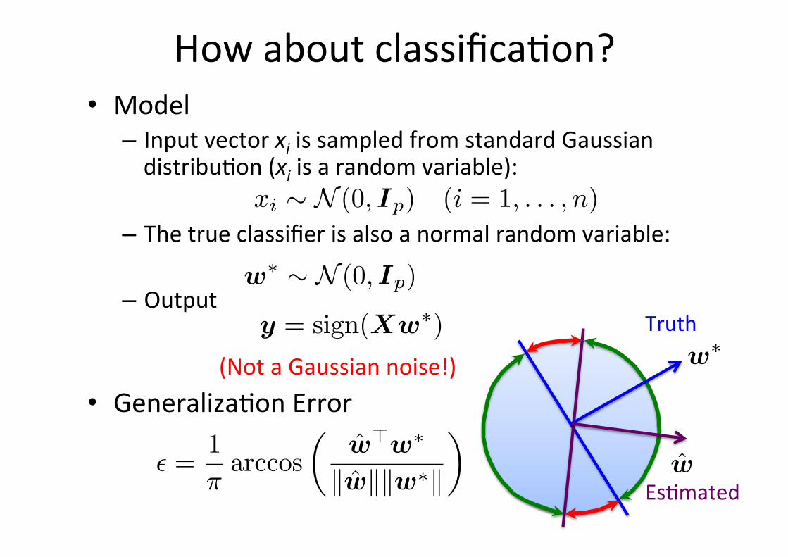
How about classifica6on? • Model – Input vector xi is sampled from standard Gaussian distribu6on (xi is a random variable):
– The true classifier is also a normal random variable:
– Output
(Not a Gaussian noise!) • Generaliza6on Error
y = sign(Xw∗)
Es6mated
Truth
w
w∗
� =1π
arccos�
w�w∗
�w��w∗�
�
xi ∼ N (0, Ip) (i = 1, . . . , n)
w∗ ∼ N (0, Ip)
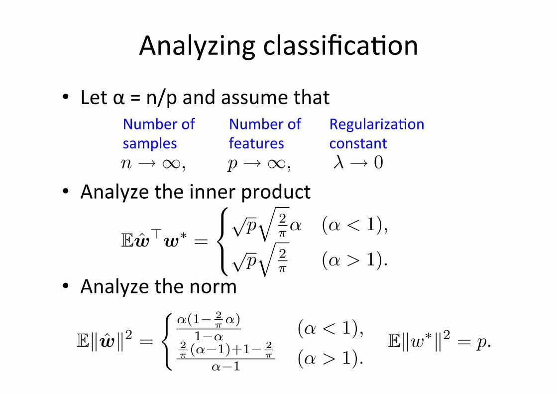
Analyzing classifica6on
• Let α = n/p and assume that
• Analyze the inner product
• Analyze the norm
Number of samples
Number of features
Regulariza6on constant
n→∞, p→∞, λ→ 0
Ew�w∗ =
√p�
2π α (α < 1),
√p�
2π (α > 1).
E�w∗�2 = p.E�w�2 =
�α(1− 2
π α)1−α (α < 1),
2π (α−1)+1− 2
πα−1 (α > 1).
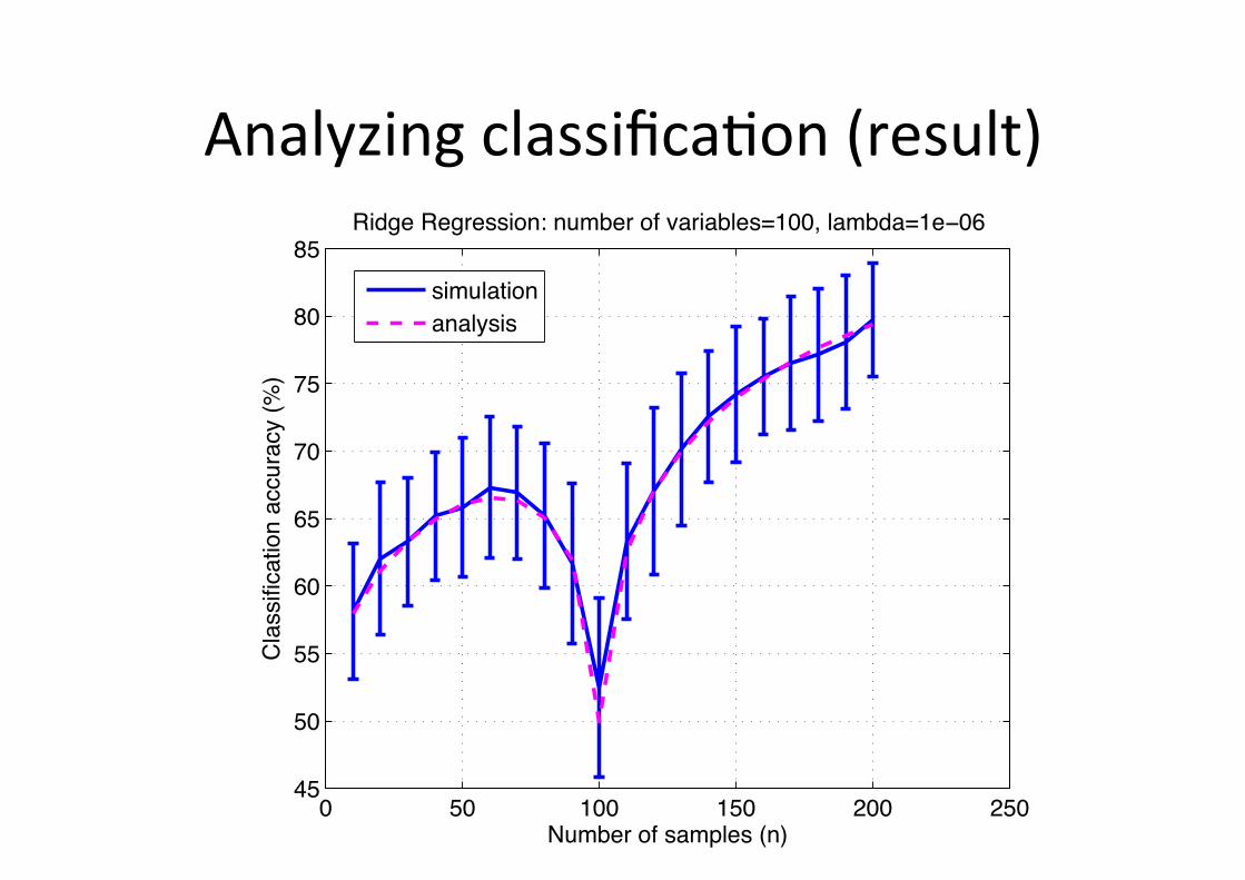
Analyzing classifica6on (result)
! "! #!! #"! $!! $"!%"
"!
""
&!
&"
'!
'"
(!
("
)*+,-./01/23+45-2/678
95322:1:;3<:07/3;;*.3;=/6>8
?:@A-/?-A.-22:07B/7*+,-./01/C3.:3,5-2D#!!E/53+,@3D#-!!&
/
/
2:+*53<:07
3735=2:2
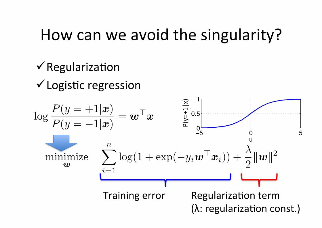
How can we avoid the singularity?
ü Regulariza6on ü Logis6c regression
!! " !"
"#!
$
%
!&'%(
P(y=+1|x)
logP (y = +1|x)P (y = −1|x)
= w�x
minimizew
n�
i=1
log(1 + exp(−yiw�xi)) +
λ
2�w�2
Training error Regulariza6on term (λ: regulariza6on const.)
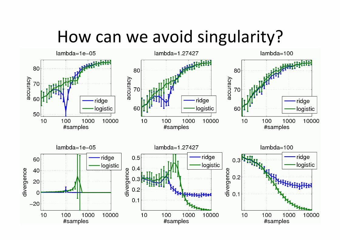
How can we avoid singularity?
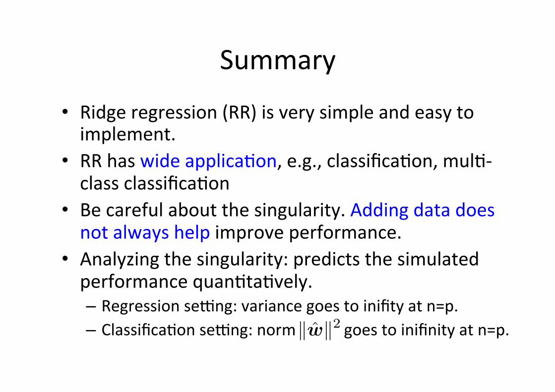
Summary
• Ridge regression (RR) is very simple and easy to implement.
• RR has wide applica6on, e.g., classifica6on, mul6-‐class classifica6on
• Be careful about the singularity. Adding data does not always help improve performance.
• Analyzing the singularity: predicts the simulated performance quan6ta6vely. – Regression segng: variance goes to inifity at n=p. – Classifica6on segng: norm goes to inifinity at n=p. �w�2
Further readings
• Elements of Sta6s6cal Learning (Has6e, Tibshirani, Friedman) 2009 (2nd edi6on) – Ridge regression (Sec. 3.4) – Bias & variance (Sec. 7.3) – Cross valida6on (Sec. 7.10)
• Sta6s6cal Mechanics of Generaliza6on (Opper and Kinzel) in Models of neural networks III: Associa?on, generaliza?on, and representa?on, 1995. – Analysis of perceptron – Singularity