UNIVERSITA’ DEGLI STUDI ROMA TRE DIPARTIMENTO DI … · • μ: coefficiente di attrito...
24
1 UNIVERSITA’ DEGLI STUDI ROMA TRE DIPARTIMENTO DI INGEGNERIA CORSO DI LAUREA IN INGEGNERIA CIVILE PER LA PROTEZIONE Relazione di fine tirocinio “Sviluppo e applicazione di una metodologia di progetto per il rinforzo di volte con materiali FRM” Relatore: Candidato: Prof. Gianmarco de Felice Edoardo Pela Correlatore: Dott. Giovanni Tomaselli Anno Accademico 2017/2018
Transcript of UNIVERSITA’ DEGLI STUDI ROMA TRE DIPARTIMENTO DI … · • μ: coefficiente di attrito...
1
UNIVERSITA’ DEGLI STUDI ROMA TRE
DIPARTIMENTO DI INGEGNERIA CORSO DI LAUREA IN INGEGNERIA CIVILE PER LA
PROTEZIONE
Relazione di fine tirocinio
“Sviluppo e applicazione di una metodologia di progetto per il
rinforzo di volte con materiali FRM”
Relatore: Candidato:
Prof. Gianmarco de Felice Edoardo Pela
Correlatore:
Dott. Giovanni Tomaselli
Anno Accademico 2017/2018
2
Sommario
Premessa .................................................................................................................... 3
Raccolta dati .............................................................................................................. 4
Prove sperimentali ..................................................................................................... 4
Simulazione delle prove: Procedura teorica ............................................................... 7
Calibrazione coefficienti Alfa .................................................................................... 22
3
Premessa
La seguente relazione descrive le attività effettuate ai fini dello svolgimento del tirocinio
formativo, nel periodo tra marzo -giugno 2018.
Il lavoro svolto è stato finalizzato all’apprendimento e all’utilizzo del software di calcolo Matlab
R2018.
La prima fase del tirocinio è stata dedicata all’interpretazione di prove in laboratorio effettuate da
ricercatori della nostra e di altre università sulle volte in muratura rinforzate. Da queste prove
sono stati estrapolati dati relativi alle caratteristiche meccaniche dei materiali, alle caratteristiche
geometriche, nonché i risultati ottenuti a seguito dell’applicazione dei vari sistemi di rinforzo.
Una procedura di calcolo teorica è allora stata implementata sul software di calcolo MatlabR2018
al fine di simulare le prove sperimentali e confrontare i risultati teorici con quelli sperimentali.
Tale procedura di calcolo si è resa inoltre indispensabile al fine di tarare dei coefficienti riguardanti
le deformazioni dei materiali e l’incremento di resistenza dovuto al rinforzo che saranno descritti
in maniera più approfondita di seguito.
4
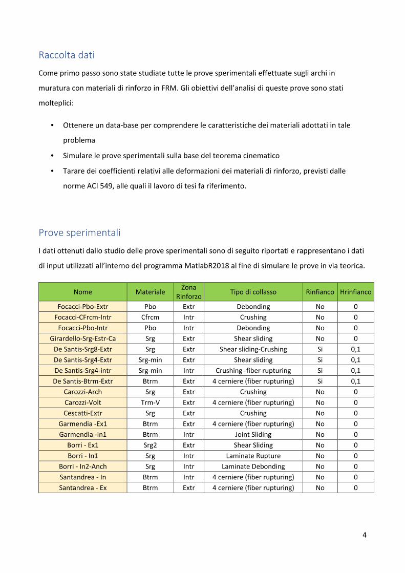
Raccolta dati
Come primo passo sono state studiate tutte le prove sperimentali effettuate sugli archi in
muratura con materiali di rinforzo in FRM. Gli obiettivi dell’analisi di queste prove sono stati
molteplici:
• Ottenere un data-base per comprendere le caratteristiche dei materiali adottati in tale
problema
• Simulare le prove sperimentali sulla base del teorema cinematico
• Tarare dei coefficienti relativi alle deformazioni dei materiali di rinforzo, previsti dalle
norme ACI 549, alle quali il lavoro di tesi fa riferimento.
Prove sperimentali
I dati ottenuti dallo studio delle prove sperimentali sono di seguito riportati e rappresentano i dati
di input utilizzati all’interno del programma MatlabR2018 al fine di simulare le prove in via teorica.
Nome Materiale Zona
Rinforzo Tipo di collasso Rinfianco Hrinfianco
Focacci-Pbo-Extr Pbo Extr Debonding No 0
Focacci-CFrcm-Intr Cfrcm Intr Crushing No 0
Focacci-Pbo-Intr Pbo Intr Debonding No 0
Girardello-Srg-Estr-Ca Srg Extr Shear sliding No 0
De Santis-Srg8-Extr Srg Extr Shear sliding-Crushing Si 0,1
De Santis-Srg4-Extr Srg-min Extr Shear sliding Si 0,1
De Santis-Srg4-intr Srg-min Intr Crushing -fiber rupturing Si 0,1
De Santis-Btrm-Extr Btrm Extr 4 cerniere (fiber rupturing) Si 0,1
Carozzi-Arch Srg Extr Crushing No 0
Carozzi-Volt Trm-V Extr 4 cerniere (fiber rupturing) No 0
Cescatti-Extr Srg Extr Crushing No 0
Garmendia -Ex1 Btrm Extr 4 cerniere (fiber rupturing) No 0
Garmendia -In1 Btrm Intr Joint Sliding No 0
Borri - Ex1 Srg2 Extr Shear Sliding No 0
Borri - In1 Srg Intr Laminate Rupture No 0
Borri - In2-Anch Srg Intr Laminate Debonding No 0
Santandrea - In Btrm Intr 4 cerniere (fiber rupturing) No 0
Santandrea - Ex Btrm Extr 4 cerniere (fiber rupturing) No 0
5
Nome Densità α-in α-fin Ri Re t B
Focacci-Pbo-Extr 20 23,95 156,05 0,866 0,961 0,095 0,095
Focacci-CFrcm-Intr 20 23,95 156,05 0,866 0,961 0,095 0,095
Focacci-Pbo-Intr 20 23,95 156,05 0,866 0,961 0,095 0,095
Girardello-Srg-Estr-Ca 18 24,01 155,99 1,550 1,670 0,120 0,700
De Santis-Srg8-Extr 15,8 48,89 131,11 1,845 1,900 0,055 0,500
De Santis-Srg4-Extr 15,8 48,89 131,11 1,845 1,900 0,055 0,500
De Santis-Srg4-intr 15,8 48,89 131,11 1,845 1,900 0,055 0,500
De Santis-Btrm-Extr 15,8 48,89 131,11 1,845 1,900 0,055 0,500
Carozzi-Arch 18 49,89 130,11 2,030 2,150 0,120 0,250
Carozzi-Volt 18 49,03 130,97 2,030 2,150 0,060 0,300
Cescatti-Extr 18 41,39 138,61 3,608 3,888 0,280 0,800
Garmendia -Ex1 20 30,31 149,69 0,660 0,780 0,120 0,250
Garmendia -In1 20 30,31 149,69 0,660 0,780 0,120 0,250
Borri - Ex1 24 38,81 141,19 1,261 1,361 0,100 0,150
Borri - In1 24 38,81 141,19 1,261 1,361 0,100 0,150
Borri - In2-Anch 24 38,81 141,19 1,261 1,361 0,100 0,150
Santandrea - In 18 41,56 138,44 1,810 1,930 0,120 0,800
Santandrea - Ex 18 41,56 138,44 1,810 1,930 0,120 0,800
Nome fmu Coesione εmu Ef εdb tf Bf
Focacci-Pbo-Extr 8,53 0,200 0,0076 255900 0,00431 0,014 0,095
Focacci-CFrcm-Intr 8,53 0,200 0,0076 242000 0,00471 0,047 0,095
Focacci-Pbo-Intr 8,5 0,200 0,0076 255900 0,00431 0,014 0,095
Girardello-Srg-Estr-Ca 5,97 0,100 0,0054 186000 0,00899 0,084 0,224
De Santis-Srg8-Extr 8 0,200 0,0035 186000 0,00899 0,168 0,150
De Santis-Srg4-Extr 8 0,200 0,0035 186000 0,00899 0,084 0,150
De Santis-Srg4-intr 8 0,200 0,0035 186000 0,00899 0,084 0,150
De Santis-Btrm-Extr 8 0,200 0,0035 52100 0,0121 0,064 0,500
Carozzi-Arch 3,5 0,200 0,0076 186000 0,00899 0,102 0,250
Carozzi-Volt 3,5 0,200 0,0076 72000 0,00427 0,048 0,250
Cescatti-Extr 3 0,200 0,0035 186000 0,00899 0,084 0,250
Garmendia -Ex1 5,6 0,200 0,0035 52100 0,0121 0,042 0,250
Garmendia -In1 5,6 0,200 0,0035 52100 0,0121 0,042 0,250
Borri - Ex1 15,3 0,100 0,0076 160000 0,00899 0,383 0,150
Borri - In1 15,3 0,100 0,0076 186000 0,00899 0,098 0,150
Borri - In2-Anch 15,3 0,100 0,0076 186000 0,00899 0,098 0,150
Santandrea - In 9 0,200 0,0035 70000 0,0121 0,032 0,400
Santandrea - Ex 9 0,200 0,0035 70000 0,0121 0,032 0,400
6
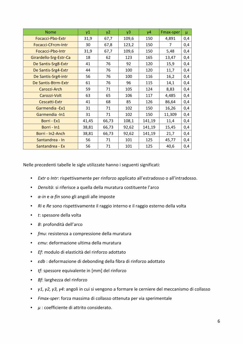
Nome γ1 γ2 γ3 γ4 Fmax-sper μ
Focacci-Pbo-Extr 31,9 67,7 109,6 150 4,891 0,4
Focacci-CFrcm-Intr 30 67,8 123,2 150 7 0,4
Focacci-Pbo-Intr 31,9 67,7 109,6 150 5,48 0,4
Girardello-Srg-Estr-Ca 18 62 123 165 13,47 0,4
De Santis-Srg8-Extr 41 76 92 120 15,9 0,4
De Santis-Srg4-Extr 44 76 100 120 11,7 0,4
De Santis-Srg4-intr 56 76 100 116 16,2 0,4
De Santis-Btrm-Extr 61 76 96 115 14,1 0,4
Carozzi-Arch 59 71 105 124 8,83 0,4
Carozzi-Volt 63 65 106 117 4,485 0,4
Cescatti-Extr 41 68 85 126 86,64 0,4
Garmendia -Ex1 31 71 102 150 16,26 0,4
Garmendia -In1 31 71 102 150 11,309 0,4
Borri - Ex1 41,45 66,73 108,1 141,19 11,4 0,4
Borri - In1 38,81 66,73 92,62 141,19 15,45 0,4
Borri - In2-Anch 38,81 66,73 92,62 141,19 21,7 0,4
Santandrea - In 56 71 101 125 45,77 0,4
Santandrea - Ex 56 71 101 125 40,6 0,4
Nelle precedenti tabelle le sigle utilizzate hanno i seguenti significati:
• Extr o Intr: rispettivamente per rinforzo applicato all’estradosso o all’intradosso.
• Densità: si riferisce a quella della muratura costituente l’arco
• α-in e α-fin sono gli angoli alle imposte
• Ri e Re sono rispettivamente il raggio interno e il raggio esterno della volta
• t: spessore della volta
• B: profondità dell’arco
• fmu: resistenza a compressione della muratura
• εmu: deformazione ultima della muratura
• Ef: modulo di elasticità del rinforzo adottato
• εdb : deformazione di debonding della fibra di rinforzo adottato
• tf: spessore equivalente in [mm] del rinforzo
• Bf: larghezza del rinforzo
• γ1, γ2, γ3, γ4: angoli in cui si vengono a formare le cerniere del meccanismo di collasso
• Fmax-sper: forza massima di collasso ottenuta per via sperimentale
• μ : coefficiente di attrito considerato.
7
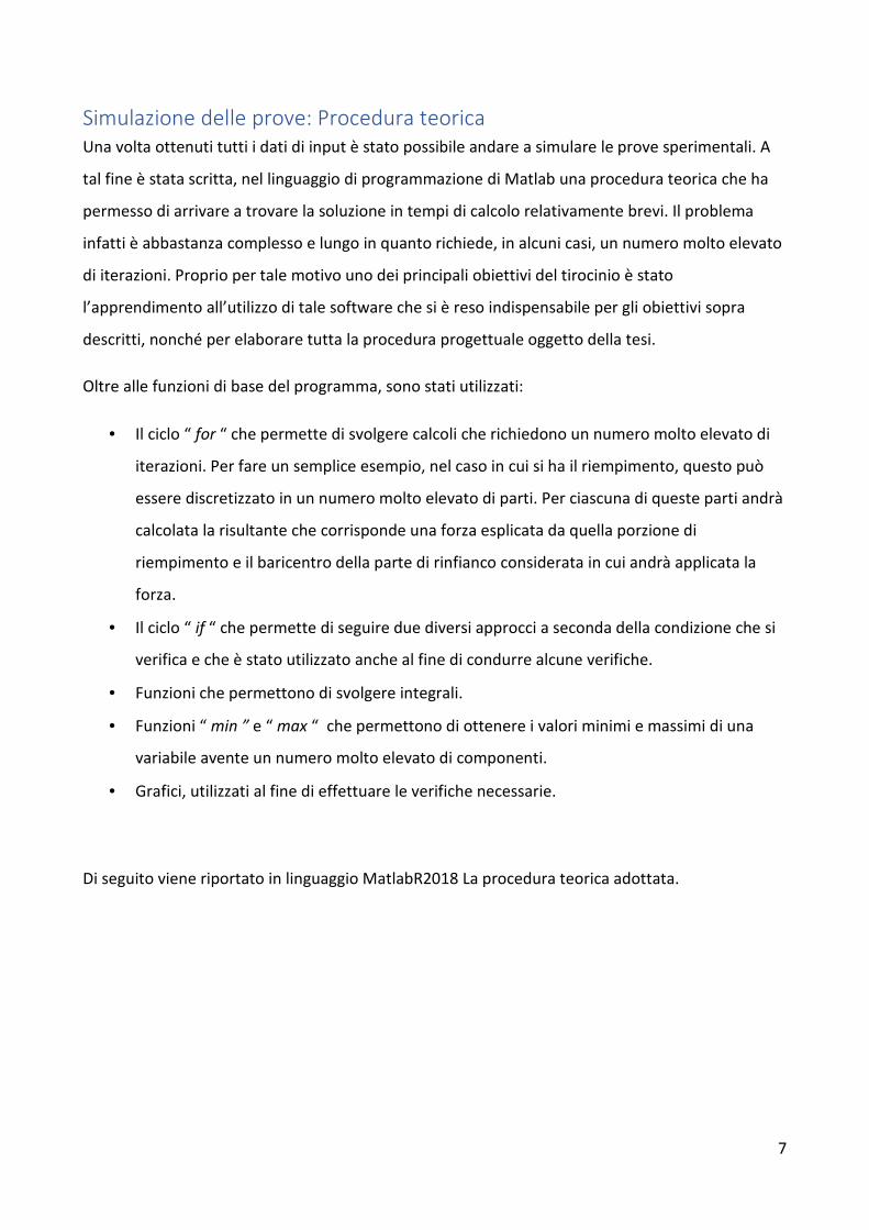
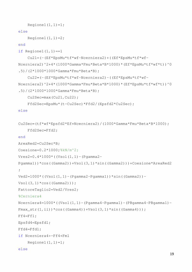
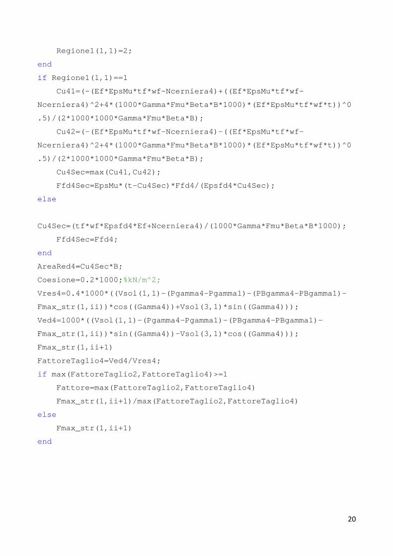
Simulazione delle prove: Procedura teorica
Una volta ottenuti tutti i dati di input è stato possibile andare a simulare le prove sperimentali. A
tal fine è stata scritta, nel linguaggio di programmazione di Matlab una procedura teorica che ha
permesso di arrivare a trovare la soluzione in tempi di calcolo relativamente brevi. Il problema
infatti è abbastanza complesso e lungo in quanto richiede, in alcuni casi, un numero molto elevato
di iterazioni. Proprio per tale motivo uno dei principali obiettivi del tirocinio è stato
l’apprendimento all’utilizzo di tale software che si è reso indispensabile per gli obiettivi sopra
descritti, nonché per elaborare tutta la procedura progettuale oggetto della tesi.
Oltre alle funzioni di base del programma, sono stati utilizzati:
• Il ciclo “ for “ che permette di svolgere calcoli che richiedono un numero molto elevato di
iterazioni. Per fare un semplice esempio, nel caso in cui si ha il riempimento, questo può
essere discretizzato in un numero molto elevato di parti. Per ciascuna di queste parti andrà
calcolata la risultante che corrisponde una forza esplicata da quella porzione di
riempimento e il baricentro della parte di rinfianco considerata in cui andrà applicata la
forza.
• Il ciclo “ if “ che permette di seguire due diversi approcci a seconda della condizione che si
verifica e che è stato utilizzato anche al fine di condurre alcune verifiche.
• Funzioni che permettono di svolgere integrali.
• Funzioni “ min ” e “ max “ che permettono di ottenere i valori minimi e massimi di una
variabile avente un numero molto elevato di componenti.
• Grafici, utilizzati al fine di effettuare le verifiche necessarie.
Di seguito viene riportato in linguaggio MatlabR2018 La procedura teorica adottata.
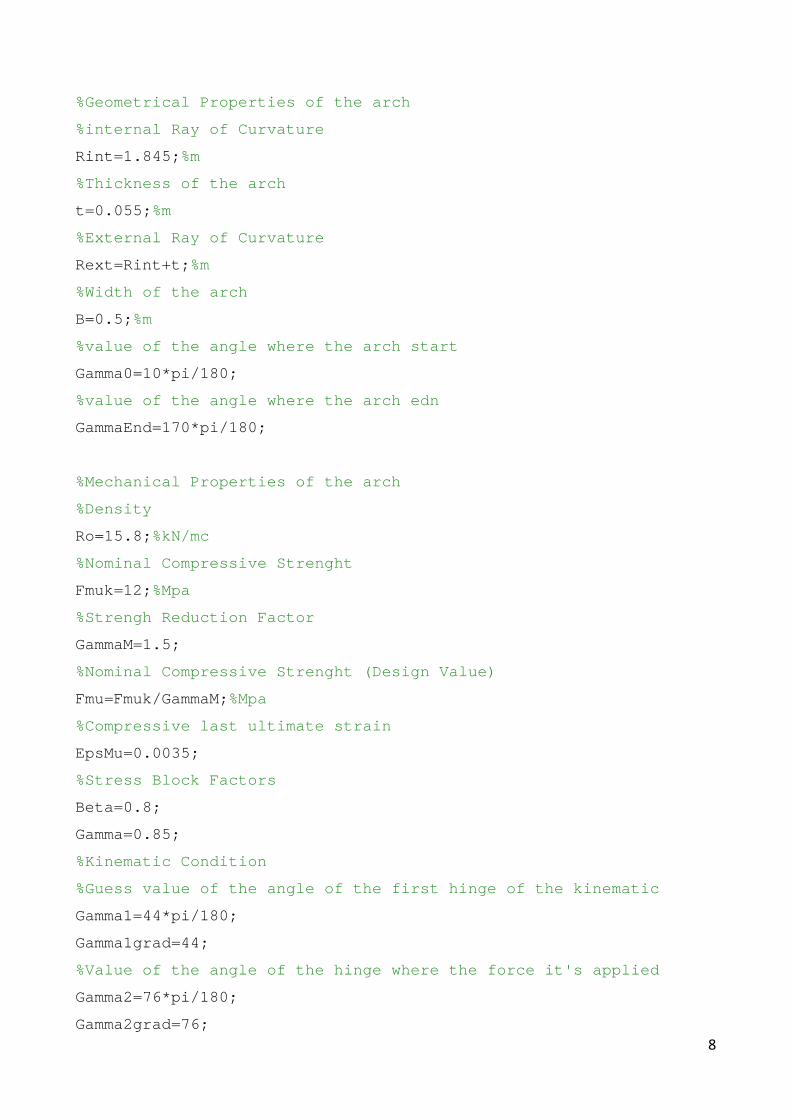
8
%Geometrical Properties of the arch
%internal Ray of Curvature
Rint=1.845; %m
%Thickness of the arch
t=0.055; %m
%External Ray of Curvature
Rext=Rint+t; %m
%Width of the arch
B=0.5; %m
%value of the angle where the arch start
Gamma0=10*pi/180;
%value of the angle where the arch edn
GammaEnd=170*pi/180;
%Mechanical Properties of the arch
%Density
Ro=15.8; %kN/mc
%Nominal Compressive Strenght
Fmuk=12; %Mpa
%Strengh Reduction Factor
GammaM=1.5;
%Nominal Compressive Strenght (Design Value)
Fmu=Fmuk/GammaM;%Mpa
%Compressive last ultimate strain
EpsMu=0.0035;
%Stress Block Factors
Beta=0.8;
Gamma=0.85;
%Kinematic Condition
%Guess value of the angle of the first hinge of the kinematic
Gamma1=44*pi/180;
Gamma1grad=44;
%Value of the angle of the hinge where the force it 's applied
Gamma2=76*pi/180;
Gamma2grad=76;
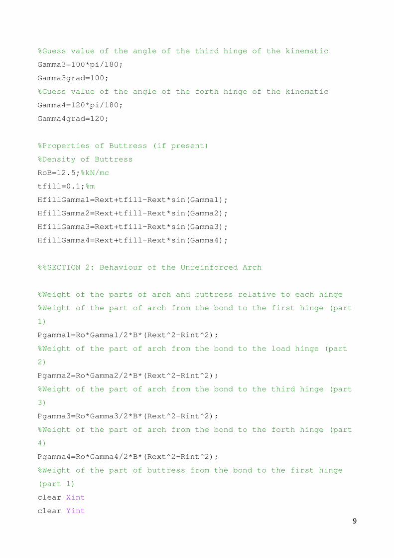
9
%Guess value of the angle of the third hinge of the kinematic
Gamma3=100*pi/180;
Gamma3grad=100;
%Guess value of the angle of the forth hinge of the kinematic
Gamma4=120*pi/180;
Gamma4grad=120;
%Properties of Buttress (if present)
%Density of Buttress
RoB=12.5; %kN/mc
tfill=0.1; %m
HfillGamma1=Rext+tfill-Rext*sin(Gamma1);
HfillGamma2=Rext+tfill-Rext*sin(Gamma2);
HfillGamma3=Rext+tfill-Rext*sin(Gamma3);
HfillGamma4=Rext+tfill-Rext*sin(Gamma4);
%%SECTION 2: Behaviour of the Unreinforced Arch
%Weight of the parts of arch and buttress relative to each hinge
%Weight of the part of arch from the bond to the fi rst hinge (part
1)
Pgamma1=Ro*Gamma1/2*B*(Rext^2-Rint^2);
%Weight of the part of arch from the bond to the lo ad hinge (part
2)
Pgamma2=Ro*Gamma2/2*B*(Rext^2-Rint^2);
%Weight of the part of arch from the bond to the th ird hinge (part
3)
Pgamma3=Ro*Gamma3/2*B*(Rext^2-Rint^2);
%Weight of the part of arch from the bond to the fo rth hinge (part
4)
Pgamma4=Ro*Gamma4/2*B*(Rext^2-Rint^2);
%Weight of the part of buttress from the bond to th e first hinge
(part 1)
clear Xint
clear Yint
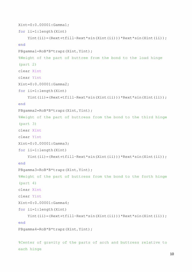
10
Xint=0:0.00001:Gamma1;
for ii=1:length(Xint)
Yint(ii)=(Rext+tfill-Rext*sin(Xint(ii)))*Rext*s in(Xint(ii));
end
PBgamma1=RoB*B*trapz(Xint,Yint);
%Weight of the part of buttree from the bond to the load hinge
(part 2)
clear Xint
clear Yint
Xint=0:0.00001:Gamma2;
for ii=1:length(Xint)
Yint(ii)=(Rext+tfill-Rext*sin(Xint(ii)))*Rext*s in(Xint(ii));
end
PBgamma2=RoB*B*trapz(Xint,Yint);
%Weight of the part of buttress from the bond to th e third hinge
(part 3)
clear Xint
clear Yint
Xint=0:0.00001:Gamma3;
for ii=1:length(Xint)
Yint(ii)=(Rext+tfill-Rext*sin(Xint(ii)))*Rext*s in(Xint(ii));
end
PBgamma3=RoB*B*trapz(Xint,Yint);
%Weight of the part of buttress from the bond to th e forth hinge
(part 4)
clear Xint
clear Yint
Xint=0:0.00001:Gamma4;
for ii=1:length(Xint)
Yint(ii)=(Rext+tfill-Rext*sin(Xint(ii)))*Rext*s in(Xint(ii));
end
PBgamma4=RoB*B*trapz(Xint,Yint);
%Center of gravity of the parts of arch and buttres s relative to
each hinge
11
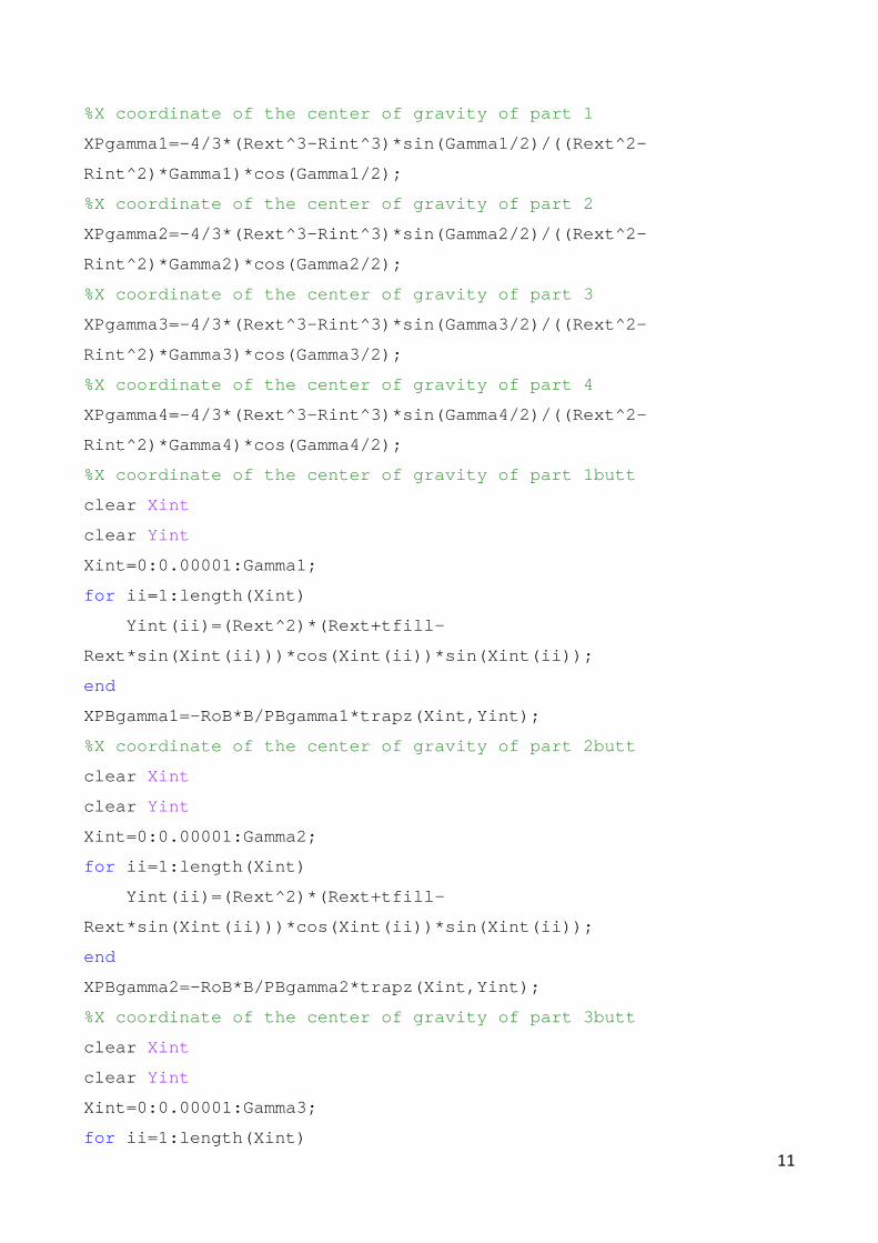
%X coordinate of the center of gravity of part 1
XPgamma1=-4/3*(Rext^3-Rint^3)*sin(Gamma1/2)/((Rext^ 2-
Rint^2)*Gamma1)*cos(Gamma1/2);
%X coordinate of the center of gravity of part 2
XPgamma2=-4/3*(Rext^3-Rint^3)*sin(Gamma2/2)/((Rext^ 2-
Rint^2)*Gamma2)*cos(Gamma2/2);
%X coordinate of the center of gravity of part 3
XPgamma3=-4/3*(Rext^3-Rint^3)*sin(Gamma3/2)/((Rext^ 2-
Rint^2)*Gamma3)*cos(Gamma3/2);
%X coordinate of the center of gravity of part 4
XPgamma4=-4/3*(Rext^3-Rint^3)*sin(Gamma4/2)/((Rext^ 2-
Rint^2)*Gamma4)*cos(Gamma4/2);
%X coordinate of the center of gravity of part 1but t
clear Xint
clear Yint
Xint=0:0.00001:Gamma1;
for ii=1:length(Xint)
Yint(ii)=(Rext^2)*(Rext+tfill-
Rext*sin(Xint(ii)))*cos(Xint(ii))*sin(Xint(ii));
end
XPBgamma1=-RoB*B/PBgamma1*trapz(Xint,Yint);
%X coordinate of the center of gravity of part 2but t
clear Xint
clear Yint
Xint=0:0.00001:Gamma2;
for ii=1:length(Xint)
Yint(ii)=(Rext^2)*(Rext+tfill-
Rext*sin(Xint(ii)))*cos(Xint(ii))*sin(Xint(ii));
end
XPBgamma2=-RoB*B/PBgamma2*trapz(Xint,Yint);
%X coordinate of the center of gravity of part 3but t
clear Xint
clear Yint
Xint=0:0.00001:Gamma3;
for ii=1:length(Xint)
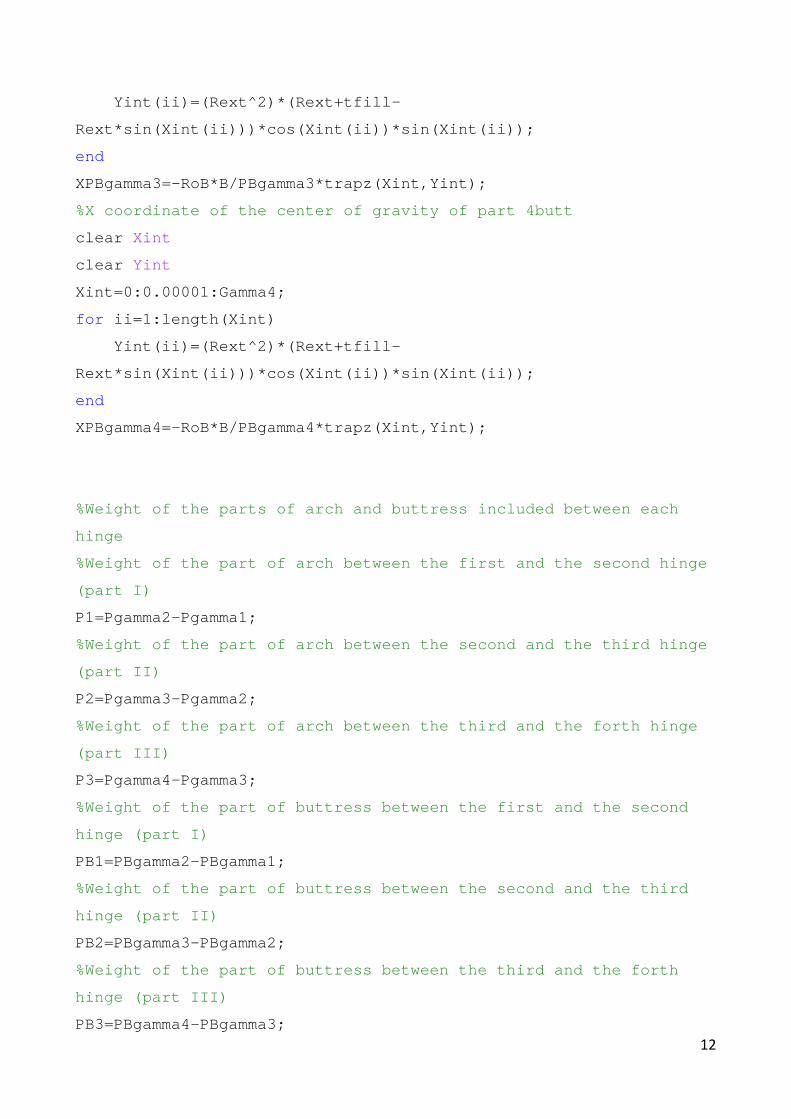
12
Yint(ii)=(Rext^2)*(Rext+tfill-
Rext*sin(Xint(ii)))*cos(Xint(ii))*sin(Xint(ii));
end
XPBgamma3=-RoB*B/PBgamma3*trapz(Xint,Yint);
%X coordinate of the center of gravity of part 4but t
clear Xint
clear Yint
Xint=0:0.00001:Gamma4;
for ii=1:length(Xint)
Yint(ii)=(Rext^2)*(Rext+tfill-
Rext*sin(Xint(ii)))*cos(Xint(ii))*sin(Xint(ii));
end
XPBgamma4=-RoB*B/PBgamma4*trapz(Xint,Yint);
%Weight of the parts of arch and buttress included between each
hinge
%Weight of the part of arch between the first and t he second hinge
(part I)
P1=Pgamma2-Pgamma1;
%Weight of the part of arch between the second and the third hinge
(part II)
P2=Pgamma3-Pgamma2;
%Weight of the part of arch between the third and t he forth hinge
(part III)
P3=Pgamma4-Pgamma3;
%Weight of the part of buttress between the first a nd the second
hinge (part I)
PB1=PBgamma2-PBgamma1;
%Weight of the part of buttress between the second and the third
hinge (part II)
PB2=PBgamma3-PBgamma2;
%Weight of the part of buttress between the third a nd the forth
hinge (part III)
PB3=PBgamma4-PBgamma3;
13
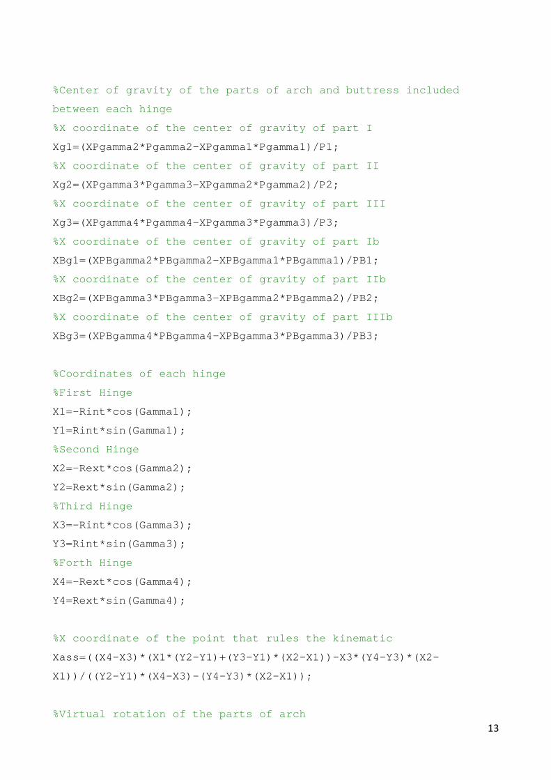
%Center of gravity of the parts of arch and buttres s included
between each hinge
%X coordinate of the center of gravity of part I
Xg1=(XPgamma2*Pgamma2-XPgamma1*Pgamma1)/P1;
%X coordinate of the center of gravity of part II
Xg2=(XPgamma3*Pgamma3-XPgamma2*Pgamma2)/P2;
%X coordinate of the center of gravity of part III
Xg3=(XPgamma4*Pgamma4-XPgamma3*Pgamma3)/P3;
%X coordinate of the center of gravity of part Ib
XBg1=(XPBgamma2*PBgamma2-XPBgamma1*PBgamma1)/PB1;
%X coordinate of the center of gravity of part IIb
XBg2=(XPBgamma3*PBgamma3-XPBgamma2*PBgamma2)/PB2;
%X coordinate of the center of gravity of part IIIb
XBg3=(XPBgamma4*PBgamma4-XPBgamma3*PBgamma3)/PB3;
%Coordinates of each hinge
%First Hinge
X1=-Rint*cos(Gamma1);
Y1=Rint*sin(Gamma1);
%Second Hinge
X2=-Rext*cos(Gamma2);
Y2=Rext*sin(Gamma2);
%Third Hinge
X3=-Rint*cos(Gamma3);
Y3=Rint*sin(Gamma3);
%Forth Hinge
X4=-Rext*cos(Gamma4);
Y4=Rext*sin(Gamma4);
%X coordinate of the point that rules the kinematic
Xass=((X4-X3)*(X1*(Y2-Y1)+(Y3-Y1)*(X2-X1))-X3*(Y4-Y 3)*(X2-
X1))/((Y2-Y1)*(X4-X3)-(Y4-Y3)*(X2-X1));
%Virtual rotation of the parts of arch
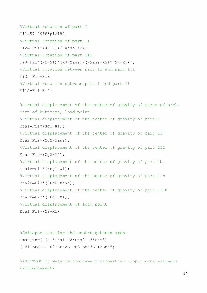
14
%Virtual rotation of part I
Fi1=57.2958*pi/180;
%Virtual rotation of part II
Fi2=-Fi1*(X2-X1)/(Xass-X2);
%Virtual rotation of part III
Fi3=Fi1*(X2-X1)*(X3-Xass)/((Xass-X2)*(X4-X3));
%Virtual rotation between part II and part III
Fi23=Fi3-Fi2;
%Virtual rotation between part I and part II
Fi12=Fi1-Fi2;
%Virtual displacement of the center of gravity of p arts of arch,
part of buttress, load point
%Virtual displacement of the center of gravity of p art I
Eta1=Fi1*(Xg1-X1);
%Virtual displacement of the center of gravity of p art II
Eta2=Fi2*(Xg2-Xass);
%Virtual displacement of the center of gravity of p art III
Eta3=Fi3*(Xg3-X4);
%Virtual displacement of the center of gravity of p art Ib
Eta1B=Fi1*(XBg1-X1);
%Virtual displacement of the center of gravity of p art IIb
Eta2B=Fi2*(XBg2-Xass);
%Virtual displacement of the center of gravity of p art IIIb
Eta3B=Fi3*(XBg3-X4);
%Virtual displacement of load point
Etaf=Fi1*(X2-X1);
%Collapse load for the unstrenghtened arch
Fmax_un=(-(P1*Eta1+P2*Eta2+P3*Eta3)-
(PB1*Eta1B+PB2*Eta2B+PB3*Eta3B))/Etaf;
%%SECTION 3: Mesh reinforcement properties (input d ata-extrados
reinforcement)
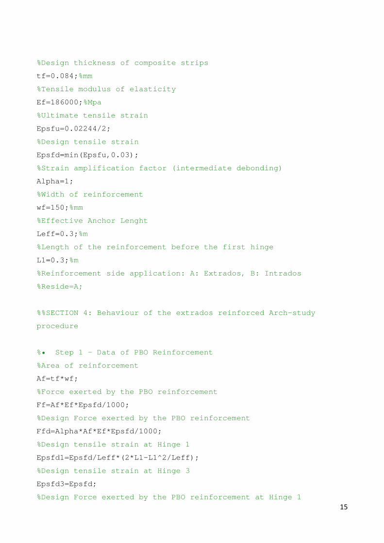
15
%Design thickness of composite strips
tf=0.084; %mm
%Tensile modulus of elasticity
Ef=186000; %Mpa
%Ultimate tensile strain
Epsfu=0.02244/2;
%Design tensile strain
Epsfd=min(Epsfu,0.03);
%Strain amplification factor (intermediate debondin g)
Alpha=1;
%Width of reinforcement
wf=150; %mm
%Effective Anchor Lenght
Leff=0.3; %m
%Length of the reinforcement before the first hinge
L1=0.3; %m
%Reinforcement side application: A: Extrados, B: In trados
%Reside=A;
%%SECTION 4: Behaviour of the extrados reinforced A rch-study
procedure
%• Step 1 - Data of PBO Reinforcement
%Area of reinforcement
Af=tf*wf;
%Force exerted by the PBO reinforcement
Ff=Af*Ef*Epsfd/1000;
%Design Force exerted by the PBO reinforcement
Ffd=Alpha*Af*Ef*Epsfd/1000;
%Design tensile strain at Hinge 1
Epsfd1=Epsfd/Leff*(2*L1-L1^2/Leff);
%Design tensile strain at Hinge 3
Epsfd3=Epsfd;
%Design Force exerted by the PBO reinforcement at H inge 1
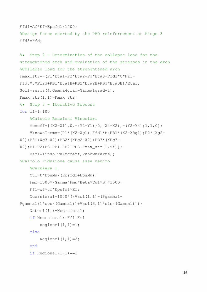
16
Ffd1=Af*Ef*Epsfd1/1000;
%Design Force exerted by the PBO reinforcement at H inge 3
Ffd3=Ffd;
%• Step 2 - Determination of the collapse load for the
strenghtened arch and evaluation of the stresses in the arch
%Collapse load for the strenghtened arch
Fmax_str=-(P1*Eta1+P2*Eta2+P3*Eta3-Ffd1*t*Fi1-
Ffd3*t*Fi23+PB1*Eta1B+PB2*Eta2B+PB3*Eta3B)/Etaf;
Soll=zeros(4,Gamma4grad-Gamma1grad+1);
Fmax_str(1,1)=Fmax_str;
%• Step 3 - Iterative Process
for ii=1:100
%Calcolo Reazioni Vincolari
Mcoeff=[(X2-X1),0,-(Y2-Y1);0,(X4-X2),-(Y2-Y4);1 ,1,0];
VknownTerms=[P1*(X2-Xg1)+Ffd1*t+PB1*(X2-XBg1);P 2*(Xg2-
X2)+P3*(Xg3-X2)+PB2*(XBg2-X2)+PB3*(XBg3-
X2);P1+P2+P3+PB1+PB2+PB3+Fmax_str(1,ii)];
Vsol=linsolve(Mcoeff,VknownTerms);
%Calcolo riduzione causa asse neutro
%Cerniera 1
Cu1=t*EpsMu/(Epsfd1+EpsMu);
Fm1=1000*(Gamma*Fmu*Beta*Cu1*B)*1000;
Ff1=wf*tf*Epsfd1*Ef;
Ncerniera1=1000*((Vsol(1,1)-(Pgamma1-
Pgamma1))*cos((Gamma1))+Vsol(3,1)*sin((Gamma1)));
Nstor1(ii)=Ncerniera1;
if Ncerniera1>-Ff1+Fm1
Regione1(1,1)=1;
else
Regione1(1,1)=2;
end
if Regione1(1,1)==1
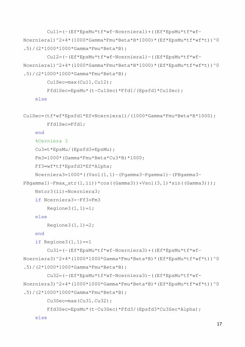
17
Cu11=(-(Ef*EpsMu*tf*wf-Ncerniera1)+((Ef*Eps Mu*tf*wf-
Ncerniera1)^2+4*(1000*Gamma*Fmu*Beta*B*1000)*(Ef*Ep sMu*tf*wf*t))^0
.5)/(2*1000*1000*Gamma*Fmu*Beta*B);
Cu12=(-(Ef*EpsMu*tf*wf-Ncerniera1)-((Ef*Eps Mu*tf*wf-
Ncerniera1)^2+4*(1000*Gamma*Fmu*Beta*B*1000)*(Ef*Ep sMu*tf*wf*t))^0
.5)/(2*1000*1000*Gamma*Fmu*Beta*B);
Cu1Sec=max(Cu11,Cu12);
Ffd1Sec=EpsMu*(t-Cu1Sec)*Ffd1/(Epsfd1*Cu1Se c);
else
Cu1Sec=(tf*wf*Epsfd1*Ef+Ncerniera1)/(1000*Gamma*Fmu *Beta*B*1000);
Ffd1Sec=Ffd1;
end
%Cerniera 3
Cu3=t*EpsMu/(Epsfd3+EpsMu);
Fm3=1000*(Gamma*Fmu*Beta*Cu3*B)*1000;
Ff3=wf*tf*Epsfd3*Ef*Alpha;
Ncerniera3=1000*((Vsol(1,1)-(Pgamma3-Pgamma1)-( PBgamma3-
PBgamma1)-Fmax_str(1,ii))*cos((Gamma3))+Vsol(3,1)*s in((Gamma3)));
Nstor3(ii)=Ncerniera3;
if Ncerniera3>-Ff3+Fm3
Regione3(1,1)=1;
else
Regione3(1,1)=2;
end
if Regione3(1,1)==1
Cu31=(-(Ef*EpsMu*tf*wf-Ncerniera3)+((Ef*Eps Mu*tf*wf-
Ncerniera3)^2+4*(1000*1000*Gamma*Fmu*Beta*B)*(Ef*Ep sMu*tf*wf*t))^0
.5)/(2*1000*1000*Gamma*Fmu*Beta*B);
Cu32=(-(Ef*EpsMu*tf*wf-Ncerniera3)-((Ef*Eps Mu*tf*wf-
Ncerniera3)^2+4*(1000*1000*Gamma*Fmu*Beta*B)*(Ef*Ep sMu*tf*wf*t))^0
.5)/(2*1000*1000*Gamma*Fmu*Beta*B);
Cu3Sec=max(Cu31,Cu32);
Ffd3Sec=EpsMu*(t-Cu3Sec)*Ffd3/(Epsfd3*Cu3Se c*Alpha);
else
18
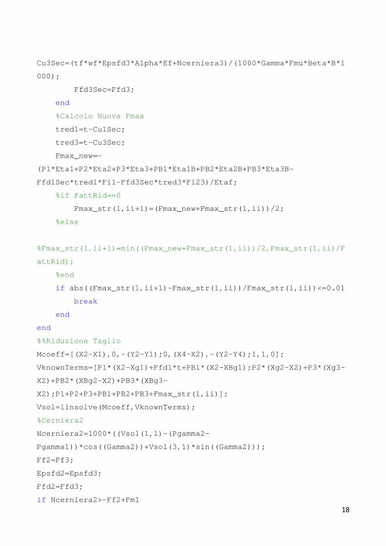
Cu3Sec=(tf*wf*Epsfd3*Alpha*Ef+Ncerniera3)/(1000*Gam ma*Fmu*Beta*B*1
000);
Ffd3Sec=Ffd3;
end
%Calcolo Nuova Fmax
tred1=t-Cu1Sec;
tred3=t-Cu3Sec;
Fmax_new=-
(P1*Eta1+P2*Eta2+P3*Eta3+PB1*Eta1B+PB2*Eta2B+PB3*Et a3B-
Ffd1Sec*tred1*Fi1-Ffd3Sec*tred3*Fi23)/Etaf;
%if FattRid==0
Fmax_str(1,ii+1)=(Fmax_new+Fmax_str(1,ii))/ 2;
%else
%Fmax_str(1,ii+1)=min((Fmax_new+Fmax_str(1,ii))/2,F max_str(1,ii)/F
attRid);
%end
if abs((Fmax_str(1,ii+1)-Fmax_str(1,ii))/Fmax_str(1,i i))<=0.01
break
end
end
%%Riduzione Taglio
Mcoeff=[(X2-X1),0,-(Y2-Y1);0,(X4-X2),-(Y2-Y4);1,1,0 ];
VknownTerms=[P1*(X2-Xg1)+Ffd1*t+PB1*(X2-XBg1);P2*(X g2-X2)+P3*(Xg3-
X2)+PB2*(XBg2-X2)+PB3*(XBg3-
X2);P1+P2+P3+PB1+PB2+PB3+Fmax_str(1,ii)];
Vsol=linsolve(Mcoeff,VknownTerms);
%Cerniera2
Ncerniera2=1000*((Vsol(1,1)-(Pgamma2-
Pgamma1))*cos((Gamma2))+Vsol(3,1)*sin((Gamma2)));
Ff2=Ff3;
Epsfd2=Epsfd3;
Ffd2=Ffd3;
if Ncerniera2>-Ff2+Fm1
19
Regione1(1,1)=1;
else
Regione1(1,1)=2;
end
if Regione1(1,1)==1
Cu21=(-(Ef*EpsMu*tf*wf-Ncerniera2)+((Ef*EpsMu*t f*wf-
Ncerniera2)^2+4*(1000*Gamma*Fmu*Beta*B*1000)*(Ef*Ep sMu*tf*wf*t))^0
.5)/(2*1000*1000*Gamma*Fmu*Beta*B);
Cu22=(-(Ef*EpsMu*tf*wf-Ncerniera2)-((Ef*EpsMu*t f*wf-
Ncerniera2)^2+4*(1000*Gamma*Fmu*Beta*B*1000)*(Ef*Ep sMu*tf*wf*t))^0
.5)/(2*1000*1000*Gamma*Fmu*Beta*B);
Cu2Sec=max(Cu21,Cu22);
Ffd2Sec=EpsMu*(t-Cu2Sec)*Ffd2/(Epsfd2*Cu2Sec);
else
Cu2Sec=(tf*wf*Epsfd2*Ef+Ncerniera2)/(1000*Gamma*Fmu *Beta*B*1000);
Ffd2Sec=Ffd2;
end
AreaRed2=Cu2Sec*B;
Coesione=0.2*1000; %kN/m^2;
Vres2=0.4*1000*((Vsol(1,1)-(Pgamma2-
Pgamma1))*cos((Gamma2))+Vsol(3,1)*sin((Gamma2)))+Co esione*AreaRed2
;
Ved2=1000*((Vsol(1,1)-(Pgamma2-Pgamma1))*sin((Gamma 2))-
Vsol(3,1)*cos((Gamma2)));
FattoreTaglio2=Ved2/Vres2;
%Cerniera4
Ncerniera4=1000*((Vsol(1,1)-(Pgamma4-Pgamma1)-(PBga mma4-PBgamma1)-
Fmax_str(1,ii))*cos((Gamma4))+Vsol(3,1)*sin((Gamma4 )));
Ff4=Ff1;
Epsfd4=Epsfd1;
Ffd4=Ffd1;
if Ncerniera4>-Ff4+Fm1
Regione1(1,1)=1;
else
20
Regione1(1,1)=2;
end
if Regione1(1,1)==1
Cu41=(-(Ef*EpsMu*tf*wf-Ncerniera4)+((Ef*EpsMu*t f*wf-
Ncerniera4)^2+4*(1000*Gamma*Fmu*Beta*B*1000)*(Ef*Ep sMu*tf*wf*t))^0
.5)/(2*1000*1000*Gamma*Fmu*Beta*B);
Cu42=(-(Ef*EpsMu*tf*wf-Ncerniera4)-((Ef*EpsMu*t f*wf-
Ncerniera4)^2+4*(1000*Gamma*Fmu*Beta*B*1000)*(Ef*Ep sMu*tf*wf*t))^0
.5)/(2*1000*1000*Gamma*Fmu*Beta*B);
Cu4Sec=max(Cu41,Cu42);
Ffd4Sec=EpsMu*(t-Cu4Sec)*Ffd4/(Epsfd4*Cu4Sec);
else
Cu4Sec=(tf*wf*Epsfd4*Ef+Ncerniera4)/(1000*Gamma*Fmu *Beta*B*1000);
Ffd4Sec=Ffd4;
end
AreaRed4=Cu4Sec*B;
Coesione=0.2*1000; %kN/m^2;
Vres4=0.4*1000*((Vsol(1,1)-(Pgamma4-Pgamma1)-(PBgam ma4-PBgamma1)-
Fmax_str(1,ii))*cos((Gamma4))+Vsol(3,1)*sin((Gamma4 )));
Ved4=1000*((Vsol(1,1)-(Pgamma4-Pgamma1)-(PBgamma4-P Bgamma1)-
Fmax_str(1,ii))*sin((Gamma4))-Vsol(3,1)*cos((Gamma4 )));
Fmax_str(1,ii+1)
FattoreTaglio4=Ved4/Vres4;
if max(FattoreTaglio2,FattoreTaglio4)>=1
Fattore=max(FattoreTaglio2,FattoreTaglio4)
Fmax_str(1,ii+1)/max(FattoreTaglio2,FattoreTagl io4)
else
Fmax_str(1,ii+1)
end
21
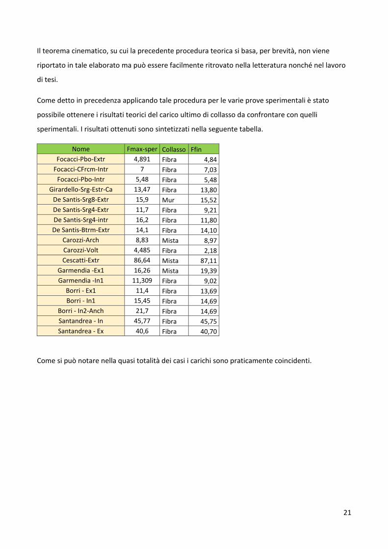
Il teorema cinematico, su cui la precedente procedura teorica si basa, per brevità, non viene
riportato in tale elaborato ma può essere facilmente ritrovato nella letteratura nonché nel lavoro
di tesi.
Come detto in precedenza applicando tale procedura per le varie prove sperimentali è stato
possibile ottenere i risultati teorici del carico ultimo di collasso da confrontare con quelli
sperimentali. I risultati ottenuti sono sintetizzati nella seguente tabella.
Nome Fmax-sper Collasso Ffin
Focacci-Pbo-Extr 4,891 Fibra 4,84
Focacci-CFrcm-Intr 7 Fibra 7,03
Focacci-Pbo-Intr 5,48 Fibra 5,48
Girardello-Srg-Estr-Ca 13,47 Fibra 13,80
De Santis-Srg8-Extr 15,9 Mur 15,52
De Santis-Srg4-Extr 11,7 Fibra 9,21
De Santis-Srg4-intr 16,2 Fibra 11,80
De Santis-Btrm-Extr 14,1 Fibra 14,10
Carozzi-Arch 8,83 Mista 8,97
Carozzi-Volt 4,485 Fibra 2,18
Cescatti-Extr 86,64 Mista 87,11
Garmendia -Ex1 16,26 Mista 19,39
Garmendia -In1 11,309 Fibra 9,02
Borri - Ex1 11,4 Fibra 13,69
Borri - In1 15,45 Fibra 14,69
Borri - In2-Anch 21,7 Fibra 14,69
Santandrea - In 45,77 Fibra 45,75
Santandrea - Ex 40,6 Fibra 40,70
Come si può notare nella quasi totalità dei casi i carichi sono praticamente coincidenti.
22
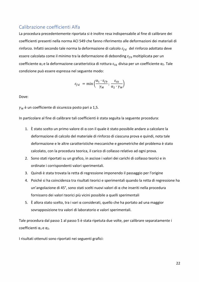
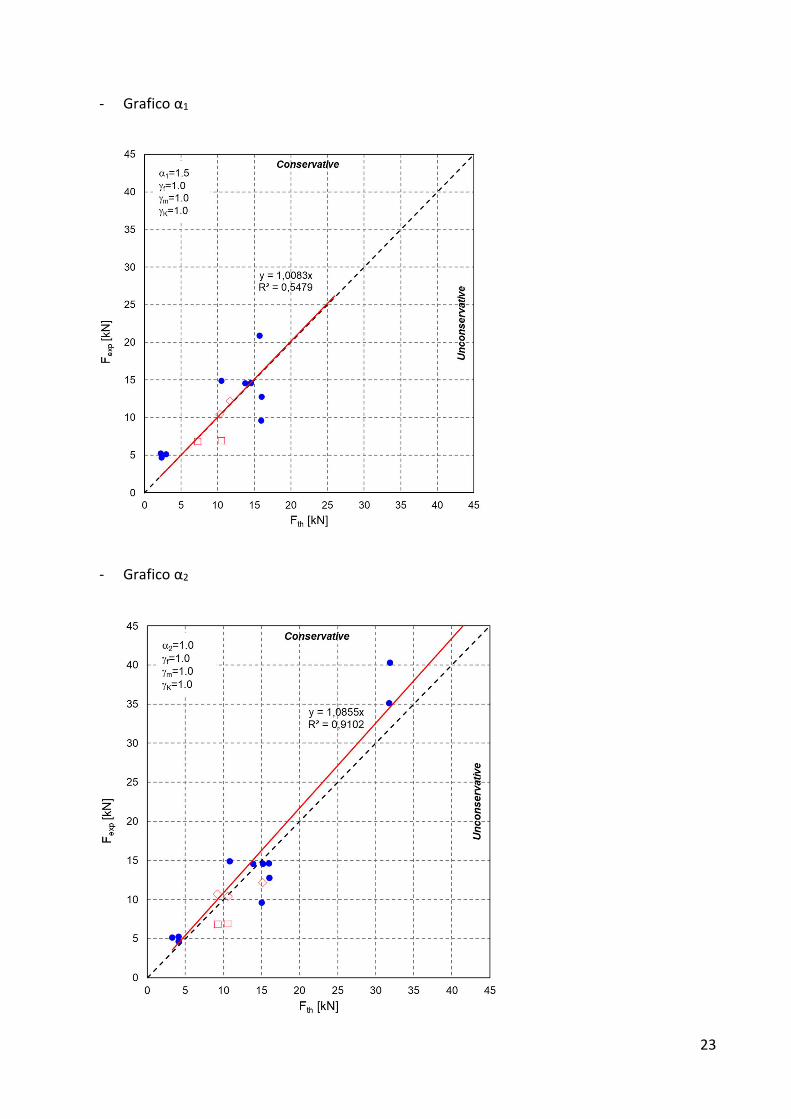
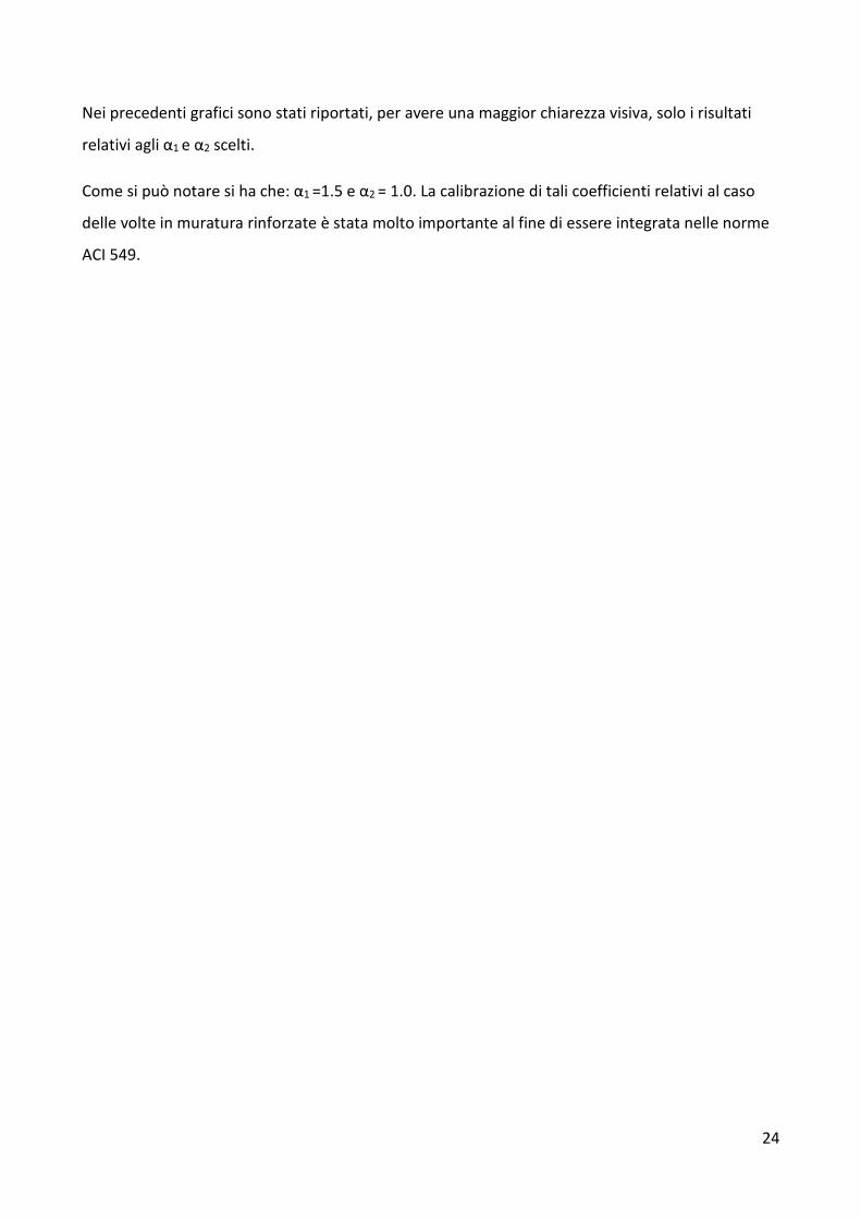
Calibrazione coefficienti Alfa
La procedura precedentemente riportata si è inoltre resa indispensabile al fine di calibrare dei
coefficienti presenti nella norma ACI 549 che fanno riferimento alle deformazioni dei materiali di
rinforzo. Infatti secondo tale norma la deformazione di calcolo ��� del rinforzo adottato deve
essere calcolata come il minimo tra la deformazione di debonding � moltiplicata per un
coefficiente α1 e la deformazione caratteristica di rottura ε�� divisa per un coefficiente α2. Tale
condizione può essere espressa nel seguente modo:
��� = min α� ∙ ε����
; ε��α� ∙ ��
�
Dove:
�� è un coefficiente di sicurezza posto pari a 1,5.
In particolare al fine di calibrare tali coefficienti è stata seguita la seguente procedura:
1. È stato scelto un primo valore di α con il quale è stato possibile andare a calcolare la
deformazione di calcolo del materiale di rinforzo di ciascuna prova e quindi, nota tale
deformazione e le altre caratteristiche meccaniche e geometriche del problema è stato
calcolato, con la procedura teorica, il carico di collasso relativo ad ogni prova.
2. Sono stati riportati su un grafico, in ascisse i valori dei carichi di collasso teorici e in
ordinate i corrispondenti valori sperimentali.
3. Quindi è stata trovata la retta di regressione imponendo il passaggio per l’origine
4. Poiché si ha coincidenza tra risultati teorici e sperimentali quando la retta di regressione ha
un’angolazione di 45°, sono stati scelti nuovi valori di α che inseriti nella procedura
fornissero dei valori teorici più vicini possibile a quelli sperimentali
5. È allora stato scelto, tra i vari α considerati, quello che ha portato ad una maggior
sovrapposizione tra valori di laboratorio e valori sperimentali.
Tale procedura dal passo 1 al passo 5 è stata ripetuta due volte, per calibrare separatamente i
coefficienti α1 e α2.
I risultati ottenuti sono riportati nei seguenti grafici:
23
- Grafico α1
- Grafico α2
24
Nei precedenti grafici sono stati riportati, per avere una maggior chiarezza visiva, solo i risultati
relativi agli α1 e α2 scelti.
Come si può notare si ha che: α1 =1.5 e α2 = 1.0. La calibrazione di tali coefficienti relativi al caso
delle volte in muratura rinforzate è stata molto importante al fine di essere integrata nelle norme
ACI 549.