Tutorial Number 20: Pulsating flow in a bifurcated vessel ... Abaqus tutorial Pulsating flow...

Simuleon B.V.

Sint Antoniestraat 7 5314 LG Bruchem

T. +31(0)418-644699 F. +31(0)418-644690 E. [email protected] W. www.simuleon.nl

Tutorial Number 20:

Pulsating flow in a bifurcated vessel with Abaqus/CFD

Ramin Riahi

June 2015

Simuleon B.V.


T. +31(0)418-644699 F. +31(0)418-644690 E. [email protected] W. www.simuleon.nl 2

1. Introduction

In this tutorial, you will create a transient fluid dynamic analysis of a bifurcated

artery with Abaqus/CFD.

When you complete this tutorial, you will be able to:

- Create transient and steady state Abaqus/CFD analyses.

- Discretize the geometry and insert a mesh boundary layer.

- Define material model for a non Newtonian fluid for blood modelling.

- Define a parabolic profile at the inlet and outlet.

- Define pulsating fluid boundary conditions.

Preliminaries

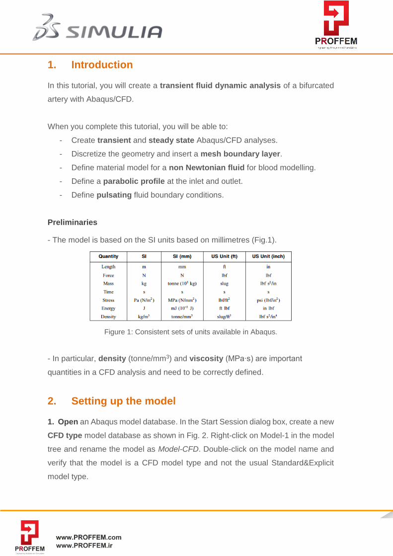
- The model is based on the SI units based on millimetres (Fig.1).

Figure 1: Consistent sets of units available in Abaqus.

- In particular, density (tonne/mm3) and viscosity (MPa∙s) are important

quantities in a CFD analysis and need to be correctly defined.

2. Setting up the model

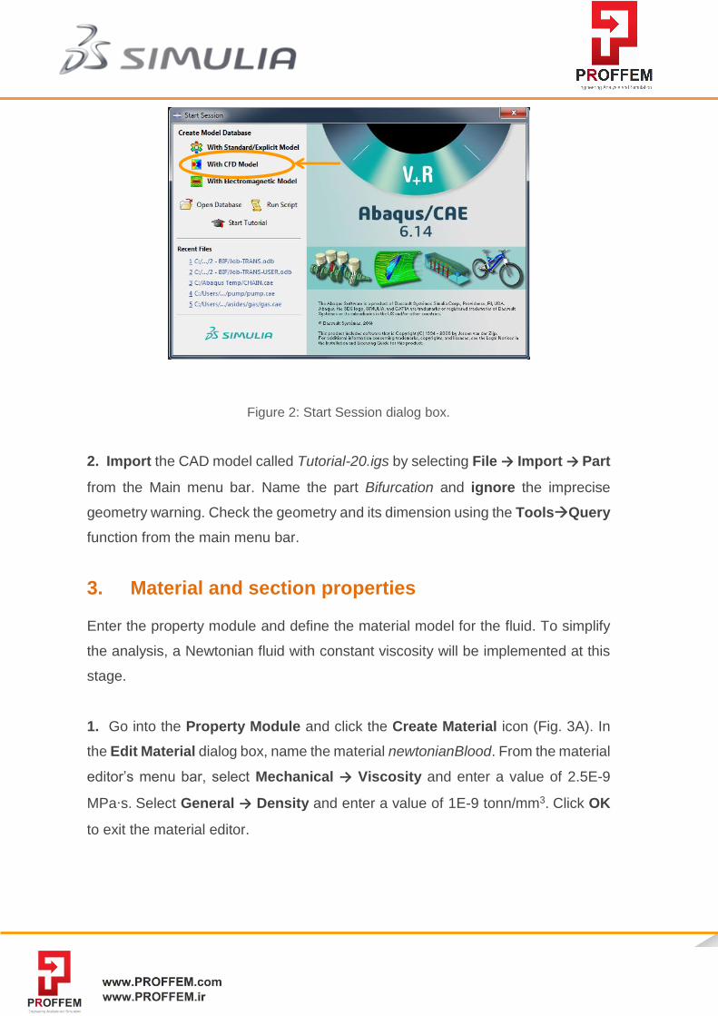
1. Open an Abaqus model database. In the Start Session dialog box, create a new

CFD type model database as shown in Fig. 2. Right-click on Model-1 in the model

tree and rename the model as Model-CFD. Double-click on the model name and

verify that the model is a CFD model type and not the usual Standard&Explicit

model type.

Simuleon B.V.



Figure 2: Start Session dialog box.

2. Import the CAD model called Tutorial-20.igs by selecting File → Import → Part

from the Main menu bar. Name the part Bifurcation and ignore the imprecise

geometry warning. Check the geometry and its dimension using the ToolsQuery

function from the main menu bar.

3. Material and section properties

Enter the property module and define the material model for the fluid. To simplify

the analysis, a Newtonian fluid with constant viscosity will be implemented at this

stage.

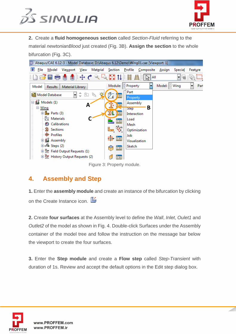
1. Go into the Property Module and click the Create Material icon (Fig. 3A). In

the Edit Material dialog box, name the material newtonianBlood. From the material

editor’s menu bar, select Mechanical → Viscosity and enter a value of 2.5E-9

MPa∙s. Select General → Density and enter a value of 1E-9 tonn/mm3. Click OK

to exit the material editor.

Simuleon B.V.



2. Create a fluid homogeneous section called Section-Fluid referring to the

material newtonianBlood just created (Fig. 3B). Assign the section to the whole

bifurcation (Fig. 3C).

Figure 3: Property module.

4. Assembly and Step

1. Enter the assembly module and create an instance of the bifurcation by clicking

on the Create Instance icon.

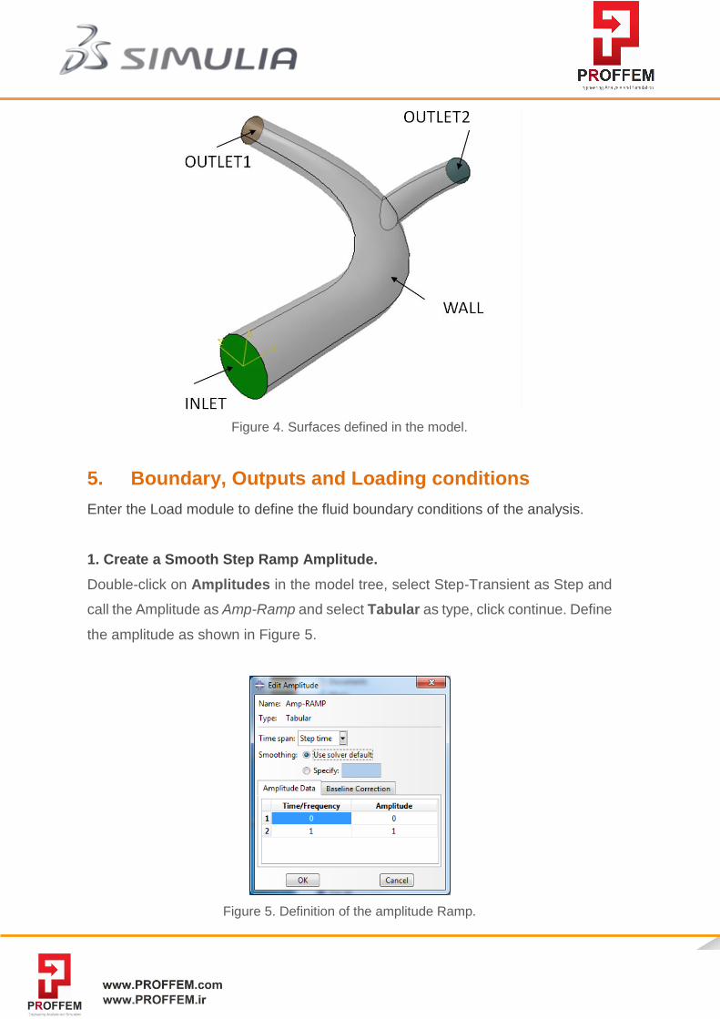
2. Create four surfaces at the Assembly level to define the Wall, Inlet, Oulet1 and

Outlet2 of the model as shown in Fig. 4. Double-click Surfaces under the Assembly

container of the model tree and follow the instruction on the message bar below

the viewport to create the four surfaces.

3. Enter the Step module and create a Flow step called Step-Transient with

duration of 1s. Review and accept the default options in the Edit step dialog box.

A B

C

Simuleon B.V.



Figure 4. Surfaces defined in the model.

5. Boundary, Outputs and Loading conditions

Enter the Load module to define the fluid boundary conditions of the analysis.

1. Create a Smooth Step Ramp Amplitude.

Double-click on Amplitudes in the model tree, select Step-Transient as Step and

call the Amplitude as Amp-Ramp and select Tabular as type, click continue. Define

the amplitude as shown in Figure 5.

Figure 5. Definition of the amplitude Ramp.

Simuleon B.V.



2. Create a Wall boundary condition.

Double-click on BCs in the model tree, call the BC as BC-WALL, select the Step-

Transient as step, Fluid as Category and Fluid wall condition as Type. In the

Prompt bar below the viewport, click on the Button Surfaces and select the

previously defined surface called WALL. Accept the default No slip condition and

click Ok.

3. Create a velocity BC at the Inlet.

Double-click on BCs in the model tree, call the BC as BC-INLET, select the Step-

Transient as step, Fluid as Category and Fluid Inlet/Outlet as Type. Select the

previously defined surface called INLET and specify a Velocity condition with V1

equal to 0.1 mm/s and V2 and V3 equal to 0. Select the Amp-Ramp as Amplitude

click Ok.

4. Create a velocity BC at the Outlet1.

Double-click on BCs in the model tree, call the BC as BC-OUTLET1, select the

Step-Transient as step, Fluid as Category and Fluid Inlet/Outlet as Type. Select

the previously defined surface called OUTLET1 and specify a Velocity condition

with V2 equal to 0.082 mm/s and V1 and V3 equal to 0. Select the Amp-Ramp as

Amplitude click Ok. This condition corresponds to a 55% of the initial flow rate.

5. Create a pressure BC at the Outlet2.

Double-click on BCs in the model tree, call the BC as BC-INLET, select the Step-

Transient as step, Fluid as Category and Fluid Inlet/Outlet as Type. Select the

previously defined surface called OUTLET2 and specify a Pressure condition

equal to 0. Click Ok.

6. Create the Initial Predefined Velocity Field.

Click on Predefined Fields in the model tree. Select Initial as the Step, Fluid as

category and Fluid velocity as type, click Continue. Select the Whole model as

region and accept 0 as velocity in all directions. Click OK.

Simuleon B.V.



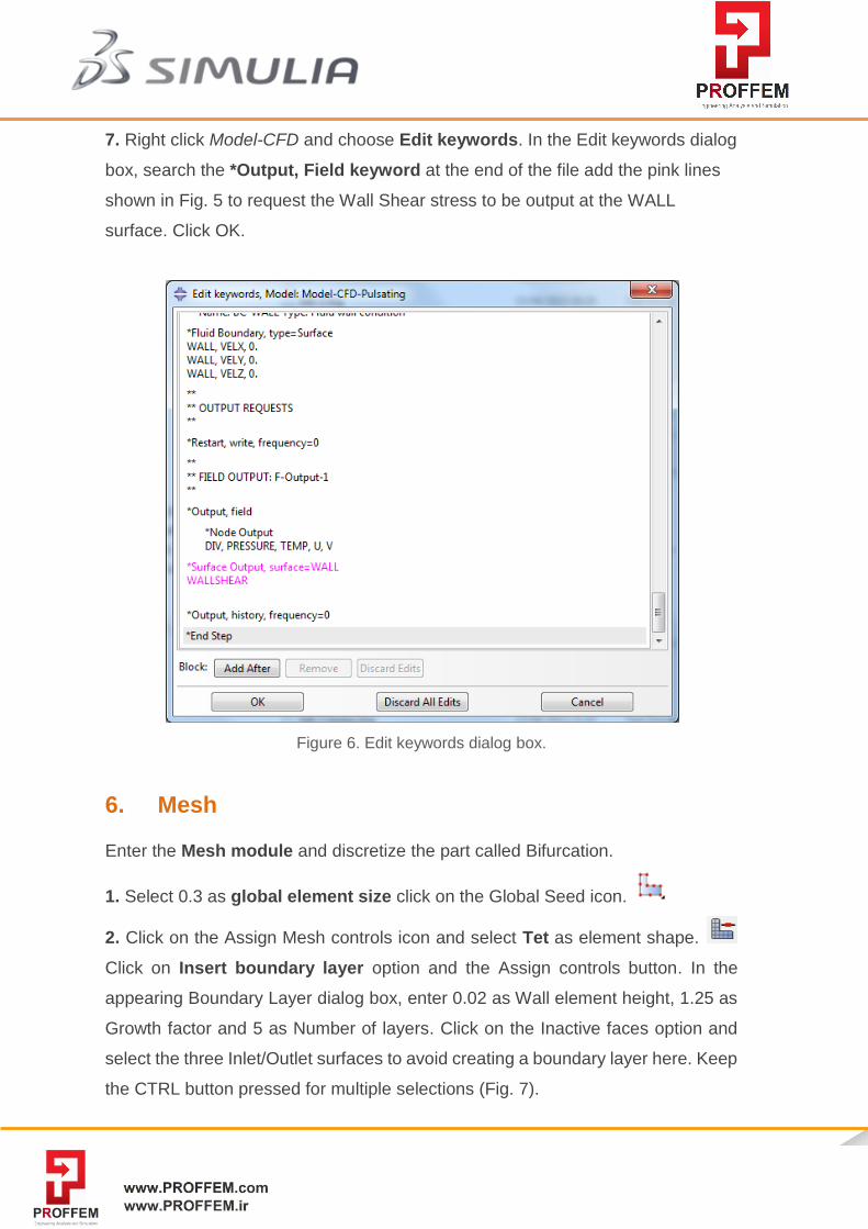
7. Right click Model-CFD and choose Edit keywords. In the Edit keywords dialog

box, search the *Output, Field keyword at the end of the file add the pink lines

shown in Fig. 5 to request the Wall Shear stress to be output at the WALL

surface. Click OK.

Figure 6. Edit keywords dialog box.

6. Mesh

Enter the Mesh module and discretize the part called Bifurcation.

1. Select 0.3 as global element size click on the Global Seed icon.

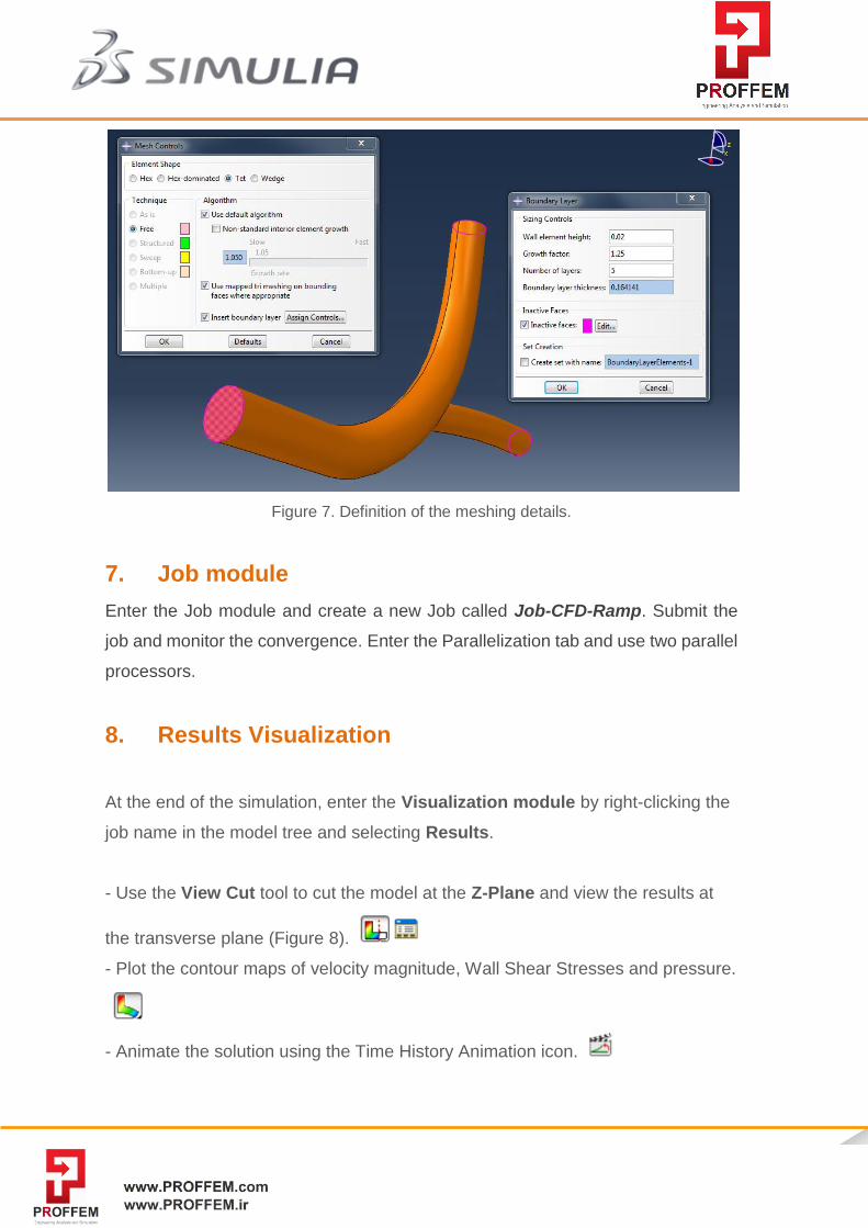
2. Click on the Assign Mesh controls icon and select Tet as element shape.

Click on Insert boundary layer option and the Assign controls button. In the

appearing Boundary Layer dialog box, enter 0.02 as Wall element height, 1.25 as

Growth factor and 5 as Number of layers. Click on the Inactive faces option and

select the three Inlet/Outlet surfaces to avoid creating a boundary layer here. Keep

the CTRL button pressed for multiple selections (Fig. 7).

Simuleon B.V.



Figure 7. Definition of the meshing details.

7. Job module

Enter the Job module and create a new Job called Job-CFD-Ramp. Submit the

job and monitor the convergence. Enter the Parallelization tab and use two parallel

processors.

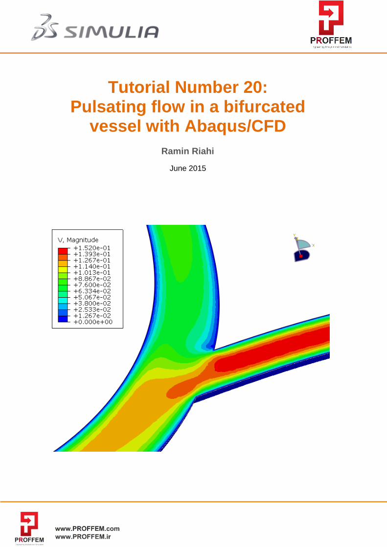
8. Results Visualization

At the end of the simulation, enter the Visualization module by right-clicking the

job name in the model tree and selecting Results.

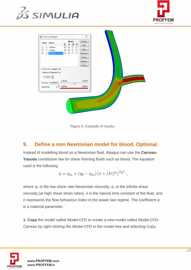
- Use the View Cut tool to cut the model at the Z-Plane and view the results at

the transverse plane (Figure 8).

- Plot the contour maps of velocity magnitude, Wall Shear Stresses and pressure.

- Animate the solution using the Time History Animation icon.

Simuleon B.V.



Figure 8. Example of results.

9. Define a non Newtonian model for blood. Optional.

Instead of modelling blood as a Newtonian fluid, Abaqus can use the Carreau-

Yasuda constitutive law for shear thinning fluids such as blood. The equation

used is the following

where η0 is the low shear rate Newtonian viscosity, η∞ is the infinite shear

viscosity (at high shear strain rates), λ is the natural time constant of the fluid, and

n represents the flow behaviour index in the power law regime. The coefficient α

is a material parameter.

1. Copy the model called Model-CFD to create a new model called Model-CFD-

Carreau by right-clicking the Model-CFD in the model tree and selecting Copy.

Simuleon B.V.



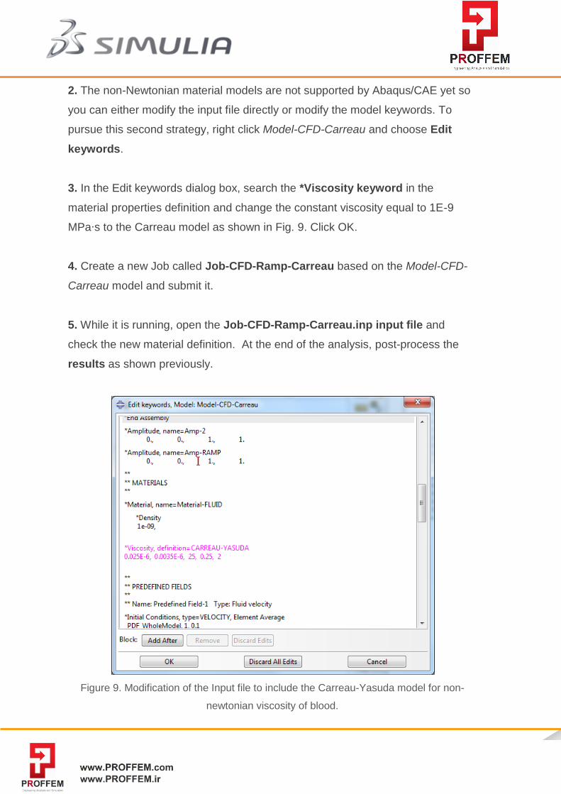
2. The non-Newtonian material models are not supported by Abaqus/CAE yet so

you can either modify the input file directly or modify the model keywords. To

pursue this second strategy, right click Model-CFD-Carreau and choose Edit

keywords.

3. In the Edit keywords dialog box, search the *Viscosity keyword in the

material properties definition and change the constant viscosity equal to 1E-9

MPa∙s to the Carreau model as shown in Fig. 9. Click OK.

4. Create a new Job called Job-CFD-Ramp-Carreau based on the Model-CFD-

Carreau model and submit it.

5. While it is running, open the Job-CFD-Ramp-Carreau.inp input file and

check the new material definition. At the end of the analysis, post-process the

results as shown previously.

Figure 9. Modification of the Input file to include the Carreau-Yasuda model for non-

newtonian viscosity of blood.

Simuleon B.V.



10. Define a paraboloid profile. Optional.

A parabolic profile can be directly defined in Abaqus/CAE to avoid adding long

entrance regions in the CFD domain. To fasten the simulation, the Newtonian

blood model is used.

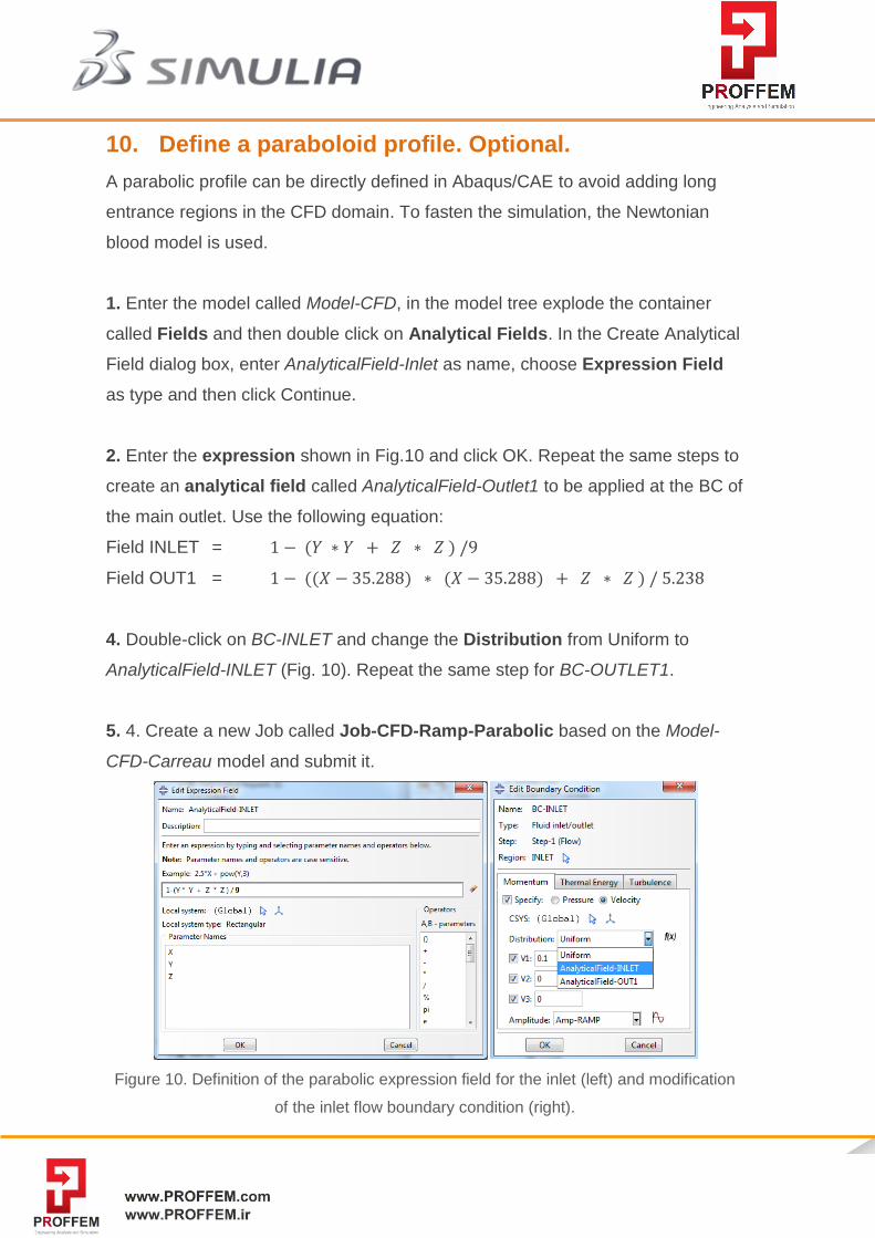
1. Enter the model called Model-CFD, in the model tree explode the container

called Fields and then double click on Analytical Fields. In the Create Analytical

Field dialog box, enter AnalyticalField-Inlet as name, choose Expression Field

as type and then click Continue.

2. Enter the expression shown in Fig.10 and click OK. Repeat the same steps to

create an analytical field called AnalyticalField-Outlet1 to be applied at the BC of

the main outlet. Use the following equation:

Field INLET = 1 − (𝑌 ∗ 𝑌 + 𝑍 ∗ 𝑍 ) /9

Field OUT1 = 1 − ((𝑋 − 35.288) ∗ (𝑋 − 35.288) + 𝑍 ∗ 𝑍 ) / 5.238

4. Double-click on BC-INLET and change the Distribution from Uniform to

AnalyticalField-INLET (Fig. 10). Repeat the same step for BC-OUTLET1.

5. 4. Create a new Job called Job-CFD-Ramp-Parabolic based on the Model-

CFD-Carreau model and submit it.

Figure 10. Definition of the parabolic expression field for the inlet (left) and modification

of the inlet flow boundary condition (right).

Simuleon B.V.



11. Define a pulsating profile. Optional.

In this section, you will create a pulsating profile using a periodic amplitude

definition. To fasten the simulation, the Newtonian blood model is used.

1. Copy the model called Model-CFD to create a new model called Model-CFD-

Pulsating by right-clicking the Model-CFD in the model tree and selecting Copy.

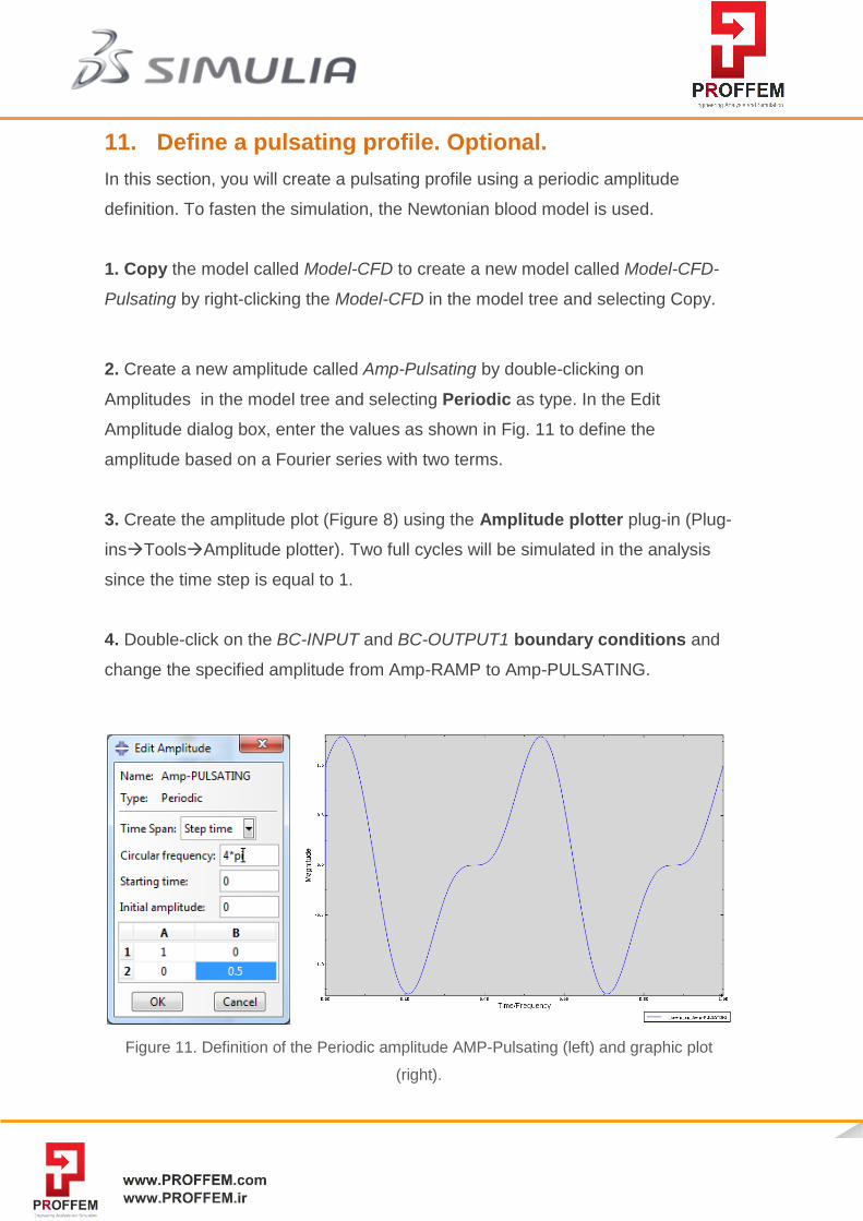
2. Create a new amplitude called Amp-Pulsating by double-clicking on

Amplitudes in the model tree and selecting Periodic as type. In the Edit

Amplitude dialog box, enter the values as shown in Fig. 11 to define the

amplitude based on a Fourier series with two terms.

3. Create the amplitude plot (Figure 8) using the Amplitude plotter plug-in (Plug-

insToolsAmplitude plotter). Two full cycles will be simulated in the analysis

since the time step is equal to 1.

4. Double-click on the BC-INPUT and BC-OUTPUT1 boundary conditions and

change the specified amplitude from Amp-RAMP to Amp-PULSATING.

Figure 11. Definition of the Periodic amplitude AMP-Pulsating (left) and graphic plot

(right).

Simuleon B.V.



4. Create a new Job called Job-CFD-Pulsating based on the Model-CFD-

Pulsating model and submit it.

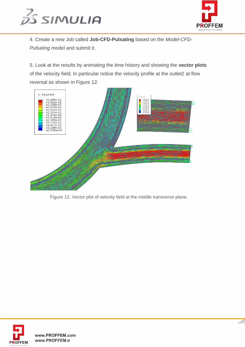
5. Look at the results by animating the time history and showing the vector plots

of the velocity field. In particular notice the velocity profile at the outlet2 at flow

reversal as shown in Figure 12.

Figure 12. Vector plot of velocity field at the middle transverse plane.

Tutorial Number 20: Pulsating flow in a bifurcated vessel ... Abaqus tutorial Pulsating flow...

Documents

Transcript of Tutorial Number 20: Pulsating flow in a bifurcated vessel ... Abaqus tutorial Pulsating flow...