J. Astrophys. Astr. (1990) 11, 445–460 The Eccentric Double-Lined Binary BD – 1° 1004 Ν. Kameswara Rao & B. N. Ashoka* Indan Institute of Astrophysics,Bangalore, 560034

C. Lloyd, C. D. Pike & D. J. Stickland Rutherford Appleton Laboratory,Chilton, UK Received 1990 April 18; accepted 1990 August 14

Abstract. A new radial velocity study has been made of the highlyeccentric, early-type binary BD –1° 1004 using spectra from the Kavalur Observatory. All available archival material has also been reexamined. An attempt has been made to correct for line ‘dragging’ by the secondary spectrum to improve the fit of the observed data to the orbital solutions. It is found that an earlier suggestion of apsidal regression is still possible although ω is probably constant within the errors. There remain problemsand inconsistencies with other orbital elements, in particular K1 and γ. Key words: stars, spectroscopic binaries—stars, radial velocities—stars,individual

1. Introduction

Direct observational studies of stellar structure fall broadly into two camps. The most heavily exploited relies upon measurements of radial and non-radial pulsation to give clues as to the nature of the underlying strata, an approach which has made significant strides in recent years with the development of sensitive instrumentation for stellar seismology led, naturally, by work on the Sun.

The other direction is that of the determination and interpretation of the advance ofthe line of apsides in binaries with eccentric orbits. Unfortunately, there are selection effects which have prevented this second approach from making a major impact although it has the merit of being applicable to stars considerably fainter than those presently required for seismological investigation (and thus permitting examination of a wider sample of spectral types). The first is that the most accurate measures accrue from eclipsing binaries and these, by dint of their generally relatively small separation, tend to be in circular orbits. On the other hand, apsidal motions derived fromspectroscopic orbits generally require a prodigious amount of observing sustained,even if in somewhat staccato fashion, over many years. The latter can also be confounded by uncertainty over the values of ω, especially where the eccentricity is small, as for example in the case of AO Cas (Stickland & Lloyd 1988).

In the case of spectroscopic binaries with large eccentricity, provided that sufficient data exist over an appropriately long baseline—a condition realized with the

*Present address: ISRO Satellite Centre, Bangalore 560017.

446 Ν. Κ. Rao et al. availability of IUE archival data (cf. Harvey et al. 1987), some progress ought to be forthcoming. This appeared to be the case for the massive binary ι Orionis (Stickland et al. 1987) where a value of 0.41 ± 0.07 deg / 1000 days was derived, leading to an apsidal constant, K2, of 0.0023. However, a cautionary note was sounded in that paper concerning the apparently strange apsidal behaviour of a rather similar system, BD – 1° 1004 (= HR 1952, B2 IV, mv =4.95),in which the published values of ω seemed to decrease with time.

The motivation for this present study was to reexamine the orbital elements for thissystem, adding in a new set from data secured in the last few years. Along the way, it became apparent that the determination of some of the elements was being confused by the presence of the secondary spectrum and perhaps other effects, and that such manifestations might have wider implications, particularly with regard to the Barr Effect in which there appears a non-random distribution of longitudes of periastron in the catalogues of binary orbital elements.

2. Previous determinations of orbital elements

The binary nature of BD –1° 1004 was established by Frost (1906) who secured four spectrograms at Yerkes Observatory in 1905/6, which showed a range of over 160 km s–1 and implied a short period, although with hindsight we note that theobservations which lead to this conclusion straddle the sharp change at periastron. He saw no evidence of a secondary although the He I line at 4388 Å gave an anomalous displacement.

Following up their work on ι Ori, Plaskett & Harper (1909) described a study ofboth systems in an important work which was to foreshadow many problems in the future associated with systems in which the secondary is luminous enough to interfere with measurements of the primary spectrum. They presented orbital elements of BD – 1° 1004 based on 36 spectrograms gathered between the end of 1907 and early 1909 but incorporating Frost's data in order to achieve a better estimate of the period. Unfortunately neither the original measures nor the spectrograms appear to be extant and we have to be content with the 14 normal places given in their paper. As they stood, these data failed to provide a satisfactory solution and recourse was made to using a preliminary solution, fitting a sine wave with the binary period to the residuals, subtracting this from the observations and finding the final set of elements by iteration through four least-squares solutions. While this was effective in reducing the residuals to more accustomed values, the rationale for this method is not obvious and hence the meaning of the derived elements remains unclear. Suffice it to say at this juncture that they obtained a value for ω of 87°, having found 90° in the preliminary solution.

The next study came from Pearce (1953) and depended on 17 spectrograms secured near the nodes during 1941 and which afforded the luxury of measurement of the secondary. Since such spectra presumably did not suffer markedly from the ‘dragging’ which afflicts data taken nearer to the systemic velocity, no mention is made of recourse to the artifice used by Plaskett & Harper; a value of ω of 84.6° ± 3° was obtained. The mass ratio, m1 /m2, deduced by Pearce was 0.64 with an estimatedmagnitude difference in the blue of 1.14. Again it is to be regretted that Pearce did not present his measurements for reexamination, and not even the normal points appear in the brief abstract, but fortunately we have been able to borrow, through the kind

Double-lined binary BD – 1° 1004 447

offices of Dr. Alan Batten, the original spectrograms; our remeasurement of these is described below.

The final set of published elements for BD — 1o 1004 was derived from 86 platestaken at Haute Provence in the early 1950s and analysed by Mme. Barbier-Brossat (1954), hot on the heels of the work of Pearce and apparently independent of it. Once more only normal points were published but through the generosity of the Director of l’Observatoire de Haute Provence, the spectrograms were available for remeasure- ment. Mme. Barbier used two least squares iterations, deriving an ω of 76°.

From these determinations, it may be that while a consistent solution can beproduced either by careful selection of the data to be used or by post facto and somewhat ad hoc manipulation, use of the raw measurements in a conventional solution might imply apsidal regression. If the latter is correct, then it needs to be confirmed by observations at a much later epoch; if ω is really constant, then some quantitative explanation needs to be forthcoming for the form of the corrections applied.

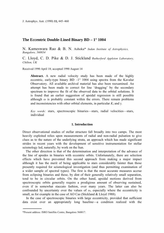
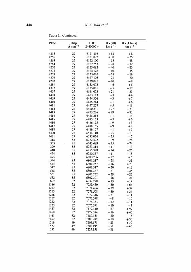
3. New observations An extensive series of new observations has been made at Kavalur Observatory in the period from the end of 1984 to the beginning of 1988. The majority of these plates was taken at a dispersion of 27 Å mm–1 and a journal of the observations is given in Table1. They were scanned with the PDS machine at the Indian Institute of Astrophysics at Bangalore and the tape sent to the Rutherford Appleton Laboratory where measure- ments were made using the program PICA on the STARLINK computer. In general,even at the higher dispersions and at times of maximum or minimum velocity, signatures of the secondary component were not obvious and consistent asymmetriesin all the lines were not readily apparent. For this reason, the lines were measured as

Table 1. Radial-velocity observations of BD – 1o 1004 from

Kavalur.

448 N. K. Rao et al.

Table 1. Continued.

Double-lined binary BD – 1° 1004 449

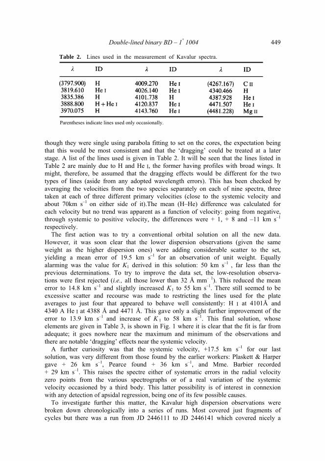
Table 2. Lines used in the measurement of Kavalur spectra.

Parentheses indicate lines used only occasionally.

though they were single using parabola fitting to set on the cores, the expectation being that this would be most consistent and that the ‘dragging’ could be treated at a later stage. A list of the lines used is given in Table 2. It will be seen that the lines listed in Table 2 are mainly due to Η and He I, the former having profiles with broad wings. Itmight, therefore, be assumed that the dragging effects would be different for the two types of lines (aside from any adopted wavelength errors). This has been checked by averaging the velocities from the two species separately on each of nine spectra, three taken at each of three different primary velocities (close to the systemic velocity and about 70km s–1 on either side of it).The mean (H–He) difference was calculated for each velocity but no trend was apparent as a function of velocity: going from negative, through systemic to positive velocity, the differences were + 1, + 8 and –11 km s–1

respectively. The first action was to try a conventional orbital solution on all the new data.

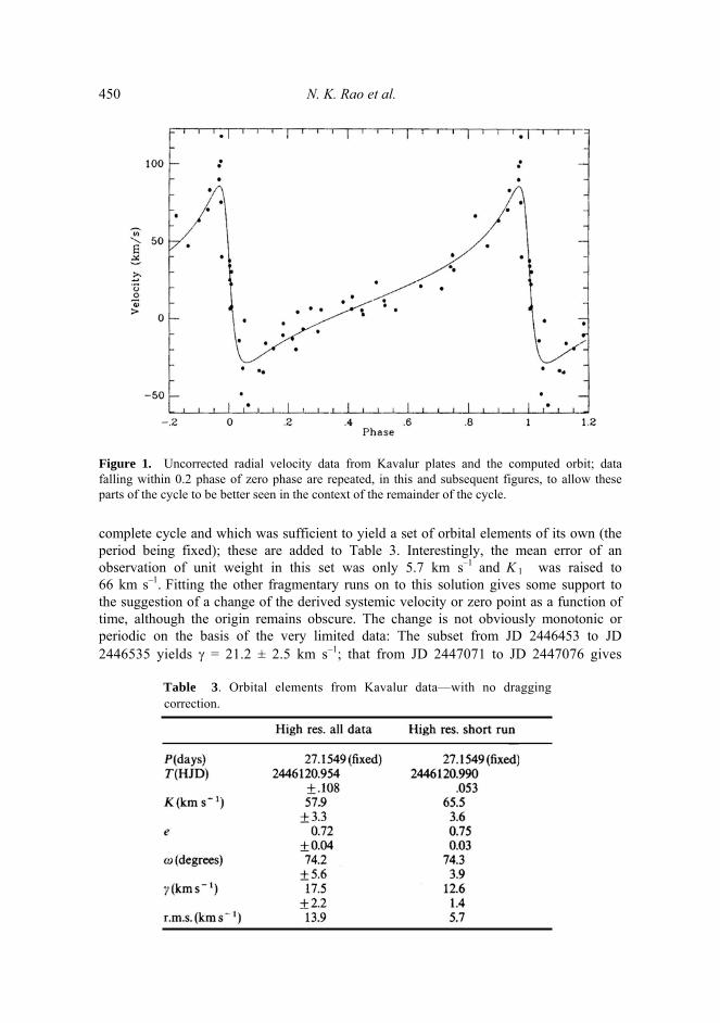
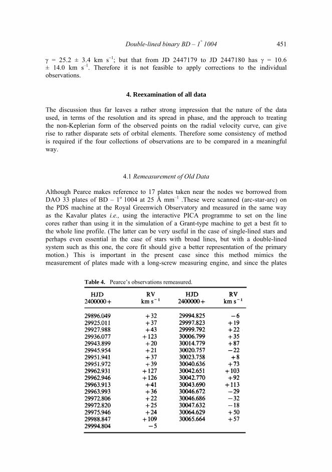
However, it was soon clear that the lower dispersion observations (given the same weight as the higher dispersion ones) were adding considerable scatter to the set, yielding a mean error of 19.5 km s–1 for an observation of unit weight. Equally alarming was the value for K1 derived in this solution: 50 km s–1 , far less than the previous determinations. To try to improve the data set, the low-resolution observa- tions were first rejected (i.e., all those lower than 32 Å mm– 1). This reduced the mean error to 14.8 km s–1 and slightly increased K1 to 55 km s–1. There still seemed to beexcessive scatter and recourse was made to restricting the lines used for the plate averages to just four that appeared to behave well consistently: Η I at 4101Å and4340 A He I at 4388 Å and 4471 Å. This gave only a slight further improvement of theerror to 13.9 km s–1 and increase of K 1 to 58 km s–1. This final solution, whose elements are given in Table 3, is shown in Fig. 1 where it is clear that the fit is far from adequate; it goes nowhere near the maximum and minimum of the observations andthere are notable ‘dragging’ effects near the systemic velocity.

A further curiosity was that the systemic velocity, +17.5 km s–1 for our last solution, was very different from those found by the earlier workers: Plaskett & Harper gave + 26 km s–1, Pearce found + 36 km s–1, and Mme. Barbier recorded + 29 km s–1. This raises the spectre either of systematic errors in the radial velocity zero points from the various spectrographs or of a real variation of the systemic velocity occasioned by a third body. This latter possibility is of interest in connexion with any detection of apsidal regression, being one of its few possible causes.

To investigate further this matter, the Kavalur high dispersion observations werebroken down chronologically into a series of runs. Most covered just fragments ofcycles but there was a run from JD 2446111 to JD 2446141 which covered nicely a

450 N. K. Rao et al.

Figure 1. Uncorrected radial velocity data from Kavalur plates and the computed orbit; datafalling within 0.2 phase of zero phase are repeated, in this and subsequent figures, to allow these parts of the cycle to be better seen in the context of the remainder of the cycle.

complete cycle and which was sufficient to yield a set of orbital elements of its own (the period being fixed); these are added to Table 3. Interestingly, the mean error of an observation of unit weight in this set was only 5.7 km s–1 and K 1 was raised to66 km s–1. Fitting the other fragmentary runs on to this solution gives some support to the suggestion of a change of the derived systemic velocity or zero point as a function of time, although the origin remains obscure. The change is not obviously monotonic or periodic on the basis of the very limited data: The subset from JD 2446453 to JD 2446535 yields γ = 21.2 ± 2.5 km s–1; that from JD 2447071 to JD 2447076 gives

Table 3. Orbital elements from Kavalur data—with no draggingcorrection.

Double-lined binary BD – 1° 1004 451

γ = 25.2 ± 3.4 km s–1; but that from JD 2447179 to JD 2447180 has γ = 10.6± 14.0 km s–1. Therefore it is not feasible to apply corrections to the individual observations.

4. Reexamination of all data

The discussion thus far leaves a rather strong impression that the nature of the data used, in terms of the resolution and its spread in phase, and the approach to treating the non-Keplerian form of the observed points on the radial velocity curve, can giverise to rather disparate sets of orbital elements. Therefore some consistency of method is required if the four collections of observations are to be compared in a meaningful way.

4.1 Remeasurement of Old Data

Although Pearce makes reference to 17 plates taken near the nodes we borrowed from DAO 33 plates of BD – 1o

1004 at 25 Å mm–1 .These were scanned (arc-star-arc) onthe PDS machine at the Royal Greenwich Observatory and measured in the same way as the Kavalur plates i.e., using the interactive PICA programme to set on the line cores rather than using it in the simulation of a Grant-type machine to get a best fit to the whole line profile. (The latter can be very useful in the case of single-lined stars and perhaps even essential in the case of stars with broad lines, but with a double-lined system such as this one, the core fit should give a better representation of the primary motion.) This is important in the present case since this method mimics the measurement of plates made with a long-screw measuring engine, and since the plates

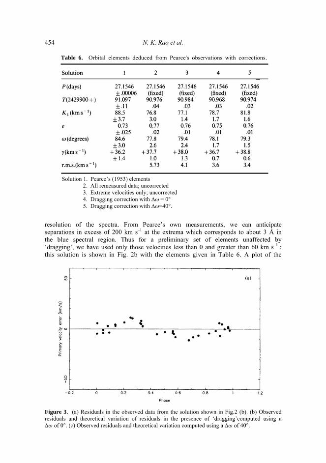
Table 4. Pearce’s observations remeasured.

452 Ν. Κ. Rao et al.

Table 5. Barbier’s observations remeasured.

of Plaskett & Harper are not available for study, one needs an approach that would be compatible with their probable technique. Ten photospheric lines of Η I and He I weremeasured and the results are presented with a journal of Pearce’s observations inTable 4.

We were also able to remeasure the 38 Å mm– 1 plates from Haute Provence used byMme. Barbier. These too were scanned on the PDS at RGO and were measured in a similar fashion although the process was made more efficient by setting up a template to direct the search for line cores so that the fitting could be done automatically. 77 spectrograms were thus examined although ten of these could not be used (due to underexposure, weak arc lines etc.); these are reported in Table 5.

4.2 Reanalysis off Pearce’s Observations

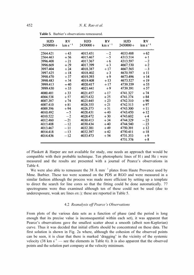
From plots of the various data sets as a function of phase (and the period is long enough that its precise value is inconsequential within each set), it was apparent that Pearce’s observations gave the smallest scatter about a smooth (albeit non-Keplerian) curve. Thus it was decided that initial efforts should be concentrated on these data. The first solution is shown in Fig. 2a where, although the cohesion of the observed points can be seen, it is clear that there is marked ‘dragging’ in the vicinity of the systemic velocity (38 km s–1 — see the elements in Table 6). It is also apparent that the observed points and the solution part company at the velocity minimum.

Double-lined binary BD – 1° 1004 453

Figrue 2. (a) The orbit using all the radial velocities from the remeasuredobservation of Pearce (b) The orbit computed using only the extreme velocities (although alldata points are shown). Since in Pearce’s observations the secondary spectrum can be seen at velocity extrema, one must assume that it is having an effect on measurements of the primaryspectrum, to a greater or lesser degree, all the time. However, if one measures the linecores, then there is the prospect that for velocities separated suffciently from the systemic velocity, an accurate estimate of the primary velocity can be obtained. This naturally depends on the line widths, which will be influenced by rotation, and on the

454 Ν. Κ. Rao et al.

Table 6. Orbital elements deduced from Pearce's observations with corrections.

Solution 1. Pearce’s (1953) elements 2. All remeasured data; uncorrected 3. Extreme velocities only; uncorrected 4. Dragging correction with ∆ω = 0° 5. Dragging correction with ∆ω=40°.

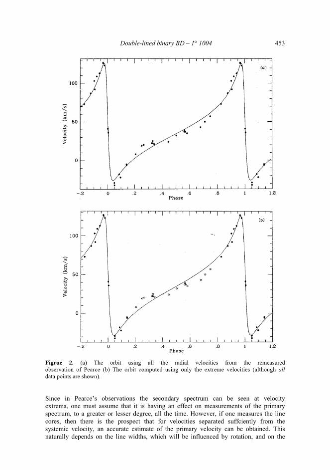
resolution of the spectra. From Pearce’s own measurements, we can anticipate separations in excess of 200 km s–1 at the extrema which corresponds to about 3 Å in the blue spectral region. Thus for a preliminary set of elements unaffected by ‘dragging’, we have used only those velocities less than 0 and greater than 60 km s–1 ; this solution is shown in Fig. 2b with the elements given in Table 6. A plot of the

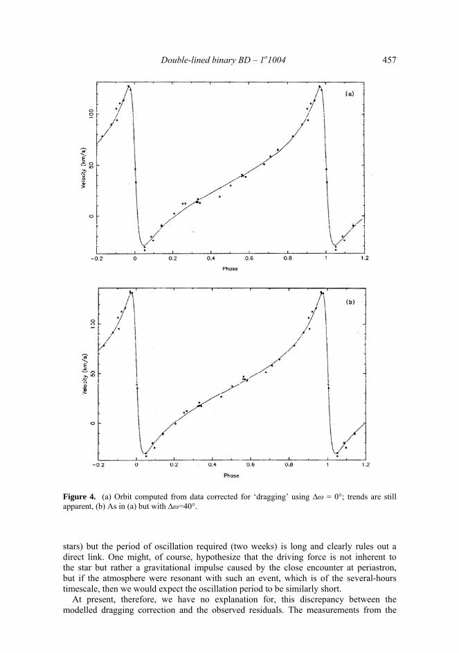
Figure 3. (a) Residuals in the observed data from the solution shown in Fig.2 (b). (b) Observedresiduals and theoretical variation of residuals in the presence of ‘dragging’computed using a ∆ω of 0°. (c) Observed residuals and theoretical variation computed using a ∆ω of 40°.

Double-lined binary BD – 1o 1004 455

Figure 3. Continued.

residual velocities from such a fit is shown in Fig. 3a. As might be expected,the detailedsolution from such a data set is sensitive to exactly which data are included. In order to eliminate this problem it is necessary to correct the blended velocities before solving for the orbital parameters. If this can be done then all observed velocities can be included in the solution.

An attempt to model the deviations from Keplerian motion has been made in the following way—an approach similar to that described by Tatum (1968) and Griffin (1986). A typical spectral line was assumed to have a Lorentz profile with a width of

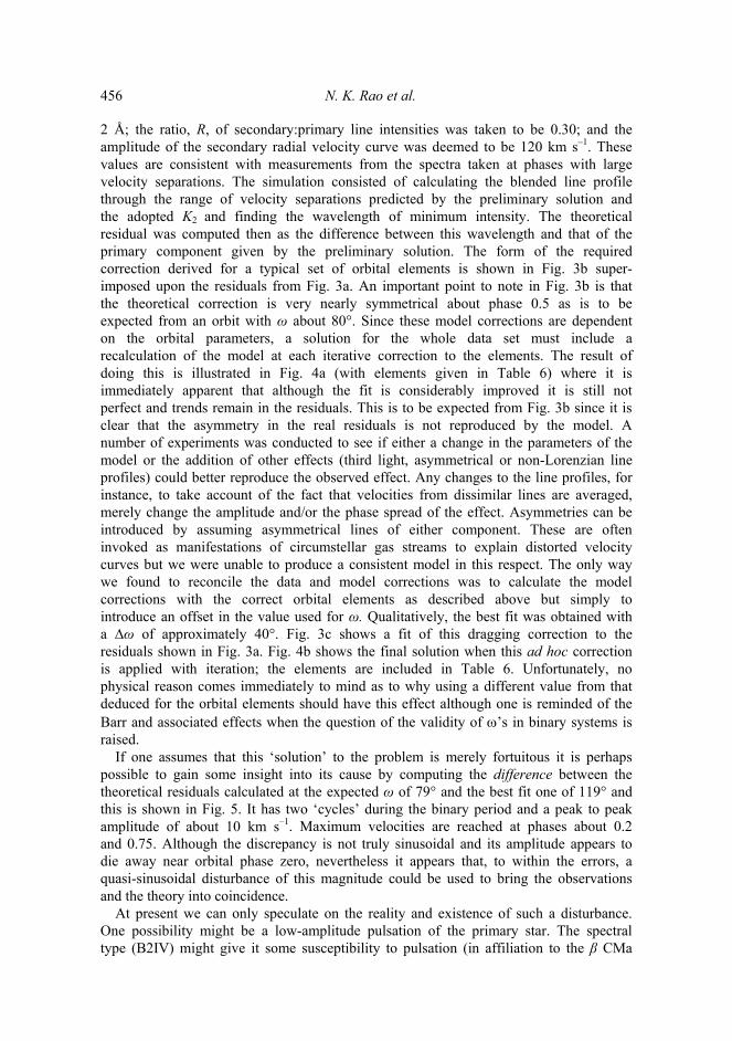
456 Ν. Κ. Rao et al. 2 Å; the ratio, R, of secondary:primary line intensities was taken to be 0.30; and the amplitude of the secondary radial velocity curve was deemed to be 120 km s–1. Thesevalues are consistent with measurements from the spectra taken at phases with large velocity separations. The simulation consisted of calculating the blended line profile through the range of velocity separations predicted by the preliminary solution and the adopted K2 and finding the wavelength of minimum intensity. The theoretical residual was computed then as the difference between this wavelength and that of the primary component given by the preliminary solution. The form of the required correction derived for a typical set of orbital elements is shown in Fig. 3b super- imposed upon the residuals from Fig. 3a. An important point to note in Fig. 3b is that the theoretical correction is very nearly symmetrical about phase 0.5 as is to be expected from an orbit with ω about 80°. Since these model corrections are dependent on the orbital parameters, a solution for the whole data set must include a recalculation of the model at each iterative correction to the elements. The result of doing this is illustrated in Fig. 4a (with elements given in Table 6) where it is immediately apparent that although the fit is considerably improved it is still not perfect and trends remain in the residuals. This is to be expected from Fig. 3b since it is clear that the asymmetry in the real residuals is not reproduced by the model. A number of experiments was conducted to see if either a change in the parameters of the model or the addition of other effects (third light, asymmetrical or non-Lorenzian line profiles) could better reproduce the observed effect. Any changes to the line profiles, for instance, to take account of the fact that velocities from dissimilar lines are averaged, merely change the amplitude and/or the phase spread of the effect. Asymmetries can be introduced by assuming asymmetrical lines of either component. These are often invoked as manifestations of circumstellar gas streams to explain distorted velocity curves but we were unable to produce a consistent model in this respect. The only way we found to reconcile the data and model corrections was to calculate the model corrections with the correct orbital elements as described above but simply to introduce an offset in the value used for ω. Qualitatively, the best fit was obtained with a ∆ω of approximately 40°. Fig. 3c shows a fit of this dragging correction to the residuals shown in Fig. 3a. Fig. 4b shows the final solution when this ad hoc correction is applied with iteration; the elements are included in Table 6. Unfortunately, no physical reason comes immediately to mind as to why using a different value from that deduced for the orbital elements should have this effect although one is reminded of the Barr and associated effects when the question of the validity of ω’s in binary systems israised.

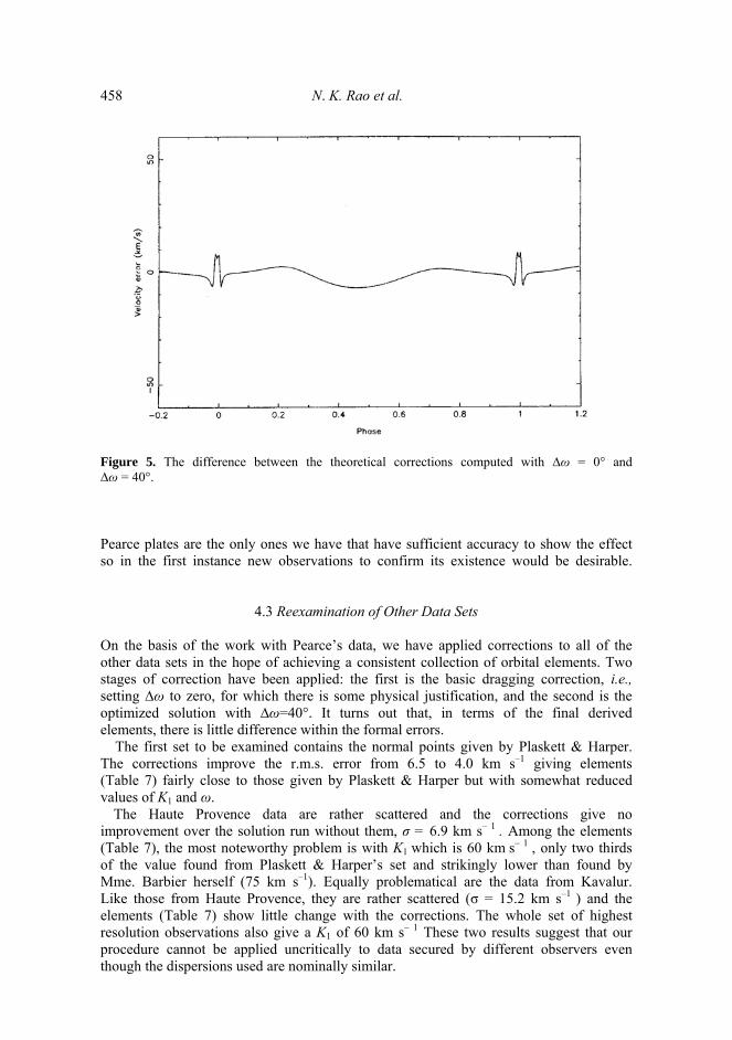
If one assumes that this ‘solution’ to the problem is merely fortuitous it is perhaps possible to gain some insight into its cause by computing the difference between the theoretical residuals calculated at the expected ω of 79° and the best fit one of 119° and this is shown in Fig. 5. It has two ‘cycles’ during the binary period and a peak to peak amplitude of about 10 km s–1. Maximum velocities are reached at phases about 0.2 and 0.75. Although the discrepancy is not truly sinusoidal and its amplitude appears to die away near orbital phase zero, nevertheless it appears that, to within the errors, a quasi-sinusoidal disturbance of this magnitude could be used to bring the observations and the theory into coincidence.

At present we can only speculate on the reality and existence of such a disturbance.One possibility might be a low-amplitude pulsation of the primary star. The spectral type (B2IV) might give it some susceptibility to pulsation (in affiliation to the β CMa

Double-lined binary BD – 1o1004 457

Figure 4. (a) Orbit computed from data corrected for ‘dragging’ using ∆ω = 0°; trends are still apparent, (b) As in (a) but with ∆ω=40°.

stars) but the period of oscillation required (two weeks) is long and clearly rules out a direct link. One might, of course, hypothesize that the driving force is not inherent to the star but rather a gravitational impulse caused by the close encounter at periastron, but if the atmosphere were resonant with such an event, which is of the several-hours timescale, then we would expect the oscillation period to be similarly short.

At present, therefore, we have no explanation for, this discrepancy between the modelled dragging correction and the observed residuals. The measurements from the

458 N. Κ. Rao et al.

Figure 5. The difference between the theoretical corrections computed with ∆ω = 0° and ∆ω = 40°.

Pearce plates are the only ones we have that have sufficient accuracy to show the effect so in the first instance new observations to confirm its existence would be desirable.

4.3 Reexamination of Other Data Sets

On the basis of the work with Pearce’s data, we have applied corrections to all of the other data sets in the hope of achieving a consistent collection of orbital elements. Two stages of correction have been applied: the first is the basic dragging correction, i.e.,setting ∆ω to zero, for which there is some physical justification, and the second is the optimized solution with ∆ω=40°. It turns out that, in terms of the final derived elements, there is little difference within the formal errors.

The first set to be examined contains the normal points given by Plaskett & Harper. The corrections improve the r.m.s. error from 6.5 to 4.0 km s–1 giving elements (Table 7) fairly close to those given by Plaskett & Harper but with somewhat reduced values of K1 and ω.

The Haute Provence data are rather scattered and the corrections give no improvement over the solution run without them, σ = 6.9 km s– 1 . Among the elements (Table 7), the most noteworthy problem is with K1 which is 60 km s– 1 , only two thirds of the value found from Plaskett & Harper’s set and strikingly lower than found by Mme. Barbier herself (75 km s–1). Equally problematical are the data from Kavalur. Like those from Haute Provence, they are rather scattered (σ = 15.2 km s–1 ) and the elements (Table 7) show little change with the corrections. The whole set of highest resolution observations also give a K1 of 60 km s– 1 These two results suggest that our procedure cannot be applied uncritically to data secured by different observers even though the dispersions used are nominally similar.

Double-lined binary BD –1o 1004 459 Table 7. Orbital elements deduced from all data with corrections (∆ω = 0).

Solution 1, Plaskett & Harper’s data 2. Pearce’s data (Solution 4 of Table 5) 3. Haute Provence data 4. Kavalur data 5. All data normalized to γ = + 37 km s–1 (Pearce’s value).

5. Conclusions

We have described in some detail attempts to model the effects of line dragging in the spectrum of BD –1° 1004 because there is a number of such systems whose orbital elements are astrophysically valuable but for which rather ad hoc corrections have been applied in the past. While we feel that some progress in matching the observations has been made, the fitting is not yet satisfactory and further investigation may be desirable. However, the main recommendation is for such systems to be observed at higher resolution and signal-to-noise ratio.

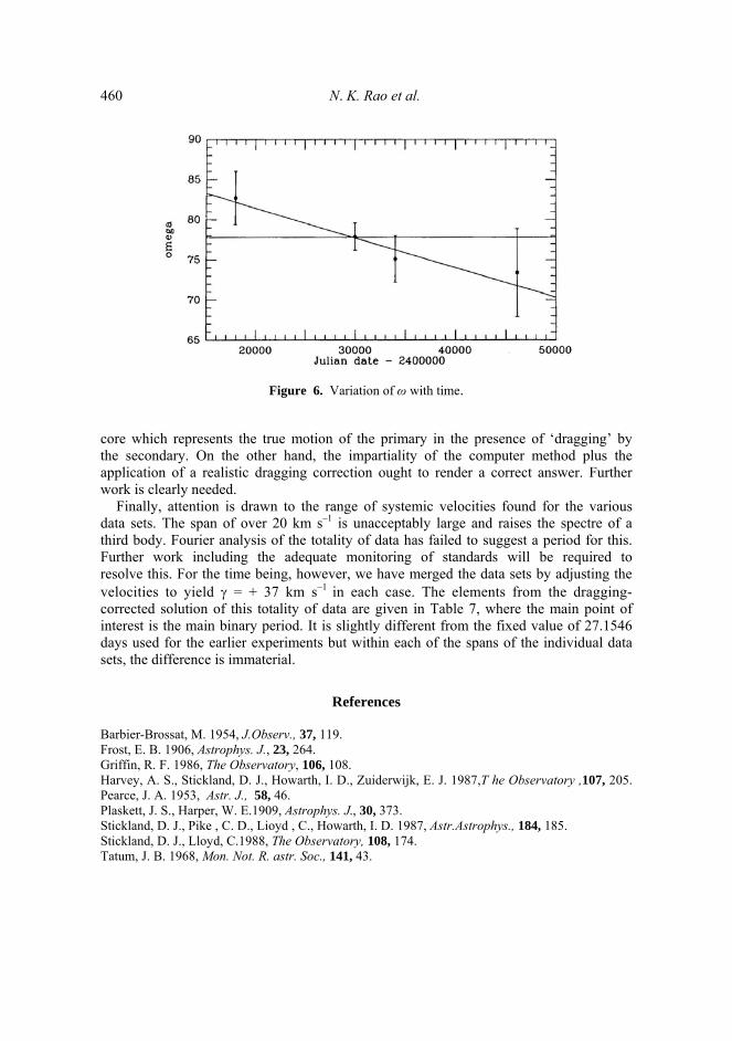
The results presented in Table 7 suggest that the value of ω is constant, within the errors, at about 78°, although one might formally claim a slow regression—see Fig. 6 with ω = – 0.38° ± 0.08° per 1000 days. The determination of any apsidal motion was a major aim of this work and so it is disappointing to leave the question somewhat open. One comment that can be made, however, concerns the value of comparing ω’sfrom different data sets where different values of e are also produced, the latter being, of course, unacceptable astrophysically. Using a program originating from Dr G. Hill at DAO and made available through Drs Bell and Hilditch at St. Andrews, it has been possible to take a representative set of data and, over a plausible range of parameters, determine the independence (or otherwise) of e and ω. In the present instance, for a run of e from 0.65 through to 0.80, the change in ω was less than 1.5°, smaller than the typical formal error. Thus the finding above regarding apsidal motion cannot be masked by errors in e in the individual solutions.

The matter of the disparate values of Κ1 is of some considerable concern and the difference between the original measurements, presumably carried out by eye, and the modern results using a density scan of the spectrum suggests a fundamental difference in what is being measured. It may imply that the eye is better able to pick out the line

460 N. Κ. Rao et al.

Figure 6. Variation of ω with time.

core which represents the true motion of the primary in the presence of ‘dragging’ by the secondary. On the other hand, the impartiality of the computer method plus the application of a realistic dragging correction ought to render a correct answer. Further work is clearly needed.

Finally, attention is drawn to the range of systemic velocities found for the variousdata sets. The span of over 20 km s–1 is unacceptably large and raises the spectre of a third body. Fourier analysis of the totality of data has failed to suggest a period for this. Further work including the adequate monitoring of standards will be required to resolve this. For the time being, however, we have merged the data sets by adjusting the velocities to yield γ = + 37 km s–1

in each case. The elements from the dragging-corrected solution of this totality of data are given in Table 7, where the main point of interest is the main binary period. It is slightly different from the fixed value of 27.1546 days used for the earlier experiments but within each of the spans of the individual datasets, the difference is immaterial.

References

Barbier-Brossat, M. 1954, J.Observ., 37, 119. Frost, E. B. 1906, Astrophys. J., 23, 264. Griffin, R. F. 1986, The Observatory, 106, 108. Harvey, A. S., Stickland, D. J., Howarth, I. D., Zuiderwijk, E. J. 1987,T he Observatory ,107, 205.Pearce, J. A. 1953, Astr. J., 58, 46. Plaskett, J. S., Harper, W. E.1909, Astrophys. J., 30, 373. Stickland, D. J., Pike , C. D., Lioyd , C., Howarth, I. D. 1987, Astr.Astrophys., 184, 185. Stickland, D. J., Lloyd, C.1988, The Observatory, 108, 174. Tatum, J. Β. 1968, Mon. Not. R. astr. Soc., 141, 43.