1

THE DOPING PHASE DIAGRAM OF Y 1-xCaxBa2(Cu1-yZny)3O7-δ

FROM TRANSPORT MEASUREMENTS: TRACKING

THE PSEUDOGAP BELOW Tc (y = 0)

S.H. Naqib1*, J.R. Cooper1 and J.L. Tallon2

1IRC in Superconductivity, University of Cambridge, Madingley Road, Cambridge CB3 OHE, UK2MacDiarmid Institute for Advanced Materials and Nanotechnology, Victoria University and Industrial Research Ltd.,

P.O. Box 31310, Lower Hutt, New Zealand

*Corresponding author: Phone: +44–1223-337049; Fax: +44-1223-337074; E-mail: shn21@hermes.cam.ac.uk

Abstract

The effects of planar hole concentration, p, on the resistivity, ρ(T), of sintered Y1-

xCaxBa2(Cu1-yZny)3O7-δ samples were investigated over a wide range of Ca, Zn, and

oxygen contents. Zn was used to suppress superconductivity and this enabled us to

extract the characteristic pseudogap temperature, T*(p), from ρ(T,p) data below Tco(p) [ ≡

Tc (y = 0)]. We have also located the characteristic temperature, Tscf, marking the onset of

significant superconducting fluctuations above Tc, from the analysis of ρ(T,H,p) and

ρ(T,p) data. This enabled us to identify T*(p) near the optimum doping level where the

values of T*(p) and Tscf(p) are very close and hard to distinguish. We again found that

T*(p) depends only on the hole concentration p, and not on the level of disorder

associated with Zn or Ca substitutions. We conclude that (i) T*(p) (and therefore, the

pseudogap) persists below Tco(p) on the overdoped side and does not merge with the

Tco(p) line and (ii) T*(p), and thus the pseudogap energy, extrapolates to zero at the

doping p = 0.19 ± 0.01.

PACS numbers: 74.25.Dw, 74.25. 74.62.Dh, 74.72.-h

2

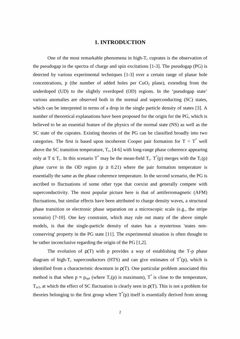
1. INTRODUCTION

One of the most remarkable phenomena in high-Tc cuprates is the observation of

the pseudogap in the spectra of charge and spin excitations [1-3]. The pseudogap (PG) is

detected by various experimental techniques [1-3] over a certain range of planar hole

concentrations, p (the number of added holes per CuO2 plane), extending from the

underdoped (UD) to the slightly overdoped (OD) regions. In the ‘pseudogap state’

various anomalies are observed both in the normal and superconducting (SC) states,

which can be interpreted in terms of a drop in the single particle density of states [3]. A

number of theoretical explanations have been proposed for the origin for the PG, which is

believed to be an essential feature of the physics of the normal state (NS) as well as the

SC state of the cuprates. Existing theories of the PG can be classified broadly into two

categories. The first is based upon incoherent Cooper pair formation for T < T* well

above the SC transition temperature, Tc, [4-6] with long-range phase coherence appearing

only at T ≤ Tc. In this scenario T* may be the mean-field Tc. T*(p) merges with the Tc(p)

phase curve in the OD region (p ≥ 0.21) where the pair formation temperature is

essentially the same as the phase coherence temperature. In the second scenario, the PG is

ascribed to fluctuations of some other type that coexist and generally compete with

superconductivity. The most popular picture here is that of antiferromagnetic (AFM)

fluctuations, but similar effects have been attributed to charge density waves, a structural

phase transition or electronic phase separation on a microscopic scale (e.g., the stripe

scenario) [7-10]. One key constraint, which may rule out many of the above simple

models, is that the single-particle density of states has a mysterious 'states non-

conserving' property in the PG state [11]. The experimental situation is often thought to

be rather inconclusive regarding the origin of the PG [1,2].

The evolution of ρ(T) with p provides a way of establishing the T-p phase

diagram of high-Tc superconductors (HTS) and can give estimates of T*(p), which is

identified from a characteristic downturn in ρ(T). One particular problem associated this

method is that when p ≈ popt (where Tc(p) is maximum), T* is close to the temperature,

Tscf, at which the effect of SC fluctuation is clearly seen in ρ(T). This is not a problem for

theories belonging to the first group where T*(p) itself is essentially derived from strong

3

SC fluctuations. For the second scenario, this poses a problem as SC fluctuations (and

superconductivity itself) mask the signatures of the predicted PG in the vicinity of (and

below) Tc. With the notable exception of specific heat measurements [3], most

experimental techniques are unable to track the predicted T*(p) below Tc(p). One way of

avoiding this problem is to suppress superconductivity with a magnetic field and reveal

the ’NS’ below Tc, because the PG is comparatively insensitive to magnetic field [12]. In

practice this is very difficult because of the very large upper critical field, Hc2, of many

HTS. The other way is to destroy superconductivity by introducing disorder, e.g., by

alloying with Zn. Because of the d-wave order parameter, Zn substitution suppresses

superconductivity most effectively and, like a magnetic field, has little effect on T*(p)

[13]. We took this second route to look for T*(p) below Tco(p).

In this paper we report a systematic study of the transport properties of the

superconducting compound Y1-xCaxBa2(Cu1-yZny)3O7-δ. We have measured resistivity,

room-temperature thermopower, S[290K], and the AC susceptibility (ACS) of a series of

sintered Y1-xCaxBa2(Cu1-yZny)3O7-δ samples with different levels of Zn, Ca, and oxygen

contents. The motivation for the present study is to locate T*(p) from the evolution of

ρ(T) of Y123 with different amounts of Zn and Ca extending from UD to OD states.

While pure Y123 with full oxygenation (δ = 0), is slightly OD, further overdoping can be

achieved by substituting Y3+ by Ca2+. The advantages of using Zn are: (i) it mainly

substitutes the in-plane Cu(2) sites, thus the effects of planar impurity can be studied and

(ii) the doping level remains nearly the same when Cu(2) is substituted by Zn, enabling

one to look at the effects of disorder on various normal and SC state properties at almost

the same hole concentration [14,15]. From the analysis of ρ(T,p) and ρ(T,p,H) data we

extracted the p-dependence of the characteristic temperatures T*and Tscf, and find that

indeed T* falls below Tco providing strong evidence for the second scenario, namely that

the PG arises from an independent coexisting correlation.

2. EXPERIMENTAL DETAILS AND RESULTS

Single-phase polycrystalline sintered samples of Y1-xCaxBa2(Cu1-yZny)3O7-δ were

synthesized in both laboratories by solid-state reaction methods using high-purity (>

4

99.99%) powders. The details of sample preparation and characterization can be found in

refs. [16,17]. The NS and SC properties, including T*, of HTS are highly sensitive to p

and, therefore, it is important to determine p as accurately as possible. The room

temperature thermopower, S[290K], has a systematic variation with p for various HTS

over the entire doping range extending from very UD to heavily OD regimes [18], also

S[290K] is insensitive to in-plane disorder like Zn and the crystalline state of the sample

[19]. For these reasons S[290K] is a good measure of p even in the presence of strong in-

plane scattering by Zn2+ ions. For all our samples we have used S[290K]⊗ [20] to

determine p. Using these values of p, we find that the parabolic Tc(p) formula [21], given

by

is obeyed for all samples. Usually, for Zn-free samples, Z and popt seem to take on

universal values but these parameters increase systematically with increasing Zn content

[22]. In the present case, Z increases from the usual 82.6 [21] for the Zn-free sample to

410 for 6%-Zn sample [22] and popt rises from 0.16 for the Zn-free compound [21] to

0.174 for the 6%Zn-20%Ca sample [22]. The physical meaning of these changes in the

fitting parameters is that as the Zn content is increased, the region of superconductivity

shrinks and becomes centred on higher values of p, before finally forming a small bubble

around p ~ 0.19 and disappearing completely for y ~ 0.1 [23]. From the observed

evolution of popt(y) we previously inferred that superconductivity for this system is at its

strongest at p ~ 0.185 (Fig.1 of ref.[22]), as this remains the last point of

superconductivity at a critical Zn concentration (defined as the highest possible Zn

concentration for which superconductivity just survives, considering all p-values). This

point has been made earlier in other studies [22,23] and the value p ~ 0.19 is indeed a

special value at which the PG vanishes quite abruptly, as seen from the analysis of

specific heat data of HTS cuprates [11,23].

⊗ S[290K] = -139p + 24.2 for p > 0.155

S[290K] = 992exp(-38.1p) for 0.155 ≥ p > 0.05

(1) 2)(1)(

)(opt

optc

c ppZpT

pT −−=

5

The hole concentration was varied by changing both the oxygen deficiency and

the Ca content. We have obtained Tc from both resistivity and low field (Hrms = 0.1Oe; f

= 333.3Hz) ACS measurements. Tc was taken at zero resistance (within the noise level of

± 10-6 Ω) and at the point where the line drawn on the steepest part of diamagnetic ACS

curve meets the T-independent base line associated with the negligibly small NS signal.

Tc-values obtained from these two methods agree within 1K for most of the samples [22].

We placed particular emphasis on the determination of p and Tc as accurately as possible

because of the extreme sensitivity of various ground-state SC and NS properties to p.

This is especially true near the optimum doping level, where, although Tc(p) is nearly

flat, the SC condensation energy, superfluid density, PG energy scale etc. change quite

abruptly and substantially for a small change in p [11,23-25].

Sintered bars of 89 to 93% of the theoretical density were used for resistivity

measurements. Resistivity was measured using the four-terminal method with an ac

current of 1 mA (77 Hz) using 40 µm dia. copper wire and silver paint to make the

contacts. Typical contact resistances were below 2Ω. Transformers were used to

minimize electrical noise. We have tried to locate the PG temperature, T*, with a high

degree of accuracy. At this point we should emphasise that T*(p) does not represent a

phase transition temperature but instead kBT*(p) is some kind of a characteristic energy

scale of a lightly-doped Mott-insulator, probably reflecting the energy of correlated holes

and spins [11]. Plots of dρ(T)/dT vs. T and ρ(T) - ρLF vs. T yield very similar T* values

(within ± 5K) (ρLF is a linear fit ρLF = b+cT, in the high-T linear region of ρ(T), above

T*) [22]. Using T*/T as a scaling parameter, it is possible to normalize ρ(T). The result of

the scaling was shown in ref. [22], where, leaving aside the SC transitions, all resistivity

curves collapsed reasonably well on to one p-independent universal curve over a wide

temperature range. It is important to note that Zn does not change the T*(p) values but it

suppresses Tc(p) very effectively. For example, T*(p ~ 0.115) ~ 250 ± 5K for both Zn-

free and the 3%-Zn samples but Tc itself is suppressed from 70K (Zn-free) to 29K (3%-

Zn) [22]. Similar results have been obtained for Zn-substituted Y123 by other studies

[13]. This very different p-dependence for Tc and T* has often been stated as an

indication for the non-SC origin of the PG [26].

6

Magneto-transport measurements were made using an Oxford Instruments

superconducting magnet system. The sample temperature was measured using a Cernox

thermometer with an absolute accuracy of ~ 50mK. We have located Tscf, from the

analysis of ρ(T,H) and d2ρ(T)/dT2 vs. T data, in the T-range from Tc to ~ Tc + 30K. Here

we have used the facts that (i) ρ(T,H) becomes strongly field sensitive below Tscf, where

experimentally we find that conventional SC fluctuations set in quite abruptly, but T* is

unaffected by magnetic field, at least for H < 10 Tesla [12] and (ii) ρ(T) shows a much

stronger, and progressively accelerating, downturn at Tscf than that present at T*. Plots of

d2ρ(T)/dT2 vs. T mask the PG feature and visually enhance the effects of SC fluctuations

near Tscf. This is clearly seen in Fig.1, where ρ(T) of a Zn-free UD sample (p ~ 0.124 and

T* ~ 230K) has been well fitted to the form a+bT+cT2 in the temperature range of 300K >

T > Tscf. Figs.2 show the results of analysis of ρ(T) data for the extraction of Tscf for some

of the samples. Three different methods (including subtraction of a linear fit of ρ(T) to

locate the onset of the strong deviation in ρ(T) from linearity near the superconducting

transition) are applied and all of them give the same value of Tscf to within ± 2.5K.

Fig.3 shows Tc(p) and Tscf(p) of two representative 20%-Ca samples with 0%-Zn

and 4%-Zn. ∆Tscf(p) is relatively insensitive of Zn content (y) (see the inset of Fig.3), this

quantity was also found to be independent of Ca content (x) and crystalline state of the

samples (analysis of published ρ(T) data of single crystal c-axis films of Y1-

xCaxBa2Cu3O7-δ [27] and YBa2(Cu1-yZny)3O7-δ [28] gave values of ∆Tscf(p) to within ±

2K, of those found for our sintered polycrystalline samples). We have tried to model the

evolution of ∆Tscf(p) roughly from the temperature dependence of ρ at high temperatures

and from the form of the Aslamazov - Larkin (AL) contribution to the fluctuation

conductivity [29]. We show this in Fig.4. The excess conductivity due to superconducting

fluctuation, ∆σ(T), can be defined as, ∆σ(T) = 1/ρ(T) - 1/ρBG(T), where, ρBG(T) is the

background resistivity taken as the high-T fit (T > Tc + 50K) of the ρ(T) data. The AL

contribution to the fluctuation conductivity for a two-dimensional superconductor, ∆σAL,

is expressed as, ∆σAL = [e2/(16hd)]ε-1 [29], where ε = ln(T/Tc) and d is the periodicity of

superconducting layers (d ~ 11.7c for Y123, assuming that the CuO2 bilayers fluctuate as

one unit). In this analysis we have taken Tc at zero resistivity (within the noise level).

7

Fig.4 shows the T-dependence of d2ρ(T)/dT2 and d2ρtot(T)/dT2, with 1/ρtot(T) = 1/ρBG(T)

+ ∆σAL(T). In the absence of a proper energy or a momentum cut-off [30,31], extrinsic

effects due to the grain boundary resistance in polycrystalline samples (which is included

in ρBG), and problems associated with proper identification of the mean field SC

transition temperature for samples with finite transition width, a good quantitative

agreement between ρtot(T) and ρ(T) cannot be expected [30], but nevertheless d2ρ(T)/dT2

and d2ρtot(T)/dT2 show remarkable agreement (see Fig.4). We have made some model

calculations suggesting that as long as the grain boundary resistance remains temperature

independent, it does not effect the second derivative significantly. In an effort to

understand the systematic trends in ∆Tscf shown in the inset to Fig. 3 we have examined

various terms in the second temperature derivative of ρtot(T) as follows, writing

where C = e2/(16hd), we obtain (ignoring the insignificant terms)

now, assuming -η be the threshold value of the second derivative for which we can

identify a characteristic temperature T = Tscf then the above equation becomes, after some

rearrangements

where, εscf = ln(Tscf/Tc) and ρscf = ρtot(Tscf). We have plotted the left-hand side of equation

(3) versus experimental values of ρ2(Tscf) in Fig.5 using the approximation ρtot(Tscf) ~

ρ(Tscf). A remarkably linear trend is found and this gives further credence to our

fluctuation analysis. The decreasing trend in ∆Tscf with increasing doping shown in Fig. 3

(2) C 11 1

)()(−+= ε

ρρ TBGtotT

1- 2

- ) T1

()( C d

tot

εερρ

22

2

2

≈dT

tot

(3) C

Tηρ

εε 2

23

2scf

scfscf

scf ≈+

8

is therefore primarily associated with the decreasing absolute resistivity as summarised

by eq. (3).

Once we have located Tscf, we are in a position to look at T*(p) (below Tco(p)) for

Zn substituted samples. There is one disadvantage of Zn substitution that can hamper the

identification of T* from ρ(T) measurements, namely, Zn tends to localize low-energy

quasiparticles (QP) and induces an upturn in ρ(T). This upturn starts at increasingly

higher temperatures as p decreases and, to a lesser extent, as the Zn content increases, and

thus can mask the downturn due to the PG at T* [13,22]. Indeed, the upturn temperature,

Tmin, has been found to scale with T* and is evidently associated with the pseudogap,

trending to zero as p → 0.19 [32]. In this study we have taken care of this fact by

confining our attention to the ρ(T,p) data for lower Zn contents in the underdoped region

(p < 0.14). Fig.6a shows the ρ(T) data of Y0.80Ca0.20Ba2(Cu0.96Zn0.04)3O7-δ for p = 0.175 ±

0.003. The insets of Fig.6 clearly show the downturn associated with the PG at around

80K. It should be noted that Tc of this compound is 43K and Tscf = 62.5K (see Fig.3).

Fig.6b shows a similar analysis for Y0.80Ca0.20Ba2(Cu0.985Zn0.015)3O7-δ with p = 0.178 ±

0.003. The ρ(T) features of this compound once again show a T* ~ 80K with now a Tc of

54K and Tscf = 73K. Considering the facts that T*(p) values are the same irrespective of

Ca and Zn contents (at least for the level of substitutions used in present study), and Tco-

max for pure Y123 is 93K, these T*(p) are substantially below the respective Tco(p) values

(~ 90.5K) (see Fig.7). This study, to our knowledge, is the first instance where T*(p) has

been tracked down below Tco(p) from any transport measurement, although of course this

has effectively been done earlier by analysis of specific heat data by Loram et al. [3,11]

and NMR data by Tallon et al. [33]. In Fig.7 we construct a doping ‘phase diagram‘ for

Y1-xCaxBa2(Cu1-yZny)3O7-δ, including T*(p) and the PG energy scale from some other

sources [23,34]. We have taken Eg(p)/kB from specific heat measurements [23]. Eg is the

energy scale for the PG and Eg(p)/kB ~ θT*(p), where (θ = 1.4 ± 0.1) is a certain

proportionality constant [26]. The extrapolated T*(p) goes to zero at p = 0.19 ± 0.01,

following the same trend as Eg(p)/kB.

9

3. DISCUSSION

From a careful analysis of the resistivity data we have been able to track T*(p)

below Tco(p). At this point we would like to stress that T*(p) values obtained from ρ(T)

are independent of the crystalline state and are the same for polycrystalline and single

crystal samples [22]. Considering the disorder (Zn and Ca) independence of T*(p), our

findings confirm that the PG exists in the SC region below Tc of the Zn-free samples and

T*(p) does not merge with Tc(p) in the OD region as proposed by various precursor

pairing scenarios for PG. As explained in the present work, if one is unable to distinguish

between T*(p) and Tscf(p), one can easily be lead to the wrong conclusion that T*(p)

exists for p > 0.19 and merges with Tc(p) on further overdoping. As Tscf is ~ Tc + 22K

near optimum doping level, the close proximity between Tscf and T* makes an accurate

identification of T* very difficult unless both Tc and thus Tscf are suppressed by some

means that does not affect T*. Zn serves this purpose very well. Unfortunately, we have

been unable to track T*(p) to below ~ 80K for samples with p > 0.180 with enough

accuracy. This is because T*(p) decreases very sharply with increasing p (compared with

the decrease in Tc(p) and Tscf(p), see Figs.3 and 7) and becomes very close to or even

goes below Tscf and eventually Tc(p) [3,11]. For example,

Y0.90Ca0.10Ba2(Cu0.985Zn0.015)3O7-δ with p = 0.180 ± 0.0035 has a Tc = 64K and ρ(T) is

linear over 310K to 80K, marked and accelerating downturn in ρ(T) starts at ~ 79K.

Considering that, for this hole concentration, we have ∆Tscf = 17 ± 2.5 K for all our

samples, independent of Zn concentration, then this downturn at 79K is necessarily that

associated with SC fluctuations and T* must lie below this temperature. Another example

is Y0.80Ca0.20Ba2(Cu0.96Zn0.04)3O7-δ with p = 0.184 ± 0.0035, which has Tc = 42.25K and

ρ(T) is linear over 310K to 60K. A marked and accelerating downturn in ρ(T) starts at ~

58.5K (= Tscf). Thus for this compound T* < 58.5K. Although Zn substitutions greater

than 4% can help us track T*(p) below 80K precisely, this will also increase the QP

localization at lower temperatures and may mask the PG-feature in ρ(T).

Tscf(p) has been taken as the onset temperature of detectable SC fluctuations in the

present study. The disorder independence of ∆Tscf(p) (inset of Fig.3) and a simple AL-

10

type analysis of ρ(T) data (see Fig.4) strongly support this assumption. Disorder

suppresses both Tc(p) and Tscf(p) in exactly the same way, unlike T*(p) which remains

unaffected.

4. CONCLUSIONS

In summary, we have analysed our ρ(T) data to determine the T*(p) of Y1-

xCaxBa2(Cu1-yZny)3O7-δ over a wide doping range and compositions. We have shown that

T*(p) falls below Tco(p) in the OD side, does not merge with Tc(p), and the extrapolated

T*(p) becomes zero at p = 0.19 ± 0.01. We have also extracted a characteristic

temperature, Tscf, at which SC fluctuations become detectable. It is perhaps surprising

that Tscf is so well-defined experimentally in all our samples, but the very different p and

y (Zn) dependence of T* and Tscf points towards their different origins, e.g., Tscf is related

to precursor SC, whereas T* has a non-SC origin. Our findings support the picture

proposed by Loram et al. based on their specific heat study that the PG vanishes at a

critical doping, pcrit ~ 0.19, and coexists with SC for p < 0.19 [11,23]. Recently Krasnov

et al. have reached to similar conclusions based on their intrinsic tunneling spectroscopy

studies of Bi-2212 single crystals [12,35].

ACKNOWLEDGEMENTS : We gratefully acknowledge J.W. Loram for helpful

comments and suggestions. One of us (SHN) acknowledges the financial support from

the Commonwealth Scholarship Commission (UK), Darwin College, Cambridge

Philosophical Society, Lundgren Fund, and the Department of Physics, Cambridge

University.

11

REFERENCES:

[1] B. Batlogg and C. Varma, Physics World 13, 33 (2000) and M.V. Sadovskii,

USPEKHI FIZICHESKIKH NAUK 171, 539 (2001).

[2] T. Timusk and B. Statt, Rep.Progr.Phys.62, 61 (1999).

[3] J.W. Loram, K.A. Mirza, J.R. Cooper, W.Y. Liang, and J.M. Wade J. Supercon.7,

243 (1994).

[4] V.B. Geshkenbein, L.B. Ioffe, and A.I. Larkin, Phys.Rev.B 55, 3173 (1997).

[5] V. Emery, S.A. Kivelson, and O. Zachar, Phys.Rev.B 56, 6120 (1997).

[6] J. Maly, B. Janko, and K. Levin, Phys.Rev.B 59, 1354 (1999).

[7] A.P. Kampf and J.R. Schrieffer, Phys.Rev.B 42, 7967 (1990).

[8] M. Langer, J. Schmalian, S. Grabowski, and K.H. Bennemann, Phys.Rev.Lett. 75,

4508 (1995).

[9] J.J. Deisz, D.W. Hess, and J.W. Serene, Phys.Rev.Lett. 76, 1312 (1996).

[10] J. Schmalian, D. Pines, and B. Stojkovic, Phys.Rev.Lett. 80, 3839 (1998) and

A.V. Cubukov, D. Pines, and J. Schmalian, cond-mat/0201140.

[11] J.W. Loram, K.A. Mirza, J.R. Cooper, and J.L. Tallon, J.Phys.Chem.Solids 59,

2091 (1998).

[12] V.M. Krasnov, A.E. Kovalev, A. Yurgens, and D. Winkler, Phys.Rev.Lett. 86,

2657 (2001).

[13] D.J.C. Walker, A.P. Mackenzie, and J.R. Cooper, Phys.Rev.B. 51, 15653 (1995).

[14] K. Mizuhashi, K. Takenaka, Y. Fukuzumi, and S. Uchida, Phys.Rev.B 52, 3884

(1995).

[15] H. Alloul, P. Mendels, H. Casalta, J.F. Marucco, and J. Arabski, Phys.Rev.Lett.

67, 3140 (1991).

[16] G V M Willams and J L Tallon, Phys.Rev.B 57, 8696 (1998).

[17] S.H.Naqib, Ph.D. thesis, University of Cambridge, UK, 2003.

[18] S.D. Obertelli, J.R. Cooper, and J.L. Tallon, Phys.Rev.B 46, 14928 (1992).

[19] J.L. Tallon, J.R. Cooper, P.S.I.P.N. DeSilva, G.V.M. Williams, and J.L.

Loram,Phys.Rev.Lett. 75, 4114 (1995).

12

[20] J.L. Tallon, C. Bernhard, H. Shaked, R.L. Hitterman, and J.D. Jorgensen,

Phys.Rev.B 51, 12911 (1995).

[21] M.R. Presland, J.L. Tallon, R.G. Buckley, R.S. Liu, and N.E. Flower, Physica C

176, 95 (1991).

[22] S.H.Naqib, J.R. Cooper, J.L. Tallon, and C. Panagopoulas, to be published in

Physica C (2003) and cond-mat/0209457.

[23] J.L. Tallon, J.W. Loram, G.V.M. Williams, J.R. Cooper, I.R. Fisher, J.D. Johnson,

M.P. Staines, and C. Bernhard, Phys.stat.sol. (b) 215, 531 (1999).

[24] C. Panagopoulos, B.D. Rainford, J.R. Cooper, W. Lo, J.L. Tallon, J.W. Loram, J.

Betouras, Y.S. Wang, and C.W. Chu, Phys.Rev.B. 60, 14617 (1999).

[25] C. Bernhard, J.L. Tallon, Th. Blasius, A. Golnik, and Ch. Niedermayer,

Phys.Rev.Lett. 86, 1614 (2001).

[26] J.L. Tallon and J.W. Loram, Physica C 349, 53 (2001).

[27] I.R. Fisher, Ph.D. thesis, University of Cambridge, UK, 1996.

[28] D.J.C. Walker, Ph.D. thesis, University of Cambridge, UK, 1994.

[29] L.G. Aslamazov and A.I. Larkin, Phys.Lett. 26A, 238 (1968).

[30] J.Vina, J.A. Campia, C. Carballeria, S.R. Curras, A. Maignan, M.V. Ramallo, I.

Raisnes, J.A. Veira, P. Wagner, and F. Vidal, Phys.Rev.B 65, 212509 (2002).

[31] P.P. Freitas, C.C. Tsuei, T.S. Plaskett, Phys.Rev.B 36, 833 (1987).

[32] J.L. Tallon, Advances in Superconductivity, ed. by T. Yamashita and K. Tanabe

(Springer, Tokyo, 2000) p. 185.

[33] J.L. Tallon, G M V Williams, M P Staines and C Bernhard, Physica C 235-240,

1821 (1994).

[34] B. Wuyts, V.V. Moshchalkov, and Y. Bruynseraede, Phys.Rev.B 53, 9418 (1996).

[35] V.M. Krasnov, Phys.Rev.B 65, 140504 (2002) and V.M. Krasnov, A. Yugens, D.

Winkler, P. Delsing, and T. Claeson, Phys.Rev.Lett. 84, 5860 (2000).

13

Figure Captions (S.H. Naqib et al.)

[PAPER TITLE: The doping phase diagram of ………]

Fig.1. ρ(T) data (dashed line) for underdoped Y0.80Ca0.20Ba2Cu3O7-δ (Tc = 77.5K, p =

0.124). The full line represents a fit to ρ(T) = a+bT+cT2.

Fig.2. Determination of Tscf. Main panel: dashed lines - experimental ρ(T), thick solid

lines - d2ρ(T)/dT2 (LH scale), thin solid lines - linear fits to ρ(T) near the

superconducting transition (see text). Insets: magnetoresistance data plotted as ρ(H = 6

Tesla)/ ρ(H = 0 Tesla) vs. T. (a) Y0.80Ca0.20Ba2(Cu0.97Zn0.03)3O7-δ, p = 0.185, and Tc =

45.8K and (b) Y0.80Ca0.20Ba2(Cu0.96Zn0.04)3O7-δ, p = 0.198, and Tc = 36.7K.

Fig.3. Main panel: Tc(p) and Tscf(p) for Y0.80Ca0.20Ba2(Cu1-yZny)3O7-δ. Inset: ∆Tscf(p) for

Y0.80Ca0.20Ba2(Cu1-yZny)3O7-δ. Zn-contents (y in %) are shown in the figure.

Fig.4. d2ρ/dT2 and d2ρtot/dT2 vs. T for Y0.90Ca0.10Ba2Cu3O7-δ. ρ is the experimental

resistivity and 1/ρtot is the sum of the background conductivity and the AL fluctuation

conductivity (see text). (a) An overdoped sample (Tc = 78K, p = 0.18) and (b) an

underdoped sample (Tc = 83K, p = 0.149). Arrows indicate Tscf. Insets show ρ(T) near the

superconducting transition.

Fig.5. [(εscf3Tscf

2)/(2 + εscf)] vs. ρ2(Tscf) (see eq. (3) in text) for the Y0.80Ca0.20Ba2(Cu1-

yZny)3O7-δ samples. Zn-contents (y in %) are shown in the figure. The dashed straight line

is drawn as a guide to the eye.

Fig.6. T* for (a) Y0.80Ca0.20Ba2(Cu0.96Zn0.04)3O7-δ (p = 0.175 ± 0.003) and (b)

Y0.80Ca0.20Ba2(Cu0.985Zn0.015)3O7-δ (p = 0.178 ± 0.003). Tscf is also shown in the figure.

14

Fig.7. Characteristic temperatures, (T* and Eg/kB) for Y1-xCaxBa2(Cu1-yZny)3O7-δ: (4)

Y123 c-axis thin film [34], ( Y0.95Ca0.05Ba2Cu3O7-δ, (2)Y0.90Ca0.10Ba2Cu3O7-δ,

(u)Y0.80Ca0.20Ba2Cu3O7-δ, ( Y0.80Ca0.20Ba2(Cu0.985Zn0.015)3O7-δ,

( )Y0.80Ca0.20Ba2(Cu0.97Zn0.03)3O7-δ, (O) Y0.80Ca0.20Ba2(Cu0.96Zn0.04)3O7-δ,

(∆)Y0.80Ca0.20Ba2Cu3O7-δ (specific heat) [23]. The thick dashed line shows Tco(p) for pure

Y123, drawn using equation (1) with Tco-max = 93K. The thick straight line is a guide to

the eye.

15

Fig.1. (S.H. Naqib et al.) [The doping phase diagram of…………]

0

0.2

0.4

0.6

0.8

1

1.2

1.4

0 40 80 120 160 200 240 280

ρ(Τ)

ρ (Τ) = a+bT+cT2 fit

ρ (m

Ω c

m)

T (K)

16

Fig.2. (S.H. Naqib et al.) [The doping phase diagram of……...]

1.005

1.01

1.015

1.02

50 60 70

ρ (6

Tes

la)/

ρ (0

Tes

la)

T (K)

Tscf

0.46

0.48

0.5

0.52

0.54

0.56

-0.01

-0.008

-0.006

-0.004

-0.002

0

30 40 50 60 70

ρ (m

Ω c

m) d

2ρ/dT2

T (K)

b

Tscf

0.66

0.68

0.7

0.72

0.74

-0.01

-0.008

-0.006

-0.004

-0.002

0

40 45 50 55 60 65 70 75

ρ (m

Ω c

m) d

2ρ/dT2

T (K)

a

Tscf

1.005

1.01

1.015

1.02

50 55 60 65 70 75ρ (6

Tes

la)/

ρ (0

Tes

la)

T (K)

Tscf

17

Fig.3. (S.H. Naqib et al.) [The doping phase diagram of………..]

10

15

20

25

30

0.1 0.15 0.2 0.25

y = 4%y = 0%

∆Τsc

f (K

)

p

0

20

40

60

80

100

0 0.05 0.1 0.15 0.2 0.25 0.3

Tc (y = 4%)

Tscf

(y = 4%)

Tc (y = 0%)

Tscf

(y = 0%)

T (

K)

p

18

Fig.4. (S.H. Naqib et al.) [The doping phase diagram of………………]

-2 10-3

-1.5 10-3

-1 10-3

-5 10-4

0 100

100 150 200 250 300

d2ρ(Τ)/dT2

d2ρtot

(T)/dT2

d2 ρ/dT

2

T(K)

b

Tscf

0.2

0.3

0.4

90 100 110

ρ (m

Ω c

m)

T(K)

Tscf

-2 10-3

-1.5 10-3

-1 10-3

-5 10-4

0 100

100 150 200 250 300

d2ρ(T)/dT2

d2ρtot

(T)/dT2

d2 ρ/dT

2

T(K)

Tscf

a

0.18

0.2

0.22

0.24

0.26

80 90 100 110

ρ (m

Ω c

m)

T(K)

Tscf

19

Fig.5. (S.H. Naqib et al.) [The doping phase diagram of…………]

0

100

200

300

400

500

600

0 0.5 1 1.5 2 2.5 3 3.5 4

y = 4%y = 0%

[(ε sc

f3 Tsc

f2 )/(2

+ ε

scf)]

(K

2 )

ρ2(Tscf

) (mΩ cm)2

20

Fig.6. (S.H. Naqib et al.) (The doping phase diagram of……)

0

0.2

0.4

0.6

0.8

1

1.2

0 50 100 150 200 250 300

ρ (m

Ω c

m)

T (K)

a

0.60.65

0.70.75

0.8

0.85

40 80 120 160

ρ (m

Ω c

m)

T (K)

T*

-0.05

-0.04

-0.03

-0.02

-0.01

0

0.01

0

0.002

0.004

0.006

0.008

0.01

60 80 100 120 140

ρ(T

) - ρ

(line

ar fi

t)

dρ(T)/dT

T (K)

T*T

scf

0

0.2

0.4

0.6

0.8

1

1.2

0 50 100 150 200 250 300

ρ (m

Ω c

m)

T (K)

b

0.5

0.6

0.7

0.8

60 80 100120140

ρ (m

Ω c

m)

T (K)

T*

-0.05

-0.04

-0.03

-0.02

-0.01

0

0.01

0

0.002

0.004

0.006

0.008

0.01

80 100 120 140

ρ(Τ)

− ρ

(line

ar fi

t)

dρ(T)/dT

T (K)

T*Tscf

21

Fig.7. (S.H. Naqib et al.) (The doping phase diagram of……)

0

50

100

150

200

250

300

350

0 0.05 0.1 0.15 0.2 0.25 0.3

T (

K)

p

Tco

T*, Eg/k

B