Solitons in Mathematics and Physics MATH 488-588
112
Solitons in Mathematics and Physics MATH 488-588 Instructor: V.E. Zakharov May 25, 2007
Transcript of Solitons in Mathematics and Physics MATH 488-588
Solitons in Mathematics and Physics
MATH 488-588
Instructor: V.E. Zakharov
May 25, 2007
Lecture 1
Simple waves in
Hydrodynamics
Let us consider the system of the Euler equation for the compressible fluid
∂ρ
∂t+
∂
∂x(ρv) = 0
∂v
∂t+ v
∂v
∂x+ λ(ρ)
∂ρ
∂x= 0
λ(ρ) =1
ρ
∂P
∂ρ
(1.1)
We assume that fluid is barotropic and presume that it depends only ondensity P = P (ρ).
Note that∂P
∂ρ= c2(ρ) c — sound velocity
Let us study a special class of solutions of the system (1.1) when velocityis defined by density
v = v(ρ)
Now density satisfies the equation
(
∂
∂t+ S
∂
∂x
)
ρ = 0 (1.2)
1
S =∂
∂ρ(ρv(ρ))
v(ρ) is still unknown. To find it we should study second equation which takesform
∂v
∂ρ
(
∂ρ
∂t+ v(ρ)
∂ρ
∂x
)
+ λ(ρ)∂ρ
∂x= 0 (1.3)
Equations (1.2) and (1.3) must coincide. Hence
∂
∂ρ(vρ) = v +
λ∂v∂ρ
or
(∂v
∂ρ)2 =
1
ρλ(ρ) =
c2
ρ2
∂v
∂ρ= ± c
ρ
v = ±∫ ρ
ρ0
c
ρdρ ρ0-some density (1.4)
NowS± = v ± c(ρ) (1.5)
For the special case of polytropic gas:
P =1
γc20ρ0
(
ρ
ρ0
)γ
c2 = c20
(
ρ
ρ0
)γ−1
c0 is the sound velocity if ρ = ρ0
c = c0
(
ρ
ρ0
)γ−1
2
Then
S+ =γ + 1
γ − 1c0
(
ρ
ρ0
)γ−1
2
− 2
γ − 1c0 (1.6)
2
v(ρ) =2
γ − 1c0
[
(
ρ
ρ0
)γ−1
2
− 1
]
Suppose that the density variation is small
ρ = ρ0 + δρ
S+ = S0 + S1δρ
S0 = c0 S1 =γ + 1
2
c0ρ0
(1.7)
For small deviations from mean density ρ0 equation (1.2) reads
∂
∂t(δρ) + (S0 + S1δρ)
∂
∂xδρ = 0 (1.8)
This is the Hopf equation. Coefficient S1 changes sign if γ < −1.
Note, that
S− = −c0 +3 − γ
2
c0ρ0δρ
One can obtain the same results by another way. Let us try to find afunction of two variables
A = A(ρ, v)
obeying the equation∂A
∂t+ S
∂A
∂x= 0 (1.9)
Equation (1.9) can be rewritten as follows:
∂A
∂ρ
∂ρ
∂t+∂A
∂v
∂v
∂t+ S
(
∂A
∂ρ
∂ρ
∂x+∂A
∂v
∂v
∂x
)
= 0
taking time derivative from (1.1) one gets
(
v∂ρ
∂x+ ρ
∂v
∂x
)
∂A
∂ρ+
(
v∂ρ
∂x+ λ
∂ρ
∂x
)
∂A
∂v= S
(
∂A
∂ρ
∂ρ
∂x+∂A
∂v
∂v
∂x
)
(1.10)
Coefficients before ∂ρ∂x
, ∂v∂x
must vanish. Hence we obtain
3
λ∂A
∂v= (S − v)
∂A
∂ρ
ρ∂A
∂ρ= (S − v)
∂A
∂v
(1.11)
Compatibility condition for system(1.11) gives (S− v)2 = λρ = c2. Thereare two solutions
S± = v ± c
A = v + f(ρ)
f(ρ) =
∫ ρ
ρ0
c
ρ′dρ′A± = v ±
∫ ρ
ρ0
c
ρ′dρ′
(1.12)
Thus we have following equations
∂A±
∂t+ S±
∂A±
∂x= 0 (1.13)
Equations (1.13) present another form of the initial system (1.1). Func-tions A± are called Riemann’s invariants. Suppose that A− = 0. Then
v =
∫ ρ
ρ0
c
ρ′dρ′
in accordance with (1.4). This solution is called “simple wave”.
4
Lecture 2
Dispersion is included
Suppose that the flow is potential
v = ∇Φ.
In any dimensions one can rewrite the continuity equation as follows
∂ρ
∂t+ div(ρ∇Φ) = 0 (2.1)
The Euler equation can be replaced by the Bernulli equation
∂Φ
∂t+
1
2(∇Φ)2 + w(ρ) = 0 (2.2)
w(ρ) =
∫ ρ
ρ0
1
ρ′∂P (ρ′)
∂ρ′dρ′
Let us consider energy of the field
H =1
2
∫
ρ(∇Φ)2d~r +
∫
ε(ρ)d~r (2.3)
ε(ρ) =
∫ ρ
ρ0
w(ρ′)dρ′
and calculate its functional derivatives by ρ, Φ
δH
δρ=
1
2(∇Φ)2 + w(ρ)
δH
δΦ= −div(ρ∇Φ) (2.4)
5
One can see that equations (2.2) can be written as follows
∂ρ
∂t=δH
δΦ∂Φ
∂t= −δH
δρ
(2.5)
Thus Φ, ρ are canonically conjugated pair of variables. H is Hamiltonian.
Let us us generalize the system (2.1) (2.2) including into considerationdependence of phase velocity on wave number. To do this we add to theHamiltonian an additional quadratic term
H → H +H1
H1 = αLc
∫
(∇ρ∇Φ)d~r +β
2ρ0L
2
∫
(∆Φ)2d~r +γL2c2
2ρ0
∫
(∇ρ)2d~r (2.6)
Here L is a characteristic length, α, β, γ are dimensionless constants.
Now equations (2.5) read
∂ρ
∂t+ div(ρ∇Φ) = −αLc∆ρ+ βρ0L
2∆2Φ
∂Φ
∂t+
1
2(∇Φ)2 + w(ρ) = αLc∆Φ +
γL2c2
ρ0
∆ρ(2.7)
For small perturbations of density one can put
w(ρ) ≃ c20ρ0δρ
(Thereafter we replace c0 → c.)
Linearization of equations (2.7) leads to system
∂
∂tδρ+ ρ0∆Φ = −αLc∆δρ+ βρ0L
2∆2Φ
∂Φ
∂t+c2
ρ0δρ = αLc∆Φ +
γL2c2
ρ0∆δρ
(2.8)
6
Let us use Fourier harmonics
δρ(~r, t) → δρ(~k, ω)e−iωt+i~k~r
Φ(~r, t) → Φ(~k, ω)e−iωt+i~k~r
One gets
−(iω + αLck2)δρ = ρ0k2(1 + βL2k2)Φ
−(iω − αLck2)Φ = − c2
ρ0(1 + γL2k2)δρ
(2.9)
Compatibility condition for system (2.9) leads to following dispersion re-lation:
ω2 = c2k2[(1 + βL2k2)(1 + γL2k2) − α2L2k2] (2.10)
ω2 = c2k2[1 + εL2k2 + βγ(L2k2)2] (2.11)
ε = β + γ − α2 (2.12)
In the limit (~kL)2 → 0 one can put approximately
ω2 ≃ c2k2(1 + εL2k2)
ω ≃ c|k|(1 + εL2k2)12 ≃ c|k|(1 +
1
2εL2k2)
(2.13)
Suppose now that one direction is preferred
~k = (p,~k⊥) |p| ≫ |k⊥|
|k| =√
p2 + k2⊥ ≃ p+
1
2
k2⊥
p
Finally
ω = c(p+1
2
k2⊥
p+
1
2εL2p3) (2.14)
To include effects of dispersion in equation for weak simple wave one hasto change equation (1.8) by more complicated equation:
∂
∂tδρ+ (c+ S1δρ)
∂
∂xδρ+
1
2c∂−1∆⊥δρ−
ε
2cL2 ∂
3
∂x3δρ = 0 (2.15)
7

Here ∂−1f(x) =∫
f(x)dx.
8
Lecture 3
Soliton appears
If ε > 0, ω′′ > 0 this is a case of positive dispersion. In the opposite case ε < 0the dispersion is negative. In the most physical situations S1 > 0. Thereafterwe will assume that this condition is satisfied. Let us differentiate (2.15) byx and divide by c. One has
∂
∂x
∂
c∂tδρ+ (±1 +
S1
cδρ)
∂
∂xδρ
+1
2∆⊥δρ−
ε
2L2 ∂
4
∂x4δρ = 0 (3.1)
We generalized equation (2.15) a bit, assuming that in the advective termc ∂
∂xδρ velocity c could have negative sign (see (1.7)).
Now we introduce dimensionless variable:
S1
cδρ = 6u
and rescale time and spatial coordinates
x→ L
√
|ε|2x
r⊥ → L√
|ε|r⊥
t→ 1
cL
√
|ε|2t
9
We set following dimensionless equation
∂
∂x
∂u
∂t+ (±1 + 6u)
∂u
∂x
+ ∆⊥u∓∂4
∂x4u = 0 (3.2)
If there is only one perpendicular coordinate y, one obtains
∂
∂x
∂u
∂t+ (±1 + 6u)
∂u
∂x
+∂2u
∂y2∓ ∂4
∂x4u = 0 (3.3)
If we study essentially nonstationary solutions, one can go to the movingframe
x→ x∓ ct
Then we get two equations. If ε > 0
∂
∂x
(
∂u
∂t+ 6u
∂u
∂x− ∂3
∂x3u
)
+∂2u
∂y2= 0 (3.4)
This is KP-1 equation.
If ε < 0 one has
∂
∂x
(
∂u
∂t+ 6u
∂u
∂x+
∂3
∂x3u
)
+∂2u
∂y2= 0 (3.5)
This is KP-2 equation.
In absence of dependence on y KP equations reduce to the Korteweg deVries equations
∂u
∂t+ 6u
∂u
∂x− ∂3u
∂x3= 0 (3.6)
∂u
∂t+ 6u
∂u
∂x+∂3u
∂x3= 0 (3.7)
In fact equations (3.6) and (3.7) are equivalent. Equation (3.7) goes to(3.6) after a simple transform u→ −u, t→ −t.
Stationary solutions of equation (3.3) obey one of Boussinesq equations
10
∂2u
∂y2− ∂2u
∂x2+∂4u
∂x4+ 3
∂2
∂x2u2 = 0 (3.8)
∂2u
∂y2− ∂2u
∂x2− ∂4u
∂x4+ 3
∂2
∂x2u2 = 0 (3.9)
∂2u
∂y2+∂2u
∂x2+∂4u
∂x4+ 3
∂2
∂x2u2 = 0 (3.10)
∂2u
∂y2+∂2u
∂x2− ∂4u
∂x4+ 3
∂2
∂x2u2 = 0 (3.11)
For small distortion δu of solution u0 one can put
u ≃ u0 + δueiqy+ipx
We have following four dispersion relations for distortion:
q2 = p2 + p4 (3.12)
q2 = p2 − p4 (3.13)
q2 = −p2 + p4 (3.14)
q2 = −p2 − p4 (3.15)
One can see that the trivial solution u = 0 is stable only in framework ofequation (3.8). In (3.9) instability takes place at p→ ∞. In (3.10) at p→ 0.Equation (3.11) is pure elliptic.
All KP-1, KP-2, KdV and Boussinesq equations, except (3.10) have soli-tonic solutions. We will study first equation (3.7). We will look for solutionsin form of propagating waves
u = u(x− V t) at t = 0
−V ∂u∂x
+ 3∂
∂xu2 +
∂3u
∂x3= 0
u satisfies the equation
∂2u
∂x2+ 3u2 − V u = const (3.16)
11
But this constant should be zero in order to give us decaying solution.
This equation can be integrated once
1
2
(
∂u
∂x
)2
+ u3 − 1
2V u2 = E (3.17)
Equation (3.17) can be solved in elliptic functions. We will study it latteron. So far we are interested only in solutions decaying at infinity: u → 0 atx→ ±∞. This condition implies E = 0, V > 0.
Let V = 4k2. One can check that equation
1
2
(
∂u
∂x
)2
+ u3 − 2k2u = 0 (3.18)
has following general solution
u =2k2
cosh2 k(x− x0)(3.19)
x0-constant of integration.
Finally we obtain
u =2k2
cosh2 k(x− x0 − 4k2t)(3.20)
This is soliton in a media with negative dispersion. The solition is abump, propagating faster then sound, in the right direction in the framemoving with sound velocity.
Equation (3.6) has following solitonic solution
u = − 2k2
cosh2 k(x− x0 + 4k2t)(3.21)
In a medium with positive dispersion soliton is a dip, propagating slowerthan sound, in the left direction moving with sound velocity.
The Boussinesq equations (3.8)-(3.11) have solitonic solutions in a form
u = u(x− λy)
12
At y = 0 u(x) satisfies one of four ODE
(λ2 − 1)u+∂2u
∂x2+ 3u2 = 0 (3.22)
(λ2 − 1)u− ∂2u
∂x2+ 3u2 = 0 (3.23)
(λ2 + 1)u+∂2u
∂x2+ 3u2 = 0 (3.24)
(λ2 + 1)u− ∂2u
∂x2+ 3u2 = 0 (3.25)
Equation (3.22) at λ2 < 1 has bump-type solitonic solutions. Equation(3.23) at λ2 > 1 has dip-type solitonic solutions. Equation (3.24) has nosolitonic solutions. Equation (3.25) has dip-type solitonic solution at any λ.
Now we study solitonic solutions for the KP equations. We will seek themin a form
u = u(x− λy − vt)
For KP-1 one gets
−∂2u
∂x2+ 3u2 + (λ2 − v)u = 0
The dip-type solitons exist for any λ and any v, satisfying the condition
λ2 − v > 0
For KP-2 one obtains
∂2u
∂x2+ 3u2 + (λ2 − v)u = 0
Bump-type solitons exist for any λ and any v, satisfying the condition
λ2 − v < 0
13
Lecture 4
Solitons for shallow water
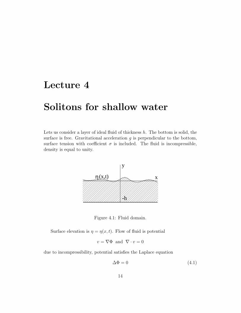
Lets us consider a layer of ideal fluid of thickness h. The bottom is solid, thesurface is free. Gravitational acceleration g is perpendicular to the bottom,surface tension with coefficient σ is included. The fluid is incompressible,density is equal to unity.
-h
x
y
(x,t)η
Figure 4.1: Fluid domain.
Surface elevation is η = η(x, t). Flow of fluid is potential
v = ∇Φ and ∇ · v = 0
due to incompressibility, potential satisfies the Laplace equation
∆Φ = 0 (4.1)
14
Let us denoteΦ|y=η = Ψ(x, t) (4.2)
apparently∂Φ
∂y
∣
∣
∣
∣
y=−h
= 0 (4.3)
Boundary conditions (4.2), (4.3) define uniquely a solution of the Laplaceequation. Thus it is enough to follow the evolution of η(x, t), Ψ(x, t)
We will not prove following theorem.(The proof is put in application.)
Theorem 1
η, Ψ is a pair of canonical variables They obey equations
∂η
∂t=δH
δΨ∂Ψ
∂t= −δH
δη(4.4)
here H – total energy of fluid, consisting of kinetic and potential energy
H = T + U (4.5)
Potential energy can be found in explicit form
U =1
2g
∫ ∞
∞
η2dx+ σ
∫
(√
1 + η2x − 1)dx (4.6)
Kinetic energy is given by formula
T = +1
2
∫ η
−h
∫ +∞
−∞
(∇Φ)2 dydx = −1
2
∫
Ψ · Ψnds (4.7)
Here Ψn is normal derivative of potential.
Ψn =
∫
G(s, s′)Ψ(s′)ds′ (4.8)
Here G(s, s′) = G(s′, s) – Green’s function for the Dirichlet-Neumann bound-ary problem. It cannot be expressed in an explicit form for arbitrary η(x, t).
15
However, the Laplace equation can be solved approximately if kη → 0, k –characteristic wave number.
∆Φ =∂2Φ
∂x2+∂2Φ
∂y2= 0
Φ = Φ0 + Φ1 + . . .
∂2Φ0
∂y2= 0 (4.9)
Φ0 = Ψ(x, t)
∂2Φ1
∂y2= −∂
2Ψ
∂x2(4.10)
Φ1|y=η = 0∂Φ1
∂y
∣
∣
∣
∣
y=−h
= 0
Φ1 = −1
2
∂2Ψ
∂x2· y2 + C1y + C2
−1
2
∂2Ψ
∂x2η2 + C1η + C2 = 0
C1 = −h∂2Ψ
∂x2
C2 =∂2Ψ
∂x2
(
−1
2η2 − hη
)
Assuming that steepness of the surface is small kη → 0, one can put C2 = 0because we need only derivatives of Φ.
Thus
Φ1 = −∂2Ψ
∂x2
(
1
2y2 + hy
)
∂Φ
∂x≃ ∂Ψ
∂x−(
1
2y2 + hy
)
∂3Ψ
∂x3
∂Φ
∂y≃ −∂
2Ψ
∂x2(h+ y)
(
∂Φ
∂x
)2
≃(
∂Ψ
∂x
)2
− 2∂Ψ
∂x
∂3Ψ
∂x3
(
1
2y2 + hy
)
≃
≃(
∂Ψ
∂x
)2
+ 2
(
∂2Ψ
∂x2
)2(
+1
2y2 + hy
)
16
∫ η
−h
[
y2 + 2hy + (h+ y)2]
dy =
=
∫ η
−h
h2 + 4hy + 2y2
dy =
= h2(η + h) + 2hy2∣
∣
η
−h+
2
3y3
∣
∣
∣
∣
η
−h
=
= h2η + 2hη2 +2
3η3 + h3 − 2h3 +
2
3h3 =
= h2η + 2hη2 +2
3η3 − 1
3h3.
Finally
T =1
2
∫(
∂Ψ
∂x
)2
(η + h)dx+
+
∫[
h2η
(
1 + 2η
h+
2
3
η2
h2
)
− 1
6h3
](
∂2Ψ
∂x2
)2
dx (4.11)
U ≃ 1
2g
∫
η2dx+σ
2
∫ (
∂η
∂x
)2
dx
Using weakly nonlinear approximation η << h and kη → 0 one can get
∂η
∂t+
∂
∂x(η + h)
∂2Ψ
∂x2=
1
3h3∂
4Ψ
∂x4
∂Ψ
∂t+
1
2
(
∂Ψ
∂x
)2
+ gη = −σ∂2η
∂x2
(4.12)
This is a system of type (2.1),(2.2)
In the linear approximation
−iωη − hk2
(
1 − 1
3h2k2
)
Ψ = 0
−iωΨ +(
g + σk2)
η = 0
ω2 = ghk2
(
1 − 1
3h2k2
)(
1 +σ
gk2
)
17
σ
g>
1
3h2 – positive dispersion
σ
g<
1
3h2 – negative dispersion
We will show that system (4.12) at σ = 0 is integrable.
18
Lecture 5
Lax representation
Let us consider the following overdetermined system of differential equations
∂Ψ
∂y+ LΨ = 0 (5.1)
∂Ψ
∂t+ AΨ = 0 (5.2)
LΨ =∂2Ψ
∂x2+ UΨ
AΨ = 4∂3Ψ
∂x3+ V
∂Ψ
∂x+WΨ (5.3)
Comparing cross-derivatives ∂2Ψ∂t∂y
= ∂2Ψ∂y∂t
one obtains
(
∂L
∂t− ∂A
∂y−[
L, A]
)
Ψ = 0 (5.4)
System (5.1),(5.2) must be compatible – what does that mean? We demandthat the common Cauchy problem for equations (5.1),(5.2)
Ψ|t=0, y=0 = Ψ0(x) −∞ < x <∞
has at least local solution in some domain on the (y, t) plane for any arbitrary(smooth enough) function Ψ0 of one variable x.
19
Now we observe that operator T = ∂L
∂t− ∂A
∂y−[
L, A]
is an ordinary dif-
ferential operator, annihilating any arbitrary function of one variable. Hencewe can cancel Ψ in (5.4) and require:
∂L
∂t− ∂A
∂y−[
L, A]
= 0 (5.5)
Commutator[
L, A]
is a second-order differential operator identically
equal to zero. Hence, one can “cancel” Ψ in (5.4)
∂L
∂t− ∂A
∂y=[
L, A]
(5.6)
[
L, A]
=
(
2∂V
∂x− 12
∂U
∂x
)
∂2
∂x2+
(
∂2V
∂x2− 12
∂2U
∂x2+ 2
∂W
∂x
)
∂
∂x+∂2W
∂x2− 4
∂3U
∂x3− V
∂U
∂x(5.7)
Condition (5.5) implies
2∂V
∂x− 12
∂U
∂x= 0
V = 6U + C (5.8)
Then
−∂V∂y
=∂2V
∂x2− 12
∂2U
∂x2+ 2
∂W
∂x
∂U
∂t− ∂W
∂y=∂2W
∂x2− 4
∂3U
∂x3− V
∂U
∂x(5.9)
Let us put
W = 3∂V
∂x+ q.
System (5.9) reads now
3∂U
∂y= −∂q
∂x
∂U
∂t+ C
∂U
∂x+∂3U
∂x3+ 6U
∂U
∂x=∂q
∂y(5.10)
20
It is equivalent to the KP-2 equation
∂
∂x
(
∂U
∂t+ C
∂U
∂x+∂3U
∂x3+ 6U
∂U
∂x
)
= −3∂2U
∂y2(5.11)
(the only difference is the coefficient 3 which can be excluded by the trivialrescaling of y)
We found that equation (5.11) is a compatibility condition for followingpair of a linear PDE
±∂Ψ∂y
+∂2Ψ
∂x2+ UΨ = 0
∂Ψ
∂t+ 4
∂3Ψ
∂x3+ C
∂Ψ
∂x+ 6U
∂Ψ
∂x+ (3
∂U
∂x+ q)Ψ = 0 (5.12)
This overdetermined system is the “LAX Pair” for KP-2 equation. Replacing∂∂y
→ − ∂∂y
does not change anything. Let us consider following Lax Pair
±i∂Ψ∂y
+∂2Ψ
∂x2+ UΨ = 0
∂Ψ
∂t+ 4
∂3Ψ
∂x3+ C
∂Ψ
∂x+ 6U
∂Ψ
∂x+ (3
∂U
∂x+ iq)Ψ = 0 (5.13)
Here U , q are real functions. A compatibility condition for (5.13) is equation
∂
∂x
(
∂U
∂t+ C
∂U
∂x+∂3U
∂x3+ 6U
∂U
∂x
)
= 3∂2U
∂y2(5.14)
which can be transformed to KP-1 by already mentioned transform t→ −t,U → −U . Note that both equations (5.11), (5.14) have bump-type solitons.
If there is no dependence on y, one can put Ψ ∼ e−λy and system (5.1),(5.2) goes to following:
Lφ = λφ∂φ
∂t+ Aφ = 0 (5.15)
Now q = 0 and
AΨ = 4∂3Ψ
∂x3+ 6U
∂Ψ
∂x+ 3
∂U
∂xΨ
21
(we put C = 0.) This is the “classical” Lax Pair for KdV equation, whichnow can be written as follows:
∂L
∂t=[
L, A]
(5.16)
For the Boussinesq equation one has the system
AΨ = λΨ
µ∂Ψ
∂y= LΨ
µ2 = ±1
AΨ = 4∂3Ψ
∂x3+ 6U
∂Ψ
∂x+ 3
∂U
∂xΨ + µqΨ + C
∂Ψ
∂x(5.17)
Here C = ±1
Aditional remarks
1) One can assume that U is complex and study the complex KdV
∂U
∂t+ U
∂U
∂x+ a
∂3U
∂x3= 0 (5.18)
where a – any complex number.
Suppose that U = ∂Φ∂x
+ iρ, a = iα. Now equation (5.18) is equivalent tothe system
∂ρ
∂t+
∂
∂xρ∂Φ
∂x= −α∂
3Φ
∂x3
∂Φ
∂t+
1
2
(
∂Φ
∂x
)2
− 1
2ρ2 = α
∂2ρ
∂x2(5.19)
This is a badly unstable system with Hamiltonian
H =1
2
∫
ρ
(
∂Φ
∂x
)2
dx− 1
6
∫
ρ3dx− α
2
∫(
∂2Φ
∂x2
)2
+α
2
∫(
∂ρ
∂x
)2
(5.20)
2) One can assume that U , V , W are matrix functions. In this case onegets matrix generalizations of KdV, KP and Boussinesq equations. The mostsimple is the matrix KdV equation
∂U
∂t+ 3
∂
∂xU2 +
∂3U
∂x3= 0 (5.21)
22

Here U — any N×N matrix. One can assume that U is symmetric: UT = U
Homework
Construct matrix generalisation of the KP-equation.
23
Lecture 6
From KdV to NLSE
Let us study again overdetermined compatible pair of equations
∂χ
∂y+ Lχ = 0 (6.1)
∂χ
∂t+ Aχ = 0 (6.2)
where again
L =∂2
∂x2+ u
A = 4∂3
∂x3+ (6u+ c)
∂
∂x+ 3
∂u
∂x+ q
But now χ is vector in Cn χ =
x1...xn
while u, q are n× n matrix functions
on x, t, y, and c = c(t) is a matrix function on t only. One can easily checkthat equation
∂L
∂t− ∂A
∂y=[
L, A]
(6.3)
takes the following form
∂q
∂x= −3
∂u
∂y+
1
2[c, u] (6.4)
∂u
∂t+
1
2
(
c∂u
∂x+∂u
∂xc
)
+ 3∂
∂xu2 +
∂3u
∂x3=∂q
∂y+ [u, q] (6.5)
24
This system is a matrix version of the KP equation. We study first one-dimensional case ∂u/∂y = 0, ∂q/∂y = 0 and assume that c is a scalar. Nowequation (6.5) reads
∂u
∂t+ c
∂u
∂x+ 3
∂
∂xu2 +
∂3u
∂x3+ [q, u] = 0 (6.6)
q = q(t) - arbitrary matrix function on time. Equation (6.6) is a matrixversion on the KdV equation.
Let n = 2
u =
[
A ψ±ψ A
]
q =iλ
2
[
1 00 −1
]
(6.7)
Now (6.6) is equivalent to following pair of equations.
∂A∂t
+ c∂A∂x
+ 3∂
∂x
(
A2 ± |ψ|2)
+∂3A∂x3
= 0 (6.8)
∂ψ
∂t+ c
∂ψ
∂x+ 6
∂
∂xAψ + iλψ +
∂3ψ
∂x3= 0 (6.9)
We will show that system (6.8), (6.9) generates well-known Nonlinear Schrodingerequation Let k > 0 – some real number. We choose
c = 3k2 λ = −2k3
and introduce new time variable
τ = kt
and new unknown function
ϕ =1
ke−ikxψ ψ = keikxϕ (6.10)
now system (6.8) (6.9) turns to following
∂
∂x
(
A± |ϕ|2)
= − 1
3k
∂A∂τ
− 1
3k2
(
∂3A∂x3
+ 3∂
∂xA2
)
∂ϕ
∂τ+ i
(
∂2ϕ
∂x2+ 6Aϕ
)
+1
k
(
6∂
∂xAϕ+
∂3ϕ
∂x3
)
= 0 (6.11)
25
Now let k → ∞. We set
∂
∂x
(
A± |ϕ|2)
= 0
∂ϕ
∂τ+ i
(
3∂2ϕ
∂x2+ 6Aϕ
)
= 0
using simple scaling τ → τ/6, x→ x/√
2 one can get
∂ϕ
∂τ+ i
(
∂2ϕ
∂x2∓ |ϕ|2ϕ+ ω(t)ϕ
)
= 0 (6.12)
(6.12) is the Nonlinear Schrodinger Equation (NLSE). Linear term ω(t) can
be excluded by multiplication by factor e−i
R t
t0ω(t′)dt′
. Equation
∂ϕ
∂τ+ i
(
∂2ϕ
∂x2− |ϕ|2ϕ
)
= 0 (6.13)
is defocusing NLSE. Equation
∂ϕ
∂τ+ i
(
∂2ϕ
∂x2+ |ϕ|2ϕ
)
= 0 (6.14)
is focusing NLSE.
Let us use a substitution χ→ χe−λy in (6.1). In the absence of coefficientdependence on y , the equation turns to
Lχ = λχ, where χ =
[
χ1
χ2
]
∂2χ1
∂x2+ Aχ1 + ψχ2 = λχ1
∂2χ2
∂x2± ψχ1 + Aχ2 = λχ2 (6.15)
We will assume
χ1 = ξ1eikx2 χ2 = ξ2e
− ikx2
λ = −k2
4+ kµ (6.16)
26
Equation (6.15) can be written as follows:
i∂ξ1∂x
+ φξ2 − µξ1 = −1
k
(
∂2ξ1∂x2
+ Aξ1)
−i∂ξ2∂x
± φξ1 − µξ2 = −1
k
(
∂2ξ2∂x2
+ Aξ1)
(6.17)
Equation (6.2) in the vector case reads
k∂χ1
∂τ+ 4
∂3χ1
∂x3+ 3
(
k2 + 2A) ∂χ1
∂x+ 6ψ
∂χ2
∂x
+
(
3∂A∂x
− ik3
)
χ1 + 3ψxχ2 = 0
k∂χ2
∂τ+ 4
∂3χ2
∂x3+ 3
(
k2 + 2A) ∂χ2
∂x± 6ψ
∂χ1
∂x
+
(
3∂A∂x
+ ik3
)
χ2 ± 3ψxχ1 = 0 (6.18)
Plugging (6.16) in (6.18) after few simple transformations one gets
∂ξ1∂τ
+ 6i∂2ξ1∂x2
+ 6ϕ∂ξ2∂x
+ 3iAξ1 + 3∂ϕ
∂xξ2 =
−1
k
(
4∂3ξ1∂x3
+ 6A∂ξ1∂x
+ 3∂A∂x
ξ1
)
∂ξ2∂τ
− 6i∂2ξ2∂x2
± 6ϕ∂ξ1∂x
− 3iAξ2 ± 3∂ϕ
∂xξ1 =
−1
k
(
4∂3ξ2∂x3
+ 6A∂ξ2∂x
+ 3∂A∂x
ξ1
)
(6.19)
Now one can make the limiting transition k → ∞ and set the followingequation
i
[
1 00 −1
]
∂ξ
∂x+
[
0 ϕ±ϕ 0
]
ξ = µξ
∂ξ
∂τ+ 6i
[
1 00 −1
]
∂2ξ
∂x2+ 6
[
0 ϕ±ϕ 0
]
∂ξ
∂x
+3
[
iA ∂ϕ∂x
±∂ϕ∂x
iA
]
ξ = 0 (6.20)
ξ =
[
ξ1ξ2
]
27
Thus for the NLSE
L = i
[
1 00 −1
]
∂
∂x+
[
0 ϕ±ϕ 0
]
(6.21)
for defocusing NLSE it is self-adjoint operator, for focusing NLSE it is nonself-adjoint.
A = 6i
[
1 00 −1
]
∂2
∂x2+ 6
[
0 ϕ±ϕ 0
]
∂
∂x+ 3
[
iA ∂ϕ∂x
±∂ϕ∂x
−iA
]
(6.22)
28
Lecture 7
From KP to DS - multiscale
expansion
In this chapter we will start with scalar KP2 equation
∂
∂x
(
∂u
∂t+ 3k2∂u
∂x+∂3u
∂x3+ 3
∂
∂xu2
)
+ 3∂2u
∂y2= 0 (7.1)
Here k is some constant. We will not use limiting transition k → ∞. Insteadwe will use multiscale expansion.
We present solution of (7.1) in a form
u =ε
2
(
ΨeiΦ + Ψe−iΦ)
+ ε2
(
u0 +1
2Ψ2e
2iΦ +1
2Ψ2e
−2iΦ
)
(7.2)
here ε – small parameter, Φ = −2k3t+ kx
In (7.2) Ψ, u0, Ψ2 are functions of slow variables τ = ε2t, ξ = εx, η = εy.Plugging (7.2) into (7.1), one can see that terms of order ε are cancelled.After substituting (7.2) to (7.1) we have to cancel terms proportional toe±inΦ separately.
In equation for n = 0, n = 2 leading order terms are proportional to ε2.Putting n = 0, one obtains equation
(
k2 ∂2
∂ξ2+
∂2
∂η2
)
u0 = −1
2
∂2
∂ξ2|Ψ|2 (7.3)
29
Amplitude of second harmonic Ψ2 can be found in explicit form
1
2
[
2i∂Φ
∂t+ 3k2 · 2i∂Φ
∂x+
(
2i∂Φ
∂x
)3]
Ψ2 +3 · 2iΦx
4Ψ2 = 0 (7.4)
∂Φ
∂t= −2k3 ∂Φ
∂x= k
From (7.4) one obtains
Ψ2 =1
2k2Ψ2 (7.5)
In equation for first harmonic n = 1 first nonvanishing term is proportionalto ε4. Collecting all these terms together we obtain the equation
ik∂Ψ
∂τ+ 3
(
−k2 ∂2
∂ξ2+
∂2
∂η2
)
Ψ − 6k2
(
u0Ψ +1
2Ψ2Ψ
)
= 0
taking Ψ2 from (7.5) we set
ik∂Ψ
∂τ+ 3
(
−k2 ∂2
∂ξ2+
∂2
∂η2
)
Ψ − 6k2
(
u0Ψ +1
4k2|Ψ|2Ψ
)
= 0 (7.6)
System (7.3), (7.6) is known as Davey-Stewanson equation.
It is remarkable that sign before second spatial derivative k2 ∂2
∂ξ2 in equa-
tion (7.3) and (7.6) are opposite. Transition from KP2 to KP1 equation isperformed by change ∂
∂η→ i ∂
∂η, ∂2
∂η2 → − ∂2
∂η2 . If we would start from KP1equation we should make this replacement. Now the system takes form
(
k2 ∂2
∂ξ2− ∂2
∂η2
)
u0 = −1
2
∂2
∂ξ2|Ψ2|
ik∂Ψ
∂τ− 3
(
k2 ∂2
∂ξ2+
∂2
∂η2
)
Ψ − 6k2
(
u0Ψ +1
4k2|Ψ|2Ψ
)
= 0 (7.7)
Equation (7.3)-(7.6) have a remarkable special solutions. Suppose that
∂
∂η= α
∂
∂ξ
In other words, a solution depends only on ξ + αη
30
Now equation (7.3) can be integrated
u0 = −1
2
1
k2 + α2|Ψ|2
u0 +1
4k2|Ψ|2 = − k2 − α2
4k2(k2 + α2)|Ψ|2
Equation (7.6) now takes form
ik∂Ψ
∂τ− 3(k2 − α2)
[
∂2Ψ
∂ξ2− 1
2
1
k2 + α2|Ψ|2Ψ
]
= 0 (7.8)
For any α it is the defocusing Nonlinear Schrodinger equation.
If we start from KP-1 equation, α2 should be replaced by −α2, and equa-tion (7.8) reads
ik∂Ψ
∂τ− 3(k2 + α2)
[
∂2Ψ
∂ξ2− 1
2
1
k2 − α2|Ψ|2Ψ
]
= 0 (7.9)
If α2 > k2, this is focusing NLSE.
Now one can address the question — what is going on with Lax pairs inprocess of multiscale expansion. Equation
∂χ
∂y+ Lχ = 0
∂χ
∂y+∂2χ
∂x2+ε
2
(
Ψeikx + Ψe−ikx + . . .)
χ = 0 (7.10)
Equation (7.10) is a scalar equation, to turn it to the vector equation, onecan find the wave function χ in following form
χ =(
χ1eikx2 + χ−1e
−ikx2 + ...
)
ek2y
4 (7.11)
Equation (7.10) has to be expanded in Fourier series
χ =
∞∑
n=1
χneinkx
2
Taking into account only major terms one get following system of equations:
∂χ1
∂y+ ik ∂χ1
∂x+ 1
2Ψχ−1 = 0
∂χ1
∂y− ik ∂χ1
∂x+ 1
2Ψχ1 = 0
(7.12)
31
Equation
∂χ
∂t+ 4
∂3χ
∂x3+(
6u+ 3k2) ∂χ
∂x+
(
3∂u
∂x+ q
)
χ = 0 (7.13)
∂q
∂x= −3
∂u
∂y
also can be transformed to a system of equations for χ1, χ−1. To do this, weagain present χ in form (7.11) and use expansion (7.2). We realize that firstnon-vanishing terms are of order ε2. Collecting them together one see thatequation (7.13) is now a system
∂χ1
∂τ+ 6ik
∂2χ1
∂ξ2+ 3Ψ
∂χ−1
∂ξ+ 3iku0χ1 +
3
2
∂Ψ
∂ξχ−1 = 0
∂χ2
∂τ− 6ik
∂2χ−1
∂ξ2+ 3Ψ
∂χ1
∂ξ− 3iku0χ−1 +
3
2
∂Ψ
∂ξχ1 = 0 (7.14)
(7.15)
L = ik
(
1 00 −1
)
∂
∂ξ+
1
2
(
0 ΨΨ 0
)
A = 6ik
(
1 00 −1
)
∂2
∂ξ2+ 3
(
0 ΨΨ 0
)
∂
∂ξ+
3
2
(
2iku0∂Ψ∂ξ
∂Ψ∂ξ
−2iku0
)
(7.16)
32
Lecture 8
Hamiltonian formalism for
waves in weakly nonlinear
media
We study a medium described by one pair of canonical variables ρ,Φ
∂ρ
∂t=δH
δΦ
∂Φ
∂t= −δH
δρ(8.1)
The Hamiltonian H is some functional on ρ,Φ. Let us perform Fouriertransform
Φ(~r) =1
(2π)d/2
∫
Φ(~k)ei~k~rd~k; ρ(~r) =1
(2π)d/2
∫
ρ(~k)ei~k~rd~k
Φ(~k) =1
(2π)d/2
∫
Φ(~r)e−i~k~rd~r; ρ(~k) =1
(2π)d/2
∫
ρ(~r)e−i~k~rd~r(8.2)
From now on during the next three lectures we will ommit the vector-signof ~k, ~q and ~r. After Fourier transform
∂ρ(k)
∂t=
1
(2π)d/2
∫
e−ikr δH
δΦdr
δH
δΦ(r)=
∫
δH
δΦ(q)
δΦ(q)
δΦ(r)dq
33
δΦ(q)
δΦ(r)=
1
(2π)d/2e−iqr (8.3)
HenceδH
δΦ(r)=
1
(2π)d/2
∫
δH
δΦ(q)e−iqrdq
Thus∂ρ(k)
∂t=
1
(2π)d
∫
e−i(k+q,r) δH
δΦ(q)drdq
However1
(2π)d
∫
e−i(k+q,r)dr = δ(k + q) (8.4)
Finally∂ρ(k)
∂t=
δH
δΦ(−k)But Φ(−k) = Φ(k), ρ(−k) = ρ(k) After Fourier transform equation (8.1)take from
∂ρ
∂t=
δH
δΦ(k)
∂Φ(k)
∂t= − δH
δρ(k)(8.5)
For beginning we suppose that the Hamiltonian H is quadratic functionalinvariant with respect to spatial transitions. The most general form of suchfunctional is following
H =1
2
∫
A(k)Φ(k)Φ(k)dk +1
2
∫
B(k)ρ(k)Φ(k)dk +
+1
2
∫
B′(k)ρ(k)Φ(k)dk +1
2
∫
C(k)ρ(k)ρ(k)dk (8.6)
H is a real functional, hence
A(−k) = A(k) = A(k)
C(−k) = C(k) = C(k) (8.7)
B(k) = B′(k)
34
B(−k) = B′(k) this means
B(k) = B1 + iB2(k)
B1(−k) = B1(k) (8.8)
B2(−k) = −B2(k)
Equations (8.5) now are
∂ρ
∂t= AΦ + (B1 + iB2)ρ
∂Φ
∂t= (−B1 + iB2)Φ − Cρ (8.9)
Assuming that ρ,Φ ∼ eiωt one obtains
ω(k) = B2 ± ∆ ∆ =√
AC − B21 (8.10)
The medium is stable if AC − B21 > 0. In virtue of (8.7) (8.8)
∆(−k) = ∆(k)
Thus ∆(k) and B2(k) are symmetric and antisymmetric parts of frequency.Equation for ω(k) has two solutions, but only one of them has physicalmeaning. To determine the sign in (8.10), we have to introduce normal
variables
a(k) = u(k)ρ(k) + v(k)Φ(k) (8.11)
Such that∂a(k)
∂t= iω(k)a(k) (8.12)
sign in ω(k) is still not known. Plugging (8.11) to (8.12) and using equation(8.9) one gets
(iω + (B))v = uA
u =1
A(B1 ± i∆)v
we assume v(−k) = v(k) = v(k). Thus
a(k) = v
[
Φ +1
A(B1 ± i∆)ρ
]
a∗(−k) = v
[
Φ +1
A(B1 ∓ i∆)ρ
]
(8.13)
35
Then
ρ = ∓ iA
2v∆(a(k) − a∗(−k)) (8.14)
Φ =1
2v(a(k) + a∗(k)) − B1
Aρ = (8.15)
=1
2v
[(
1 ± iB1
∆
)
a(k) +
(
1 ∓ iB1
∆
)
a∗(−k)]
To determine v(k) we substitute (8.15), (8.14) to the Hamiltonian and de-mand that
H =
∫
ω(k)a(k)a(k)dk (8.16)
A relatively long calculation leads to a very simple result
v2 = ± A
2∆(8.17)
or
v =|A| 12√
2∆(8.18)
obviously sign in (8.17) should coincide with the sign of A. Finally
ω(k) = B2(k) + signA(k) · ∆(k)
Sign of ω(k) has clear physical meaning – Waves with wave vector ~k havepositive energy if ω(k) > 0 and negative energy in the opposite case.
For normal variable one gets
ρ = −isignA|A|1/2
√2∆1/2
(a(k) − a∗(−k))
Φ =∆1/2
√
2|A|
[(
1 ± iB1
∆
)
a(k) +
(
1 ∓ iB1
∆
)
a∗(−k)]
(8.19)
Comment
In nonlinear media the Hamiltonian cannot be transformed to form (8.16).
In a weakly nonlinear medium the Hamiltonian can be expanded in termsof canonical variables.
H = H2 +H3 +H4 . . . (8.20)
36
One can perform this expansion in normal variables. Now
H2 =
∫
ω(k)a(k)a∗(k)dk
H3 = H(1)3 +H
(2)3
H(1)3 =
1
3!
∫
V(0,3)k,k1,k2
akak1ak2 + c.c.
δ(k + k1 + k2)dk dk1 dk2 (8.21)
H(2)3 =
1
1!2!
∫
V(1,2)k,k1,k2
a∗kak1ak2 + c.c.
δ(k − k1 − k2)dk dk1 dk2 = H1,2
The whole Hamiltonian can be presented as a sum
H =∑
n,m
Hn,m n ≤ m
Hn,m =1
n!m!
Vk1...kn,kn+1...kn+ma∗(k1) . . . a
∗(kn)a(kn+1) . . . a(kn+m) + +c.c.
××δ(k1 + . . .+ kn − kn+1 − . . .− kn+m)dk1 . . . dkn+m
37
Lecture 9
Three waves interactions
In the last chapter we introduced normal variable ak
ak = ukρk + vkΦk (9.1)
and defined coefficients uk, vk from two conditions:
1. ak satisfies the equations
∂ak
∂t= iωkak (9.2)
2. Quadratic Hamiltonian H2 (8.16) has diagonal form
H2 =
∫
ωkaka∗kdk
Now equation (9.2) can be presented as follows
∂ak
∂t= i
δH
δa∗k(9.3)
Now we address following question. Let H is an arbitrary Hamiltonian.What condition we have to impose on u, v to provide validity of equation(9.3)?
From (9.1) one obtains
38
a∗k = u∗kρ∗k + v∗kΦ
∗k
a−k = u−kρ∗k + v−kΦ
∗k
(9.4)
Then, after differentiation of (9.3) by time
∂ak
∂t= uk
∂ρk
∂t+ vk
∂Φk
∂t
iδH
δa∗k= uk
δH
δΦ∗k
− vkδH
δρ∗k(9.5)
δH
δρ∗k=δH
δa∗k
δa∗kδρ∗k
+δH
δa−k
δa−k
δρ∗k= u∗k
δH
δa∗k+ u−k
δH
δa−k
(9.6)
In the same wayδH
δΦ∗k
= v∗kδH
δa∗k+ v−k
δH
δa−k
(9.7)
Substituting (9.6), (9.7) to (9.5) and assuming that condition (9.3) issatisfied for any Hamiltonian H , one gets
iδH
δa∗k= uk(v
∗k
δH
δa∗k+ v−k
δH
δa−k) − vk(u
∗k
δH
δa∗k+ u−k
δH
δa−k) (9.8)
Condition (9.8) must be valid for any Hamiltonian H . It implies followingcondition on coefficients
ukv−k = u−kvk (9.9)
ukv∗k − vku
∗k = i (9.10)
In previous chapter we found
uk =1
A(B1 ± i∆)vk v2
k = ± A
2∆(9.11)
Substituting (9.11 into (9.9), (9.10) one can see that these conditions aresatisfied.
39
We have proved a very important theorem - change of variables (8.19)transforms any Hamiltonian equation (8.1) to equation (9.3).
Suppose that Hamiltonian H is expanded in series in powers of aka∗k.
We assume that the medium is homogeneous. It means that Hamiltonianshould be invariant with respect to transform ak → ake
i(k,λ) where λ-arbitraryvector. The Hamiltonian is
H = H2 +H3 + . . .
H2 =
∫
ωk|ak|2dk
H3 = H(1)3 +H
(2)3
H(1)3 =
1
6
∫
V (0,3)k,k1,k2
akak1ak2 + V∗(0,3)k,k1,k2
a∗ka∗k1a∗k2
δ(k − k1 − k2)dkdk1dk2(9.12)
H(2)3 =
1
2
∫
V (1,2)k,k1,k2
a∗kak1ak2 + V∗(1,2)k,k1,k2
aka∗k1a∗k2
δ(k − k1 − k2)dkdk1dk2(9.13)
Equations (9.3) are following
∂ak
∂t= iωkak + i
∫
1
2V
∗(0,3)k,k1,k2
a∗k1a∗k2δ(k + k1 + k2)+
+1
2V
(1,2)k,k1,k2
ak1ak2δ(k − k1 − k2) + V∗(1,2)k,k1,k2
a∗k1ak2δ(k + k1 − k2)
dk1dk2(9.14)
Note that in a general case the Hamiltonian H can be presented as follows
H =∑
n,m
Hn,m n ≤ m
Hnm =1
n!m!
∫
V (n,m)k1,...knkn+1...kn+m
ak1 . . . akna∗kn+1 . . . a
∗kn+mδ(k1 +
+ . . . kn − kn+1 . . .− kn+m) + . . .dk1 . . . dkn+m (9.15)
Suppose now that ω(k) ≥ 0 and
ω(k1 + k2) = ω(k1) + ω(k2) (9.16)
40
has nontrivial solutions. In the simplest case, when dimension of the spaced ≥ 2 and ω′(k) > 0 ω = ω(|k|) one can find a sufficient condition forsolvability of equation (9.16). This condition is positivity of dispersion ω′′ >0. Indeed, in this case, for parallel vectors k1, k2
ω(k1 + k2) > ω(k1) + ω(k2) (9.17)
Now replacing k1 → k1 + k⊥, k2 → k2 − k⊥ where (k⊥, k1) = 0, one canturn inequality (9.17) to equality.
Suppose we found three wave vectors p1, p2, p3 comprising the resonanttriad
p1 = p2 + p3
ω(p1) = ω(p2) + ω(p3)(9.18)
Let the wave filed a(k) is a combination of three quasi-monochromaticwave trains
a(k) = A(k) +B(k) + C(k) (9.19)
We assume that A(k) = 0 if |k − p1| > ǫ, B(k) = 0 if |k − p2| > ǫ,C(k) = 0 if |k − p3| > ǫ. Here ǫ is a small parameter. Functions A,B,C areconcentrated near wave vectors p1, p2, p3.
To construct approximate envelope equations we perform change of vari-ables
ak = eiωktck (9.20)
From (9.14) we obtain
∂ck∂t
= i
∫
1
2V
∗(0,3)k,k1,k2
c∗k1c∗k2e−i(ωk+ωk1
+ωk2)tδ(k + k1 + k2) +
+1
2v
(1,2)k,k1,k2
ck1ck2e−i(ωk−ωk1
−ωk2)tδ(k − k1 − k2) + (9.21)
+V∗(1,2)k,k1,k2
c∗k1ck2e
−i(ωk+ωk1−ωk2
)tδ(k + k1 − k2)dk1dk2 (9.22)
41
Let in (9.20) k is close to p1, ω(k) -close to ω(p1). In the right hand sideof (9.21) most terms are fast oscillating. In the limit of small amplitude|ak| → 0 they can be neglected. Only “secular”, non-oscillating terms areimportant. Looking at the right hand side of equation (9.21), one can seethat only second term can be slowly oscillating, if we assume k1 ≃ p2, k2 ≃ p3
or viceversa. Taking into account only these terms and returning back fromck to ak one can put approximately
∂A
∂t= iω(k)Ak + i
∫
V(1,2)k,k1,k2
Bk1Ck2δk−k1−k2dk1dk2 (9.23)
Now one can put
k = p1 + κ k1 = p2 + κ1 k2 = p3 + κ2
and introduce
A = Aeiω(p1)t B = Beiω(p2)t C = Ceiω(p3)t
Then equation (9.23) reads
∂Aκ
∂t= i(ω(p1 +κ)−ω(p1))Ak + i
∫
V(1,2)p1+κ,p2+κ1,p3+κ2
Bκ1Cκ2δκ−κ1−κ2dκ1dκ2
(9.24)Now we can put approximately
ω(p1 + κ) − ω(p1) = (v,κ)
here v1 = ∂ω∂k|k=p1-group velocity of the first wave train A(k) and
V(1,2)p1+κ,p2+κ1,p3+κ2
≃ (2π)−d/2Up1,p2,p3
U is a constant.
Now from (9.24) one obtains
A
δt= i(κv1))Aκ
+ i(2π)−d/2U
∫
Bκ1Cκ2δ(κ − κ1 − κ2)dκ1dκ2
42
Performing Fourier transform
a(r) =1
(2π)d/2
∫
A(κ)eiκrdκ
A(κ) =1
(2π)d/2
∫
a(r)e−iκrdr
and similar transforms for B, C, one ends up with following PDE
∂a
∂t+ (v1∇)a = iubc
Repeating this procedure, assuming k ≃ p2 and k ≃ p3, we get finallyfollowing system of nonlinear PDE
∂a
∂t+ (v1∇)a = iubc
∂b
∂t+ (v2∇)b = iu∗ac∗
∂c
∂t+ (v3∇)c = iu∗ab∗
(9.25)
here
v2 =∂ω
∂k|k=p2 v3 =
∂ω
∂k|k=p3
In these equations u is a complex constant.
u = (2π)d/2V (1,2)p1,p2,p3
= |u|eiφ
By simple transform
a→ |u|−1/2e−iφa b→ |u|−1/2e−iφb c→ |u|−1/2e−iφc
one can put u = 1 and finally get the system
∂a
∂t+ (v1∇)a = ibc
∂b
∂t+ (v2∇)b = iac∗
∂c
∂t+ (v3∇)c = iab∗
(9.26)
43
This is so-called “three-wave system”. This system admits following re-duction
a = iu b = iv c = iw
where u, v, w -are real functions. Now
∂u
∂t+ (v1∇)u = −vw∂v
∂t+ (v2∇)v = uw
∂w
∂t+ (v3∇)w = uv
(9.27)
In the spatial homogenous case this system simplifies to the system ofODE’s
∂u
∂t= −vw
∂v
∂t= uw
∂w
∂t= uv
(9.28)
identical to the Euler equation for free rotation of three-dimensional rigidbody.
Spatially homogenous system (9.26) reads
∂a
∂t= ibc
∂b
∂t= iac∗
∂c
∂t= iab∗
(9.29)
This system has following constant of motion
44
|a|2 + |b|2 = I1
|a|2 + |c|2 = I2(9.30)
In the case of amplitudes tending to zero at boundaries (or in infinity)general system (9.26) has constants of motion
∫
|a|2dr +
∫
|b|2dr = I1∫
|a|2dr +
∫
|c|2dr = I2(9.31)
These motion constants are known as Manley-Row relations.
Now suppose that ω(k) can change sign. In other words, we have bothwaves of positive and negative energy. In such medium one could find a triadsatisfying following conditions
p1 + p2 + p3 = 0
ω(p1) + ω(p2) + ω(p3) = 0(9.32)
For these triads the main nonlinear term is H(1)3 . Repeating previous
considerations one ends up with the system
∂a
∂t+ (v1∇)a = −ib∗c∗
∂b
∂t+ (v2∇)b = −ia∗c∗
∂c
∂t+ (v3∇)c = −ia∗b∗
(9.33)
The Manley-Row relations now take form
45
∫
|a|2dr −∫
|b|2dr = I1∫
|a|2dr −∫
|c|2dr = I2(9.34)
System (9.33) has a simple solution
a = b = c = −iu∂u
∂t= u2
u =1
t0 − t
(9.35)
This equation describes spatially uniform explosion (collapse).
46
Lecture 10
From KP-1 Equation to 3-wave
System
In this lecture we will derive the 3-wave system from the KP-1 equation andfind Lax pair for 3-wave system. We start from the KP-1 equation
∂
∂x
(
∂u
∂t+ 3
∂u2
∂x+∂3u
∂x3
)
− 3∂2u
∂y2= 0 (10.1)
After Fourier transform
u(x, y) =1
2π
∫
u(p, q)ei(px+qy)dp dq
p, q are components of wave vector k = (p, q) and
u(p, q) =1
2π
∫
u(x, y)e−i(px+qy)dx dy
Equation (10.1) takes form
∂uk
∂t= iω(k)uk −
3ip
2π
∫
uk1uk2δ(k − k1 − k2)dk1 dk2 (10.2)
Let in (10.2) p > 0
As far asu−k = u∗k (10.3)
47
one can transform equation (10.2) to following form
∂u(p, q)
∂t= iω(p, q)u(p, q)− 3ip
2π
∫
p1 > 0p2 > 0
(up1q1up2q2δ(p− p1 − p2)δ(q − q1 − q2)+
+2u∗p1q1up2q2δ(p+ p1 + p2)δ(q + q1 − q2)
)
dp1 dp2 dq1 dq2
Here
ω(p, q) = p3 +3q2
p(10.4)
Now we introduce normal variables
up,q =
√
p
2ap,q
In these variables
∂a(p, q)
∂t= iω(p, q)a(p, q) − 3ip
2π
∫
p1 > 0p2 > 0
(pp1p2)1/2 (up1q1up2q2δ(p− p1 − p2)δ(q − q1 − q2)+(10.5)
+2u∗p1q1up2q2δ(p+ p1 + p2)δ(q + q1 − q2)
)
dp1 dp2 dq1 dq2
One can check directly that equation (10.5) can be written in the form
∂a(p, q)
∂t= i
δH
δa∗p,q
H =
∫
p>0
ω(p, q)|apq|2dp dq −
3
4π
∫
p1 > 0p2 > 0p3 > 0
(p1p2p3)1/2(
u∗p1q1up2q2up3q3 + up1q1u
∗p2q2
u∗p3q3
)
× (10.6)
×δ(p1 − p2 − p3)δ(q1 − q2 − q3)dp1 dq1 dp2 dq2 dp3 dq3
One can easily check that in initial variables the Hamiltonian is
H =1
2
∫
[
u2x + 3
(
∂−1uy
)2]
− u3
dx dy (10.7)
Later on we will show that equation (10.1) has infinite number of motionconstants. They will be discussed in the further lectures. So far we estab-lished that KP-1 equation is a Hamiltonian system belonging to the classdescribed in lecture 9.
48
This could be starting point for derivation of the three-wave system. Firstof all we have to be sure that resonant triads do exist. To see this we notefirst that dispersion relation (10.4) can be parameterized as follows
p = ξ1 − ξ2
q = ±(ξ21 − ξ2
2) (10.8)
ω = 4(ξ31 − ξ3
2)
As far as p > 0 ξ1 > ξ2. Since this time, we will study only the case ξ21 > ξ2
2 ,q > 0 and ξ1, ξ2 are positive. Let us consider the triad
p1 = ξ1 − ξ2 p2 = ξ2 − ξ3 p3 = ξ1 − ξ3q1 = ξ2
1 − ξ22 q2 = ξ2
2 − ξ23 q3 = ξ2
1 − ξ23
ω1 = 4(ξ31 − ξ3
2) ω2 = 4(ξ32 − ξ3
3) ω3 = 4(ξ31 − ξ3
3)(10.9)
Apparently (10.9) comprise the resonant triad
p1 + p2 = p3
q1 + q2 = q3
ω1 + ω2 = ω3
Now we will derive a system, more general then 3-wave.
Let us define ξ1 > ξ2 > . . . > ξn > 0
Φik = (ξi − ξk)x+ (ξ2i − ξ2
k)y + 4(ξ3i − ξ3
k)t (10.10)
Φik + Φkj = Φij Φki = −Φik
Suppose that the wave field u is a composition of quasi-monochromatic wavetrains
u =∑
i,j
εuij(ξ, η)eiΦij i 6= j (10.11)
uji = u∗ijξ = εx η = εy τ = εt
Here ε is a small parameter. Let us look for e−iΦiju2. It has oscillating andnon-oscillating terms. Neglecting oscillating terms, we set
e−iΦiju2 ≃∑
k 6= ik 6= j
ε2uikukj + . . . (10.12)
49
Plugging (10.11) in (10.1) and keeping only terms of order ε2, one obtainsthe following system
∂
∂τuij = (~vij∇)uij − 3i (ξi − ξj)
∑
k 6= ik 6= j
uikukj (10.13)
~vij∇ = v(1)ij
∂
∂ξ+ v
(2)ij
∂
∂η
v(1)ij =
∂
∂pω(p, q) = 3
(
p2 − q2
p2
)
= 12ξiξj (10.14)
v(2)ij =
∂
∂qω(p, q) =
6q
p= 6(ξ1 + ξ2)
In the simplest case n = 3, assuming u13 = (ξ1−ξ3)1/2A, u12 = (ξ1−ξ3)1/2B,u23 = (ξ2 − ξ3)
1/2C one obtains 3-wave system with interaction coefficient
u = −3(ξ1 − ξ2)1/2(ξ1 − ξ3)
1/2(ξ2 − ξ3)1/2
To find Lax pair for system (10.13) we start with the first Lax operator forKP-1
−i∂χ∂y
+∂2χ
∂x2+ uχ = 0 (10.15)
we will seek its solutions in a form
χ =n∑
k=1
χkeiξkx+iξ2
ky+4iξ3
kt (10.16)
χk = χk(ξ, η, τ)
Keeping in (10.15) only non-oscillating terms of order ε, one obtains thesystem
i
(
−∂χj
∂η+ 2ξj
∂χj
∂ξ
)
+∑
k 6=j
ujkχk = 0 (10.17)
Repeating this procedure with the second equation one yields
∂χi
∂τ− 12ξ2
i
∂χi
∂ξ+ 3i
∑
k=
(ξi + ξk)uikχk = 0 (10.18)
One can check that the compatibility conditions for equations (10.17), (10.18)is exactly equation (10.10)
50
System (10.13) is a special class of more general system of n-waves. Toconstruct the general system we start with the following overdetermined pairof linear equations
∂Ψ
∂y= F
∂Ψ
∂x+ [F,Q]Ψ (10.19)
∂Ψ
∂t= G
∂Ψ
∂x+ [G,Q]Ψ (10.20)
Here F , G are commuting matrices: [F,G] = 0. One can think that they arediagonal:
F =
a1 0. . .
0 an
G =
b1 0. . .
0 bn
Compatibility condition for system (10.19), (10.20) is following
∂
∂t[F,Q]− ∂
∂y[F,Q] +F
∂
∂x[G,Q]−G
∂
∂x[F,Q]− [[F,Q], [G,Q]] = 0 (10.21)
One can consider that diagonal elements ofQ are zero. Then equation (10.21)read
(bi − bj)∂Qij
∂y+ (biaj − ajbi)
∂Qi,j
∂x=∑
k 6=i,j
εikjQikQkj (10.22)
εikj = aibk − akbi + ajbi − aibj + akbj − ajbk (10.23)
Let I – some real diagonal matrix I2 = 1. All diagonal elements Ikk = ±1.Suppose that Q satisfies the condition
Q+ = IQI (10.24)
This condition is called reduction.
If n = 3, completely anti-symmetric tensor εikj has only one componentε = ε123. Let us assume that I = 1, a1 > a2 > a3
Q13 =i√
a1 − a3
A
Q12 =i√
a1 − a2
B (10.25)
Q23 =i√
a2 − a3
C
Qij = −iQ∗ji
51
We go to the three wave system
V(1)ij =
ajbi − aibjai − aj
V(2)ij =
bi − bjai − aj
u =ε123
√
(a1 − a2)(a1 − a3)(a2 − a3)
Assuming that
I =
1 0 00 −1 00 0 1
Q13 =iA∗
√a1 − a3
Q12 =iB√a1 − a2
Q13 =iC√a2 − a3
We obtain the explosive system (9.33).
52
Lecture 11
Dressing method
Let w(z) = u(x, y) + iv(x, y) (z = x+ iy) be an analytic function. Then
∂w
∂z=
(
∂
∂x+ i
∂
∂y
)
w =∂u
∂x− ∂v
∂y+ i
(
∂u
∂y+∂v
∂x
)
= 0
in virtue of Cauchy-Riemann conditions. What is
∂
∂z
1
z?
To answer this question we present
1
z= lim
ε→0
z
zz + ε∂
∂z
z
zz + ε=
1
zz + ε− zz
(zz + ε)2=
ε
(zz + ε)2(11.1)
If ε → 0, expression (11.1) tends to zero everywhere except z = 0. Onecould guess that it is a δ-function of two variables with some coefficient. Weintroduce polar coordinates now:
∂
∂z
1
z= lim
ε→0
ε
(r2 + ε)2
Integrating over the whole complex plane one gets after integrating overangles
2π
∫ ∞
0
ε
(r2 + ε)2rdr = πε
∫ ∞
0
du
(u+ ε)2= π
53
Finally∂
∂z
1
z= πδ(z)δ(z) = πδ(x)δ(y) (11.2)
In the same way for z0 = x0 + iy0
∂
∂z
1
z − z0= πδ(x− x0)δ(y − y0) (11.3)
Thereafter we will denote complex numbers by Greek letters.
Suppose that function χ(λ, λ) is not analytic but satisfies on the λ-planethe following condition (nonlocal ∂-problem)
∂χ
∂λ=
∫
χ(η, η)T (η, η, λ, λ)dηdη (11.4)
at λ→ ∞ this function tends to the constant χ→ χ0.
Using formula (11.3) one can transform (11.4) to integral equation
χ = χ0 +1
π
∫
T (ξ, ξ, η, η)
λ− ξχ(η, η)dηdηdξdξ (11.5)
Singularity1
λ− ξ= lim
ε→0
λ− ξ
|λ− ξ|2 + ε.
According to Fredholm alternative, equation (11.5) has nontrivial uniquesolution if and only if homogeneous equation
χ =1
π
∫
T (ξ, ξ, η, η)
λ− ξχ(η, η)dηdη (11.6)
has only trivial zero solution. We will assume that this condition is satisfied.It means that the nonlocal ∂-problem (11.4) normalized by zero condition ininfinity
χ→ 0 as λ→ ∞has only zero solution.
We assume now that the kernel T in (11.4) depends on coordinates x, y,t as follow
T (η, η, λ, λ) = eΦ(η)T0(η, η, λ, λ)e−Φ(λ) (11.7)
Φ(λ) = iλx+ λ2y + 4iλ3t
54
It means that T satisfies the system of linear equations
∂T
∂x+ i(λ− η)T = 0
∂T
∂y+ i(λ2 − η2)T = 0 (11.8)
∂T
∂t+ i(λ3 − η3)T = 0
Equation (11.4) can be rewritten symbolically as follows
∂χ
∂λ= χ ∗ T (11.9)
Let us introduce following differential operations
D1χ =∂χ
∂x+ iλχ
D2χ =∂χ
∂y+ λ2χ (11.10)
D3χ =∂χ
∂t+ 4iλ3χ
(11.11)
They commute with operation ∂/∂λ. Applying Di to (11.9) one can see that
∂
∂λDiχ = Diχ ∗ T (11.12)
Let Pχ = P (D1, D2, D3)χ is any polynomial on D1,D2,D3. Its coefficientsare functions on (λ, y, t). By induction one can realize that
∂
∂λPχ = Pχ ∗ T (11.13)
Let χ0 = 1, λ → ∞. In neighborhood of infinity function χ has asymptoticexpansion
χ = 1 +χ1
λ+χ2
λ2+ . . . (11.14)
χ1 =1
π
∫
T (ξ, ξ, η, η)χ(η, η)dηdηdξdξ (11.15)
χ2 =1
π
∫
ξT (ξ, ξ, η, η)χ(η, η)dηdηdξdξ
55
and so on.
Now we construct following differential operator
P1χ =(
D2 +D21 + u
)
χ
P1χ =∂χ
∂y+ λ2χ +
(
∂
∂x+ iλ
)2
χ+ uχ = (11.16)
=∂χ
∂y+∂2χ
∂x2+ 2iλ
∂χ
∂x+ uχ
substituting (11.14) in (11.16) we see that at λ→ ∞
P1χ⇒ 2i∂χ1
∂x+ u+ o
(
1
λ
)
Hence if
u = −2i∂χ1
∂x(11.17)
P1χ→ 0 at λ→ ∞
However, P1χ is a solution of the nonlocal ∂-problem (11.13). Hence P1χ = 0and function χ satisfies the equation
(
D2 +D21 + u
)
χ = 0 (11.18)
One should remember that u is defined by equation (11.17)
In the same way we construct operator
P2χ =(
D3 + 4D31 + 6V D1 + 3Vx + q
)
χ =
=
(
∂
∂t− 12λ2 ∂
∂x+ 12iλ
∂2
∂x2+ 4
∂3
∂x3+ (11.19)
+6V
(
∂
∂x+ iλ
)
+ (3Vx + q)
)
χ
Substituting (11.14) into (11.19) and send λ→ ∞ one can see that
P2χ→ λ
[(
−12∂χ1
∂x
)
+ 6iV
]
+ 12i∂2χ1
∂x2+ 3Vx + q − 12
∂χ2
∂x
56
If we choose
V = u = −2i∂χ1
∂x(11.20)
q = 12∂χ2
∂x− 6i
∂2χ1
∂x2
We achieve P2χ→ 0 as λ→ ∞. Hence P2χ = 0 or(
D3 + 4D31 + 6uD1 + 3ux + q
)
χ = 0 (11.21)
Let
χ = ϕe−iλx−λ2y−4iλ3t
D1χ =∂ϕ
∂xe−iλx−λ2y−4iλ3t
D2χ =∂ϕ
∂ye−iλx−λ2y−4iλ3t
D3χ =∂ϕ
∂te−iλx−λ2y−4iλ3t
In terms of ϕ equations (11.18), (11.21) read
∂ϕ
∂y+∂2ϕ
∂x2+ uϕ = 0 (11.22)
∂ϕ
∂t+ 4
∂3ϕ
∂x3+ 6u
∂ϕ
∂x+ (3ux + q)ϕ = 0
This is the Lax pair for KP-2 equation. Hence u satisfies the KP-2 equation.
If we choose
D1 =∂
∂x+ iλ
D2 =∂
∂y+ iλ2
D3 =∂
∂t+ 4iλ3
We end up with KP-1 equation. Now Φ(λ) = i (λx+ λ2y + 4λ3t).
In the linear approximation one can put χ = 1 in (11.14) (11.15). Then
χ1 ≃1
π
∫
T0(ξ, ξ, η, η)ei(ξ−η)x+i(ξ2−η2)y+4i(ξ3−η3)tdξdξdηdη (11.23)
Now we see the origin of the parametrization (10.5)
57
Lecture 12
Solitonic solutions of the KdV
equation
Suppose that the kernel in ∂ -problem is such that y-dependence drops out.To do this, one can put
T (η, η, λ, λ) = T (λ, λ)δ(η + λ)δ(η + λ) (12.1)
Function χ satisfies now the following ∂-problem
∂χ
∂λ= T (λ, λ)e2i(λx+4λ3t)χ(−λ,−λ) (12.2)
So far T (λ, λ)-is an arbitrary analytic complex function of λ.
This equation can be solved explicitly if one assumes:
T (λ, λ) = π
N∑
n=1
δ(λ− λn)δ(λ− λn) (12.3)
here λ1, . . . , λn-set of complex numbers.
From (12.2) one can see that χ is analytic function in all complex planewith exception the set of points λ1, . . . , λn. In this points it has simple poles.Thus χ is a rational function
58
χ = 1 +N∑
m=1
fm
λ− λm(12.4)
fn = fn(x, t)
Let us denote φn = (λnx + 4λ3nt) = φn(λ, t) Using the Poincare formula
one getsfn = Tne
2iφnχ|−λn(12.5)
χ|−λn= 1 −
N∑
m=1
fm
λn + λm
(12.6)
Now we have to assume that λn +λm 6= 0. In other words the set of polesdoes not include reflected points λn → −λn. Equation (12.5) reads
fn + Tne2iφn
N∑
m=1
fm
λn + λm
= Tne2iφn (12.7)
Function χ (12.4) is the following expansion at λ→ ∞
χ = 1 +1
λ
∑
fm +1
λ2
∑
λmfm + . . .
Hence χ1 =∑N
m=1 fm, χ2 =∑N
m=1 λmfm, etc.
Suppose that N = 1, λ1 = µ
χ = 1 +f
λ− µ, φ1 = φ = (µx+ 4µ3t), T1 = T, f1 = f.
f =T
e−2iφ + T2µ
u = −2i∂f
∂x=
4µTe−2iφ
(e−2iφ + T2µ
)2(12.8)
This is one-solitonic solution of the complex KdV equation. It dependson two complex parameters µ, T. To make it a regular solution of the realKdV equation, one has to put
µ = iκ κ is real
59

T = iκe2κx0 x0 is real .
Then solution (12.8) reads u = − 2κ2
cosh2[κ(x−x0)].
This is a soliton!
60
Lecture 13
N-solitonc solutions of the KdV
equation
To construct N-solitonic solutions, one has to assume that λk = iκk, κk > 0and
Tk = iM2k fk = igk iφk = Lk = −(κkx+ 4κ3
kt)
Equation (12.7) reads
gk +M2ke
2Lk
N∑
m=1
gm
κk + κm
= M2ke
2Lk
χ1 = i
N∑
m=1
gm, gk = hkeLk
hk +M2k
N∑
m=1
hmeLk+Lm
κk + κm
= M2ke
Lk (13.1)
Absolutely central role in future consideration plays Theorem 1.Theorem 1
χ1 = −i ∂∂xln∆ (13.2)
∆ = det
∣
∣
∣
∣
∣
∣
∣
∣
δkm +M2
k eLk+Lm
κk + κm
∣
∣
∣
∣
∣
∣
∣
∣
(13.3)
61
In the world literature ∆ is called τ -function! First we prove Theorem 1.One can see that τ = ∆ (13.3) is just a determinante of system (13.1)
∂
∂xln τ =
τxτ
To find a derivative from a determinate one should differentiate sequentiallycolumns of the determinante and add the results. Then
τxτ
=∑
m
τmτ
τm – result of differentiation of the column number m. In τm only this columndiffers from columns in τ .
τm =
−M21 e
L1
−M22 e
L2
...−M2
neLn
eLm = −hmeLm
here we used Cramer’s theorem.
Finallyτxτ
= −∑
hmeLm
Comparing with (13.2) we accomplish the proof. Note that
u = −2∂2
∂x2ln τ = −2
τ 2x − ττxx
τ 2(13.4)
Let us look at the structure of τ -function. One can see that it can be pre-sented in the following form
τ = 1 + τ1 + τ2 + . . . (13.5)
Here
τ1 =∑M2
k
2κk
τ2 =∑
i<j
M2i M
2j ∆
(2)ij
62
∆ij =
∣
∣
∣
∣
∣
12κi
1κi+κj
1κi+κj
12κj
∣
∣
∣
∣
∣
=1
4κiκj− 1
(κi + κj)2=
(κi − κj)2
4κiκj(κi + κj)2
τ3 =∑
i<j<k
M2i M
2j M
2k∆ijk
∆ijk =
∣
∣
∣
∣
∣
∣
∣
12κi
1κi+κj
1κi+κk
1κi+κj
12κj
1κj+κk
1κi+κk
1κj+κk
12κk
∣
∣
∣
∣
∣
∣
∣
To calculate ∆ijk we note first that this expression is symmetric with respectto permutation of its indices. Indeed
∆ijk =
∣
∣
∣
∣
∣
∣
∣
12κi
1κi+κj
1κi+κk
1κi+κj
12κj
1κj+κk
1κi+κk
1κj+κk
12κk
∣
∣
∣
∣
∣
∣
∣
=
∣
∣
∣
∣
∣
∣
∣
1κi+κj
12κj
1κj+κk
12κi
1κi+κj
1κi+κk
1κi+κk
1κj+κk
12κk
∣
∣
∣
∣
∣
∣
∣
In the last formula we replace first and second rows. Let us replace first andsecond columns.
∆ijk =
∣
∣
∣
∣
∣
∣
∣
12κj
1κi+κj
1κj+κk
1κi+κj
12κi
1κi+κk
1κj+κk
1κi+κk
12κk
∣
∣
∣
∣
∣
∣
∣
= ∆jik
Then ∆ijk can be presented in the form
∆ijk =Pijk
8κiκjκk(κi + κk)2(κi + κj)2(κj + κk)2
Here Pijk-symmetric polynomial of power 6. Apparently ∆iik = 0 HencePijk ≃ λ(κi − κj)
2(κi − κk)2(κj − κk)
2, where λ - is still indefinite constant.To find it, one set κi → 0. In this limit
∆ijk ≃ 1
2κi∆jk
Hence λ = 1. Finally
∆ijk =(κi − κj)
2(κi − κk)2(κj − κk)
2
8κiκjκk(κi + κk)2(κi + κj)2(κj + κk)2
63
Let us introduceM2
i
2κi= e2κixi xi =
1
2κilnM2
i
2κi
Now
τ1 =∑
k
e2φk φk = −κk(x− xk) + 4κ3kt
τ2 =∑
i<j
e2(φi+φj)(κi − κj)
2
(κi + κj)2
In the same way
τl =∑
i1<i2<...<il
e2(φi1+φi2
+...+φil)∏
m>k
(κik − κim)2
(κik + κim)2(13.6)
where k = 1 . . . l and m = 1 . . . l
Remark
Note that we can remove the restriction κi > 0. What we need isM2
i
2κi> 0
and κi + κj 6= 0
If we have exactly n poles
τ = 1 + τ1 + . . .+ τn
τn = e2(φ1+...+φn)∏ (κi − κj)
2
(κi + κj)2, j > i (13.7)
where i = 1 . . . n and j = 1 . . . n. One can see that two-solitonic solution isdefined by four parameters κ1, κ2, x1, x2
τ = 1 + e2φ1 + e2φ2 +(κ1 − κ2)
2
(κ1 + κ2)2e2(φ1+φ2) (13.8)
Here
φ1 = −κ1[(x− x1 − 4κ21t)]
φ2 = −κ2[(x− x2 − 4κ22t)]
In virtue of (13.4) following transform
τ → aebxτ, a, b− constants
64
does not change u.
Let in (13.8) φ1 → −∞, φ2 − finite. Then τ → 1 + e2φ2 . This is solution
with parameters κ2, x2. If φ1 → e2φ1
(
1 + (κ1−κ2)2
(κ1+κ2)2e2φ2
)
. Factor e2φ1 can be
omitted, and one can put
τ → 1 +(κ1 − κ2)
2
(κ1 + κ2)2e2φ2 = 1 + e2φ2
φ2 = −κ2(x− x2) + 4κ32t
x2 = x2 −1
2κ2
ln(κ1 + κ2)
2
(κ1 − κ2)2
In the same wayif φ2 → −∞ φ1 − finiteτ → 1 + e2φ1 parameters κ1, x1
if φ2 → ∞τ → 1 − (κ1+κ2)2
(κ1−κ2)2e2φ1 parameters κ1, x1 + 1
2κ1ln (κ1+κ2)2
(κ1−κ2)2Now let κ1 > κ2 > 0,
t→ ±∞.If φ1 is finite x ≃ 4κ2
1t
φ2 ≃ −4κ2(κ21 − κ2
2)t
φ2 → −∞ if t→ +∞φ2 → +∞ if t→ −∞
If φ2 is finite x ≃ 4κ22t
φ1 ≃ −4κ1(κ22 − κ2
1)t = 4κ2(κ21 − κ2
2)t
Now situation is opposite
φ1 → +∞ if t→ −∞φ1 → −∞ if t→ +∞
Summarizing the situation we see that if t→ −∞ the ”fast” solution is posedat
x = 4κ21t− x1 −
1
2κ1ln
(κ1 + κ2)2
(κ1 − κ2)2(13.9)
65
the slow solution is posed at
x = 4κ22t− x2
If t→ +∞ the fast solution is posed at
x ≃ 4κ21t− x1
The slow solution is posed at
x ≃ 4κ22t− x2 −
1
2κ2
ln(κ1 + κ2)
2
(κ1 − κ2)2(13.10)
These results can be interpreted as follow. Solutions interact like repellingparticles. They scatter elastically. ”Fast” solution chases ”slow” one andhits it. Then ”slow” solution turns to ”fast” one.
In the same way one can study time asymptotics of the N-solitonic solu-tion. Let κ1 > κ2 > . . . > κn > 0. We will study asymptotic behavior of thesoliton with number k.
φk ≃ const x ≃ 4κ2kt
φm = −4κm(κ2k − κ2
m)t
If t→ −∞φm → −∞ if m > k
φm → +∞ if m < k
The most important are two terms, one is proportional to e2(φ1+...+φk−1),second one is proportional to e2(φ1+...+φk−1+φk) Keeping in consideration onlythese two terms and making ”cancelling” of an insignificant factor aex onegets
τ ≃ 1 +
∏
(κ1 − κk)2 . . . (κk−1 − κk)
2
∏
(κ1 + κk)2 . . . (κk+1 + κk)2e2φk
It means that at t→ −∞ the ”k-soliton” is posed at
x−k ≃ 4κ2kt− xk +
k−1∑
l=1
1
2κkln
(κl + κk)2
(κl − κk)2(13.11)
If t→ +∞
φm → −∞, if m < k,
φm → +∞, if m > k.
66
Repeating previous consideration one can find that the ”k-soliton” is posed
x+k ≃ 4κ2
kt− xk +n∑
l=k+1
1
2κk
ln(κl + κk)
2
(κl − κk)2(13.12)
The total shift for the ”k-soliton” is
x+k − x−k =
1
2κk
k−1∑
l=1
ln(κl + κk)
2
(κl − κk)2−
n∑
l=k+1
ln(κl + κk)
2
(κl − κk)2
We obtained a remarkable result. A soliton of an indemediaded velocityacquired positive shift after interaction with slower solitons and negative shiftafter interaction with faster solitons. A total shift is algebraic sum of particleshifts. This shift does not depend on details of interaction.
If two solitons have very close parameters κ1, κ2 they could not get soclose to each other. The minimal distance between them is proportional to
∆x ≃ 1
2κ1ln
(κ1 − κ2)2
4κ21
67
Lecture 14
Unchecked. Scattering in the
Schrodinger equation
We start with equation:
d2
dx2Ψ + k2Ψ = u(x)Ψ −∞ < k <∞ (14.1)
u(x)-real function satisfying the condition
∫ ∞
−∞
(1 + |x|)|u(x)|dx <∞ (14.2)
k = kn is eigenvalue if the solution fn of equation (14.1) tends to zero at|x| → ∞. It is well known that this solution is unique. Indeed, if Ψ1,Ψ2 aretwo solutions of (14.1) then
Ψ1,Ψ2 = const = C (14.3)
Here Ψ1,Ψ2 = Ψ1xΨ2−Psi2xΨ1 -wronskian of functions Ψ1,Ψ2. If Ψ1,Ψ2-eigenfunctions, they tend to zero at |x| → ∞, hence C = 0 and Ψ1,Ψ2 areproportional to each other.
Eigenvalue kn must be pure imaginary. Indeed, if kn is complex
68
d2fn
dx2+ k2
nfn = uf
d2fn
dx2+ k2
nfn = uf(14.4)
From (14.4) one gets
d
dfn, fn = (k2
n − k2n)|fn|2 (14.5)
after integrating by x one obtains
k2n = k2
n
Apparently fn, fn = 0, and eigenfunction F can be made real. Let usintroduce Jost functions Ψ,Φ-solutions of equation (14.1), defined by bound-ary conditions
Ψ → eikx
x→ +∞Φ → e−ikx
x → −∞ (14.6)
Jost functions satisfy certain integral equations. One can present Ψ in a form
Ψ = c1eikx + c2e
−ikx
with additional condition
c′1eikx + c′2e
−ikx = 0 (14.7)
HenceΨ′ = ik(c1e
ikx − c2e−ikx
Ψ′′ + k2Ψ = ik(c′1eikx − c′2e
−ikx) = uΨ (14.8)
Combining (14.7), (14.8), one gets
c′1 =1
2ikuΨe−ikx c′2 = − 1
2ikuΨeikx (14.9)
Integrating equation (14.9) we take into account boundary conditions
69
c1 = 1 − 1
2ik
∫ ∞
x
uΨe−ikydy
c2 =1
2ik
∫ ∞
x
uΨeikydy(14.10)
One can introduce a new function A = Ψe−ikx = c1 + c2e−2ikx. From
(14.10 we conclude that A satisfies the integral equation
A(x, k) = 1 − 1
2ik
∫ ∞
x
u(y)(1 − e2ik(y−x))A(k, y)dy (14.11)
The same operation can be performed with function Φ. Now
c1 =1
2ik
∫ ∞
x
uΦe−ikydy
c2 = 1 − 1
2ik
∫ x
−∞
uΦeikydy.(14.12)
Let us denote B = Φeikx. This function satisfies the integral equation
B(x, k) = 1 − 1
2ik
∫ ∞
x
u(1 − e2ik(x−y))B(k, y)dy (14.13)
Suppose now that k = ξ + iη , η > 0
|e2ik(y−x)| = e−2η(y−x)
In (14.2) y > x and this exponent tends to zero as y → ∞. In (14.13)|e2ik(x−y)| = e−2η(x−y). As far as y < x, this exponent also tends to zeroη → ∞.
Hence both functions A,B could be analytically continued to the upper-plane. They have these asymptotic expansions
A → 1 − 1
2ik
∫ ∞
x
u(y)dy
B → 1 − 1
2ik
∫ x
−∞
u(y)dyk → ∞ Imk > 0 (14.14)
70
and
Ψ → eikx
(
1 − 1
2ik
∫ ∞
x
u(y)dy
)
Φ → e−ikx
(
1 − 1
2ik
∫ x
−∞
u(y)dy
)
Let k = iℵn. Then
Ψ|k=iℵn→ e−ℵnx x→ ∞
Φ|k=iℵn→ eℵnx x− → ∞
They present the same eigenfunction fn and can differ only on some factor.
Suppose that fn is designed by asymptotic
fn → eℵnx x→ −∞fn → bne
ℵnx x→ ∞ (14.15)
Hencefn = Φ|k=iℵn
= bnΦ|k=iℵn. (14.16)
In this point Ψ and Φ are proportional to each other.
Ψ(k, x) = Ψ(−k, x) and Φ(k, x) = Φ(−k, x) also are solutions of equation(14.1). Apparently, they are analytic in lower half-plane. Solutions Ψ, Ψcomprise a fundamental system. Then, one can put
Φ(k, x) = a(k)Ψ(−k, x) + b(k)Ψ(k, x)
Phi(−k, x) = b(−k)Ψ(−k, x) + a(−k)Ψ(k, x)(14.17)
Apparentlya(−k) = a(k) b(−k) = k(k) (14.18)
Note that
Ψ(k),Ψ(−k) = 2ik Φ(k),Φ(−k) = −2ik (14.19)
Calculating Φ(k),Φ(−k) by the use of (14.17) one finds
|a(k)|2 − |b(k)|2 = 1. (14.20)
71
We will calla bb a
-monodromy matrix, according to (14.20) this matrix
is unimodular.
Now from (14.17), (14.19) we get
a(k) =1
2ikΨ,Φ a(k) =
1
2ikΨ,Φ (14.21)
Hence a(k) is analytic in the upper half-plane. By plugging (14.16) into(14.21) one gets
a→ 1
2ik
ik(
(
1 − 1
2ik
∫ x
−∞
u(y)dy + . . .
)
+
(
1 − 1
2ik
∫ ∞
x
u(y)dy
)
= 1 − 1
4k
∫ ∞
−∞
u(y)dy + . . .(14.22)
The scattering amplitude r(k) is defined as follows
r(k) =a(k)
b(k).
Also we define d(k) = 1a(k)
-amplitude of penetration through the potential
barrier. From (14.20) we obtain
|r(k)|2 + |d(k)|2 = 1 (14.23)
This is the “unitary condition”: By definition the potential u(x) is reflec-tionless if r(k) ≡ 0.
In this case a(k) can be found explicitly from the conditions |a(k)| = 1for real k, a(−k) = a(k) a(k) → 1 k → ∞; a(k)-analytic in the upperhalf-plane.
If a(k) has no zeros in upper half-plane then a(k) ≡ 1. In virtue of con-dition a(−k) = a(k) all zeros are posed on the imaginary axis. Apparentlythey are exact eigenvalues ℵn. a(k) can be presented as the product
a(k) =n∏
m=1
k − iℵn
k + iℵn
(14.24)
72
For reflectionless potential function
Y (k, x) =B(k, x)
a(k)= A(−k, x) (14.25)
73
Lecture 15
Unchecked. Solution of the
inverse scattering problem for
the Schrodinger equation
The inverse scattering problem is formulated as follows: Suppose that thereflection coefficient η(k), set of eigenvalues κn (n = 1, . . . , N) and coefficientsbn is known. How to find the potential U(x)?
It is enough to reconstruct function χ(x), define d through conditions
χ(k) =ϕ(k)
a(k)eikx =
B(k)
a(k)Imk > 0 (15.1)
χ(k) = Ψ(k)e−ikx = A(−k) Imk > 0 (15.2)
Indeed according to (14.14) in the lower half-plane
χ→ 1 +χ1
−ik + . . . (15.3)
χ1 = −1
2
∫ ∞
x
U(y)dy U = +2∂
∂xχ1 (15.4)
In a general case χ(k) is a funciton analytic in both upper and lower halfplane. It has simple poles on the upper imaginary half axis and a jump onthe real axis. Thus it can be presented in a form
χ(k) = 1 +∑ χn(x)
k − iκn+
1
2πi
∫ ∞
−∞
ρ(ξ)
ξ − kdξ (15.5)
74
Here ıχn(x) are residues in poles and
ρ(ξ)χ+ − χ− (15.6)
– jump on the real axis
Equation (??) can be rewritten as follows
1
a(k)ϕ(k, x) = Ψ(−k, x) + r(k)Ψ(k, x) (15.7)
or1
a(k)B(k) = A(−k) + r(k)e2ikxA(−k) (15.8)
Now we see that
iχn =B(iκn)
a′(κn)χn = −iϕ(iκn)e−κnx
a′(κn)(15.9)
andρ(ξ) = η(k)e2ikxA(k) = r(k)e2ikxχ(−k) (15.10)
Thenϕ(iκn) = bnΨ(iκn) = bnχ(−iκn)e−κnx (15.11)
Finally:
χn = − ibna′(κn)
e2κnxχ(−iκn) (15.12)
It is remarkable that
− ibna′(κn)
= M2n −− realpositivenumber (15.13)
To prove this statement, we differentiate equation (14.1) by k and put k = iκn
d2Ψk
dx2− κ2
nΨk − U(x)Ψk = −2iκnΨ(iκn) (15.14)
The other hand Ψ(iκn) satisfies the equation
d2Ψ(iκn)
dx2− κ2
nΨk − UΨ(iκn) = 0 (15.15)
75
¿From (??), (??) we obtain equation
d
dxΨk,Ψ = −2iκnΨ2(iκn) (15.16)
As far as x→ +∞ Ψ → eikx
limx→+∞
Ψn,Ψ = 0 (15.17)
Then
limx→−∞
Ψk,Ψ = +2iκn
∫
Ψ2(iκnx)dx (15.18)
Now we differentiate equation (??4.16) by k and put again k = oκn. We set
ϕk = a′(k)Ψ(−k) + b′(k)Ψ(k) + b(k)Ψ(k) (15.19)
Let us calculate the Wronskian ϕk,Ψ as x→ −∞ obv
ϕk,Ψk = bnϕk, ϕ → 0 at x→ −∞ (15.20)
We geta′kΨ(−k),Ψ(k)−∞ + bnΨk,Ψ−∞ = 0 (15.21)
But Wronskian Ψ(−k),Ψ = +2κn. It does not depend on x and can becalculated at x→ +∞ where Ψ(−k) → eκnx Ψ → e−κnx
Putting together (??) and (??) we obtain
−ibna′n
=1
∫∞
−∞Ψ2dx
> 0 (15.22)
Hence1
M2n
=
∫ ∞
−∞
Ψ(iκn, x)2dx (15.23)
Now we can accomplish derivation of equation solving the ISP. Equation (??)reads
χ(k) = 1 + i∑ χn(x)
k − iκn− 1
2πi
∫ ∞
−∞
rξe−2iξxχ(ξ)
k + ξdξ (15.24)
This equation holds in the whole complex plane.
76
Then
χn = M2ne
−2κnx
(
1 −N∑
m=1
χm
κn + κm− 1
2πi
∫ ∞
−∞
rξe−2iξxχ(ξ)
−iκn + ξdξ
)
(15.25)
As far as χ(ξ), χn are found
U = 2d
dx
(
∑
χn(x) +1
2π
∫
r(ξ)e−2iξxχ(ξ)dξ
)
(15.26)
If r(ξ) ≡ 0, we obtain already derived finite system of linear algebraic equa-tions
χn +M2ne
−2κnx
N∑
n=1
χm
κn + κm= M2
ne−2κnx (15.27)
Note that in the general case gn = χneκnx = ϕ(iκn)
a′is eigenfunciton of equation
(14.1)
gn = χneκnx = −iφ(iκn)
a′(iκn)= −ibnΨ(iκn)
a′(ıκn
) (15.28)
is eigenfunction of equation (14.1) with asymptotics
gn → − i
a′(iκn)eκnx x→ −∞ (15.29)
gn = − ibna′(iκn)
e−κnx = M2ne
−2κnx x→ +∞ (15.30)
Now∫
g2ndx = − b2n
(a′(iκn))2
∫
Ψ2dx =1
∫
Ψ2dx= M2
n (15.31)
So we have now interpretation of coefficients Mn. This is nothing but L2
norm of eigenfunction gn = χneκnx
Let us calculate now ∂χ∂k
(
∂∂ξ
+ i ∂∂η
)
χ k = ξ + iη
∂χ
∂k= π
∑
χnδ(k − iκn) + i(
χ+ − χ−)
δ(η) (15.32)
∂χ
∂k= π
N∑
n=1
M2ne
−2κnxχ(−iκn)δ(k − iκn) + ir(ξ)χ(−k, x)δ(η) (15.33)
Completely in accordance with results of lectures 11-12.
77
Lecture 16
Unchecked. Triangle
representation and Marchenko
equation
Let us calculate following integral
K(x, y) =1
2π
∫ ∞
−∞
(A(k) − 1)eik(x−y)dk (16.1)
A(k) is analytic in the upper half-plane and A(k) − 1 → 0 at |k| → ∞.
Hence K(x, y) ≡ 0 if x > y. Now we calculate the integral
∫ ∞
−∞
K(x, y)eiqydy =
∫ ∞
x
K(x, y)eiqydy = (A(q) − 1)eiqx (16.2)
But A(q)eiqx = Ψ(q, x). Hence
Ψ(k, x) = eikx +
∫ ∞
x
K(x, y)eiqydy (16.3)
Equation (16.3) is the triangle representation for the Jost function Ψ(q, x).
Let us introduce function
F (s) =N∑
n=1
M2ne
−ℵns +1
2π
∫ ∞
−∞
r(ξ)eiξsdξ (16.4)
78
and show that K(x, y) satisfies to the following equation
K(x, y) =
∫ ∞
x
K(x, z)F (z + y)dz + F (x+ y) = 0 (16.5)
This is famous Marchenko equation. To prove this note that Ψ(−q, x)also has triangle representation
Ψ(−k, x) = e−ikx +
∫ ∞
x
K(x, s)eiksds
From (14.14) we get
Φ
a− e−ikx =
∫ ∞
x
K(x, y)e−iksds+ r(k)
[
eikx +
∫ ∞
x
K(x, x)eikzdz
]
(16.6)
Now we multiply equation (16.6) to 12πeiky, y > x and integrate over k.
We get immediately
K(x, y) + F0(x+ y) +
∫ ∞
x
K(x, s)F0(s+ y) (16.7)
=1
2π
∫ ∞
−∞
(Φ
a− e−ikx)eikydk =
1
2π
∫ ∞
−∞
(β
a− e−ik(y−x))dk.
Here
F (s) =1
2π
∫ ∞
−∞
r(ξ)eiξsds
Integral in the right hand can be calculated by residues if y > x
1
2π
∫ ∞
−∞
(β
a− e−ik(y−x))dx = i
∑
e−ℵny Φn(iℵn)
a′(iℵn)= (16.8)
i∑
e−ℵny bna′(iℵn)
Ψn(iℵn) = −∑
M2ne
−ℵnyΨn(iℵn)
But
Ψ(iℵn) = e−ℵnx +
∫ ∞
x
K(x, z)e−ℵnzdz (16.9)
79
Plugging (16.9) into (16.8) we obtain equation (16.5) note that this equa-tion is correct only in the half-plane y > x. If y < x, K(x, y) = 0, but
F (x+ y) +
∫ ∞
x
K(x, z)F (z + y)dz 6= 0
Thus we cannot use Fourier transform (16.2) to find equation for A(k). Notethat from (16.3) one gets (k → ∞ Imk > 0)
Ψ(k, x) = eikx
(
1 − K(x, x)
ik+ . . .
)
Comparing with expansion (14.14), one gets
1
2
∫ ∞
x
u(y)dy = K(x, x) u = −2d
dxK(x, x)
We shall seek solution of the Marchenko equation in the following form
K(x, y) =∑
hn(x)e−ℵny +1
2π
∫ ∞
−∞
S(k, y)e−ikydk (16.10)
Comparing coefficients before different y-exponents one gets system ofequations
hn(x) +M2ne
−ℵnx +M2n
∫ ∞
x
K(x, z)e−ℵnzdz = 0 (16.11)
s(k, x) + r(k)eikx + r(k)
∫ ∞
x
K(s, z)eikzdz (16.12)
Plugging (16.10) into (16.11), (16.12) one obtains
hn(x)+M2n
∑ e−(ℵn+ℵm)x
ℵn + ℵm
+M2
n
2π
∫
s(q, x)e(iq−ℵn)x
−ℵn + iqdq = −M2
ne−ℵnx (16.13)
Equation (16.13) goes to (??) if one puts
yn = −hne−ℵnx hn = −yne
−ℵnx (16.14)
s(k, x) = −r(k)y(−k)eikx (16.15)
One can easily check that equations (??) and (16.12) coincide.
80
Lecture 17
Unchecked. Equation
integrated by the local ∂ -
problem
A very important class of nonlinear wave systems, including the NonlinearSchrodinger and Sine-Gordon equations could be integrated by the use of thelocal ∂-problem.
Suppose that in the nonlocal ∂-problem
R(η, η, λ, λ) = R(λ, λ)δ(η − λ)δ(η − λ) (17.1)
Now we have the local ∂-problem
∂χ
∂λ= χ(λ)R(λ, λ) (17.2)
In the scalar case one has from (??)
∂
∂λlnχ(λ) = R(λ, λ) (17.3)
and this problem can be solved in the explicit form
lnχ(λ) =1
π
∫
R(η, η)
η − λdηdη (17.4)
Thereafter we will study only the case where χ, R are n×n matrices.
81
Suppose that χ is normalized by the condition
χ→ 1 λ→ ∞ (17.5)
Here ”1” denotes a unit matrix. Then χ satisfies the integral equation
χ = 1 +1
π
∫
χ(η)R(η, η)
η − λdηdη (17.6)
As before we will assume that this equation has unique solution. It meansthat solution of equation (??) with zero boundary condition
χ→ 0 λ→ ∞ (17.7)
is identically zero. We introduce a pair of commuting differential operators
D1χ =∂
∂x1
χ+ χA(λ) (17.8)
D2χ =∂
∂x2
χ+ χB(λ) (17.9)
Here A(λ), B(λ) - rational functions on λ, depending on x1, x2. The com-mutativity condition [D1, D2] = 0 implies that
∂A
∂x2
− ∂B
∂x1
+ [A,B] = 0 (17.10)
In the simplest case when matrix coefficients of A, B do not depend on x1, x2
equation (??) is simplified up to
[A(λ), B(λ)] = 0 (17.11)
Commutativity of D1, D2 means that the system of equations
D1ϕ =∂ϕ
∂x1+ ϕA(λ) = 0 (17.12)
D2ϕ =∂ϕ
∂x2
+ ϕB(λ) = 0 (17.13)
In the simplest case of constant coefficients ϕ can be chosen as follow
ϕ = e−(A(λ)x1+B(λ)x2) (17.14)
82
Suppose now that R(λ, λ, x1, x2) depends also on x1, x2 obeying the equations
∂R
∂x1
+RA(λ) = A(λ)R (17.15)
∂R
∂x2
+RB(λ) = B(λ)R (17.16)
The general common solution of equations (??) is
R(λ, λ, x1, x2) = ϕ−1Ro(λ, λ)ϕ (17.17)
Here R0(λ, λ) - an arbitrary matrix function, independent of x1, x2. To provethis statement one just has to remember that ϕ−1 satisfies the equations:
∂ϕ
∂x1+ A(λ)ϕ−1 = 0 (17.18)
∂ϕ
∂x2+B(λ)ϕ−1 = 0 (17.19)
this is because ∂ϕ−1 = −ϕ−1∂ϕϕ−1
Our further strategy is following. We claim that in virtue of equations(??) a solution χ of the local ∂-problems satisfies the system
∂χ
∂x1+ χA(λ) = u(λ)χ (17.20)
∂χ
∂x2+ χB(λ) = v(λ)χ (17.21)
(17.22)
Here u(λ), v(λ) again are rational functions on λ, with the singularities ”noworse” then those of A(λ), B(λ). A more precise statement is following:Suppose A(λ) is presented as
A(λ) = P (λ) +∑
k
Ak (17.23)
Here P (λ) = Pnλn + Pn−1λ
n−1 + . . . is a polynomial of degree n, while Ak isa sum of fractions, associated with the point λ = λk
Ak =A1
k
λ− λk+ . . .+
Amk
(λ− λ)(m)(17.24)
83
we claim that u(λ) can be decomposed to the similar partial fractions
u(λ) = P (λ) +∑
Ak (17.25)
in (??) P (λ) is a polynomial of same degree. Moreover Pn = Pn. Then
P (λ) = Pnλn + Pn−1λ
n−1 + . . . (17.26)
and again
Ak =A1
k
λ− λk+ . . .+
Amk
(λ− λ)(m)(17.27)
Similar statement is valid for B(λ), v(λ). This fundamental statement canbe easily proven in the simplest case when A(λ), B(λ) are polynomials.
To make a proof we apply operators D1,2 to equation (??) and mentionthat ∂A
∂λ= ∂A
∂λ= 0, and operation D1,2 and ∂
∂λare commuting. Then we get
∂
∂λD1χ =
∂χ
∂x1R+ χ
∂R
∂x1+ χRA(λ) (17.28)
in virtue of (??) one gets
∂
∂λD1χ =
(
∂χ
∂x1+ χA(λ)
)
R = D1χR (17.29)
In the same way∂
∂λD2χ = D2χR (17.30)
Equations (??) (??) mean thatD1χ, D2χ satisfy the equation (??). However,they have a polynomial-type asymptotic when λ→ ∞.
One has
χ = 1 +χ1
λ+χ2
λ2+ . . . (17.31)
χ1 = −1
π
∫
χ(η)R(η, η)dηdη (17.32)
χ2 = −1
π
∫
ηχ(η)R(η, η)dηdη (17.33)
. . . (17.34)
84
To determine u(λ), v(λ) one just has to introduce new operators
L1χ = D1χ− u(λ)χ (17.35)
L2χ = D2χ− v(λ)χ (17.36)
where u(λ), v(λ) - new polynomials and demand
L1χ→ 0 λ→ ∞ (17.37)
L2χ→ 0 (17.38)
Actually conditions (??) define the coefficients of u, v in unique way. Weillustrate this statement in the next lecture. So far we mention only that onecan put
χ = Ψϕ (17.39)
and make sure that λ satisfies to equations
∂Ψ
∂x1= u(λ)Ψ (17.40)
∂Ψ
∂x2= v(λ)Ψ (17.41)
(17.42)
Compatibility conditions for (??)
∂u
∂x2− ∂v
∂x1= [u, v] (17.43)
Equations (??) is the Lax pair for equation (??). Let Ψ = ϕ−1. Then
ϕ = ϕχ−1 (17.44)
This is the ”dressing formulae”
85
Lecture 18
Unchecked. 21
In this lecture we will demonstrate how the scheme, elaborated in lecture 20,works in real situation. We will consider one of the simplest examples, leadingto integration of the Nonlinear Schrodinger Equation and it’s generalization.
LetA(λ) = Iλ, B(λ) = Iλ2 (18.1)
One can choose
U(λ) = Iλ+ u, V (λ) = Iλ2 + vλ+ w (18.2)
Function χ satisfies the equation
∂χ
∂x1
+ χIλ = (Iλ+ u)χ (18.3)
∂χ
∂x2+ χIλ2 = (Iλ2 + vλ+ w)χor (18.4)
∂χ
∂x1− uχ = λ[Iχ] (18.5)
∂χ
∂x2− (vλ+ w)χ = λ2[Iχ] (18.6)
Using the expansion of χ
χ = 1 +χ1
λ+χ2
λ2+χ3
λ3+ . . . (18.7)
86
one immediately finds
−u = [I, χ1] (18.8)
−v = [I, χ1] v = u (18.9)
−vχ1 − w = [I, χ2] = −uχ1 − w (18.10)
On the other hand
[I, χ2] =∂χ1
∂x1
− uχ1 =∂χ1
∂x1
+ [I, χ1]χ1 (18.11)
Comparing (??) and (??) we find
w = − ∂χ
∂x1(18.12)
¿From (??) (??) we get following equation
∂χ
∂x2− wχ = λ
∂χ
∂x1(18.13)
Plugging (??) into (??) gives
∂χn
∂x2− wχn =
∂χn+1
∂x1(18.14)
In particular∂χ1
∂x2
− wχ1 =∂χ2
∂x1
(18.15)
Then∂
∂x2[I, χ1] − [I, wχ1] =
∂
∂x1[I, χ2] (18.16)
Now using equation (??) (??) we get the closed equation, imposed on χ1
[I,∂χ1
∂x2] − ∂2χ1
∂x21
− ∂
∂x1[Iχ1]χ1 + [I,
∂χ
∂x1] = 0 (18.17)
Note that in (??) I is an arbitrary constant matrix. Let us specify.
To go further, one has to specify I. Let it be a block-diagonal matrix
I =
[
+I1 00 −I2
]
(18.18)
I1 =
1 0. . .
0 1
n I2 =
1 0. . .
0 1
m (18.19)
87
Let us denote
χ1 =
[
q11 q12q21 q22
]
χ2 =
[
p11 p12
p21 p22
]
(18.20)
Here q11,p11 - squared matrices of dimension nq22,p22 - squared matrices of dimension mq12,p12 - n×mrectangular matricesq21,p21 - m× nrectangular matrices
U = −[I, χ] = 2
[
0 q12−q12 0
]
(18.21)
¿From equations (??) one obtains
∂
∂x1q11 = 2q12q21 (18.22)
Equations (??) provide that diagonal terms in (??) one satisfied. Equationsfor off-diagonal terms read
2∂
∂x2
q12 −∂2q12∂x2
1
+ 2∂
∂x1
(q12q22) = 2∂q12∂x1
q22 + 2q12q21q12 (18.23)
−2∂
∂x2q21 −
∂2q21∂x2
1
− 2∂
∂x1(q21q11) = −2
∂q21∂x1
q11 + 2q21q12q21 (18.24)
(18.25)
¿From (??),(??) one get immediately
−2∂q12∂x2
− ∂2q12∂x2
1
− 8q12q21q12 = 0 − 2∂q21∂x2
+∂2q21∂x2
1
+ 8q21q12q21 = 0 (18.26)
This is the generalized Nonlinear Schrodinger system. From system (??) onecan immediately get equations
2∂
∂x2q12q21 =
∂2q12∂x2
1
q21 − q12∂2
∂x1q21 =
∂
∂x1
(
∂q12∂x1
q21 − q12∂q21∂x1
)
(18.27)
2∂
∂x2
q21q12 =∂
∂x1
(
∂q21∂x1
− q21∂q12∂x1
)
(18.28)
One can easily check that equations (??) are nothing but diagonal terms inequation (??).
88
To be sure that this is true, one has to calculate matrix function χ2. Theoff-diagonal elements p12,p21 could be found from (??)
2p12 =∂q12∂x1
+ 2q12q22 (18.29)
−2p21 =∂q21∂x1
− 2q21q11 (18.30)
(18.31)
To find the diagonal elements p11, p22, we note that equation (??) generatesfollowing set identities
[I, χn+1] =∂χn
∂x1
− uχn =∂χn
∂x1
+ [I, χ1]χn (18.32)
In particular
[I, χ3] =∂χ2
∂x1+ [I, χ1]χ2 (18.33)
¿From (??) one gets
∂
∂x1p11 = −2q12p21 = q12
∂
∂x1q21+2q12q21q12 = q12
∂
∂x1q21+
∂q11∂x1
q11∂
∂x1p22 = 2q21p12 = q21
∂
∂x1q12−2q21
(18.34)Equation (??) can be rewritten as follow
∂χ1
∂x2+∂χ1
∂x1=∂χ2
∂x1(18.35)
Off-diagonal elements in (??) coincide with equation (??). By the use of(??), one can see that diagonal elements in (??) are identical to equation(??).
To construct higher constants of motion, one can differentiate equation(??) by x1
∂
∂x2
∂χn
∂x1=
∂
∂x1
(
wχn +∂χn+1
∂x1
)
(18.36)
Then use the relation
∂χn
∂x1= −[I, χ1]χn + [I, χn+1] (18.37)
89
Plugging (??) into (??) we get
− ∂
∂x2
[I, χ1]χn + [I, χn+1] =∂
∂x1
(
wχn +∂χn+1
∂x1
)
(18.38)
Let us denote
Pn = ([I, χ1]χn)diag (18.39)
Qn =
(
wχn +∂χn+1
∂χ1
)
diag
(18.40)
Pn and Qn – diagonal pairs of corresponding matrix functions. They satisfythe equations
∂Pn
∂x2+∂Qn
∂x1= 0 (18.41)
Thus In =∫∞
−∞Pndx1 look like set of matrix motion integrals.
If χn presented in a form
χn =
[
q(n)11 q
(n)12
q(n)21 q
(n)22
]
q(1)ij = qij (18.42)
P (n) = 2
[
q12qn21 0
0 −q21qn12
]
(18.43)
Thus
P1 = 2
[
q12q21 00 −q21q12
]
(18.44)
To calculate P2 we remember that q(2)ij = pij. To calculate Q1, we mentioned
that
Q = Q1 =
(
wχ1 +∂χ2
∂x1
)
diag
=
[
Q11 00 Q22
]
(18.45)
The upper diagonal term Q11 is
Q11 = −∂q11∂x
q11 −∂q12∂x
q21 +∂P11
∂x= q12
∂
∂x1q21 −
∂q12∂x1
q21 (18.46)
Q22 = −∂q22∂x
q22 −∂q21∂x
q12 +∂P22
∂x= q21
∂
∂x1
q12 −∂q21∂x1
q12 (18.47)
90
One can see that equation
∂P1
∂x2+∂Q1
∂x1= 0 (18.48)
Coincides with equation (??). Note that if q12, q21 → 0 at |x1| → ∞, the sameis correct for Q11, Q22. Thus quantities 2q12q21, 2q21q12 are real constant ofmotion. One the contrary, Pn are just ”formal” constants of motion, becausein a general case Qn does not vanish at |x1| → ∞. A pure algebraic way forconstruction of higher ”real” constants of motion is not developed yet. Thisis an interesting unsolved problem.
91
Lecture 19
Unchecked. 22
In this lecture we study a more general system integrated by the local ∂-problem. Let
A(λ) = Iλ, B(λ = Jλ), [I, J ] = 0 (19.1)
I,J - commuting matrices. Now χ satisfies the equations
∂χ
∂x1+ χIλ = (Iλ+ u)χ (19.2)
∂χ
∂x2+ χJλ = (Jλ+ v)χ (19.3)
¿From (??), (??) we obtain
u = −[I, χ1] (19.4)
v = −[J, χ1] (19.5)
Equations (??), (??) can be presented as follows
∂χ1
∂x1
+ [I, χ1]χ = λ[I, χ] (19.6)
∂χ1
∂x2
+ [J, χ1]χ = λ[J, χ] (19.7)
As far as I, J commute one gets
∂
∂x1[J, χ] − ∂
∂x2[I, χ] + [I, [J, χ1]χ] − [J, [I, χ1]χ] = 0 (19.8)
92
Equation (??) is the ”master equation”, generating the integrable equationtogether with all its motion constants. To get the basic equation, we justput χ1 instead of χ. We get the following equation
∂
∂x1[J, χ1] −
∂
∂x2[I, χ1] + [I, [J, χ1]χ1] − [J, [I, χ1]χ1] = 0 (19.9)
One can simplify this equation, remembering that χ can be presented in aform
χ = ΨΦ (19.10)
Function Ψ satisfied the equations
∂Ψ
∂x1= (Iλ+ u)Ψ (19.11)
∂Ψ
∂x2= (Jλ+ v)Ψ (19.12)
Compatibility condition for equations (??),(??) read
∂u
∂x2
− ∂v
∂x1
+ [Iλ+ u, Jλ+ v] = 0 (19.13)
This condition reads
[I, v] = [J, u] (19.14)
∂u
∂x2− ∂v
∂x1+ [u, v] = 0 (19.15)
Resolving equation (??) according to (??),(??), we end up with equation
∂
∂x2[I, χ1] −
∂
∂x1[J, χ2] = [[I, χ1], [J, χ1]] (19.16)
One can easily check that equation (??) is exactly equivalent to equation(??).
Let now
A(λ) = Iλ (19.17)
B(λ) = Jλ2 (19.18)
93
Same as before
u(λ) = Iλ+ u (19.19)
v(λ) = Jλ2 + vλ+ w (19.20)
Function Ψ satisfies the equations
∂Ψ
∂x1= (Iλ+ u)Ψ1 (19.21)
∂Ψ
∂x2= (Jλ2 + vλ+ w)Ψ2 (19.22)
Compatibility conditions are
∂u
∂x2
− ∂
∂x1
(vλ+ w) + [Iλ+ u, Jλ2 + vλ+ w] = 0 (19.23)
as before
[I, v] = [J, u] (19.24)
− ∂v
∂x1+ [I, w] + [u, v] = 0 (19.25)
∂u
∂x2
− ∂w
∂x1
+ [u, w] = 0 (19.26)
If, as in the previous case J = I, u = v
u = 2
[
0 −q12q21 0
]
w =
[
w11 w12
w21 w22
]
(19.27)
Equation (??) reduces to the form
[i, w] =∂u
∂x1(19.28)
it gives
w12 = −∂q12∂x1
w21 = −∂q21∂x1
(19.29)
Now
[u, w] = 2
[
−q12w21 − w12q21 −q12w22 + w11q12q21w11 − w22q21 q21w12 + w21q12
]
= (19.30)
= 2
[
∂∂xq12q21 −q12w22 + w11q12
q21w11 − w22q21 q21w12 + w21q12
]
(19.31)
94
Diagonal parts of equation (??) gives
−∂w11
∂x1
− 2∂
∂xq12q21 = 0 w11 = 2q12q21 (19.32)
similarlyw2 = −2q21q12 (19.33)
Finally
w =
[
2q12q21 −∂q12
∂x1
−∂q21
∂x1−2q21q12
]
(19.34)
off-diagonal parts in (??) give equations
−2∂q12∂x2
+
∂2q12∂x2
1
+ 8q12q21q12 = 0 (19.35)
+2∂q21∂x2
+
∂2q12∂x2
1
+ 8q21q12q21 = 0 (19.36)
which are identical to equations (??). So far x1, x2 were arbitrarily complexvariables. Let us assume
∂
∂x2= i
∂
∂t
∂
∂x1=
∂
∂x(19.37)
Equations (??) read
−2i∂q12∂t
+∂2q12∂x2
+ 8q12q21q12 = 0 (19.38)
−2i∂q†21∂t
+∂2q†21∂x2
+ 8q†21q†12q
†21 = 0 (19.39)
The most important special case of system (??) is following. Suppose n = 1,m = N then
q12 = (q1 . . . qn) q21 =
p1...pN
(19.40)
q12q21 = u =N∑
k=1
pkqk (19.41)
95
Equations (??) read
−2i∂qk∂t
+∂2qk∂x2
+ 8uqk = 0 (19.42)
−2i∂pk
∂t+∂2pk
∂x2+ 8upk = 0 (19.43)
Now assume that pk = αqk α = ±1. Then u is real
u =
N∑
k=1
αk|qk|2 (19.44)
We call system (??) generalized Manakov system.
96
Lecture 20
Unchecked. 23
Let us restate where we are:
Function χ satisfies the equations
∂chi
∂x− uχ = λ[I, χ](20.1)
i∂χ
χt− (uλ+ w)χ = λ2[I, χ] I =
[
1 00 − 1
]
block − diagonalmatrix(20.2)
at λ→ ∞
χ = 1 +χ1
λ+χ2
λ2+ . . . (20.3)
χ =
[
q11 q12q21 q22
]
u = 2
[
0 q12−q21 0
]
(20.4)
q11 = 2∂−1q12q21 q22 = −2∂−1q21q12 (20.5)
w =∂χ
∂x=
[
2q12q21 q12x
q21x −2q21q12
]
(20.6)
off-diagonal matrices q12, q21 satisfy the equations
2i∂q12∂t
− ∂2q12∂x2
− 8q12q21q12 = 0 (20.7)
2i∂q21∂t
+∂2q21∂x2
+ 8q21q12q21 = 0 (20.8)
97
assuming that n = 1 m = N , we choose I of the form
I =
1 0−1
. . .
0 −1
N + 1 q12 = (q1 . . . qn) p21 =
p1...pn
(20.9)
u =N∑
k=1
qkpk(20.10)
Equations (??) read
2iqkt − qkxx − 8uqk = 0 (20.11)
2ipkt + pkxx + 8uqk = 0 (20.12)
(20.13)
We assume thatpk = αkqk αk = ±1 (20.14)
Then u is real
u =N∑
k=1
αk|qk|2 (20.15)
Now system (??) reduces to smaller systems
2iqkt − qkxx − 8uqk = 0 (20.16)
This system has a trivial solution
qk = ake−4iu0t (20.17)
u0 =
N∑
k=1
αk|qk|2 (20.18)
Solution (??)-(??) is the ”condensate”. Let us assume
N = N1 +N2αk = 1 1 ≤ k ≤ N1
αk = −1 N1 + 1 < k ≤ N2(20.19)
Now equation (??) is a generalized Manakov system, partly focusing (1 ≤k ≤ N1), partly defocusing. One can study stability of the condensate. Byperforming the transform
qk → qke−4iu0t (20.20)
98
one transforms (??) to the form
2iqkt − qkxx − 8(u− u0)qk = 0 (20.21)
Assuming that qk = Ake−iφk we derive system (??) to the form
∂∂tA2
k + ∂∂x
(A2kφ
′k) = 0
Ak =(
∂∂tφk + 1
2φ′2
k
)
− 4(u− u0)Ak + 12Akxx = 0
(20.22)
Assuming that Ak = ak + δAk one can linearize the system (??),(??). Theresult of linearization is following system
2∂
∂tδAk + qk
∂2φk
∂x2= 0 (20.23)
qk∂φk
∂t− 4qkδu+
1
2
∂2
∂x2δAk = 0 (20.24)
This system can be rewritten as follows
2∂2
∂t2δAk +
∂2
∂x2
(
4qkδu−1
2
∂2
∂x2δAk
)
= 0 (20.25)
Here δu = 2∑
αqkδAk. By multiplication by αkqk and summation we obtainclosed equation for δu
∂2
∂t2δAk +
∂2
∂x2
(
4u0δu−1
4
∂2
∂x2δu
)
= 0 (20.26)
Assuming that δu ≈ eiΩt+ipx we get
Ω2 = −4u0p2 +
1
4p4 (20.27)
Condensate is stable if u0 < 0 – (defocusing part is prevaling) and unstableif u0 > 0.
In the Manakov case
I =
1 0−1
. . .
0 −1
u = 2
0 q1 . . . qn−p1 0 . . . 0
......
. . .
−pn 0 0
w =
2u q1x . . . qnx
p1x −2p1q1 . . . −2p1qnp2x −2p2q1 . . . −2p2qn...
......
pnx −2pnq1 . . . −2pnqn
(20.28)
99
Let us present the solution of equation (??) in a form
χ = ΨΦ (20.29)
Here Φ is a common solution of the system
∂Φ
∂x+ ΦIλ = 0 (20.30)
i∂Φ
∂t+ ΦIλ2 = 0 (20.31)
Φ is the fundamental solution of the following system
∂Ψ1
∂x= λΨ1 + 2
∑nk=1 qkΨk+1
∂Ψk+1
∂x= −λΨk+1 − 2pkΨ1
(20.32)
i∂Ψ1
∂t=(
λ2 + 2u)
Ψ1 +∑
(2λqk + q′k)Ψk+1 (20.33)
i∂Psik+1
∂t= −λ2Ψk+1 + (−2λpk + p′k)Ψ1 − 2pk
n∑
l=1
qlΨl+1 (20.34)
In the condensate case equations (??) and (??) can be easily solved. Nowpk, qk do not depend on x. Let us denote
v =n∑
k=1
qkΨk+1 (20.35)
¿From (??) we get
∂Ψ1
∂x= λΨ1 + 2v (20.36)
∂v
∂x= −λv − 2uΨ1 (20.37)
now we study time-dependent solution. Equations (??) transform now to theform
i∂Ψ1
∂t= (λ2 + 2u)Ψ1 + 2λV (20.38)
i∂Ψk+1
∂t= −λ2Ψk+1 − 2λpkΨ1 − 2pkV (20.39)
100
¿From (??) one get
i∂V
∂t− (λ2 + 2u)V − 2λuΨ1 = 0 (20.40)
Now remember that
qk = ake−4iut pk = bke
4iut (20.41)
Assuming thatΨk+1 = ϕk+1e
2iutΨ1 = ϕ1e−2iut (20.42)
We can exclude time-dependance from. Indeed:
V = V0e−2iut (20.43)
and equations (??) take form:
ipartiala1
∂t= λ2a1 + 2λV0
ipartialV0
∂x= −λV0 − 2ua1
(20.44)
systems (??) (??) are compatible. One can put
ak = eQx−ılambdaqtξk V0 =n∑
k=1
akξk+1 (20.45)
¿From (??) we get the same k = 1 algebraic equations for ξ
(q − λ)ξ1 + 2V0 = 0 (20.46)
(q + λ)V0 = −2uξ1 (20.47)
¿From (??) we get
q2 = λ2 − 2u q12 = ±√λ2 − 2u (20.48)
q12 = ±√λ2 − 2u are not only eigenvalues of this system. There is also
degenerate solution q = −λ. Now ξ1 = 0 V0 = 0, ξk are arbitrary constants,satisfying the condition
n∑
k=1
ξkak = 0 (20.49)
101
Equation (??) has n− 1 parametrized family of solutions, so eigenvalue q =−1 is n − 1 time degenerated. Totally we have n + 1 linearly independentsolutions. One eigenvalue behavs at λ → ∞ as λ, all other behave like −λ.Hence, we can construct a fundamental solution
Ψ → e+Iλ+iIλ2
λ→ ∞ (20.50)
as far as Φ = e−Iλ − iIλ2 χ→ 1 as λ→ ∞. This is what we need. Note thatthe inverse matrix Φ = Ψ−1 satisfies the equations
∂Φ
∂x+ Φ(Iλ+ u) = 0 (20.51)
i∂Φ
∂x+ Φ(Iλ2 + uλw) = 0 (20.52)
and can be used for dressing. It is especially interesting to study dressingaround the condensate background.
102
Lecture 21
Unchecked. Solitonic solution
of equation integrable by local
D-problems
Let us formulate the following problem from linear algebra. Let χ be aM×Mcomplex-valued matrix. χ(λ) – a rational matrix-valued function on complexplane λ. Suppose that all poles of χ(λ) are simple and it can be decomposedinto partial fractions
χ = 1 +
N∑
n=1
An
λ− an(21.1)
Here an – some complex numbers.
Let χ−1 – inverse matrix. It is a rational function again. Its poles arezeros of the rational function detχ. In general case numerator of this functionis a polynomial of degree N ×M . This in general position inverse functionχ−1 has N ×M poles.
In this chapter we will study following class of rational functions
χ−1 = 1 +
N∑
n=1
Bn
λ− bman 6= bm (21.2)
Certainly it is a very special class of rational functions. First let N = 1. Thefunction is
χ = 1 +A
λ− a(21.3)
103
χ−1 = 1 +B
λ− b(21.4)
the condition χχ−1 = 1 is resolved if
A
(
1 +B
a− b
)
= 0;
(
1 +1
b− aA
)
B = 0 (21.5)
Let us introduce A = (a− b)P , B = −(a− b)P . Equation () now reads
P (1 − P ) = 0; (1 − P )P = 0 (21.6)
¿From equation () we get P = P and P = P 2, therefore P is the projectiveoperator and
χ = 1 +a− b
λ− aP χ−1 =
(
1 − a− b
λ− bP
)
(21.7)
Function χ, χ−1 could be found in form of products of the “Blaschke factors”
χ =
(
1 +P1
λ− a1
)
. . .
(
1 +Pn
λ− an
)
(21.8)
χ−1 =
(
1 − Pn
λ− bn
)(
1 − Pn−1
λ− bn−1
)
. . .
(
1 − P1
λ− b1
)
(21.9)
This representation is of course not unique. One can put factors includingfraction 1
λ−akin an arbitrary order.
Another solution of the same problem can be constructed as follows: asfar as an, bn all are different, function
Pn = χ|λ=bnQn = χ−1
∣
∣
λ=an(21.10)
¿From the condition χχ−1 = 1 one get
AnQn = 0 PnBn = 0 (21.11)
¿From the condition χ−1χ = 1 one obtains
BnPn = 0 QnAn = 0 (21.12)
of course conditions () follow from (). From (),() we conclude that all residuesAn, Bn are degenerate matricies.
104
Equations () () read
An
(
1 +
N∑
m=1
Bm
an − bm
)
= 0
(
1 +
N∑
n=1
Am
bn − am
)
Bn = 0 (21.13)
These equations could be turned into linear systems. We will do this in thesimplest possible case when all matricies are rank one and can be presentedas tensor products of two vectors
An = λn ⊕ Pn Bn = qn ⊕ µn (21.14)
In other wordsAnαβ = λnαPnβ Bnαβ = qnαµnβ (21.15)
We will assume that Pnα, qnα are known while λn, µn are unknown. Let usdenote
Vnm =∑
γ
Pnγqγm (21.16)
(One can equation () are equivalent)
Pn +N∑
n=1
Vnmµm
an − bn= 0 (21.17)
qn +
N∑
n=1
λmVnm
an − bn= 0 (21.18)
(21.19)
When An, Bn are found
χ1 =
N∑
n=1
An (21.20)
If N + 1 equations ()() are simple. Now V = Pγqγ - a number
µ = −a− b
VP λ =
a− b
Vq
so
A = (a− b)q ⊕ p
V(21.21)
B = −(a− b)q ⊕ p
V(21.22)
105
Apparently q⊕pV
= P – is the projective operator. We obtained previousresult. To find the equation imposed on P, Q we consider equations
∂χ
∂x1+ χA(λ) = Uχ (21.23)
∂χ
∂x2
+ χB(λ) = V χ (21.24)
Inverse matrix satisfy the equation
−∂χ−1
∂x1+ A(λ)χ−1 = χ−1U(λ) (21.25)
−∂χ−1
∂x2+B(λ)χ−1 = χ−1V (λ) (21.26)
Then(
∂χ
∂x1
+ χA
)
χ−1 = U = χ
(
−∂χ−1
∂x1
+ A(λ)χ−1
)
(21.27)
(
∂χ
∂x2+ χB
)
χ−1 = V = χ
(
−∂χ−1
∂x2+B(λ)χ−1
)
(21.28)
Neither U , nor V have singularities at λ = an, bn. This imposes the followingequation on vectors P and q
∂Pn
∂x1+ PnA = 0
∂Pn
∂x2+ PnB = 0
∂q∂x1
−Aq = 0∂q∂x2
−Bq = 0(21.29)
Equations are satisfied if
Pn = P (0)n Φn qn = Φ−1
n q(0)n = Snq
(0)n (21.30)
Here Φn = Φ|λ=an, Sn = Φ−1|λ=bn
. The next question we would like to discusshere is a problem of reduction. Suppose that J is a matrix with a constantelements, satisfying the condition J2 = 1 and commuting with A and B
[J,A(λ)] = 0 [J,B(λ)] = 0 (21.31)
Let kernel of local D - problem satisfy the condition
R†(λ, λ) = −JR(λ, λ)J R(λ, λ) = −JR†(λ, λ)J (21.32)
106
Now compare equation for χ†(λ, λ) and χ−1(λ, λ)
∂
∂λχ†( ¯lambda, λ) = R†(λ, λ)χ†(λ, λ)
∂
∂λχ−1(λ, λ) = −R(λ, λ)χ−1(λ, λ)(21.33)
¿From () one gets
∂
∂λJχ†(λ, λ)J = JR†(λ, λ)J · Jχ†(λ, λ)J = −R(λ, λ)Jχ†(λλ)J (21.34)
Comparing () and () one concludes
χ−1Jχ†(λ, λ)J (21.35)
If this condition is satisfied
bn = an Bn = JAn†J (21.36)
if An = λn ⊕ Pn and Bn = qn ⊕ µn the equation () means
qn = JPn µn = λnJ (21.37)
Therefore we replace λ→ iλ. Hence
χ→ 1 +χ1
iλ(21.38)
χ†(λ) ≈ 1 − χ†
iλ(21.39)
χ−1 ≈ 1 − χ1
iλ(21.40)
and reduction meansxi†1 = Jχ1J J2 = 1 (21.41)
Remembering that
χ1 =
[
q11 q12q21 q22
]
(21.42)
we choose
J =
[
1 00 Λ
]
Λ2 = 1−− diagonalmatrixn× n (21.43)
now
Jχ1J =
[
q11 q12ΛΛq21 Λq22Λ
]
==
[
q†11 q†21q†12 q†22
]
(21.44)
107

In other words
q11 = q11†, q12Λ = q†21, Λq21 = q†12, q†22 = Λq22Λ, q21 = Λq†q†12 (21.45)
and equations for q12, q21 reduce to the single equation
2i∂q12∂x
+Q12λx + 8q12Λq†12q12 = 0 (21.46)
If Λ = 1 this is “pure focusing” equationIf Λ = −11 this is “pure defocusing” equationFor general diagonal matrix Λ equations are “mixed”.
Let q12 = 1/2q and q is square matrix, satisfying the equation
i∂q
∂t+
1
2
∂2q
∂x2+ qΛq†q = 0 (21.47)
thise equation allows further reductions. for instance one can assume that qis either symmetric or antisymmetric matrix. More generally
qtr = ±|q| [L,Λ] = 0 (21.48)
Different reductions in () make possible to construct (...) of systems of theNLSE. For instance if
q =
[
a bb c
]
q† =
[
a bb c
]
Λ = 1 (21.49)
qq† =
[
|a|2 + |b|2 ab+ bcba + cb |b|2 + |c|2
]
(21.50)
We have the following system:
iat +1
2axx + (|a|2 + 2|b|2)a+ b2c = 0 (21.51)
ibt +1
2bxx + (|a|2 + |b|2 + |c|2)b+ abc = 0 (21.52)
ict +1
2cxx + (2|b|2 + |c|2)c+ b2a = 0 (21.53)
(21.54)
108
Further reduction a = c reduces system () to two equations
iat +1
2axx + (|a|2 + 2|b|2)a+ b2a = 0 (21.55)
ibt +1
2bxx + (2|a|2 + |b|2)b+ a2b = 0 (21.56)
(21.57)
In fact this system is equivalent to the system of two independent NLSE for
Ψ± =1
2(a± b) (21.58)
Other simple system that deserves to be studied
q1 =
0 a b−a 0 c−b −c 0
q2 =
a b cb d bc b a
q3 =
a b 0b 0 −b0 −b −a
(21.59)
109
Lecture 22
Unchecked. Simple solitonic
solution for the generalized
Manakov System
LetA(λ) = iIλ B(λ) = −Iλ2 (22.1)
Function Φ satisfies the equations
∂Φ
∂x+ iΦIλ = 0 (22.2)
i∂Φ
∂t− ΦIλ2 = 0 (22.3)
Φ = e−iI(λx+λ2t) (22.4)
S = eiI(λx+λ2t) (22.5)
In future we assume that some reduction is performed so bn = an. Supposewe have only one pole a1 = a = ξ + iη, b1 = a. Now assume that dimensionof space is N + 1, N = n +m. Let
~q(0) = (ξ0, ξ1, . . . , ξn, ξn+1, . . . , ξn+m)
p0 = (ξ0, ξ1, . . . , ξn,− ¯ξn+1, . . . ,− ¯ξn+m)
q = (q0, q1, . . . , qn, qn+1, . . . , qn+m)
p = (q0, q1, . . . , qn,− ¯qn+1, . . . ,− ¯qn+m))
110
q0 = ξ0ei(ax+a2t)
qk = ξke−i(ax+a2t)
p0 = ξ0e−i(ax+a2t)
pk = ξke+i(ax+a2t) 1 ≤ k ≤ n
p0 = −ξke+i(ax+a2t) n+ 1 ≤ k ≤ n+m
V = (p, q) = |ξ0|2ei(a−a)x+i(a2−a2)t +We−i(a−a)x+i(a2−a2)t (22.6)
W =
n∑
k=1
|ξk|2 −n+m∑
k=n+1
|ξk|2 (22.7)
V is real function
V = |ξ0|2e−2η(x+2ξt) +We2η(x+2ξt) (22.8)
Solution is regular, if W > 0! According (25.14)
λ =a− a
vq =
2iη
vq
remeber that q12 = q1 . . . qn. For qk one sets
qk =2iη
Vξ0ξke
i(a+a)x+i(a2+a2)t (22.9)
qk =2iηξ0ξke
2i(ξx+(ξ2−η2)t)
|ξ0|2e−2η(x+2ξt)+We2η(x+2ξt)(22.10)
One can put ξk = ξ0Ψk. Then ξ0 drops out of the equation. Solution isdefined by a position of eigenvalue a = ξ + iη and by the set of complexparameters Ψk. We showed that soliton does exist only if
W > 0n∑
k=1
|Ψk|2 >n+m∑
k=n+1
|Ψk|2
The “focusing” part showed prevails over the “defocusing”. Of course thissolution could be obtained by pure elementary methods.
111