Long-time persistence of KdV solitons as transient

dynamics in a model of inclined film flow

Robert L. Pego, Guido Schneider, Hannes Uecker

September 27, 2005

Abstract

The KS-perturbed KdV equation (KS-KdV)

∂tu=−∂3xu−

1

2∂x(u

2)−ε(∂2x+∂4

x)u,

with 0 < ε � 1 a small parameter, arises as an amplitude equation for small

amplitude long waves on the surface of a viscous liquid running down an inclined

plane in certain regimes when the trivial solution, the so-called Nusselt solution,

is sideband unstable. Although individual pulses are unstable due to the long-

wave instability of the flat surface, the dynamics of KS-KdV is dominated by

traveling pulse trains of O(1) amplitude. As a step toward explaining the per-

sistence of pulses and understanding their interactions, we prove that for n = 1

and 2 the KdV manifolds of n-solitons are stable in KS-KdV on an O(1/ε) time

scale with respect to O(1) perturbations in Hn(R).

1 The results

The Kuramoto-Sivashinsky (KS)-perturbed KdV equation

∂tu = −∂3xu−

1

2∂x(u

2) − ε(∂2x + ∂4

x)u, u = u(x, t) ∈ R, x ∈ R, t ≥ 0 (1)

where 0 < ε � 1 is a small parameter, arises for instance as an amplitude equation

for small amplitude long waves on the surface of a viscous liquid running down an

inclined plane [TK78, CD96]; see fig. 1 for a sketch, and the monograph [CD02] for

a comprehensive review of the so-called inclined-film problem. Equation (1) describes

this system in certain ranges of parameters when the trivial solution, the so-called

Nusselt solution, which shows a parabolic flow profile and a flat top surface, becomes

sideband unstable. For a partial result on the validity of amplitude equations in the

inclined-film problem we refer to [Uec03].

1

y g

h(x, t)

θ

x

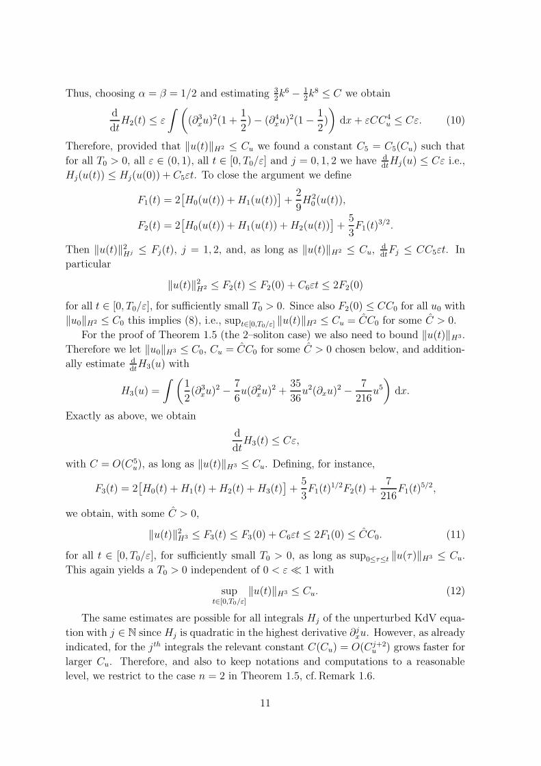
Figure 1: The inclined-film problem: A fluid of height y = h(x, t) = h0 + u(x, t) runs down a

plate with inclination angle θ subject to constant gravitational force g. In appropriate ranges

of parameters (1) is the amplitude equation for this problem, where t, x, u are rescalings of

t, x and u.

For ε = 0 equation (1) is the well known KdV equation for which there exist

2n-dimensional families Mn of n-soliton solutions; see, e.g, [AS81]. For n = 1 the

two-dimensional family M1 is explicitly given by

M1 = {u(x, t) = uc(x− ct+ φ) : φ ∈ R, c > 0}, uc(y) = 3c sech2(√cy/2).

The amplitude parameter c also determines the speed, and φ is called the phase. For

small ε > 0 there is an amplitude/speed selection principle [Oga94]: there exists a

unique velocity cε = 7/5 +O(ε) and a one-dimensional family of solitary waves for (1)

of the form

Mε = {u(x, t) = uε(x− cεt+ φ) : φ ∈ R}with ‖uε−ucε‖H1 ≤ C0ε. In particular ‖uε‖L∞ = O(1) for ε→ 0, and |uε(y)| ≤ Ce−β0|y|

with constants C and β0 > 0 both O(1) for ε→ 0.

For all ε > 0 the pulse uε is unstable since the linearization around uε gives the

same essential spectrum as the medium, the unstable trivial solution u = 0. However,

a remarkable phenomenon occurs: in numerical simulations, the pulse uε is stable on

long (but finite) time intervals. More generally speaking, the dynamics is dominated

by KdV pulses over long times. On the other hand, for t → ∞ the solution generally

converges to a traveling pulse train consisting of (boosts of) the individually unstable

pulses uε. See fig. 2 for an example. Such dynamics of surface waves are typical of

observations in the inclined film problem [CD02], both experimentally and in numerical

simulations of the free boundary Navier-Stokes problem describing this system.

The local-in-time stability of uε based on spectral information has been analyzed

in [CDK96, OS97, CDK98, PSU04]; additionally, see [CD02] and the references therein

for the structure of families of traveling wave solutions to (1) which is a first step in the

analysis of the large time behaviour of (1). To add to the understanding of the long- but

2

(a) (b)

-400

x=400

100

t=20004

-400

x=40400

500

t=600-13

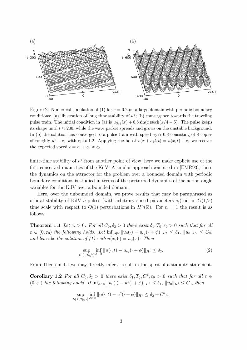
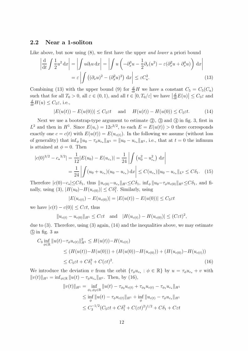
Figure 2: Numerical simulation of (1) for ε = 0.2 on a large domain with periodic boundary

conditions: (a) illustration of long time stability of uε; (b) convergence towards the traveling

pulse train. The initial condition in (a) is u3/2(x) + 0.8 sin(x)sech(x/4 − 5). The pulse keeps

its shape until t ≈ 200, while the wave packet spreads and grows on the unstable background.

In (b) the solution has converged to a pulse train with speed c0 ≈ 0.3 consisting of 8 copies

of roughly uε − c1 with c1 ≈ 1.2. Applying the boost v(x + c1t, t) = u(x, t) + c1 we recover

the expected speed c = c1 + c0 ≈ cε.

finite-time stability of uε from another point of view, here we make explicit use of the

first conserved quantities of the KdV. A similar approach was used in [EMR93]; there

the dynamics on the attractor for the problem over a bounded domain with periodic

boundary conditions is studied in terms of the perturbed dynamics of the action angle

variables for the KdV over a bounded domain.

Here, over the unbounded domain, we prove results that may be paraphrased as

orbital stability of KdV n-pulses (with arbitrary speed parameters cj) on an O(1/ε)

time scale with respect to O(1) perturbations in Hn(R). For n = 1 the result is as

follows.

Theorem 1.1 Let c? > 0. For all C0, δ2 > 0 there exist δ1, T0, ε0 > 0 such that for all

ε ∈ (0, ε0) the following holds. Let infφ∈R ‖u0(·) − uc?(· + φ)‖H1 ≤ δ1, ‖u0‖H2 ≤ C0,

and let u be the solution of (1) with u(x, 0) = u0(x). Then

supt∈[0,T0/ε]

infφ∈R

‖u(·, t) − uc?(· + φ)‖H1 ≤ δ2. (2)

From Theorem 1.1 we may directly infer a result in the spirit of a stability statement.

Corollary 1.2 For all C0, δ2 > 0 there exist δ1, T0, C?, ε0 > 0 such that for all ε ∈

(0, ε0) the following holds. If infφ∈R ‖u0(·) − uε(· + φ)‖H1 ≤ δ1, ‖u0‖H2 ≤ C0, then

supt∈[0,T0/ε]

infφ∈R

‖u(·, t) − uε(· + φ)‖H1 ≤ δ2 + C?ε.

3

The proof of Theorem 1.1 is based on the orbital stability proof for KdV 1-solitons

given in [Ben72, Bo75], i.e., the orbital stability of uc in the case ε = 0. There it is

shown that the Hamiltonian

H(u) =

∫(

1

2(∂xu)

2 − 1

6u3

)

dx

of the KdV equation has a line of minima along the orbit {τφuc : φ ∈ R}, τφuc(·) =

uc(· + φ), under the constraint

E(u) =

∫

1

2u2 dx = const.

In fact, this constraint yields the first part in the inequality

C3 infφ∈R

‖u− τφuc‖2H1 ≤ H(u) −H(uc) ≤ C4‖u− uc‖2

H1 , (3)

with C3, C4 > 0, which implies the orbital stability of a pulse uc in the KdV-equation.

Here we adapt this proof to (1) with ε > 0 by proving a priori estimates

H(u(t)) −H(u0) + |E(u(t)) − E(u0)| ≤ Cεt. (4)

On the other hand, the mass

M(u) =

∫

u(x) dx

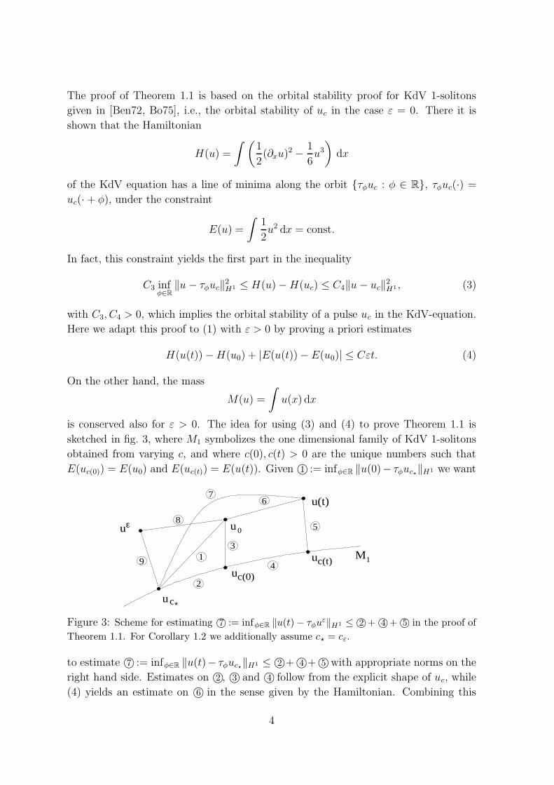
is conserved also for ε > 0. The idea for using (3) and (4) to prove Theorem 1.1 is

sketched in fig. 3, where M1 symbolizes the one dimensional family of KdV 1-solitons

obtained from varying c, and where c(0), c(t) > 0 are the unique numbers such that

E(uc(0)) = E(u0) and E(uc(t)) = E(u(t)). Given ©1 := infφ∈R ‖u(0)− τφuc?‖H1 we want

uc(0)

uε

uc

uc(t)

u0

2

u(t)

M1

3

4

5

6

1

8

7

9

∗

Figure 3: Scheme for estimating ©7 := infφ∈R ‖u(t) − τφuε‖H1 ≤ ©2 + ©4 + ©5 in the proof of

Theorem 1.1. For Corollary 1.2 we additionally assume c? = cε.

to estimate ©7 := infφ∈R ‖u(t)− τφuc?‖H1 ≤ ©2 +©4 +©5 with appropriate norms on the

right hand side. Estimates on ©2 , ©3 and ©4 follow from the explicit shape of uc, while

(4) yields an estimate on ©6 in the sense given by the Hamiltonian. Combining this

4

with (3) we then obtain an estimate on ©5 ≤ ©6 + ©3 + ©4 in the H1 sense. If c? = cε,

then the estimate in Corollary 1.2 follows from ©9 = O(ε) in H1. In order to prove

(4) we additionally need a priori estimates on the next integral H2 of the unperturbed

KdV equation.

Remark 1.3 Theorem 1.1 improves the local in time and space stability result from

[PSU04, Theorem 5.1] in two directions: Theorem 1.1 is global and not only local

in space; i.e., no weight in space is needed, and the allowed magnitude of the initial

perturbations in Theorem 1.1 is O(1) and not O(ε) as in [PSU04]. c

Remark 1.4 Besides the local-in-time stability stated in Theorem 1.1, also the local-

in-space attractivity of the pulses proved in [CDK96, PSU04] helps to explain why the

dynamics of (1) is dominated by essentially unstable pulses. Due to the fact that the

local-in-space attractive two-dimensional structure found in [PSU04] is not invariant

under the flow of (1) and does not lie in the phase space H1(R), the method of [PW94]

cannot be applied directly. Therefore, the attractivity result [PSU04, Theorem 5.1] is

not improved substantially using the a priori estimates from the proof of Theorem 1.1.

However, the coefficients δv(0) and δw(0) from [PSU04, Theorem 5.1], which describe

the magnitude of the initial perturbations in an unweighted and a weighted norm, can

now be chosen up to order O(1) in H1(R) instead of O(ε), and O(ε2) in Hn(R) for

general n, respectively. c

The orbital H1-stability result for KdV 1-solitons has been generalized to Hn-stability

for n-solitons in [MS93]. (Recently, higher-order Hm-stability of 1-solitons was studied

in [BLN04].) For fixed n ≥ 2, KdV n-solitons are given by a 2n-parameter family of pro-

files u(n)(y; c1, . . . , cn, φ1, . . . , φn). For instance, for n = 2 we have u(2) = 12∂2y log(τ (2))

where

τ (2) =1 + exp(√c1(y + φ1)) + exp(

√c2(y + φ2))

+

(√c1 −

√c2√

c1 +√c2

)2

exp(√c1(y + φ1) +

√c2(y + φ2)).

(5)

The time-dependent 2-soliton solution of KdV then is

u~c(x, t; ~φ) = u(2)(x; c1, c2, φ1 − c1t, φ2 − c2t).

Below we shall often omit the phases ~φ when they are not important, for instance in

the evaluation of conserved quantities like E and H.

There is an important difference for the notion of stability of the families of n-

solitons for n = 1 and n ≥ 2. For n = 1 and given c, the time orbit of a 1-soliton, or

equivalently the orbit of its spatial translates, traverses the full family M1(c), while for

n ≥ 2 and given ~c, the time orbit and the spatial translates only traverse (different)

one-dimensional submanifolds of Mn(~c). Consequently, for n ≥ 2 there is a somewhat

5

different notion of orbital stability of KdV n-solitons, namely that solutions stay close

to n-soliton profiles with given ~c but varying ~φ. For (1) with ε > 0 and n = 2 (see

Remark 1.6) we then have:

Theorem 1.5 Let ~c? ∈ R2+. For all C0, δ2 > 0 there exist δ1, T0, ε0 > 0 such that for

all ε ∈ (0, ε0) the following holds. Let ‖u0(·) − u(2)(·,~c?, ~φ)‖H2 ≤ δ1 for some ~φ ∈ R2,

‖u0‖H3 ≤ C0, and let u be the solution of (1) with u(x, 0) = u0(x). Then

supt∈[0,T0/ε]

inf~φ∈R2

‖u(·, t) − u(2)(·,~c?, ~φ)‖H2 ≤ δ2. (6)

The proof of Theorem 1.5 uses the same idea as sketched for Theorem 1.1 in fig. 3,

namely the fact [MS93] that 2-solitons are minimizers of the next integral

H2(u) =

∫(

1

2(∂2xu)

2 − 5

6u(∂xu)

2 +5

72u4

)

dx (7)

of the KdV equation under the constraints E(u), H(u) = const.

Remark 1.6 The generalization of Theorem 1.5 to n ≥ 2 is true for all n, with

constants independent of ε, but these constants depend on n. For instance, T0 typically

decreases with increasing n. Therefore, for large n the result will be more of theoretical

interest, while for smaller n the O(1/ε) time scale n-soliton dynamics can be well traced

also in numerical simulation of (1), i.e., T0 can be chosen rather large in (2) and (6).

Moreover, for large n the computations become lengthy. Therefore, here we restrict to

n = 2; further explications for the general case are given in sec. 2.3. c

Theorem 1.5 itself does not imply that the solitons really interact, cf. the discussion

in [MS93] for the unperturbed KdV equation. However, a soliton interaction that

happens on an O(1) time scale in the unperturbed KdV equation also occurs in the

KS–perturbed KdV equation due to the following approximation theorem. Numerical

illustrations of local-in-time 2-soliton dynamics in (1) are given in figures 4 and 5.

Theorem 1.7 Fix an integer s ≥ 2. For all C1, T0 > 0 there exist ε0, C2 > 0 such

that for all ε ∈ (0, ε0) the following holds. For all solutions v ∈ C([0, T0], Hs+4) of

the KdV–equation ∂tv = −∂3xv −

1

2∂x(v

2) satisfying supt∈[0,T0]

‖v(t)‖Hs+4 ≤ C1 there is a

solution u ∈ C([0, T0], Hs) of (1) with

supt∈[0,T0]

‖u(t) − v(t)‖Hs ≤ C2ε .

Proof. A solution u of (1) is a sum of the KdV solution v and an error function εR,

i.e., u = v + εR. We find

∂tR = − ∂3xR− ∂x(vR) − ε

2∂x(R

2) − ε(∂2x + ∂4

x)R− (∂2x + ∂4

x)v,

6

(a) (b)

-40

0

x=40

0

30

60

90

t=120

04

-40

0

x=40

150

t=250

04

(c) (d) E, H (dashed) and H2 (dotted),

normalized by E(0), H(0) and H2(0)

-40

0

x=40

650

750

t=850

04

0

1

2

3

4

0 200 400 600 800 1000

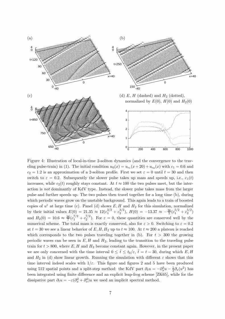
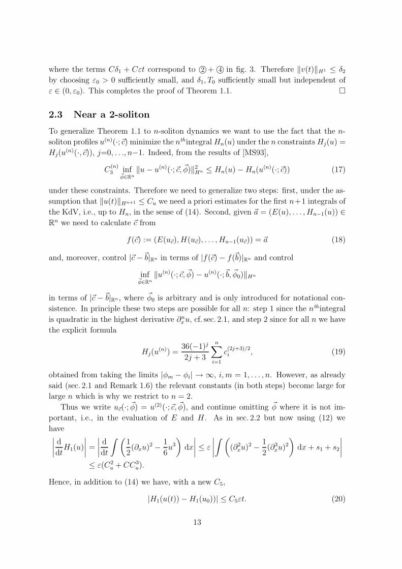
Figure 4: Illustration of local-in-time 2-soliton dynamics (and the convergence to the trav-

eling pulse-train) in (1). The initial condition u0(x) = uc1(x+20)+uc2 (x) with c1 = 0.6 and

c2 = 1.2 is an approximation of a 2-soliton profile. First we set ε = 0 until t = 30 and then

switch to ε = 0.2. Subsequently the slower pulse takes up mass and speeds up, i.e., c1(t)

increases, while c2(t) roughly stays constant. At t ≈ 100 the two pulses meet, but the inter-

action is not dominantly of KdV type. Instead, the slower pulse takes mass from the larger

pulse and further speeds up. The two pulses then travel together for a long time (b), during

which periodic waves grow on the unstable background. This again leads to a train of boosted

copies of uε at large time (c). Panel (d) shows E,H and H2 for this simulation, normalized

by their initial values E(0) = 21.35 ≈ 12(c3/21 + c

3/22 ), H(0) = −13.37 ≈ − 36

5 (c5/21 + c

5/22 )

and H2(0) = 10.6 ≈ 367 (c

7/21 + c

7/22 ). For ε = 0, these quantities are conserved well by the

numerical scheme. The total mass is exactly conserved, also for ε > 0. Switching to ε = 0.2

at t = 30 we see a linear behavior of E,H,H2 up to t ≈ 100. At t ≈ 200 a plateau is reached

which corresponds to the two pulses traveling together in (b). For t > 300 the growing

periodic waves can be seen in E,H and H2, leading to the transition to the traveling pulse

train for t > 800, where E,H and H2 become constant again. However, in the present paper

we are only concerned with the time interval 0 ≤ t ≤ t0/ε, t = t − 30, during which E,H

and H2 in (d) show linear growth. Running the simulation with different ε shows that this

time interval indeed scales with 1/ε. This figure and figures 2 and 5 have been produced

using 512 spatial points and a split-step method: the KdV part ∂tu = −∂3xu − 1

2∂x(u2) has

been integrated using finite difference and an explicit leap-frog scheme [ZK65], while for the

dissipative part ∂tu = −ε(∂2x + ∂4

x)u we used an implicit spectral method.

7

which via partial integration implies

1

2∂t

∫

(∂sxR)2 dx = −∫

(∂sxR)∂s+1x (vR) dx− ε

2

∫

(∂sxR)∂s+1x (R2) dx

+

∫

ε((∂s+1x R)2 − (∂s+2

x R)2) dx−∫

(∂sxR)∂sx(∂2x + ∂4

x)v dx .

Next∫

(∂sxR)∂s+1x (vR) dx = −1

2

∫

(∂sxR)2(∂xv) dx+ O(‖v‖Hs+1‖R‖2Hs) ,

∫

(∂sxR)∂s+1x (R2) dx = −

∫

(∂sxR)2(∂xR) dx+ O(‖R‖3Hs) ,

∫

(∂s+1x R)2 − (∂s+2

x R)2 dx ≤ 1

4‖∂sxR‖2

L2 .

Thus the Cauchy–Schwarz inequality yields

∂t(‖R‖2Hs) ≤ C(‖R‖2

Hs + ε‖R‖3Hs + C2

1)

with a constant C independent of 0 < ε� 1. For all t ≥ 0, as long as ε‖R(t)‖3Hs ≤ 1,

Gronwall’s inequality implies

supt∈[0,T0]

‖R(t)‖Hs ≤ C(1 + C21)T0 e

CT0 =: C .

We are done by choosing ε > 0 so small that εC3 ≤ 1. �

Remark 1.8 The phenomena explained in this paper occurs at a time of order O(1/ε)

which is beyond the O(1) time interval of validity of (1) for the inclined-film problem.

Except for special limits, (1) only serves as a phenomenological model for going beyond

the pure KdV dynamics valid on the O(1)-time interval. c

2 The proofs

2.1 A priori estimates

Let Cu = CC0 with C > 0 chosen below. First we prove that there is a T0 > 0

independent of 0 < ε� 1 such that

supt∈[0,T0/ε]

‖u(t)‖H2 ≤ Cu. (8)

In order to do so we prove upper bounds for the time derivatives of the first three

integrals of the unperturbed KdV equation, using the convention that H0(u)=E(u).

The estimates are obtained in such a way that for the j-th integral we only use estimates

8

(a) (b)

-400

x=40

t=0

t=100

2

4

-400

x=40

t=0

t=100

2

4

(c) (d)

-400

x=40

t=0

t=100

2

4

-400

x=40

t=0

t=100

2

4

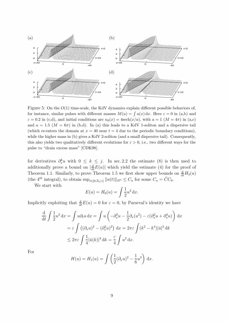
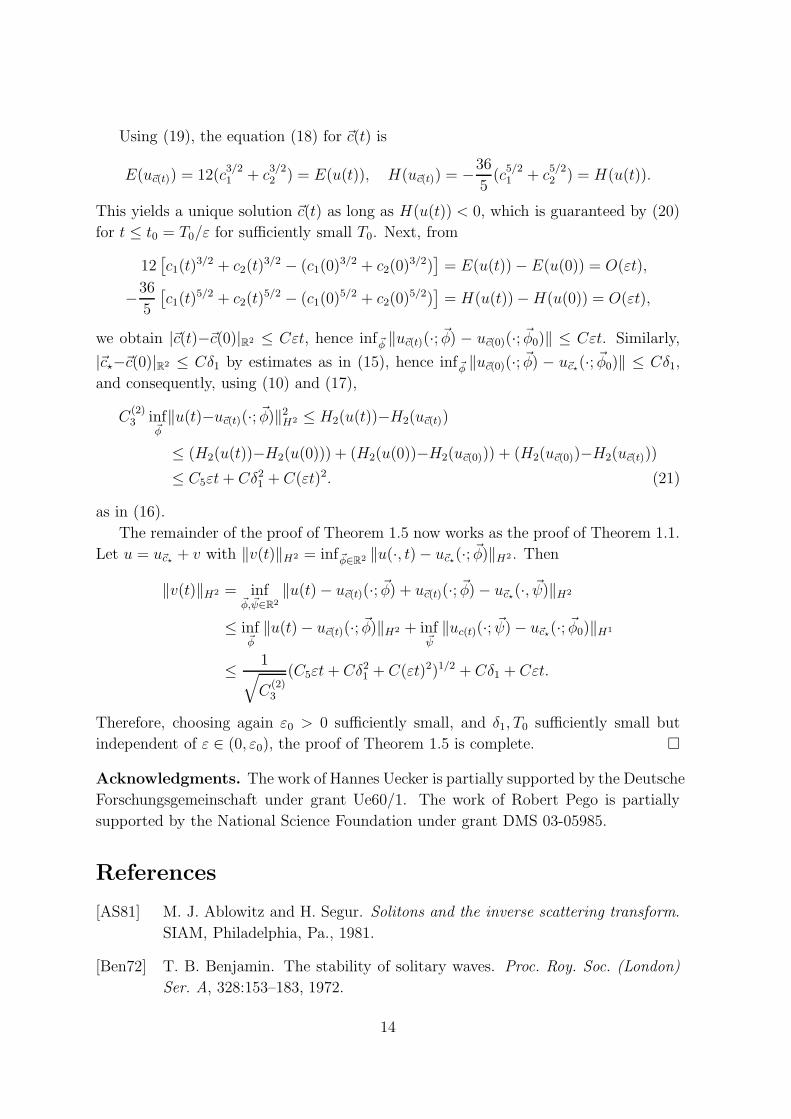
Figure 5: On the O(1) time-scale, the KdV dynamics explain different possible behaviors of,

for instance, similar pulses with different masses M(u) =∫

u(x) dx. Here ε = 0 in (a,b) and

ε = 0.2 in (c,d), and initial conditions are u0(x) = 4sech(x/a), with a = 1 (M = 4π) in (a,c)

and a = 1.5 (M = 6π) in (b,d). In (a) this leads to a KdV 1-soliton and a dispersive tail

(which re-enters the domain at x = 40 near t = 4 due to the periodic boundary conditions),

while the higher mass in (b) gives a KdV 2-soliton (and a small dispersive tail). Consequently,

this also yields two qualitatively different evolutions for ε > 0, i.e., two different ways for the

pulse to “drain excess mass” [CDK98].

for derivatives ∂kxu with 0 ≤ k ≤ j. In sec. 2.2 the estimate (8) is then used to

additionally prove a bound on | ddtE(u)| which yield the estimate (4) for the proof of

Theorem 1.1. Similarly, to prove Theorem 1.5 we first show upper bounds on ddtH3(u)

(the 4th integral), to obtain supt∈[0,T0/ε] ‖u(t)‖H3 ≤ Cu for some Cu = CC0.

We start with

E(u) = H0(u) =

∫

1

2u2 dx.

Implicitly exploiting that ddtE(u) = 0 for ε = 0, by Parseval’s identity we have

d

dt

∫

1

2u2 dx =

∫

u∂tu dx =

∫

u

(

−∂3xu−

1

2∂x(u

2) − ε(∂2xu+ ∂4

xu)

)

dx

= ε

∫

(

(∂xu)2 − (∂2

xu)2)

dx = 2πε

∫

(k2 − k4)|u|2 dk

≤ 2πε

∫

1

4|u(k)|2 dk =

ε

4

∫

u2 dx.

For

H(u) = H1(u) =

∫(

1

2(∂xu)

2 − 1

6u3

)

dx.

9

we find, using ddtH(u) = 0 for ε = 0,

d

dt

∫(

1

2(∂xu)

2 − 1

6u3

)

dx =

∫(

(∂xu)(∂x∂tu) −1

2u2∂tu

)

dx

=

∫(

(∂xu)∂x(

−ε(∂2x+∂

4x)u

)

− 1

2u2

(

−ε(∂2x+∂

4x)u

)

)

dx = ε(s0 + s1 + s2)

with

s0 =

∫

(∂2xu)

2 − (∂3xu)

2 dx, s1 =

∫

1

2u2(∂2

xu) dx, s2 =

∫

1

2u2(∂4

xu) dx.

Presuming ‖u(t)‖H1 ≤ Cu for the t under consideration shows |s1| = |−∫

u(∂xu)2 dx| ≤

C3u. Moreover, using |ab| ≤ 1

2(ηa2 + η−1b2), η > 0, we obtain

|s2| =

∣

∣

∣

∣

−∫

u(∂xu)(∂3xu) dx

∣

∣

∣

∣

≤ Cu

∣

∣

∣

∣

∫

(

η−1(∂xu)2 + η(∂3

xu)2)

dx

∣

∣

∣

∣

≤ Cδ + δ‖∂3xu‖2

L2

with a constant Cδ → ∞ for δ → 0. Choosing δ = 1/2 and estimating k4 − k6/2 ≤ C

with a constant C independent of k as in the estimate for ddtE, we obtain

d

dt

∫(

1

2(∂xu)

2 − 1

6u3

)

dx ≤ ε

∫(

(∂2xu)

2 − 1

2(∂3xu)

2

)

dx+ ε(C1/2 + C3u)

= 2πε

∫

(k4 − 1

2k6)|u(k)|2 dk + ε(C1/2 + C3

u) ≤ ε(C‖u‖2L2 + C1/2 + C3

u)

≤ Cε (9)

for a C > 0.

Next we consider

H2(u) =

∫(

1

2(∂2xu)

2 − 5

6u(∂xu)

2 +5

72u4

)

dx

and t such that ‖u(t)‖H2 ≤ Cu. We have, using ddtH2 = 0 for ε = 0,

d

dtH2(t) =

∫

∂tu

(

∂4xu−

5

6(∂xu)

2 +5

6∂2x(u

2) +5

18u3

)

dx = ε(s0 + s1 + s2 + s3)

with s0 =∫

(∂3xu)

2 − (∂4xu)

2 dx and

|s1| =

∣

∣

∣

∣

∫

(∂2xu)

(

5

18u3 +

5

18∂2x(u

3)

)

dx

∣

∣

∣

∣

≤ 5C4u,

|s2| =5

6

∣

∣

∣

∣

∫

(∂2xu+ ∂4

xu)∂2x(u

2) dx

∣

∣

∣

∣

≤ 2C3u +

5

12

∫

(

η(∂4xu)

2 + η−1(∂2x(u

2))2)

dx ≤ α‖∂4xu‖2

L2 + Cα,

|s3| =5

6

∣

∣

∣

∣

∫

(

(∂xu)2∂2xu− (∂x(∂xu)

2)(∂3xu)

)

dx

∣

∣

∣

∣

≤ C3u +

5

12

∫

(

η(∂3xu)

2 + η−1(∂x(∂xu)2)2

)

dx ≤ β‖∂3xu‖2

L2 + Cβ.

10

Thus, choosing α = β = 1/2 and estimating 32k6 − 1

2k8 ≤ C we obtain

d

dtH2(t) ≤ ε

∫(

(∂3xu)

2(1 +1

2) − (∂4

xu)2(1 − 1

2)

)

dx + εCC4u ≤ Cε. (10)

Therefore, provided that ‖u(t)‖H2 ≤ Cu we found a constant C5 = C5(Cu) such that

for all T0 > 0, all ε ∈ (0, 1), all t ∈ [0, T0/ε] and j = 0, 1, 2 we have ddtHj(u) ≤ Cε i.e.,

Hj(u(t)) ≤ Hj(u(0)) + C5εt. To close the argument we define

F1(t) = 2[

H0(u(t)) +H1(u(t))]

+2

9H2

0 (u(t)),

F2(t) = 2[

H0(u(t)) +H1(u(t)) +H2(u(t))]

+5

3F1(t)

3/2.

Then ‖u(t)‖2Hj ≤ Fj(t), j = 1, 2, and, as long as ‖u(t)‖H2 ≤ Cu,

ddtFj ≤ CC5εt. In

particular

‖u(t)‖2H2 ≤ F2(t) ≤ F2(0) + C6εt ≤ 2F2(0)

for all t ∈ [0, T0/ε], for sufficiently small T0 > 0. Since also F2(0) ≤ CC0 for all u0 with

‖u0‖H2 ≤ C0 this implies (8), i.e., supt∈[0,T0/ε] ‖u(t)‖H2 ≤ Cu = CC0 for some C > 0.

For the proof of Theorem 1.5 (the 2–soliton case) we also need to bound ‖u(t)‖H3.

Therefore we let ‖u0‖H3 ≤ C0, Cu = CC0 for some C > 0 chosen below, and addition-

ally estimate ddtH3(u) with

H3(u) =

∫(

1

2(∂3xu)

2 − 7

6u(∂2

xu)2 +

35

36u2(∂xu)

2 − 7

216u5

)

dx.

Exactly as above, we obtain

d

dtH3(t) ≤ Cε,

with C = O(C5u), as long as ‖u(t)‖H3 ≤ Cu. Defining, for instance,

F3(t) = 2[

H0(t) +H1(t) +H2(t) +H3(t)]

+5

3F1(t)

1/2F2(t) +7

216F1(t)

5/2,

we obtain, with some C > 0,

‖u(t)‖2H3 ≤ F3(t) ≤ F3(0) + C6εt ≤ 2F1(0) ≤ CC0. (11)

for all t ∈ [0, T0/ε], for sufficiently small T0 > 0, as long as sup0≤τ≤t ‖u(τ)‖H3 ≤ Cu.

This again yields a T0 > 0 independent of 0 < ε� 1 with

supt∈[0,T0/ε]

‖u(t)‖H3 ≤ Cu. (12)

The same estimates are possible for all integrals Hj of the unperturbed KdV equa-

tion with j ∈ N since Hj is quadratic in the highest derivative ∂jxu. However, as already

indicated, for the jth integrals the relevant constant C(Cu) = O(Cj+2u ) grows faster for

larger Cu. Therefore, and also to keep notations and computations to a reasonable

level, we restrict to the case n = 2 in Theorem 1.5, cf. Remark 1.6.

11

2.2 Near a 1-soliton

Like above, but now using (8), we first have the upper and lower a priori bound∣

∣

∣

∣

d

dt

∫

1

2u2 dx

∣

∣

∣

∣

=

∣

∣

∣

∣

∫

u∂tu dx

∣

∣

∣

∣

=

∣

∣

∣

∣

∫

u

(

−∂3xu−

1

2∂x(u

2) − ε(∂2xu+ ∂4

xu)

)

dx

∣

∣

∣

∣

= ε

∣

∣

∣

∣

∫

(

(∂xu)2 − (∂2

xu)2)

dx

∣

∣

∣

∣

≤ εC2u. (13)

Combining (13) with the upper bound (9) for ddtH we have a constant C5 = C5(Cu)

such that for all T0 > 0, all ε ∈ (0, 1), and all t ∈ [0, T0/ε] we have∣

∣

ddtE(u)

∣

∣ ≤ C5ε andddtH(u) ≤ C5ε, i.e.,

|E(u(t)) − E(u(0))| ≤ C5εt and H(u(t)) −H(u(0)) ≤ C5εt. (14)

Next we use a bootstrap-type argument to estimate ©2 , ©3 and ©4 in fig. 3, first in

L2 and then in H1. Since E(uc) = 12c3/2, to each E = E(u(t)) > 0 there corresponds

exactly one c = c(t) with E(u(t)) = E(uc(t)). In the following we assume (without loss

of generality) that infφ ‖u0 − τφuc?‖H1 = ‖u0 − uc?‖H1 , i.e., that at t = 0 the infimum

is attained at φ = 0. Then

|c(0)3/2 − c?3/2| =

1

12|E(u0) − E(uc?)| =

1

24

∣

∣

∣

∣

∫

(

u20 − u2

c?

)

dx

∣

∣

∣

∣

=1

24

∣

∣

∣

∣

∫

(u0 + uc?)(u0 − uc?) dx

∣

∣

∣

∣

≤ C(uc?)‖u0 − uc?‖L2 ≤ Cδ1. (15)

Therefore |c(0)−c?|≤Cδ1, thus ‖uc(0)−uc?‖H1≤Cδ1, infφ ‖u0−τφuc(0)‖H1≤Cδ1, and fi-

nally, using (3), |H(u0)−H(uc(0))| ≤ Cδ21 . Similarly, using

|E(uc(t)) − E(uc(0))| = |E(u(t)) − E(u(0))| ≤ C5εt

we have |c(t) − c(0)| ≤ Cεt, thus

‖uc(t) − uc(0)‖H1 ≤ Cεt and |H(uc(t)) −H(uc(0))| ≤ (Cεt)2,

due to (3). Therefore, using (3) again, (14) and the inequalities above, we may estimate

©5 in fig. 3 as

C3 infφ∈R

‖u(t)−τφuc(t)‖2H1 ≤ H(u(t))−H(uc(t))

≤ (H(u(t))−H(u(0))) + (H(u(0))−H(uc(0))) + (H(uc(0))−H(uc(t)))

≤ C5εt+ Cδ21 + C(εt)2. (16)

We introduce the deviation v from the orbit {τφuc? : φ ∈ R} by u = τφuc? + v with

‖v(t)‖H1 = infφ∈R ‖u(t) − τφuc?‖H1 . Then, by (16),

‖v(t)‖H1 = infφ1,φ2∈R

‖u(t) − τφ2uc(t) + τφ2

uc(t) − τφ1uc?‖H1

≤ infφ‖u(t) − τφuc(t)‖H1 + inf

φ‖uc(t) − τφuc?‖H1

≤ C−1/23 (C5εt+ Cδ2

1 + C(εt)2)1/2 + Cδ1 + Cεt

12

where the terms Cδ1 + Cεt correspond to ©2 + ©4 in fig. 3. Therefore ‖v(t)‖H1 ≤ δ2by choosing ε0 > 0 sufficiently small, and δ1, T0 sufficiently small but independent of

ε ∈ (0, ε0). This completes the proof of Theorem 1.1. �

2.3 Near a 2-soliton

To generalize Theorem 1.1 to n-soliton dynamics we want to use the fact that the n-

soliton profiles u(n)(·;~c) minimize the nth integralHn(u) under the n constraints Hj(u) =

Hj(u(n)(·,~c)), j=0, . . ., n−1. Indeed, from the results of [MS93],

C(n)3 inf

~φ∈Rn

‖u− u(n)(·;~c, ~φ)‖2Hn ≤ Hn(u) −Hn(u

(n)(·;~c)) (17)

under these constraints. Therefore we need to generalize two steps: first, under the as-

sumption that ‖u(t)‖Hn+1 ≤ Cu we need a priori estimates for the first n+1 integrals of

the KdV, i.e., up to Hn, in the sense of (14). Second, given ~a = (E(u), . . . , Hn−1(u)) ∈Rn we need to calculate ~c from

f(~c) := (E(u~c), H(u~c), . . . , Hn−1(u~c)) = ~a (18)

and, moreover, control |~c−~b|Rn in terms of |f(~c) − f(~b)|Rn and control

inf~φ∈Rn

‖u(n)(·;~c, ~φ) − u(n)(·;~b, ~φ0)‖Hn

in terms of |~c−~b|Rn, where ~φ0 is arbitrary and is only introduced for notational con-

sistence. In principle these two steps are possible for all n: step 1 since the nth integral

is quadratic in the highest derivative ∂nxu, cf. sec. 2.1, and step 2 since for all n we have

the explicit formula

Hj(u(n)) =

36(−1)j

2j + 3

n∑

i=1

c(2j+3)/2i , (19)

obtained from taking the limits |φm − φi| → ∞, i,m = 1, . . . , n. However, as already

said (sec. 2.1 and Remark 1.6) the relevant constants (in both steps) become large for

large n which is why we restrict to n = 2.

Thus we write u~c(·; ~φ) = u(2)(·;~c, ~φ), and continue omitting ~φ where it is not im-

portant, i.e., in the evaluation of E and H. As in sec. 2.2 but now using (12) we

have∣

∣

∣

∣

d

dtH1(u)

∣

∣

∣

∣

=

∣

∣

∣

∣

d

dt

∫(

1

2(∂xu)

2 − 1

6u3

)

dx

∣

∣

∣

∣

≤ ε

∣

∣

∣

∣

∫(

(∂2xu)

2 − 1

2(∂3xu)

2

)

dx + s1 + s2

∣

∣

∣

∣

≤ ε(C2u + CC3

u).

Hence, in addition to (14) we have, with a new C5,

|H1(u(t)) −H1(u0))| ≤ C5εt. (20)

13

Using (19), the equation (18) for ~c(t) is

E(u~c(t)) = 12(c3/21 + c

3/22 ) = E(u(t)), H(u~c(t)) = −36

5(c

5/21 + c

5/22 ) = H(u(t)).

This yields a unique solution ~c(t) as long as H(u(t)) < 0, which is guaranteed by (20)

for t ≤ t0 = T0/ε for sufficiently small T0. Next, from

12[

c1(t)3/2 + c2(t)

3/2 − (c1(0)3/2 + c2(0)3/2)]

= E(u(t)) − E(u(0)) = O(εt),

−36

5

[

c1(t)5/2 + c2(t)

5/2 − (c1(0)5/2 + c2(0)5/2)]

= H(u(t)) −H(u(0)) = O(εt),

we obtain |~c(t)−~c(0)|R2 ≤ Cεt, hence inf ~φ ‖u~c(t)(·; ~φ) − u~c(0)(·; ~φ0)‖ ≤ Cεt. Similarly,

|~c?−~c(0)|R2 ≤ Cδ1 by estimates as in (15), hence inf ~φ ‖u~c(0)(·; ~φ) − u~c?(·; ~φ0)‖ ≤ Cδ1,

and consequently, using (10) and (17),

C(2)3 inf

~φ‖u(t)−u~c(t)(·; ~φ)‖2

H2 ≤ H2(u(t))−H2(u~c(t))

≤ (H2(u(t))−H2(u(0))) + (H2(u(0))−H2(u~c(0))) + (H2(u~c(0))−H2(u~c(t)))

≤ C5εt+ Cδ21 + C(εt)2. (21)

as in (16).

The remainder of the proof of Theorem 1.5 now works as the proof of Theorem 1.1.

Let u = u~c? + v with ‖v(t)‖H2 = inf ~φ∈R2 ‖u(·, t) − u~c?(·; ~φ)‖H2 . Then

‖v(t)‖H2 = inf~φ,~ψ∈R2

‖u(t) − u~c(t)(·; ~φ) + u~c(t)(·; ~φ) − u~c?(·, ~ψ)‖H2

≤ inf~φ‖u(t) − u~c(t)(·; ~φ)‖H2 + inf

~ψ‖uc(t)(·; ~ψ) − u~c?(·; ~φ0)‖H1

≤ 1√

C(2)3

(C5εt+ Cδ21 + C(εt)2)1/2 + Cδ1 + Cεt.

Therefore, choosing again ε0 > 0 sufficiently small, and δ1, T0 sufficiently small but

independent of ε ∈ (0, ε0), the proof of Theorem 1.5 is complete. �

Acknowledgments. The work of Hannes Uecker is partially supported by the Deutsche

Forschungsgemeinschaft under grant Ue60/1. The work of Robert Pego is partially

supported by the National Science Foundation under grant DMS 03-05985.

References

[AS81] M. J. Ablowitz and H. Segur. Solitons and the inverse scattering transform.

SIAM, Philadelphia, Pa., 1981.

[Ben72] T. B. Benjamin. The stability of solitary waves. Proc. Roy. Soc. (London)

Ser. A, 328:153–183, 1972.

14

[Bo75] J. L. Bona. On the stability of solitary waves. Proc. Roy. Soc. (London) Ser.

A, 344:363–374, 1975.

[BLN04] J. L. Bona, Y. Liu and N. V. Nguyen. Stability of solitary waves in higher-

order Sobolev spaces. Comm. Math. Sci., 2(1):35–52, 2004.

[CD96] H.-C. Chang and E. A. Demekhin. Solitary wave formation and dynamics

on falling films. Adv. Appl. Mech., 32:1–58, 1996.

[CD02] H.-C. Chang and E.A. Demekhin. Complex Wave Dynamics on Thin Films.

Elsevier, Amsterdam, 2002.

[CDK96] H.-C. Chang, E.A. Demekhin, and D.I. Kopelevich. Local stability theory of

solitary pulses in an active medium. Physica D, 97:353–375, 1996.

[CDK98] H.-C. Chang, E.A. Demekhin, and E. Kalaidin. Generation and suppression

of radiation by solitary pulses. SIAM J. Appl. Math., 58(4):1246–1277, 1998.

[EMR93] N. M. Ercolani, D. W. McLaughlin, and H. Roitner. Attractors and transients

for a perturbed periodic KdV equation: a nonlinear spectral analysis. J.

Nonlinear Sci., 3(4):477–539, 1993.

[Kat81] T. Kato. The Cauchy problem for the Korteweg-de Vries equation. In Non-

linear partial differential equations and their applications. College de France

Seminar, Vol. I (Paris, 1978/1979), volume 53 of Res. Notes in Math., pages

293–307. Pitman, 1981.

[KPV91] C. E. Kenig, G. Ponce, and L. Vega. Well-posedness of the initial value

problem for the Korteweg-de Vries equation. J. Amer. Math. Soc., 4(2):323–

347, 1991.

[MS93] J. H. Maddocks and R. L. Sachs. On the stability of KdV multi-solitons.

Comm. Pure Appl. Math., 46(6):867–901, 1993.

[Oga94] T. Ogawa. Travelling wave solutions to a perturbed Korteweg–de Vries equa-

tion. Hiroshima Math. J., 24:401–422, 1994.

[OS97] T. Ogawa and H. Susuki. On the spectra of pulses in a nearly integrable

system. SIAM J. Appl. Math., 57(2):485–500, 1997.

[PSU04] R.L. Pego, G. Schneider, and H. Uecker. Local in time and space nonlinear

stability of pulses in an unstable medium. To appear in Proceedings ICMP,

Lisboa, 2003, 2004.

[PW94] R.L. Pego and M.I. Weinstein. Asymptotic stability of solitary waves. Comm.

Math. Phys., 164:305–349, 1994.

15

[TK78] J. Topper and T. Kawahara. Approximate equations for long nonlinear waves

on a viscous fluid. J. Phys. Soc. Japan, 44(2):663–666, 1978.

[Uec03] H. Uecker. Approximation of the Integral Boundary Layer equation by the

Kuramoto–Sivashinsky equation. SIAM J. Appl. Math., 63(4):1359–1377,

2003.

[ZK65] N.J. Zabusky and M.D. Kruskal. Interactions of solitons in a collisionless

plasma and the recurrence of initial states. Phys. Rev. Lett., 15:240–243,

1965.

Addresses of the authors:

Robert L. Pego, Department of Mathematical Sciences, Carnegie Mellon Uni-

versity, Pittsburgh, PA 15213, United States. email: rpego@cmu.edu.

Guido Schneider, Mathematisches Institut I, Universitat Karlsruhe, 76128 Karl-

sruhe, Germany. email: guido.schneider@math.uni.karlsruhe.de

Hannes Uecker, Mathematisches Institut I, Universitat Karlsruhe, 76128 Karl-

sruhe, Germany. email: hannes.uecker@math.uni.karlsruhe.de

16