Multi-bump solitons to linearly coupled systems

of Nonlinear Schrodinger equations

Antonio Ambrosetti∗

SISSA, 2-4, Via Beirut, Trieste 34014

e-mail: ambr@sissa.it

Eduardo Colorado†

Dep. Analisis Matematico, Univ. Granada, 18071 Granada, Spain

e-mail: colorado@ugr.es

David Ruiz‡

Dep. Analisis Matematico, Univ. Granada, 18071 Granada, Spain

e-mail: daruiz@ugr.es

Keywords: Nonlinear Schrodinger Equations, Perturbation methods, multi-bumps.

MSC2000: 36J60, 35J20, 35Q55.

Abstract

This paper is devoted to study a class of systems of nonlinear Schrodingerequations:

−∆u + u− u3 = εv,−∆v + v − v3 = εu,

in Rn with dimension n = 1, 2, 3. Our main result is concerned with theexistence of solitary waves with a feature that is novel for autonomousequations: one component is a multi-bump, while the other one has anegative peak. More precisely, denote by P a regular polytope centeredat the origin of Rn such that its side is greater than the radius. Then,there exists a solution with a component having bumps located near thevertices of ξP, where ξ ∼ log(1/ε).

∗Supported by M.U.R.S.T within the PRIN 2004 “Variational methods and nonlinear dif-ferential equations”

†Partially supported by Secretaria de Estado de Ministerio de Educacion y Ciencia, Spain(Grant Ref. EX2005-0112) and by Research Project of MEC of Spain (Ref. BMF2003-03772).

‡Partially supported by S.I.S.S.A., by the Research Project of MEC, Spain (Ref.MTM2005-01331) and by Research Group of Junta de Andalucia (Grant Ref. FQM-116)

1

Contents1 Introduction 2

2 Abstract Setting 5

3 The ODE case 73.1 Preliminaries . . . . . . . . . . . . . . . . . . . . . . . . . . . . . . . . . . . . . 83.2 Study of the auxiliary equation . . . . . . . . . . . . . . . . . . . . . . . . . . . 9

3.2.1 Some preliminary estimates and proof of (A1) . . . . . . . . . . . . . . . 93.2.2 Invertibility of Φ′′

ε (zξ) on W and proof of (A2) . . . . . . . . . . . . . . 113.3 Proof of Theorem 1.1 . . . . . . . . . . . . . . . . . . . . . . . . . . . . . . . . . 143.4 Systems with more than two equations . . . . . . . . . . . . . . . . . . . . . . . 16

4 The PDE case 204.1 Bifurcation from (U, 0) . . . . . . . . . . . . . . . . . . . . . . . . . . . . . . . . 204.2 The approximate solutions: proof of (A1) . . . . . . . . . . . . . . . . . . . . . 254.3 The auxiliary equation: proof of (A2) . . . . . . . . . . . . . . . . . . . . . . . 294.4 Proof of Theorem 1.3 . . . . . . . . . . . . . . . . . . . . . . . . . . . . . . . . 32

5 Appendix 36

1 Introduction

Nonlinear Schrodinger Equations (NLS) have been broadly investigated in manyaspects, like existence of solitary waves (see e.g. [6, 23] which contain severalfurther references), concentration and multi-bump phenomena for semiclassicalstates (see e.g. [7, 8, 10, 12, 15, 19]), to cite a few. In particular, the existenceof multi-bump solutions requires the presence of a suitable potential dependingupon x which breaks the symmetry invariance of the autonomous NLS.

On the other hand, the study of systems of NLS equations begun quiterecently. Of course, the results one can achieve depend on the way the systemis coupled. The case in which the coupling is nonlinear has been studied in[5, 18, 21, 22], see also [4, 16].

Here, motivated by applications to nonlinear optics, see [2], we deal witha class of Nonlinear Schrodinger Equations (NLS) which are linearly coupled,namely

−u′′1 + u1 − u31 = λu2,

−u′′2 + u2 − u32 = λu1.

(1.1)

Systems like (1.1) arise in nonlinear optics. For example, the propagation of op-tical pulses in nonlinear dual-core fiber can be described by two linearly coupledNLS equations like iφz + φxx + |φ|2φ+ κψ = 0,

iψz + ψxx + |ψ|2ψ + κφ = 0,(1.2)

where φ(z, x) and ψ(z, x) are the complex valued envelope functions, and κ isthe (normalized) coupling coefficient between the two cores. We will look for

2

standing waves of the form

φ(z, x) = u1(x)eiωz, ψ(z, x) = u2(x)eiωz, (1.3)

where u1(x), u2(x) are real valued functions and ω > 0. Substituting (1.3) into(1.2), and setting

u1(x) =1√ωu1

(x√ω

), u2(x) =

1√ωu2

(x√ω

), λ =

κ

ω,

we find exactly (1.1).More precisely, we are interested in the existence of bounded states, namely

solutions (u, v) such that u, u′, v, v′ ∈ L2(R) and for this reason we will searchsolutions (u, v) of (1.1) such that u, v ∈W 1,2(R).

Let

Uα(x) =√

2αcosh(

√αx)

(1.4)

denote the even positive solution of −u′′ +αu = u3, u ∈W 1,2(R). We will alsoset U = U1. For ε = 0 system (1.1) is decoupled and has the trivial solutions(0, 0), (±U, 0) and (0,±U). Furthermore, for all λ > 0, (1.1) has two families ofsoliton like solutions, given by

(U1−λ, U1−λ), (−U1−λ,−U1−λ), for 0 ≤ λ ≤ 1, (symmetric states)(U1+λ,−U1+λ), (−U1+λ, U1+λ), for λ ≥ 0, (anti-symmetric states).

We are mainly interested in the properties of the system (1.1) that are not sharedby a single NLS equation. For this reason, the main purpose of this paper is toprove that, for λ > 0 sufficiently small, (1.1) possesses new solutions, differentfrom the previous ones, with the feature that one component is a multi-bumpsoliton, in a sense that is made precise in Theorem 1.1. Up to our knowledge,there is no similar result in the literature. More precisely, in [2] a rigorousanalysis on the bifurcation from the family of symmetric states is carried out,providing the existence of solutions having both the component positive andwith a single peak. Let us also mention that in such paper there is an indication,based on numerical computations, that solutions whose first component has twobumps, should bifurcate from the antisymmetric states at λ = 1.

Our main result dealing with the ODE case is concerned with (1.1) withλ = ε, namely

−u′′1 + u1 − u31 = εu2,

−u′′2 + u2 − u32 = εu1.

(1.5)

Theorem 1.1 There exists ε0 > 0 such that if 0 < ε < ε0, system (1.5) has asolution (u1,ε, u2,ε) ∈W 1,2(R)×W 1,2(R) such that u1,ε ∼ U(x+ξε)+U(x−ξε),u2,ε ∼ −U(x), where

log(1/ε)1 + δ

< ξε < log(1/ε), (1.6)

for a fixed δ ∈ (0, 1).

3

Remarks 1.2 (i) We suspect that the solutions (u1,ε, u2,ε) could be continuedfor ε = λ ∈ (0, 1). For λ = 1, this solution should coincide with the antisymmetricstate (U2,−U2). This is confirmed by the numerical results carried out in [2].

(ii) In addition to the solutions of Theorem 1.1, (1.5) possesses other solutionsfor ε small bifurcating from (±U, 0), ∼ (0,±U), (±U,±U), (±U,∓U) (the lattertwo correspond to symmetric, respectively anti-symmetric, states). See Remark 3.2in the next section.

(iii) From the point of view of Dynamical Systems, the origin (0, 0) is a saddle-saddle equilibrium of (1.5). This kind of problems have been studied for example in[9], where the existence of a chaotic behavior under suitable assumptions is proved.These assumptions are not satisfied by (1.5). Actually, we believe that, in the casestudied in the present paper, there are no solutions with more than two bumps, (seealso Remark 3.8 later on).

The proof of Theorem 1.1 is carried out in Section 3 and relies on an ab-stract perturbation result discussed in Section 2. Roughly, we look for solutions(u1,ε, u2,ε) bifurcating from a manifold of functions like zξ(x) = (U(x + ξ) +U(x − ξ),−U(x)), where the bifurcation parameter ξ satisfies (1.6). The firstcomponent of zξ has a repulsive effect, while the second one, being a negativesoliton, has an attractive effect. This attraction, resp. repulsion, depends onthe distance between the peaks, and an equilibrium is achieved for a suitablevalue of ξ ∼ log(1/ε). This heuristic arguments also explain why we cannot findmultibump solutions close to (U(x+ ξ)+U(x− ξ), U(x)). From the mathemat-ical point of view, we use a finite dimensional reduction, which is introduced inSection 2. This procedure leads to the problem of finding critical points of aone-dimensional reduced auxiliary functional.

Section 3 is completed by a final subsection 3.4 where we deal with systemsof 3 (or more) NLS equations, showing the existence of several types of solutions,see Theorem 3.9.

The second part of this paper is devoted to the PDE counterpart of (1.5) indimension n = 2, 3, that is:

−∆u1 + u1 = u31 + εu2,

−∆u2 + u2 = u32 + εu1,

(1.7)

In addition to solutions like the ones found in Theorem 1.1, we will show thatthere exists new solutions with many maxima. Precisely, let P be a regularpolytope centered at the origin (i.e. a regular polygon in R2 or a platonic solidin R3). Let p1, . . . pm be the vertices of P, with sides s and radius r, andassume that

s = min|pi − pj | : i 6= j > r = |p1|. (1.8)

Let us explicitly point out that (1.8) is satisfied by the regular polygons in R2

with less than 6 sides and by all the regular polyhedra in R3 (Platonic solids)with the exception of the the dodecahedron.

Theorem 1.3 Let the regular polytope P satisfy (1.8). There exists ε0 > 0 suchthat if 0 < ε < ε0, system (1.7) has a solution (u1,ε, u2,ε) ∈W 1,2(Rn)×W 1,2(Rn)

4

such that u2,ε ∼ −U(x), while u1,ε is a multibump with maxima located near ξpi,with ξ satisfying:

ξ ∈ Tε :=(

log(1/ε)s− r + δ

,log(1/ε)s− r

), (1.9)

where s, r are defined in (1.8) and δ ∈ (0, 1) is a fixed constant.

As we will see more precisely in Section 4, we cannot repeat the argumentsused in the ODE case, because sharper estimates are needed. We overcomethis difficulty by using a new manifold which is closer to the solutions we arelooking for. Roughly, we first find a pair (Vε, vε) bifurcating from (U, 0), seeSubsection 4.1. Next, we define the manifold of approximate solutions as theset of pairs (z1, z2), with z1 =

∑Vε(x − ξpi) − vε ∼

∑U(· + ξpi), while z2 =∑

vε(x−ξpi)−Vε ∼ −U . It is possible to show that the abstract setting applies,see Subsections 4.2 and 4.3. Indeed, starting from the new manifold, we canobtain rather precise estimates that allows us to control again the behavior ofthe reduced functional, see Subsection 4.4, yielding the conclusion.

As anticipated before, both the ODE and PDE results are in striking contrastwith the case of a single NLS equation. Actually, multi-bump solutions arise assolutions of NLS equations like

−ε2∆u+ u+ V (x)u = u3,

as ε→ 0, under the assumption that V has several critical points, see for example[10], [15], [19]. Moreover, semiclassical states with several peaks near a pointof maximum of V , have been found in [13]. These peaks converge, as ε → 0,to the critical points, resp. maximum, of V . On the other hand, the bumpsof our solutions spread out at infinity and do not depend upon the presence ofany potential. Indeed, it is a specific remarkable feature of the systems we aredealing with, that multi-bump solutions exist in the autonomous case as well.

The last section of the paper is an Appendix in which we prove some technicalestimates needed in our proofs.

2 Abstract Setting

This section is devoted to outline the abstract procedure we will use to findcritical points of a perturbed functional. Though the general ideas are relatedto those in [6], we cannot give a precise reference and thus we prefer to carryout the arguments in some details.

Consider a Hilbert space H and let Φε ∈ C2(H,R) be a functional. Weassume that there exists a smooth manifold Z ⊂ H such that

‖Φ′ε(z)‖ → 0, as ε→ 0, ∀ z ∈ Z. (A1)

Our aim is to show that, for ε 1 the functional Φε has a critical point near asuitable point z∗ ∈ Z. For this, let us consider the tangent space TzZ to Z atz and let W be the orthogonal complement of TzZ, namely

W = (TzZ)⊥ .

5

Looking for critical points of the form z + w, where w ∈ W , we first considerthe Auxiliary equation

PΦ′ε(z + w) = 0, (2.1)

where P denotes the projection ontoW . In order to solve the Auxiliary equation,we assume that there exists γ > 0 such that PΦ′′ε (z) is invertible for all z ∈ Zwith inverse satisfying

‖[PΦ′′ε (z)]−1‖ ≤ γ, ∀ z ∈ Z. (A2)

SettingBε,γ = w ∈W : ‖w‖ ≤ 2γ‖Φ′ε(z)‖,

we further assume that

‖Φ′′ε (z + w)− Φ′′ε (z)‖ → 0, as ε→ 0, ∀ z ∈ Z, ∀w ∈ Bε,γ . (A3)

Remark 2.1 The previous assumption is quite natural (take into account that(A1) and w ∈ Bε,γ imply that ‖w‖ → 0 as ε → 0). In particular, (A3) is alwayssatisfied if Φε is of class C3 and D3Φε is bounded on bounded sets.

Let us define the map Sε : Bε,γ 7→W by setting

Sε(w) = w − [PΦ′′ε (z)]−1(PΦ′ε(z + w)). (2.2)

Clearly, any fixed point of Sε gives rise to a solution of (2.1).

Lemma 2.2 For ε small enough the map Sε maps the ball Bε,γ into itself andis a contraction. As a consequence, there exists a unique wε,z ∈ Bε,γ such thatSε(wε,z) = wε,z.

Proof. First, let us show that Sε is a contraction in Bε,γ for ε small. Forv, w ∈ Bε,γ one has

S′ε(w)[v] = v − [PΦ′′ε (z)]−1(PΦ′′ε (z + w)[v])= [PΦ′′ε (z)]−1(PΦ′′ε (z)[v]− PΦ′′ε (z + w)[v]).

Thus we find‖S′ε(w)[v]‖ ≤ γ‖Φ′′ε (z)[v]− Φ′′ε (z + w)[v])‖. (2.3)

Then, using (A3), we infer that given κ ∈ (0, 12 ) there exists ε0 > 0 such that

for all |ε| < ε0 there holds

‖S′ε(w)[v]‖ ≤ κ ‖v‖. (2.4)

This obviously implies that Sε is a contraction, provided ε 1.Next, we show that Sε maps Bε,γ into itself. One has

‖Sε(0)‖ = ‖[PΦ′′ε (z)]−1(PΦ′ε(z))‖ ≤ γ‖Φ′ε(z)‖.

6

From (2.4), we get:‖Sε(w)− Se(0)‖ ≤ κ ‖w‖,

and this yields

‖Sε(w)‖ ≤ ‖Sε(0)‖+ ‖Sε(w)− Se(0)‖ ≤ γ‖Φ′ε(z)‖+ κ ‖w‖≤ γ‖Φ′ε(z)‖+ 2κγ‖Φ′ε(z)‖ < 2γ‖Φ′ε(z)‖.

This shows that Sε(Bε,γ) ⊂ Bε,γ and completes the proof of the lemma.

Remark 2.3 In particular, one has that

‖wε,z‖ ≤ 2γ‖Φ′ε(z)‖. (2.5)

Moreover, (A1), and the fact that Φ′′ε is bounded, imply that ‖wε,z‖ → 0 and that‖Dzwε,z‖ → 0 as ε→ 0.

Let us now consider the reduced functional

Φε(z) = Φε(z + wε,z), z ∈ Z.

Lemma 2.4 If zε ∈ Z is a critical point of Φε, then uε := zε +wε,zε is a criticalpoint of Φε.

Proof. To simplify the notation, we will assume that Z is one dimensional.One has that

(Φ′ε(zε + wε,zε) | z′ε +Dzwε,zε) = 0, z′ε ∈ TzεZ, ‖z′ε‖ = 1.

From (2.1) it follows that Φ′ε(zε + wε,zε) = αεz′ε, for some αε ∈ R. Thus we

get αε‖z′ε‖2 + αε(z′ε | Dzwε,zε) = 0. Using Remark 2.3, we infer that (z′ε |Dzwε,zε

) → 0 as ε→ 0 and thus αε = 0.

Remark 2.5 The particular case in which Φε(u) = Φ0(u) + εΨ(u), and Z isa critical manifold of Φ0, namely Φ′0(z) = 0 for every z ∈ Z, has been broadlydiscussed in [6, Chapter 2]. Assumptions (A1) and (A3) are obviously satisfied,while (A2) follows from the assumption that Z is non-degenerate, in the sense thatΦ′′0(z) is Fredholm operator with index zero such that Ker[Φ′′0(z)] = TzZ, for allz ∈ Z. In this way the preceding results cover the abstract setting of [6]. Let us

also remind that, in such a specific case, one has that Φε(z) = c + εΨ(z) + o(ε),and hence any maximum or minimum of Ψ(z) gives rise to a critical point of Φε,for ε ∼ 0.

3 The ODE case

In this section we carry out the proof of Theorem 1.1. Though one could obtainsuch a result as a particular case of Theorem 1.3, we prefer to give a separateproof because the arguments are more direct and require much less technicalities.

7

3.1 Preliminaries

We will search solutions of (1.5) in the Hilbert space H := X × X, whereX = u ∈W 1,2(R) : u(x) = u(−x), endowed with the norm

‖u‖2 =∫

R|u′|2dx+

∫Ru2dx. (3.1)

These solutions are the critical points of the functional Φε : H → R defined bysetting

Φε(u) = I(u1) + I(u2)− ε

∫Ru1u2dx, u = (u1, u2) (3.2)

whereI(u) =

12‖u‖2 − 1

4

∫Ru4dx. (3.3)

This fits into the abstract setting discussed in the previous Section, with

Φ0(u) = I(u1) + I(u2), Ψ(u) =∫

Ru1u2dx.

As anticipated before, Φ0 has pairs of trivial critical points given by (±U, 0),(0,±U) and (±U,±U). Since we will use frequently in the sequel the propertiesof U , let us collect them in a lemma which deals with general n dimensionalcase.

Lemma 3.1 [19, pag. 226-227] The equation −∆u+ u = u3 has a unique pos-itive radial solution U ∈W 1,2(Rn), n = 1, 2, 3. Such an U satisfies 1

U(x) ∼ |x|(1−n)/2e−|x|, (|x| → ∞). (3.4)

Moreover, the solutions of the linearized equation −∆φ + φ − 3U2φ = 0, φ ∈W 1,2(Rn) satisfy φ ∈ T = 〈 ∂U

∂xi〉ni=1. Finally, the expression∫

Rn

[|∇v|2 + v2 − 3U2v2

]dx

is negative for v = U , zero for v ∈ T , and ≥ c‖v‖2, c > 0, for v⊥U, v⊥T .

In particular, as an immediate consequence of the previous lemma, one has:

Remark 3.2 The pairs (±U, 0), (0,±U) and (±U,±U) are non-degenerate in H.For example, the equation Φ′′0(±U,±U)[φ, ψ] = 0 is the linear decoupled system

−φ′′ + φ− 3U2φ = 0,−ψ′′ + ψ − 3U2ψ = 0,

whose non-trivial solutions are spanned, according to the previous lemma, by (U ′, 0),(0, U ′). Since U ′ is an odd function, the claim follows. Therefore, a straight

1when n = 1, U is given exactly by equation (1.4).

8

application of the Implicit Function Theorem yields the existence of a family ofsolutions emanating from (±U, 0), (0,±U). There are also solutions bifurcatingfrom (±U,±U) and (±U,∓U), which are the already known symmetric and anti-symmetric states.

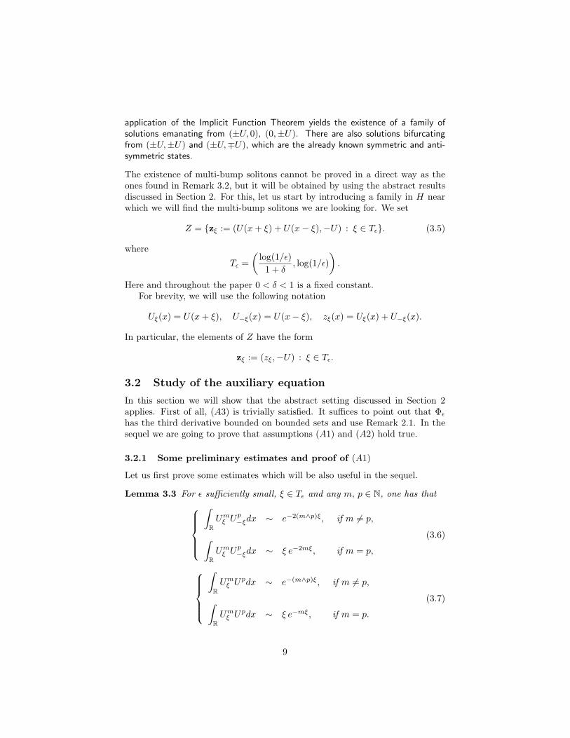
The existence of multi-bump solitons cannot be proved in a direct way as theones found in Remark 3.2, but it will be obtained by using the abstract resultsdiscussed in Section 2. For this, let us start by introducing a family in H nearwhich we will find the multi-bump solitons we are looking for. We set

Z = zξ := (U(x+ ξ) + U(x− ξ),−U) : ξ ∈ Tε. (3.5)

where

Tε =(

log(1/ε)1 + δ

, log(1/ε)).

Here and throughout the paper 0 < δ < 1 is a fixed constant.For brevity, we will use the following notation

Uξ(x) = U(x+ ξ), U−ξ(x) = U(x− ξ), zξ(x) = Uξ(x) + U−ξ(x).

In particular, the elements of Z have the form

zξ := (zξ,−U) : ξ ∈ Tε.

3.2 Study of the auxiliary equation

In this section we will show that the abstract setting discussed in Section 2applies. First of all, (A3) is trivially satisfied. It suffices to point out that Φε

has the third derivative bounded on bounded sets and use Remark 2.1. In thesequel we are going to prove that assumptions (A1) and (A2) hold true.

3.2.1 Some preliminary estimates and proof of (A1)

Let us first prove some estimates which will be also useful in the sequel.

Lemma 3.3 For ε sufficiently small, ξ ∈ Tε and any m, p ∈ N, one has that

∫RUm

ξ Up−ξdx ∼ e−2(m∧p)ξ, if m 6= p,

∫RUm

ξ Up−ξdx ∼ ξ e−2mξ, if m = p,

(3.6)

∫RUm

ξ Updx ∼ e−(m∧p)ξ, if m 6= p,

∫RUm

ξ Updx ∼ ξ e−mξ, if m = p.

(3.7)

9

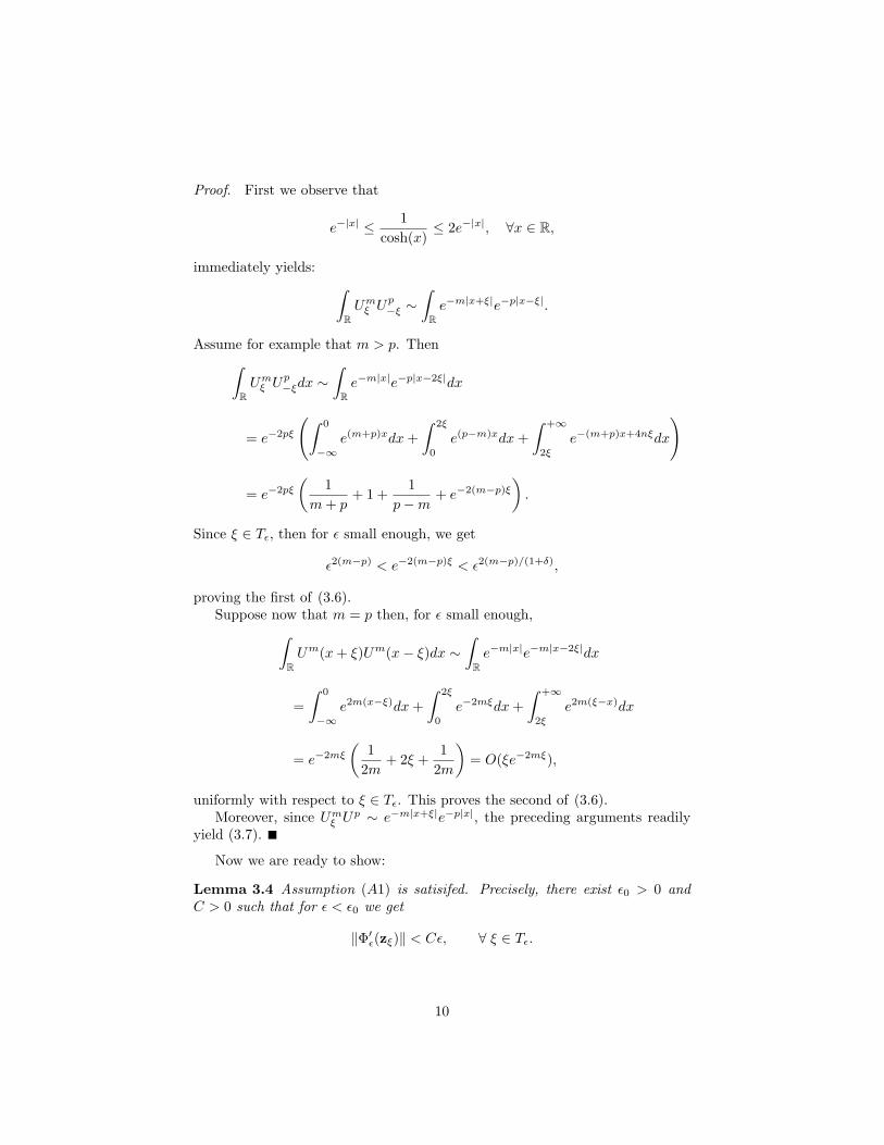
Proof. First we observe that

e−|x| ≤ 1cosh(x)

≤ 2e−|x|, ∀x ∈ R,

immediately yields: ∫RUm

ξ Up−ξ ∼

∫Re−m|x+ξ|e−p|x−ξ|.

Assume for example that m > p. Then∫RUm

ξ Up−ξdx ∼

∫Re−m|x|e−p|x−2ξ|dx

= e−2pξ

(∫ 0

−∞e(m+p)xdx+

∫ 2ξ

0

e(p−m)xdx+∫ +∞

2ξ

e−(m+p)x+4nξdx

)

= e−2pξ

(1

m+ p+ 1 +

1p−m

+ e−2(m−p)ξ

).

Since ξ ∈ Tε, then for ε small enough, we get

ε2(m−p) < e−2(m−p)ξ < ε2(m−p)/(1+δ),

proving the first of (3.6).Suppose now that m = p then, for ε small enough,∫

RUm(x+ ξ)Um(x− ξ)dx ∼

∫Re−m|x|e−m|x−2ξ|dx

=∫ 0

−∞e2m(x−ξ)dx+

∫ 2ξ

0

e−2mξdx+∫ +∞

2ξ

e2m(ξ−x)dx

= e−2mξ

(1

2m+ 2ξ +

12m

)= O(ξe−2mξ),

uniformly with respect to ξ ∈ Tε. This proves the second of (3.6).Moreover, since Um

ξ Up ∼ e−m|x+ξ|e−p|x|, the preceding arguments readily

yield (3.7).

Now we are ready to show:

Lemma 3.4 Assumption (A1) is satisifed. Precisely, there exist ε0 > 0 andC > 0 such that for ε < ε0 we get

‖Φ′ε(zξ)‖ < Cε, ∀ ξ ∈ Tε.

10

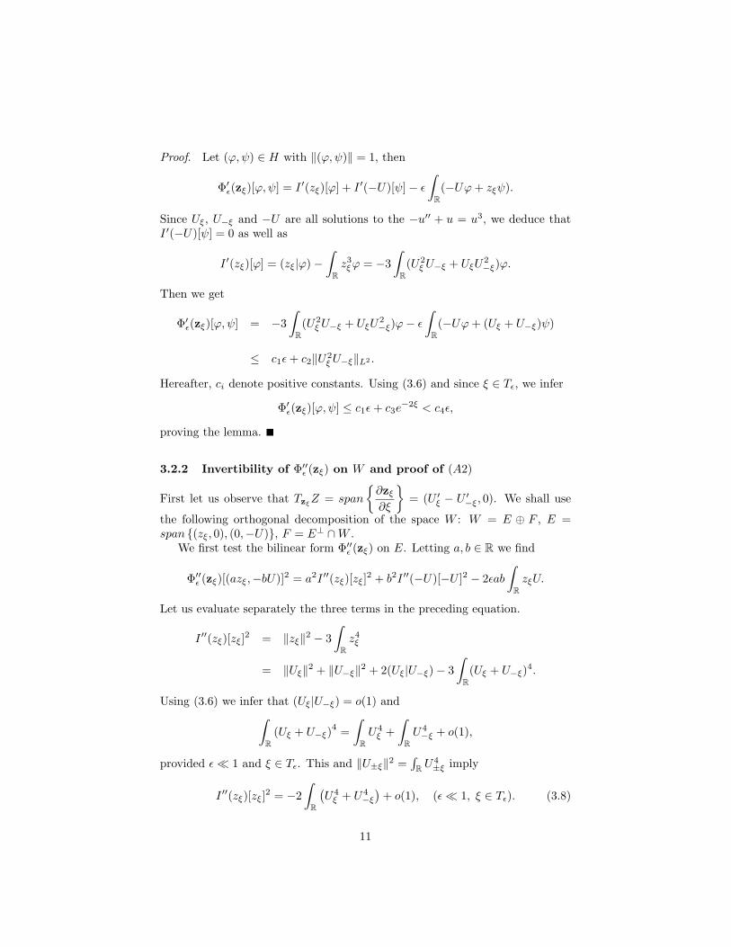
Proof. Let (ϕ,ψ) ∈ H with ‖(ϕ,ψ)‖ = 1, then

Φ′ε(zξ)[ϕ,ψ] = I ′(zξ)[ϕ] + I ′(−U)[ψ]− ε

∫R(−Uϕ+ zξψ).

Since Uξ, U−ξ and −U are all solutions to the −u′′ + u = u3, we deduce thatI ′(−U)[ψ] = 0 as well as

I ′(zξ)[ϕ] = (zξ|ϕ)−∫

Rz3ξϕ = −3

∫R(U2

ξU−ξ + UξU2−ξ)ϕ.

Then we get

Φ′ε(zξ)[ϕ,ψ] = −3∫

R(U2

ξU−ξ + UξU2−ξ)ϕ− ε

∫R(−Uϕ+ (Uξ + U−ξ)ψ)

≤ c1ε+ c2‖U2ξU−ξ‖L2 .

Hereafter, ci denote positive constants. Using (3.6) and since ξ ∈ Tε, we infer

Φ′ε(zξ)[ϕ,ψ] ≤ c1ε+ c3e−2ξ < c4ε,

proving the lemma.

3.2.2 Invertibility of Φ′′ε (zξ) on W and proof of (A2)

First let us observe that TzξZ = span

∂zξ

∂ξ

= (U ′ξ − U ′−ξ, 0). We shall use

the following orthogonal decomposition of the space W : W = E ⊕ F , E =span (zξ, 0), (0,−U), F = E⊥ ∩W .

We first test the bilinear form Φ′′ε (zξ) on E. Letting a, b ∈ R we find

Φ′′ε (zξ)[(azξ,−bU)]2 = a2I ′′(zξ)[zξ]2 + b2I ′′(−U)[−U ]2 − 2εab∫

RzξU.

Let us evaluate separately the three terms in the preceding equation.

I ′′(zξ)[zξ]2 = ‖zξ‖2 − 3∫

Rz4ξ

= ‖Uξ‖2 + ‖U−ξ‖2 + 2(Uξ|U−ξ)− 3∫

R(Uξ + U−ξ)4.

Using (3.6) we infer that (Uξ|U−ξ) = o(1) and∫R

(Uξ + U−ξ)4 =

∫RU4

ξ +∫

RU4−ξ + o(1),

provided ε 1 and ξ ∈ Tε. This and ‖U±ξ‖2 =∫

R U4±ξ imply

I ′′(zξ)[zξ]2 = −2∫

R

(U4

ξ + U4−ξ

)+ o(1), (ε 1, ξ ∈ Tε). (3.8)

11

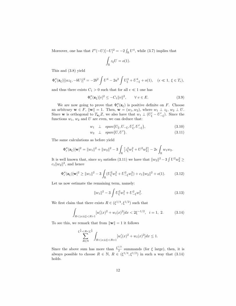
Moreover, one has that I ′′(−U)[−U ]2 = −2∫

R U4, while (3.7) implies that∫

RzξU = o(1).

This and (3.8) yield

Φ′′ε (zξ)[(azξ,−bU)]2 = −2b2∫U4 − 2a2

∫U4

ξ + U4−ξ + o(1), (ε 1, ξ ∈ Tε),

and thus there exists C1 > 0 such that for all ε 1 one has

Φ′′ε (zξ)[v]2 ≤ −C1‖v‖2, ∀ v ∈ E. (3.9)

We are now going to prove that Φ′′ε (zξ) is positive definite on F . Choosean arbitrary w ∈ F , ‖w‖ = 1. Then, w = (w1, w2), where w1 ⊥ zξ, w2 ⊥ U .Since w is orthogonal to Tzξ

Z, we also have that w1 ⊥ (U ′ξ − U ′−ξ). Since thefunctions w1, w2 and U are even, we can deduce that:

w1 ⊥ spanUξ, U−ξ, U′ξ, U

′−ξ, (3.10)

w2 ⊥ spanU,U ′. (3.11)

The same calculations as before yield

Φ′′ε (zξ)[w]2 = ‖w1‖2 + ‖w2‖2 − 3∫

R

[z2ξw

21 + U2w2

2

]− 2ε

∫Rw1w2.

It is well known that, since w2 satisfies (3.11) we have that ‖w2‖2− 3∫U2w2

2 ≥c1‖w2‖2, and hence

Φ′′ε (zξ)[w]2 ≥ ‖w1‖2 − 3∫

R(U2

ξw21 + U2

−ξw21) + c1‖w2‖2 + o(1). (3.12)

Let us now estimate the remaining term, namely:

‖w1‖2 − 3∫U2

ξw21 + U2

−ξw21. (3.13)

We first claim that there exists R ∈ (ξ1/4, ξ1/2) such that∫R<|x±ξ|<R+1

[w′i(x)2 + wi(x)2]dx < 2ξ−1/2, i = 1, 2. (3.14)

To see this, we remark that from ‖w‖ = 1 it follows

ξ14 <R<ξ

12∑

R∈N

∫R<|x±ξ|<R+1

[w′i(x)2 + wi(x)2]dx ≤ 1.

Since the above sum has more than ξ1/2

2 summands (for ξ large), then, it isalways possible to choose R ∈ N, R ∈ (ξ1/4, ξ1/2) in such a way that (3.14)holds.

12

Let us fix an R such that (3.14) holds and define the smooth cut-off functionsχξ, χ−ξ, χ0 : R → [0, 1] by setting

χξ(x) =

1 x > ξ −R,0 x < ξ −R− 1,|χ′ξ(x)| ≤ 2 x ∈ R,

χ−ξ(x) = χξ(−x), χ0 = 1− χ−ξ − χξ.

Let us remark that χ0 satisfies:

χ0(x) =

1 |x| < ξ −R− 1,0 |x| > ξ −R,|χ′0(x)| ≤ 2. x ∈ R

Let us decompose: w1 = vξ + v0 + v−ξ, where

v±ξ = w1χ±ξ, v0 = w1χ0.

From (3.14) it follows (vξ|v0) = o(1), (v−ξ|v0) = o(1), (vξ|v−ξ) = o(1), andthus

‖w1‖2 = ‖vξ‖2 + ‖v0‖2 + ‖v−ξ‖2 + o(1).

Using again (3.14), we obtain

(Uξ|v0) = o(1), (Uξ|v−ξ) = o(1).

Since w1 ⊥ Uξ, one gets that (Uξ|vξ) = o(1). Analogously,

(U−ξ|v0) = o(1), (U−ξ|vξ) = o(1) ⇒ (U−ξ|v−ξ) = o(1),(U ′ξ|v0) = o(1), (U ′ξ|v−ξ) = o(1) ⇒ (U ′ξ|vξ) = o(1),

(U ′−ξ|v0) = o(1), (U ′−ξ|vξ) = o(1) ⇒ (U ′−ξ|v−ξ) = o(1).

This allows us to find a first estimate of (3.13):

‖w1‖2−3∫

RU2

ξw21+U2

−ξw21 = ‖vξ‖2+‖v0‖2+‖v−ξ‖2−3

∫R(U2

ξ v2ξ+U2

−ξv2−ξ)+o(1).

It is now convenient to make a further decomposition, by setting vξ = vξ + vξ,where vξ ∈ spanUξ, U

′ξ and vξ ∈ spanUξ, U

′ξ⊥. Since (Uξ|vξ) = o(1) and

(U ′ξ|vξ) = o(1), see before, we infer that ‖vξ‖ = o(1), yielding

‖vξ‖2 − 3∫U2

ξ v2ξ = ‖vξ‖2 − 3

∫U2

ξ v2ξ + o(1).

Moreover, since vξ ⊥ spanUξ, U′ξ, it follows (see Lemma 3.1)

‖vξ‖2 − 3∫U2

ξ v2ξ ≥ c2‖vξ‖2 ≥ c3‖vξ‖2,

13

and therefore we get

‖vξ‖2 − 3∫U2

ξ v2ξ ≥ c3‖vξ‖2 + o(1). (3.15)

Similarly, we find

‖v−ξ‖2 − 3∫U2−ξv

2−ξ ≥ c4‖v−ξ‖2 + o(1). (3.16)

Substituting (3.15) and (3.16) into (3.13) we finally infer

‖w1‖2−3∫U2

ξw21+U2

−ξw21 ≥ c3‖vξ‖2+c4‖v−ξ‖2+‖v0‖2+o(1) ≥ c5‖w1‖2+o(1).

From this and (3.12) we deduce there exists c6 > 0 such that for all ε 1 andall ξ ∈ Tε one has:

Φ′′ε (zξ)[w]2 ≥ c6‖w‖2.

In conclusion we have proved

Lemma 3.5 There exists a positive constant γ such that for ε small enough andξ ∈ Tε, PΦ′′ε (zξ) is uniformly invertible and there results ‖[PΦ′′ε (zξ)]−1‖ ≤ γ.In other words, (A2) holds.

3.3 Proof of Theorem 1.1

The previous arguments allow us to use Lemma 2.2 which yields a solutionwε,ξ of the auxiliary equation. It remains to find a critical point of the reducedfunctional. For this it is useful the following lemma which provides an expansionof Φε(ξ).

Lemma 3.6 There exist positive constants C,C,C > 0 such that

Φε(ξ) = C − aε,ξe−2ξ + bε,ξ ε ξ e

−ξ +O(ε2), ∀ξ ∈ Tε, ε ∼ 0,

where aε,ξ, bε,ξ ∈ [C,C].

Proof. Since the norm of Φ′′ε is uniformly bounded, we get

Φε(z + w) = Φε(zξ) + Φ′ε(z)[wε,ξ] + O(‖wε,ξ‖2).

First, we are going to neglect the terms of order ε2. In this way, we are goingto prove that the influence of wε,ξ in the reduced functional, Φε, is not relevantin order to find critical points. Observe that by Lemma 3.4 and (2.5) we havethat, for ε 1,

‖Φ′ε(zξ)[wε,ξ]‖ ≤ c1ε2, ∀ ξ ∈ Tε.

14

On the other hand,

Φε(zξ) = I(zξ) + I(−U) + ε

∫RzξU

=34

∫RU4 −

∫RU3

ξU−ξ −32

∫RU2

ξU2−ξ + 2ε

∫RUξU.

Now we study the behavior of each term in the above decomposition. The firstterm is constant, i.e.,

c = 34

∫U4, (3.17)

while Lemma 3.3 yields ∫RU2

ξU2−ξ ∼ ξe−4ξ.

Since ξ ∈ Tε it follows that there exists c1 > 0 and θ > 0 such that for ε 1one has ∣∣∣∣∫ U2

ξU2−ξ

∣∣∣∣ ≤ c1ε−(2+θ)ξ, ∀ ξ ∈ Tε.

On the other hand, using once again Lemma 3.3 we get

−∫

RU3

ξU−ξ ∼ −e−2ξ, 2ε∫

RUξU ∼ εξe−ξ, (3.18)

and the lemma follows.

Proof of Theorem 1.1 completed. According to the previous discussion, to com-plete the proof of Theorem 1.1 it remains to show

Lemma 3.7 For ε sufficiently small, the reduced functional Φε possesses a crit-ical point ξ∗(ε) ∈ Tε.

Proof. Let f(ξ) = −c1e−2ξ +c2ε ξ e−ξ, c1, c2 > 0. By an elementary calculationone finds that f has a strict maximum at ξε such that

e−ξε

ξε − 1=

c22c1

ε. (3.19)

Observe that for all ξ 1 there holds

e−(1+δ)ξ ≤ 2c1c2

e−ξ

ξ − 1≤ e−ξ. (3.20)

Since from (3.19) it follows that ξε → +∞ as ε → 0, then ξε satisfies (3.20)provided ε 1 and hence

− 11 + δ

log ε < ξε < − log ε.

15

Let us evaluate f at ξε and at the extrema of Tε. One has

f(ξε) =c224c1

ε2(ξ2ε − 1) > c3 ε2 log2(1/ε), (ε 1).

On the other hand, taking ζε = − 11+δ log ε and ζ ′ε = − log ε, one has

f(ζε) = −c1ε2

1+δ + c2ζεε2+δ1+δ ∼ −ε

21+δ < 0, as ε→ 0,

as well as

f(ζ ′ε) = −c1ε2 + c2ε2ζ ′ε < c2 ε

2 log(1/ε), (ε 1).

Lemma 3.6 together with the above estimates imply the existence of a maximumfor Φε at a certain ξ∗(ε) ∈ (ζε, ζ ′ε) = Tε, provided ε is sufficiently small. Thiscompletes the proof of Theorem 1.1.

Remark 3.8 One can try to repeat the preceding arguments in order to find so-lutions whose first component has k bumps, k > 2, while the second componentis negative and has h bump(s), h ≥ 1. Unfortunately, the procedure fails becausethe reduced functional has no critical point. We suspect that there are no solutionat all having the first component with more than two bumps. This is confirmed bythe numerical computation in [2].

The preceding observation also highlights the difference between our results andthose of [9]. In that paper, solutions with infinitely many bumps are found. Theiridea is to use two given homoclinics satisfying certain geometrical properties, toconstruct multi-bump solutions by means of a gluing procedure. Observe that, ina sense, we are also gluing the homoclinics (Uξ, 0), (0,−U) and (U−ξ, 0), but theynot verify the conditions assumed in [9].

3.4 Systems with more than two equations

In this section the results found above will be extended to systems with morethan two NLS equations. They arise when one considers the propagation ofpulses in a m-core couplers with circular symmetry. To simplify notation, wewill consider the case m = 3, only. The general case is similar. Setting u =(u1, u1, u3) ∈ H := X ×X ×X, we consider a system like −u′′1 + u1 − u3

1 = ε(u2 + u3),−u′′2 + u2 − u3

2 = ε(u1 + u3),−u′′3 + u3 − u3

3 = ε(u1 + u2),(3.21)

whose corresponding functional is given by

Φε(u) = I(u1) + I(u2) + I(u3)− ε

∫R

[u1u2 + u1u3 + u2u3] dx.

Of course, any triple in which one component is zero and the other two satisfy(1.5), is a solution of (3.21). In addition, dealing with solutions having all threecomponents different from zero, we shall distinguish various other solutions.According to the notation introduced in [3], we consider:

16

• A-type solutions, branching off from solutions with one zero componentwhile the remaining two components are equal, like (U,U, 0).

Focusing, for example, on the family emanating from (U,U, 0), the correspondinglinearized system is −φ′′1 + φ1 − 3U2φ1 = 0,

−φ′′2 + φ2 − 3U2φ2 = 0,−φ′′3 + φ3 = 0.

(3.22)

The same arguments carried out in Remark 3.2 show that (U,U, 0) is non-degenerate and hence there exists a family of solutions uε ∈ H, whose compo-nents satisfy

uj,ε ∼ U, (j = 1, 2), u3,ε ∼ 0, (ε→ 0). (3.23)

Another kind of solutions is given by the

• B-type solutions, which have one multi-bump component, a second com-ponent near −U , a third near 0.

The existence of this type of solutions can be proved by the same argumentsused in Theorem 1.1. We will focus on the particular case (the other ones,obtained by permutation of the indices 1, 2, 3, are quite similar) in which onehas:

u1,ε ∼ Uξ + U−ξ, u2,ε ∼ −U, u3,ε ∼ 0, (ε→ 0). (3.24)

These solutions bifurcate from the manifold

ZB = zξ := (Uξ + U−ξ,−U, 0) : ξ ∈ Tε

which has exactly the same properties of Z defined in (3.5). Therefore, repeatingthe same arguments used for Theorem 1.1, one can prove the existence of theB-type solutions.

Next, we are going to consider solutions which have all the three componentsfar from zero. The first family is the

• C1-type solutions, which have the components satisfying, for example,

uj,ε ∼ U, (j = 1, 2), u3,ε ∼ −U, (ε→ 0). (3.25)

The existence of these solutions follows immediately applying the Implicit func-tion Theorem, as for theA-type solutions. Actually, (U,U,−U) is non-degeneratein the space H. A second family consists of the

• C2-type solutions, which have two multi-bump components, while the thirdone is near −U .

17

As for the B-type solutions, the existence of the C2-type solutions can be provedby the same arguments used in Theorem 1.1. Let us focus, for example, onsolutions such that

uj,ε ∼ Uξ + U−ξ, (j = 1, 2), u3,ε ∼ −U, (ε→ 0). (3.26)

The corresponding manifold is

ZC = zξ := (Uξ + U−ξ, Uξ + U−ξ,−U) : ξ ∈ Tε.

Here we work on the space

H = u ∈ X ×X ×X : u1 = u2.

According to the Symmetric Criticality Principle, see [20] or [23, Theorem 1.28],the critical points of Φε on H are critical points of Φε and hence solutions of(3.21). Carrying out similar arguments as in the proof of Theorem 1.1, we areled to study the reduced functional, whose leading part is, as before Φε(zξ). Inthe present case one finds

Φ(zξ) = 2I(Uξ + U−ξ) + I(−U)− ε

∫R

[−2U(Uξ + U−ξ) + (Uξ + U−ξ)2

]dx,

One has:2I(Uξ + U−ξ) + I(−U) ∼ c′ − 2 e−2ξ,

as well as

ε

∫R

2U(Uξ + U−ξ)dx− ε

∫R(Uξ + U−ξ)2dx

= 4ε∫

RUξUdx− 2ε

∫RU2

ξ dx− 2∫

RUξU−ξdx

∼ 4ε ξ e−ξ − c′′ ε− 2ε ξ e−2ξ.

Thus, setting c∗ = c′ − c′′ε we get

Φε(ξ) ∼ c∗ − 2 e−2ξ + 4ε ξ e−ξ +O(ε2), ∀ ξ ∈ Tε,

which is nothing but Lemma 3.6. It follows that we can repeat once more thearguments of Lemma 3.7 to infer the existence of C2-type solutions.

Finally, there exists a last family, different from all the previous ones:

• E-type solutions, such that u1,ε(x) = u2,ε(−x) and u3,ε(x) = u3,ε(−x).

More precisely, we will find solutions of the type u1,ε ∼ Uξ, u2,ε ∼ U−ξ andu3,ε ∼ −U(x). Let us remark explicitly that the first two components areasymmetric with respect to x. To prove the existence of E-type solutions we

18

will use again the perturbation method, but in a way different than in theprevious cases. First of all, we shall work on the space

H = u ∈ E × E × E : u1(x) = u2(−x), u3(x) = u3(−x), E = W 1,2(R).

Using again the Symmetric Criticality Principle, the critical points of Φε on Hsolutions of (3.21). Let us consider the manifold

ZE = zξ = (Uξ, U−ξ,−U) ∈ H : ξ ∈ R.

Clearly any zξ ∈ ZE is a critical point of Φ0. Moreover, as for (3.22), onehas that (φ1, φ2, φ3) ∈ KerΦ′′0(zξ) if and only if φ1 = aU ′ξ, φ2 = b U ′−ξ, andφ3 = cU ′ for some a, b, c ∈ R. Then the requirement that (φ1, φ2, φ3) ∈ Himplies a = −b and c = 0. Therefore, Ker[Φ′′0(zξ)] = T ezξ

ZE , namely ZE is anon-degenerate critical manifold, see [6, Section 2.2]. Set

Γ(ξ) = −∫

RG(zξ)dx = −

∫RUUξdx−

∫RUU−ξdx+

∫RUξU−ξdx.

According to [6, Thm. 2.16], see also Remark 2.5, any maximum or minimumξ of Γ gives rise to a critical point uε of Φε such that uε → zeξ as ε → 0. By adirect computation it follows that

Γ(0) < 0, Γ′(0) = 0, Γ′′(0) < 0.

Therefore there exists ξ > 0 such that Γ has a minimum at ±ξ. Thus we inferthat (3.21) possesses, for ε sufficiently small, a family of solutions uε of type E.Precisely, the components of uε satisfy:

u1,ε → Ueξ, u2,ε → U−eξ, u3,ε → −U, (ε→ 0). (3.27)

Summarizing, we can state the following result:

Theorem 3.9 For ε sufficiently small, the system (3.21) has the following so-lutions:

(a) A-type solutions, whose components satisfy (3.23) (and its permutations);

(b) B-type solutions, whose components satisfy (3.24) (and its permutations);

(c1) C1-type solutions, whose components satisfy (3.25) (and its permutations);

(c2) C2-type solutions, whose components satisfy (3.26) (and its permutations);

(e) E-type solutions, whose components satisfy (3.27) (and its permutations).

Remark 3.10 The system considered in [3] is slightly different than (3.21), be-cause the left hand side is −u′′j + quj − u3

j , q being a real parameter. This makestheir results not directly comparable with ours. For example, dealing with the E-type solutions, there is a numerical evidence (see [3, Figure 9.3]) that the peaks ofthe two positive components should tend to zero when the bifurcation parameterq/ε ≈ 2.747, while we have shown that they converge to ±ξ as ε → 0, see point(e) before.

19

4 The PDE case

In this part we are concerned with the proof of Theorem 1.3. To cover alsothe case of two bumps solutions, it is understood that the polytope P may alsodenote the degenerate polygon with two vertices, which are symmetric withrespect to the origin (in such case s = 2, r = 1).

Let G be the polyedral group associated to P, namely the group of all isome-tries that leave invariant P, see [11, pag. 46]. The Sobolev space of functionswhich are invariant under G, will be denoted by

X = u ∈W 1,2(Rn) : u g = u a.e. in Rn , ∀g ∈ G

We will work in H = X × X and consider the functional Φε : H → R,

Φε(u) = I(u1) + I(u2)− εΨ(u), u = (u1, u2),

whereI(u) =

12‖u‖2 − 1

4

∫u4dx, Ψ(u) =

∫u1u2dx,

and‖u‖2 =

∫(|∇u|2 + u2)dx.

We also denote by (u | v) =∫

(∇u ·∇v+uv)dx the scalar product in W 1,2(Rn),corresponding to the preceding norm.

Since X = Fix(G), the Palais Symmetric Criticality Principle implies thatthe critical points of Φε on H correspond to solutions of (1.7).

Let us remark that when P is the degenerate polytope with two symmetricpoints, the preceding theorem is nothing but the extension of Theorem 1.1 inRn, n = 2, 3.

In the proof of Theorem 1.3 we follow the same abstract approach as inthe ODE case. However, as anticipated in the Introduction, the proof of thistheorem requires some new ingredients. Since here the distance of the peaks tothe origin is larger, the interaction among the bumps is weaker, and then weneed better estimates for the reduced functional. To overcome this problem,we will consider a manifold Z which approximates the solutions we are lookingfor more accurately. This yields sharper estimates and allows us to obtain theconclusion. For this purpose, in the next Subsection, we will first construct apair (Vε, vε) ∈ H bifurcating from (U, 0) where U denotes the unique positiveradial solution of −∆u+ u = u3, in W 1,2(Rn), see Lemma 3.1.

4.1 Bifurcation from (U, 0)

Consider the problem −∆u+ u− u3 = εv,−∆v + v − v3 = εu,

(4.1)

where we assume u, v ∈ H1r (Rn), n = 2, 3. For ε = 0 there is a solution of the

form (U, 0), where U denotes the unique positive radial solution of−∆u+u = u3.In next proposition we obtain bifurcation on the parameter ε from this solution.

20

Proposition 4.1 There exists ε0 > 0 and a C∞ curve

(−ε0, ε0) → (Vε, vε) ∈ H2r (Rn)×H2

r (Rn),

of solutions of (4.1). Moreover, (V0, v0) = (U, 0).

Proof. Define F : H2r (Rn)×H2

r (Rn)× R → L2r(Rn)× L2

r(Rn),

F (u, v, ε) =(−∆u+ u− u3 − εv−∆v + v − v3 − εu

).

Obviously, the solutions of (4.1) correspond to the zeroes of F . We plan toobtain local bifurcation from (U, 0) by means of the Implicit Function Theorem.Clearly one has:

• F ∈ C∞,

• F (U, 0, 0) = (0, 0),

• ∂u,vF (U, 0, 0)[ϕ,ψ] = (−∆ϕ+ ϕ− 3U2ϕ,−∆ψ + ψ).

We now verify that this operator is invertible, that is, given (f, g) ∈ L2r(Rn) ×

L2r(Rn), the problem

−∆ϕ+ ϕ− 3U2ϕ = f−∆ψ + ψ = g

(4.2)

has a solution in H2r (Rn)×H2

r (Rn).Clearly, the second equation of (4.2) is uniquely solvable. Moreover, the

Fredholm Alternative and Lemma 3.1 imply that also the first equation isuniquely solvable in H1

r (Rn). Therefore, there exist (ϕ,ψ) ∈ H1r (Rn)×H1

r (Rn)solving (4.2). Finally, they are in H2(Rn) because of the regularity resultof Agmon-Douglis-Nirenberg [1]. Hence, the Implicit Function Theorem im-plies the existence of a C∞ curve ε 7→ (Vε, vε) ∈ H2

r (Rn) × H2r (Rn) such that

F (Vε, vε, ε) = 0.

Recall for further purposes that:

‖Vε − U‖H2 → 0, ‖vε‖H2 → 0 as ε→ 0. (4.3)

As we shall see, we will use the functions Vε, vε to construct the manifold ofapproximated solutions. In order to deal with these functions, we will need touse their Taylor expansion in ε:

Vε = U + εw1 + ε2

2 w2 + . . .

vε = εw1 + ε2

2 w2 + . . .

In order to compute wk, wk, k = 1, 2, . . . , we just make the derivative of:−∆Vε + Vε − V 3

ε = εvε,−∆vε + vε − v3

ε = εVε,

21

with respect to ε. Then, denoting by a ”dot” the derivative with respect to ε,we find

−∆Vε + Vε − 3V 2ε Vε = vε + εvε,

−∆vε + vε − 3v2ε vε = Vε + εVε.

For ε = 0 we get −∆w1 + w1 − 3U2w1 = 0,

−∆w1 + w1 = U.

In particular w1 = 0. Taking the second derivative with respect to ε we obtainthat

−∆Vε + Vε − 3[2VεV2

ε + V 2ε Vε] = 2vε + εvε,

−∆vε + vε − 3[2vεv2ε + v2

ε vε] = 2Vε + εVε,

hence for ε = 0 we find that−∆w2 + w2 − 3U2w2 = 2w1,

−∆w2 + w2 = 2w1 = 0.

In particular w2 = 0. In general,−∆wk + wk −

dk

dεk

∣∣∣ε=0

(V 3ε ) = kwk−1,

−∆wk + wk −dk

dεk

∣∣∣ε=0

(v3ε) = kwk−1.

(4.4)

In (4.4) one has that for l,m, i, j, s nonnegative integers:

dk

dεk

∣∣∣ε=0

(V3ε) = k!

∑l 6=m

2l+m=k

3w2l wm

(l!)2m!+

∑i6=j 6=s 6=ii+j+s=k

6wiwjws

i!j!s!+ f(k)

w3k/3

(k/3)!,

(4.5)

where f(k) = 1 if k/3 ∈ N, f(k) = 0 on the contrary. An analogous expression

holds fordk

dεk

∣∣∣ε=0

(v3ε ).

Lemma 4.2 wk = 0 if k is odd and wk = 0 if k is even.

Proof. We argue by induction. For k = 0, 1, 2 the result holds. Suppose thatit holds for every t < k.

1. Assume k is odd. In such case, observe that in (4.5) any summand has afactor wp with p odd. Moreover, all these p’s are smaller than k, exceptthe term with l = 0, m = k. Then the expression (4.5) will be equal to3U2wk. Inserting this into the first equation of (4.4) we have:

−∆wk + wk − 3U2wk = kwk−1.

By induction, wk−1 = 0 which implies that wk = 0.

22

2. Assume that k is even. Arguing in the same way as above, we obtain thatwk verifies:

−∆wk + wk = kwk−1.

By induction, wk−1 = 0 and hence we infer that wk = 0.

Now we establish the decay of the functions wk and wk. The following lemmawill be useful.

Lemma 4.3 Assume that f(x) = f(|x|) is a radial function verifying that|f(r)| ≤ Crαr

1−n2 e−r, ∀ r > 1, where α > −1 and C > 0. Let u ∈ H1

r (Rn)be the solution of the equation −∆u+ u = f . Then |u(r)| ≤ C ′rα+1r

1−n2 e−r.

Proof. Writing the equation −∆u+ u = f in radial coordinates we obtain−u′′ − (n− 1)u′

r + u = f(r)limr→∞ u(r) = 0.

First, consider the homogeneous equation −u′′ − n−1r u′ + u = 0. The set of

solutions is a two dimensional vector space generated by u1, u2, which aredefined as:

u1(r) = r2−n

2 BK

(n− 2

2, r

), u2(r) = r

2−n2 BI

(n− 2

2, r

).

In the above expressionsBK , BI are the modified Bessel functions of the first andsecond type respectively, see [14]. From the properties of the Bessel functionswe have u1(r) ∼ r

1−n2 e−r, u2(r) ∼ r

1−n2 er.

GivenR, A fixed constants and f a fixed function, the solution of the problem−u′′ − (n− 1)u′

r + u = fu(R) = A, limr→∞ u(r) = 0

can be obtained by the variation of constants formula:

u(r) = u1(r)∫ r

R

u2(s)f(s)sn−1ds+ u2(r)∫ r

R

u1(s)f(s)sn−1ds+ au1(r) + bu2(r)

for some real constants a, b. Let us study the first summand in the aboveexpression:∣∣∣∣u1(r)

∫ r

R

u2(s)f(s)sn−1ds

∣∣∣∣ ≤ u1(r)∫ r

R

u2(s)|f(s)|sn−1ds

≤∫ r

R

u1(s)u2(s)|f(s)|sn−1ds ∼∫ r

R

|f(s)|ds <∫ +∞

R

|f(s)|ds <∞.

23

Therefore, by using that limr→∞ u(r) = 0, we conclude that

b = −∫ +∞

R

u1(s)f(s)sn−1ds.

Hence, we can rewrite u as follows:

u(r) = u1(r)∫ r

R

u2(s)f(s)sn−1ds+ u2(r)∫ +∞

r

u1(s)f(s)sn−1ds+ au1(r),

where the constant a is given by the boundary condition u(R) = A. We provenow the decay of u:∣∣∣∣ u(r)

rα+1u1(r)

∣∣∣∣ ≤ 1rα+1

∫ r

R

u2(s)|f(s)|sn−1

+u2(r)

rα+1u1(r)

∫ +∞

r

u1(s)|f(s)|sn−1ds+a

rα+1.

We study each term separately:

1rα+1

∫ r

R

u2(s)|f(s)|sn−1ds ≤ C

rα+1

∫ r

R

sαds =C

rα+1

rα+1 −Rα+1

α+ 1≤ C

α+ 1.

u2(r)rα+1u1(r)

∫ +∞

r

u1(s)|f(s)|sn−1ds ≤ Ce2r

rα+1

∫ +∞

r

sαe−2sds.

Using thater

rαis increasing for r ≥ r0 we get:

e2r

rα+1

∫ +∞

r

sαe−2sds =er

r

er

rα

∫ +∞

r

sαe−2sds

≤ er

r

∫ +∞

r

es

sαsαe−2sds =

er

r

∫ +∞

r

e−sds =1r.

As a consequence,

u2(r)rα+1u1(r)

∫ +∞

r

u1(s)|f(s)|sn−1ds→ 0 as r → +∞.

So the result follows.

Remark 4.4 The same arguments used before imply that:

• If α = −1 then u(r) ≤ C ′ log(r)r1−n

2 e−r.

• If α < −1 then u(r) ≤ C ′r1−n

2 e−r.

24

The above estimates are sharp, as can be easily checked in the one dimen-sional case (n = 1).

Corollary 4.1 The functions wk, wk satisfy the estimate:

|wk(r)|, |wk(r)| ≤ Ckrkr

1−n2 e−r for r > 1, Ck > 0. (4.6)

Proof. We argue by induction. Clearly for k = 0 (4.6) holds. Suppose (4.6)holds for any m < k.

First, consider the function wk which satisfies (see the first equation in (4.4))

−∆wk + wk = kwk−1 + Yk,

where Yk denotes the right hand side of (4.5). Now let us remark that thedecay of kwk−1 is at most like rk−1r

1−n2 e−r, while the one of Yk is stronger.

Actually, 3U2wk, corresponding to the first term in (4.5) with l = 0,m = k,decays like r1−ne−2rwk, while all the remaining terms contain three factorswj , j < k. Therefore, wk solves an equation of type −∆wk + wk = f where|f(r)| ≤ C ′k−1r

k−1r1−n

2 e−r. By Lemma 4.3 the conclusion follows.In a similar way we can argue with the function wk.

4.2 The approximate solutions: proof of (A1)

Given i ∈ 1 . . .m, ε > 0 small and ξ ∈ R, define:

Vi(x) = V iε,ξ(x) = Vε(x− ξpi) , vi(x) = vi

ε,ξ(x) = vε(x− ξpi)

where Vε, vε are the functions found in Subsection 4.1. Sometimes we will writeVi, vi with a double purpose: for short, and not to confuse with powers.

In the sequel, we will always assume that ξ is a parameter satisfying (1.9),where δ > 0 is a small positive constant to be chosen.

Letz1 = z1(ε, ξ) := V 1

ε,ξ + · · ·+ V mε,ξ − vε

andz2 = z2(ε, ξ) := v1

ε,ξ + · · ·+ vmε,ξ − Vε.

Since Vε and vε are radial, it follows that zi ∈ X , i = 1, 2. Let us define thefollowing manifold of approximate solutions:

Z = zε,ξ = (z1(ε, ξ), z2(ε, ξ)) : ξ ∈ Tε.

Remark 4.5 The solutions (u1,ε, u2,ε) of Theorem 1.3 will bifurcate from suitablepoints of Z and thus have the following asymptotic behavior:

- u1,ε ∼ z1(ε, ξ) = V 1ε,ξ + · · ·+ V m

ε,ξ − vε ∼∑U(·+ ξpi),

- u2,ε ∼ z2(ε, ξ) = v1ε,ξ + · · ·+ vm

ε,ξ − Vε ∼ −U .

25

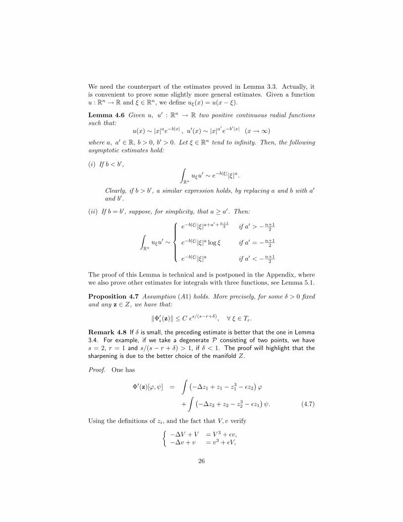
We need the counterpart of the estimates proved in Lemma 3.3. Actually, itis convenient to prove some slightly more general estimates. Given a functionu : Rn → R and ξ ∈ Rn, we define uξ(x) = u(x− ξ).

Lemma 4.6 Given u, u′ : Rn → R two positive continuous radial functionssuch that:

u(x) ∼ |x|ae−b|x| , u′(x) ∼ |x|a′e−b′|x| (x→∞)

where a, a′ ∈ R, b > 0, b′ > 0. Let ξ ∈ Rn tend to infinity. Then, the followingasymptotic estimates hold:

(i) If b < b′, ∫Rn

uξu′ ∼ e−b|ξ||ξ|a.

Clearly, if b > b′, a similar expression holds, by replacing a and b with a′

and b′.

(ii) If b = b′, suppose, for simplicity, that a ≥ a′. Then:

∫Rn

uξu′ ∼

e−b|ξ||ξ|a+a′+ n+1

2 if a′ > −n+12

e−b|ξ||ξ|a log ξ if a′ = −n+12

e−b|ξ||ξ|a if a′ < −n+12

The proof of this Lemma is technical and is postponed in the Appendix, wherewe also prove other estimates for integrals with three functions, see Lemma 5.1.

Proposition 4.7 Assumption (A1) holds. More precisely, for some δ > 0 fixedand any z ∈ Z, we have that:

‖Φ′ε(z)‖ ≤ C εs/(s−r+δ), ∀ ξ ∈ Tε.

Remark 4.8 If δ is small, the preceding estimate is better that the one in Lemma3.4. For example, if we take a degenerate P consisting of two points, we haves = 2, r = 1 and s/(s − r + δ) > 1, if δ < 1. The proof will highlight that thesharpening is due to the better choice of the manifold Z.

Proof. One has

Φ′(z)[ϕ,ψ] =∫ (

−∆z1 + z1 − z31 − εz2

)ϕ

+∫ (

−∆z2 + z2 − z32 − εz1

)ψ. (4.7)

Using the definitions of zi, and the fact that V, v verify−∆V + V = V 3 + εv,−∆v + v = v3 + εV,

26

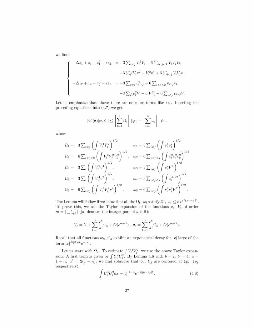
we find:

−∆z1 + z1 − z31 − εz2 = −3

∑i 6=j V

2i Vj − 6

∑i<j<k ViVjVk

−3∑

i(Viv2 − V 2

i v) + 6∑

i<j ViVjv,

−∆z2 + z2 − z32 − εz1 = −3

∑i 6=j v

2i vj − 6

∑i<j<k vivjvk

−3∑

i(v2i V − viV

2) + 6∑

i<j vivjV.

Let us emphasize that above there are no more terms like εzi. Inserting thepreceding equations into (4.7) we get

|Φ′(z)[ϕ,ψ]| ≤

[5∑

l=1

Ωl

]‖ϕ‖+

[5∑

l=1

ωl

]‖ψ‖.

where

Ω1 = 3∑

i 6=j

(∫V 4

i V2j

)1/2

, ω1 = 3∑

i 6=j

(∫v4

i v2j

)1/2

Ω2 = 6∑

i<j<k

(∫V 2

i V2j V

2k

)1/2

, ω2 = 6∑

i<j<k

(∫v2

i v2j v

2k

)1/2

Ω3 = 3∑

i

(∫V 2

i v4

)1/2

, ω3 = 3∑

i 6=j

(∫v2

i V4

)1/2

Ω4 = 3∑

i

(∫V 4

i v2

)1/2

, ω4 = 3∑

i<j<k

(∫v4

i V2

)1/2

Ω5 = 6∑

i<j

(∫V 2

i V2j v

2

)1/2

, ω5 = 6∑

i<j

(∫v2

i v2jV

2

)1/2

.

The Lemma will follow if we show that all the Ωl, ωl satisfy Ωl, ωl ≤ c εs/(s−r+δ).To prove this, we use the Taylor expansion of the functions vε, Vε of orderm = [ s

s−r+δ ] ([a] denotes the integer part of a ∈ R):

Vε = U +m∑

k=1

εk

k!wk +O(εm+1) , vε =

m∑k=1

εk

k!wk +O(εm+1).

Recall that all functions wk, wk exhibit an exponential decay for |x| large of theform |x| 1−n

2 +ke−|x|.

Let us start with Ω1. To estimate∫V 4

i V2j , we use the above Taylor expan-

sion. A first term is given by∫U4

i U2j . By Lemma 4.6 with b = 2, b′ = 4, a =

1 − n, a′ = 2(1 − n), we find (observe that Ui, Uj are centered at ξpi, ξpj

respectively) ∫U4

i U2j dx ∼ |ξ|1−ne−2|pi−pj |ξ. (4.8)

27

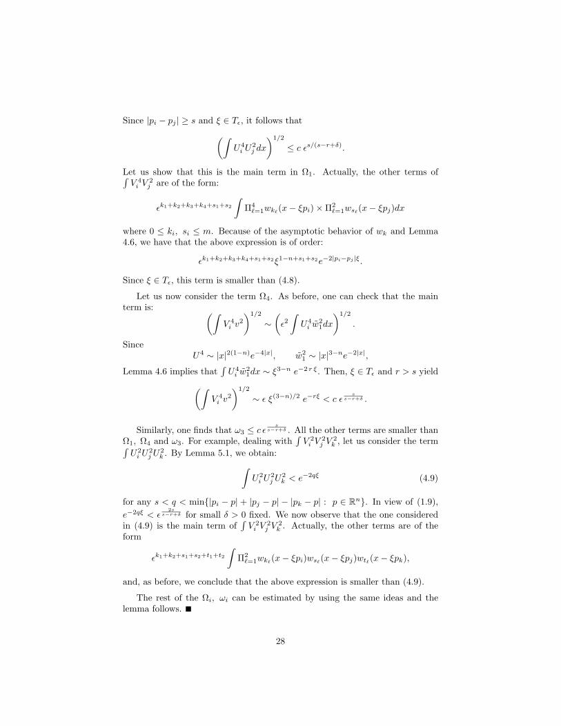
Since |pi − pj | ≥ s and ξ ∈ Tε, it follows that(∫U4

i U2j dx

)1/2

≤ c εs/(s−r+δ).

Let us show that this is the main term in Ω1. Actually, the other terms of∫V 4

i V2j are of the form:

εk1+k2+k3+k4+s1+s2

∫Π4

`=1wk`(x− ξpi)×Π2

`=1ws`(x− ξpj)dx

where 0 ≤ ki, si ≤ m. Because of the asymptotic behavior of wk and Lemma4.6, we have that the above expression is of order:

εk1+k2+k3+k4+s1+s2ξ1−n+s1+s2e−2|pi−pj |ξ.

Since ξ ∈ Tε, this term is smaller than (4.8).

Let us now consider the term Ω4. As before, one can check that the mainterm is: (∫

V 4i v

2

)1/2

∼(ε2∫U4

i w21dx

)1/2

.

SinceU4 ∼ |x|2(1−n)e−4|x|, w2

1 ∼ |x|3−ne−2|x|,

Lemma 4.6 implies that∫U4

i w21dx ∼ ξ3−n e−2 r ξ. Then, ξ ∈ Tε and r > s yield(∫

V 4i v

2

)1/2

∼ ε ξ(3−n)/2 e−rξ < c εs

s−r+δ .

Similarly, one finds that ω3 ≤ c εs

s−r+δ . All the other terms are smaller thanΩ1, Ω4 and ω3. For example, dealing with

∫V 2

i V2j V

2k , let us consider the term∫

U2i U

2j U

2k . By Lemma 5.1, we obtain:∫

U2i U

2j U

2k < e−2qξ (4.9)

for any s < q < min|pi − p| + |pj − p| − |pk − p| : p ∈ Rn. In view of (1.9),e−2qξ < ε

2ss−r+δ for small δ > 0 fixed. We now observe that the one considered

in (4.9) is the main term of∫V 2

i V2j V

2k . Actually, the other terms are of the

form

εk1+k2+s1+s2+t1+t2

∫Π2

`=1wk`(x− ξpi)ws`

(x− ξpj)wt`(x− ξpk),

and, as before, we conclude that the above expression is smaller than (4.9).

The rest of the Ωi, ωi can be estimated by using the same ideas and thelemma follows.

28

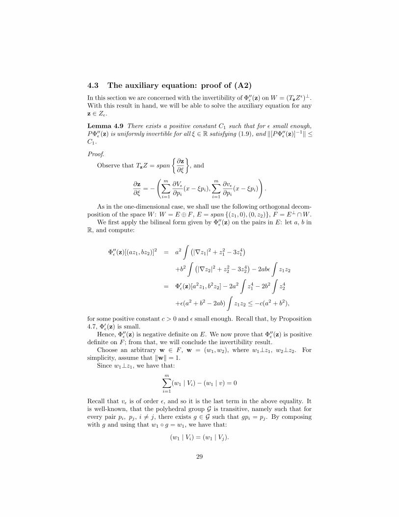
4.3 The auxiliary equation: proof of (A2)

In this section we are concerned with the invertibility of Φ′′ε (z) on W = (TzZε)⊥.

With this result in hand, we will be able to solve the auxiliary equation for anyz ∈ Zε.

Lemma 4.9 There exists a positive constant C1 such that for ε small enough,PΦ′′ε (z) is uniformly invertible for all ξ ∈ R satisfying (1.9), and ‖[PΦ′′ε (z)]−1‖ ≤C1.

Proof.

Observe that TzZ = span

∂z∂ξ

, and

∂z∂ξ

= −

(m∑

i=1

∂Vε

∂pi(x− ξpi),

m∑i=1

∂vε

∂pi(x− ξpi)

).

As in the one-dimensional case, we shall use the following orthogonal decom-position of the space W : W = E ⊕F , E = span (z1, 0), (0, z2), F = E⊥ ∩W .

We first apply the bilineal form given by Φ′′ε (z) on the pairs in E: let a, b inR, and compute:

Φ′′ε (z)[(az1, bz2)]2 = a2

∫ (|∇z1|2 + z2

1 − 3z41

)+b2

∫ (|∇z2|2 + z2

2 − 3z42

)− 2abε

∫z1z2

= Φ′ε(z)[a2z1, b

2z2]− 2a2

∫z41 − 2b2

∫z42

+ε(a2 + b2 − 2ab)∫z1z2 ≤ −c(a2 + b2),

for some positive constant c > 0 and ε small enough. Recall that, by Proposition4.7, Φ′ε(z) is small.

Hence, Φ′′ε (z) is negative definite on E. We now prove that Φ′′ε (z) is positivedefinite on F ; from that, we will conclude the invertibility result.

Choose an arbitrary w ∈ F , w = (w1, w2), where w1⊥z1, w2⊥z2. Forsimplicity, assume that ‖w‖ = 1.

Since w1⊥z1, we have that:m∑

i=1

(w1 | Vi)− (w1 | v) = 0

Recall that vε is of order ε, and so it is the last term in the above equality. Itis well-known, that the polyhedral group G is transitive, namely such that forevery pair pi, pj , i 6= j, there exists g ∈ G such that gpi = pj . By composingwith g and using that w1 g = w1, we have that:

(w1 | Vi) = (w1 | Vj).

29

Therefore, (w1 | Vi) ≤ Cε for all i = 1 . . .m.

Moreover, w is orthogonal to∂z∂ξ

, which implies that:

(w1 |∂z1∂ξ

) + (w2 |∂z2∂ξ

) = 0.

Observe now that∂z2∂ξ

is of order ε, and this means that:

(w1 |∂z1∂ξ

) ≤ Cε.

Take again g ∈ G such that gpi = pj , i 6= j. Reasoning as above, we obtain:(w1 |

∂Vε

∂pi(x− ξpi)

)=(w1 |

∂Vε

∂pj(x− ξpj)

).

Therefore, we conclude that(w1 |

∂Vε

∂pi(x− ξpi)

)≤ Cε, ∀ i = 1 . . . n.

We now claim that w1⊥∂Vε

∂q(x − ξpi) for any q orthogonal to pi (in the Rn

sense). To prove that, we need to make use of the following property of P. Forevery vertex p ∈ P we can find a line ` ⊂ R2, resp. two planes π1 6= π2 ⊂ R3,such that p ∈ `, resp. pj ∈ π1 ∩ π2, and P is symmetric with respect to `, resp.π1 and π2. Such a property is trivially verified for the regular polygons in R2.For the regular polyhedra in R3, it suffices to take two non-planar sides passingthrough p and consider the two planes containing each side and the origin.

Fixed i, take q1, . . . qn−1 ∈ Rn unitary vectors orthogonal to pi, linearlyindependent, and such that P is symmetric with respect to the hyperplane(plane, if n = 3, line, if n = 2):

πj = x ∈ Rn : 〈x, qj〉 = 0.

Let gj be the reflection with respect to πj , that is, gj(x) = x− 2〈x, qj〉qj .Recall now that w1 is G−invariant. Moreover, since Vε is radial, the function:

∂Vε

∂qj(x− ξpi) is odd with respect to qj , that is,

∂Vε

∂qj(gj(x)− ξpi) = −∂Vε

∂qj(x− ξpi).

Therefore, w1⊥∂Vε

∂qj(x− ξpi) for any j = 1 . . . n− 1.

We now focus on w2. Since w2⊥z2, we have that:m∑

i=1

(w2 | vi)− (w2 | V ) = 0.

30

Since vi is of order ε, we have that: (w2 | V ) is also of order ε. Recall that bothw2 and Vε are radial functions; using symmetry arguments as before, one easily

obtains that w2⊥∂Vε

∂xj(x) for any j = 1 . . . n.

As we mentioned before, we claim that Φ′′ε (z)[w,w] > c > 0. Let us compute:

Φ′′ε (z)[w,w] = ‖w1‖2 + ‖w2‖2 −∫ [

3z21w

21 + 3z2

2w22 − 2εw1w2

]dx.

By neglecting the terms which tend to zero, we obtain,

Φ′′ε (z)[w,w] ∼ ‖w1‖2 + ‖w2‖2 − 3∫w2

1

(m∑

i=1

V 2i

)dx− 3

∫V 2w2

2dx. (4.10)

First, recall that since (w2 | V ) = o(1), (w2 |∂Vε

∂xj(x)) = 0, we can use Lemma

3.1 to prove that: ∫|∇w2|2 + w2

2 − 3V 2w22 ≥ c‖w2‖2 − Cε. (4.11)

In order to estimate the remaining part of (4.10), we argue as in the one-dimensional case.Claim: There exists R ∈ (ξ1/4, ξ1/2) such that

m∑j=1

∫R<|x−ξpj |<R+1

[|∇wi|2 + w2i ]dx < 2ξ−1/2, i = 1, 2

The proof of this claim can be done as in the ODE case.

Once we have that constant R, we can define:

χj(x) =

1 |x− ξpj | < R0 |x− ξpj | > R+ 1|∇χj(x)| ≤ 2 ∀x ∈ Rn

Define also χ0(x) = 1−∑m

j=1 χj(x). We can now decompose w1 =∑m

j=0 w1χj

and argue as in the one-dimensional case, to conclude that:∫|∇w1|2 + w2

1 − 3w21

(m∑

i=1

V 2i

)≥ c‖w1‖2 − Cε (4.12)

Estimates (4.12) and (4.11) imply that (4.10) is above a fixed positive con-stant.

31

4.4 Proof of Theorem 1.3

In the previous sections we have proved that (A1) and (A2) hold. Since (A3)is trivially satisfied as in the ODE case, we can use the results of Section 2 toconclude that the auxiliary equation has a solution wε,ξ for ε small and any ξsatisfying (1.9).

So, we are led with the study of critical points of the reduced functional,that is, the function:

Φε(ξ) = Φε(zε,ξ + wε,ξ).

We first prove the analogue of Lemma 3.6.

Lemma 4.10 There exist positive constants Cε, C, C > 0 such that

Φε(ξ) = Cε − aε,ξ |ξ|1−n

2 e−sξ + bε,ξ ε |ξ|3−n

2 e−rξ + o(εs

s−r ), ∀ξ ∈ Tε, ε ∼ 0,

where Cε is independent of ξ and aε,ξ, bε,ξ ∈ [C,C].

Proof. To simplify notation we will write z instead of zε,ξ and w instead ofwε,ξ. First of all, since Φ′′ε is uniformly bounded one has Φε(ξ) = Φε(z) +Φ′ε(z)[w] +O(‖w‖2). Using Proposition 4.7 we deduce

Φε(ξ) = Φε(z) +O(ε2s

s−r+δ ). (4.13)

So, in order to study the reduced functional Φε, we will estimate:

Φε(z) = 12‖z1‖

2 + 12‖z2‖

2 − 14

∫(z4

1 + z42)dx− ε

∫z1z2dx.

Let us evaluate separately the various terms in the right-hand side. Using thedefinition of z1 and z2, one has:

12‖z1‖

2 + 12‖z2‖

2 = Cε +∑i<j

(Vi | Vj)−∑

i

(Vi | v)

+∑i<j

(vi | vj)−∑

i

(vi | V ), (4.14)

where Cε =∑m

i=1 ‖Vi‖2 + ‖v‖2 +∑m

i=1 ‖vi‖2 + ‖V ‖2 which is independent of ξ.

32

Moreover∫(z4

1 + z42)dx = C ′ε + 4

∫ ∑i 6=j

V 3i Vj −

∑i

V 3i v −

∑i

Viv3

dx

+4∫ ∑

i 6=j

v3i vj −

∑i

v3i V −

∑i

viV3

dx

+6∫ ∑

i<j

V 2i V

2j +

∑i

V 2i v

2

dx

+6∫ ∑

i<j

v2i v

2j +

∑i

v2i V

2

dx

+12∫ ∑

i 6=j 6=k 6=i

V 2i VjVk +

∑i 6=j

v2ViVj −∑i 6=j

V 2i Vjv

dx

+12∫ ∑

i 6=j 6=k 6=i

v2i vjvk +

∑i 6=j

V 2vivj −∑i 6=j

v2i vjV

dx

And finally

ε

∫z1z2dx = C ′′ε + ε

∫ ∑i 6=j

Vivj −∑

i

vvi −∑

i

V Vi

dx.

As in the proof of Proposition 4.7, we will estimate the preceding integralsmaking use of a Taylor expansion of the functions V , v, up to a convenientorder, as well as the decay of the functions wk, wk. We anticipate that theleading terms are

−∫ ∑

i>j

V 3i Vj + ε

∫ ∑i

V Vi ∼ −aε,ξξ1−n

2 e−ξs + bε,ξεξ3−n

2 e−ξr, (4.15)

where aε,ξ, bε,ξ ∈ [C,C]. Since ξ ∈ Tε, then e−ξs + εe−ξr ∼ εs/(s−r) and henceeach term of the form o(εs/(s−r)) are negligible with respect to (4.15). We aregoing to show that this is indeed the case for all the remaining integrals. Belowwe use Lemma 4.6 and the arguments carried out in the proof of Proposition4.7. Hereafter, α denotes a positive constant depending only on the dimensionn.

First of all, we evaluate

(Vi | Vj)−∫V 3

i Vj = ε

∫viVj < ε2ξαe−sξ < ξαε2ε

ss−r+δ (4.16)

Let us point out that, according to (4.14), (4.16) will only be used for i < j.

33

Moreover, we find

−(Vi | v) +∫V 3

i v = ε

∫viv < ε3ξαe−rξ < ξαε3ε

rs−r+δ ,

−(vi | V ) +∫v3

i V = ε

∫vvi < ε3ξae−rξ < ξaε3ε

rs−r+δ ,

(vi | vj)−∫v3

i vj = ε

∫Vivj < ε2ξae−sξ < ξaε2ε

ss−r+δ .

Similarly, we can evaluate the other integrals yielding∫Viv

3 =∫V v3

i < ξαε3e−rξ < ξαε3εr

s−r+δ ,

ε

∫Vivj < ε2ξαe−sξ < ξαε2ε

ss−r+δ ,

ε

∫vvi < ε3ξαe−rξ < ξαε3ε

rs−r+δ ,∫

V 2i V

2j < ξαe−2sξ < ξαε

2ss−r+δ ,∫

V 2i v

2 =∫v2

i V2 < εξαe−2rξ < ξαεε

2rs−r+δ ,∫

v2i v

2j < ε2ξαe−2sξ < ξαε2ε

2ss−r+δ .

We now consider the triple products:∫V 2

i VjVk < e−qξ < εq

s−r+δ

where s < q < min|pi − p|+ |pj − p|+ |pk − p| : p ∈ Rn. Moreover,∫V 2

i Vjv < εe−q′ξ < εεq′

s−r+δ

∫v2ViVj < ε2e−q′ξ < ε2ε

q′s−r+δ

where s < q′ < min|pi − p|+ |pj − p|+ |p| : p ∈ Rn. In the same way, we canneglect the other triple products.

From the preceding estimates it follows that we can choose a fixed δ > 0small enough so that all the above expressions are negligible with respect to(4.15). This δ only depends on the geometric properties of the polytope P.

In conclusion, taking also into account what remarked after equation (4.16),we infer that

Φε(zε,ξ) ∼ Cε −∫ ∑

i>j

V 3i Vj + ε

∫ ∑i

V Vi.

Now the Lemma follows from this, (4.15) and (4.13).

34

We are now ready to complete the proof of Theorem 1.3.

Proof of Theorem 1.3 completed. To find a critical point of Φε bifurcating fromZ, it remains to prove that for ε sufficiently small there exists a critical pointξε of the reduced functional satisfying inequality (1.9).

For this, let us study the auxiliary function:

f(ξ) = −c1ξ1−n

2 e−ξs + c2εξ3−n

2 e−ξr.

It is clear that this function is negative for ξ = 1 (for ε small) and positive for ξlarge. Moreover, f(ξ) → 0 (ξ → +∞), and hence f has an absolute maximumat a certain ξε > 0.

Define ζ = − log(ε)s−r+δ and ζ ′ = − log(ε)

s−r , so that Tε = (ζ, ζ ′). One has

f(ζ) = −c1ζ1−n

2 εs

s−r+δ + c2εζ3−n

2 εr

s−r+δ = −c1ζ1−n

2 εs

s−r+δ + c2ζ3−n

2 εs+δ

s−r+δ < 0.

Therefore, ξε > ζ. Let us show that ξε < ζ ′. By elementary calculation itfollows that f ′(ξε) = 0 implies

c1e−(s−r)ξε

[1− n

2− sξε

]= c2ε

[3− n

2ξε − rξ2ε

],

and hence

e−(s−r)ξε = εc2[3−n

2 ξε − rξ2ε]

c1[1−n

2 − sξε] (4.17)

Moreover, since ξε > ζ, one has that ξε → +∞ as ε→ 0 and hence

εc2[3−n

2 ξε − rξ2ε]

c1[1−n

2 − sξε] > ε, (ε→ 0).

Then this and (4.17) yield

ε < e−(s−r)ξε ⇒ ξε <− log(ε)s− r

= ζ ′.

In order to complete the proof of the lemma, we estimate f(ξε) by using (4.17):

f(ξε) = e−ξεr

[−c1ξ

1−n2

ε εc2[3−n

2 ξε − rξ2ε]

c1[1−n

2 − sξε] + c2εξ

3−n2

ε

]=

c2e−ξεrξ

3−n2

ε ε

[1−

3−n2 − rξε

1−n2 − sξε

]∼ c2e

−ξεrξ3−n

2ε ε

[1− r

s

].

By using again (4.17), we have:

f(ξε) ∼ c2

[εr

sξε

] rs−r

ξ3−n

2ε ε ∼ ε

ss−r ξ

3−n2 + r

s−rε

35

Finally,

f(ζ ′) = −c1ζ ′1−n

2 εs

s−r + c2εζ′ 3−n

2 εr

s−r ∼ ζ ′3−n

2 εs

s−r .

Recall now Lemma 4.10; then, the above estimates imply the existence of amaximum for Φε at a certain ξε ∈ (ζ, ζ ′). This completes the proof of Theorem1.3.

Remark 4.11 We could consider systems with more than two equations, namelythe PDE counterpart of (3.21), yielding results quite similar to the ones foundin Subsection 3.4.

5 Appendix

In this appendix we will prove Lemma 4.6. We can suppose, by using a con-venient rotation, that ξ = (ξ0, 0, . . . 0). The proof requires some technical workand is divided in some steps.

Step 1. We begin by showing a bound from below in any case, namely∫Rn

uξu′dx ≥ c max|ξ|ae−b|ξ|, |ξ|a

′e−b′|ξ|. (5.1)

To prove (5.1) it suffices to consider the ball B ⊂ Rn centered at 0 with radius1. Since in B one has that u′ ≥ c1 > 0 we deduce∫

Rn

uξu′dx >

∫B

uξu′dx ≥ c |ξ|ae−b|ξ|,

proving (5.1). Analogously,∫Rn

uξu′dx ≥ c |ξ|a

′e−b′|ξ|.

Step 2. We now give the bound from above in the case b < b′:∫Rn

uξu′dx ≤ c |ξ|ae−b|ξ|. (5.2)

Proof of (5.2). We will use the following notation: x = (r, y), with r ∈ R andy ∈ Rn−1.∫

Rn

uξ(x)u′(x)dx =∫ +∞

−∞

∫Rn−1

uξ(r, y)u′(r, y) dy dr

=∫ 1

−∞

∫Rn−1

uξ(r, y)u′(r, y) dy dr +∫ ξ0−1

1

∫Rn−1

uξ(r, y)u′(r, y) dy dr

+∫ +∞

ξ0−1

∫Rn−1

uξ(r, y)u′(r, y) dy dr

36

Let us estimate the first integral term above. Observe that for x = (r, y),r < 1, we have that uξ(x) ≤ C|ξ|ae−b|ξ|. Since u′ is integrable, we concludethat ∫ 1

−∞

∫Rn−1

uξ(r, y)u′(r, y) dy dr ≤ C|ξ|ae−b|ξ|.

Analogously, one can prove that:∫ ∞

ξ0−1

∫Rn−1

uξ(r, y)u′(r, y) dy dr ≤ C|ξ|a′e−b′|ξ|.

We now study the remaining term, that is,∫ ξ0−1

1

∫Rn−1

uξ(r, y)u′(r, y) dy dr ∼∫ ξ0−1

1

∫Rn−1

|x|a′e−b′|x| · |ξ − x|ae−b|ξ−x| dy dr.

Remark that the following elementary inequalities holds true: |x|2 = r2 + |y|2 =⇒ r ≤ |x| ≤ r + |y| ≤ r(1 + |y|),

|ξ − x|2 = |y|2 + |ξ0 − r|2 =⇒ |ξ0 − r| ≤ |ξ − x| ≤ |ξ0 − r|(1 + |y|),

as well as ξ0 ≤ |r|+ |ξ0 − r| ≤ |x|+ |ξ − x|.Suppose first that both a and a′ are negative. Then, we have

|x|a′|ξ − x|ae−b′|x|−b|ξ−x| ≤ ra′ |ξ0 − r|ae−bξ0e−(b′−b)|x|

≤ ra′ |ξ0 − r|ae−bξ0e−(b′−b)r

2 e−(b′−b)|y|

2

If both a and a′ are nonnegative, we have instead:

|x|a′|ξ − x|ae−b′|x|−b|ξ−x| ≤ ra′(1 + |y|)a′ |ξ0 − r|a(1 + |y|)ae−bξ0e−(b′−b)|x|

≤ ra′ |ξ0 − r|ae−bξ0e−(b′−b)r

2 (1 + |y|)a′(1 + |y|)a′e−(b′−b)|y|

2

If a is positive and a′ is negative, or viceversa, we would have a similarexpression. In any case, we have:∫ ξ0−1

1

∫Rn−1

|x|a′e−b′|x| · |ξ − x|ae−b|ξ−x| dy dr

≤∫ ξ0−1

1

∫Rn−1

ra′ |ξ0 − r|ae−bξ0e−(b′−b)r

2 h(y) dy dr

where h(y) is a function integrable in Rn−1. Therefore, we obtain:

Ce−bξ0

∫ ξ0−1

1

ra′ |ξ0 − r|ae−(b′−b)r

2 dr.

37

Let us decompose: ∫ ξ0−1

1

ra′ |ξ0 − r|ae−(b′−b)r

2 dr =

=∫ ξ0

21

ra′ |ξ0 − r|ae−(b′−b)r

2 dr +∫ ξ0−1

ξ02

ra′ |ξ0 − r|ae−(b′−b)r

2 dr.

The first integral can be easily estimated:∫ ξ02

1

ra′ |ξ0 − r|ae−(b′−b)r

2 dr ∼ ξa0

∫ ξ02

1

ra′e−(b′−b)r

2 dr ∼ ξa0 .

We show now that the second integral is smaller: actually,∫ ξ0−1

ξ02

ra′ |ξ0 − r|ae−(b′−b)r

2 dr ≤ max1, ξa′

0 max1, ξa0 e

−(b′−b)ξ04

ξ0 − 22

.

The proof of Step 2 is complete.

Step 3. We now treat the case b = b′. As before, we split the integral in threeparts.∫

Rn

uξ(x)u′(x)dx =∫ +∞

−∞

∫Rn−1

uξ(r, y)u′(r, y) dy dr

=∫ 1

−∞

∫Rn−1

uξ(r, y)u′(r, y) dy dr

+∫ ξ0−1

1

∫Rn−1

uξ(r, y)u′(r, y) dy dr +∫ +∞

ξ0−1

∫Rn−1

uξ(r, y)u′(r, y) dy dr.

Reasoning exactly as in Step 2, one can easily see that∫ 1

−∞

∫Rn−1

uξ(r, y)u′(r, y) dy dr ≤ C|ξ|ae−b|ξ|,∫ ∞

ξ0−1

∫Rn−1

uξ(r, y)u′(r, y) dy dr ≤ C|ξ|a′e−b|ξ|.

We now deal with the second term, that will also be divided into two terms:

∫ ξ0−1

1

∫Rn−1

uξu′ dy dr =

∫ ξ0/2

1

∫Rn−1

uξu′ dy dr +

∫ ξ0−1

ξ0/2

∫Rn−1

uξu′ dy dr.

(5.3)By symmetry arguments, once we obtain the estimate for the first term of

(5.3), the second can be estimated just by interchanging the roles of a and a′.A last decomposition of the integrals is needed:

38

∫ ξ0/2

1

∫Rn−1

uξu′ dy dr =

∫ ξ02

1

dr

∫|y|<r

uξu′ dy dr +

∫ ξ02

1

dr

∫|y|≥r

uξu′ dy dr.

(5.4)We first study the first term of (5.4), namely

∫ ξ02

1

∫|y|<r

uξu′ dy dr ∼

∫ ξ02

1

∫|y|<r

|x|a′e−b|x| · |ξ − x|ae−b|ξ−x| dy dr.

Recall that x = (r, y), and observe that for |y| < r we have

r < |x| =√r2 + |y|2 <

√2r,

and, using also the fact that 1 < r < ξ0/2,

ξ0 − r ≤ |ξ − x| ≤ ξ0 − r + |y| =⇒ ξ02< |ξ − x| < ξ0. (5.5)

Moreover, we claim that there exist 0 < δ1 < δ2 such that for any x = (r, y)with r ∈ (1, ξ0/2), |y| < r, there holds

ξ0 + δ1|y|2

r< |x|+ |ξ − x| < ξ0 + δ2

|y|2

r. (5.6)

The proof of (5.6) is postponed at the end of this section.

Using the preceding inequalities, we infer

∫ ξ02

1

∫|y|<r

|x|a′|ξ − x|ae−b(|x|+|ξ−x|) dy dr ∼

∫ ξ02

1

∫|y|<r

ra′ξa0e−b(ξ0+δ

|y|2r ) dy dr

= ξa0e−bξ0

∫ ξ02

1

∫|y|<r

ra′e−bδ|y|2

r dy dr,

where δ = δ1 if we look for a lower bound and δ = δ2 for un upper bound.Performing the change of variable y = ζ

√r we find

ξa0e−bξ0

∫ ξ02

1

ra′∫|y|<r

e−bδ|y|2

r dy dr = ξa0e−bξ0

∫ ξ02

1

ra′rn−1

2

∫|ζ|<

√r

e−bδ|ζ|2dζ dr

∼ ξa0e−bξ0

∫ ξ02

1

ra′+ n−12 dr ∼

e−bξ0ξ

a+a′+ n+12

0 if a′ + n+12 > 0,

e−bξ0ξa0 log ξ0 if a′ + n+1

2 = 0,

e−bξ0ξa0 if a′ + n+1

2 < 0.

39

We now study the second term of (5.4), namely:∫ ξ02

1

∫|y|≥r

uξu′ dy dr ∼

∫ ξ02

1

dr

∫|y|≥r

|x|a′e−b|x| · |ξ − x|ae−b|ξ−x| dy dr.

First of all, observe that:

r < |y| ⇒ |x| >√

2 r ⇒ 1√2|x| > r,

|x| ≥ |y| ⇒(

1− 1√2

)|x| >

(1− 1√

2

)|y|.

We sum the above right expressions and obtain that |x| ≥ r + α|y|, withα = 1− 1/

√2.

Taking also into account that |ξ − x| > ξ0 − r, we deduce

|x|+ |ξ − x| > ξ0 + α|y|. (5.7)

Moreover, there holds:r ≤ |x| ≤ r + |y| ≤ 2r|y|,

ξ02≤ |ξ − x| ≤ ξ0 + |y| ≤ 2ξ0|y|.

Using the above inequalities and (5.7) we find∫ ξ02

1

∫|y|≥r

|x|a′|ξ − x|ae−b(|x|+|ξ−x|) dy dr ≤

C

∫ ξ02

1

∫|y|≥r

ra′ξa0e−bξ0e−α|y||y|a++a′+ dy dr,

(5.8)

where a+ = maxa, 0, a′+ = maxa′, 0. We now estimate this last expression:

ξa0e−bξ0

∫ ξ02

1

ra′∫|y|≥r

e−α|y||y|a++a′+ dy dr

≤ ξa0e−bξ0

∫ +∞

1

∫ +∞

r

ρa′e−αρρa++a′+ρn−2 dρ dr

= ξa0e−bξ0

∫ +∞

1

∫ ρ

1

ρse−αρ dr dρ = ξa0e−bξ0

∫ +∞

1

ρse−αρ(ρ− 1) dr ≤ Cξa0e−bξ0 ,

where s = a′ + a+ + a′+ + n − 2. Such a term is also a lower bound, as shownin Step 1.

Recall that the estimate of the second term of (5.3) involves analogous ex-pressions, but interchanging the roles of a and a′. From all the previous, we canconclude the statement of Lemma 4.6.

40

It remains to prove (5.6). For convenience of the reader, we state it hereagain:

There exists 0 < δ1 < δ2 such that for any x = (r, y) with r ∈ (1, ξ0/2),|y| < r, there holds

ξ0 + δ1|y|2

r< |x|+ |ξ − x| < ξ0 + δ2

|y|2

r.

Let us set h = |y|2 and

f(h) = r(|x| − |ξ − x|) = r(√

r2 + h+√

(ξ0 − r)2 + h).

Sincef ′(h) =

r

2√r2 + h

+r

2√

(ξ0 − r)2 + h,

and taking into account that 0 ≤ h ≤ r2 and that 1 ≤ r ≤ ξ0/2, one has:

12√

2≤ f ′(h) ≤ 1.

Therefore f(0) + 12√

2h ≤ f(h) ≤ f(0) + h, namely

r ξ0 +1

2√

2|y|2 ≤ r (|x|+ |ξ − x|) ≤ r ξ0 + |y|2.

In the paper we have also dealt with products of three functions. But in thiscase we only need an estimate from above, and hence the proof is easier:

Lemma 5.1 Given u, u′, u′′ : Rn → R three positive continuous radial func-tions such that:

u(x) + u′(x) + u′′(x) ≤ C(1 + |x|)ae−b|x|

for some a ∈ R, b > 0. Take p1, p2, p3 three fixed points in Rn.Let ξ ∈ Rn tend to infinity, and denote ξi = ξpi. Then:∫

uξ1(x)u′ξ2

(x)u′′ξ3(x) dx ≤ Ce−bqξ,

where C = C(q) is a positive constant and q is any fixed quantity satisfying:

q < q0 = min|p− p1|+ |p− p2|+ |p− p3|.

Proof. Fix q < q0, and take qq0< α2 < α1 < 1. Clearly, u, u′ and u′′ satisfy

that:

u(x) + u′(x) + u′′(x) ≤ Ce−bα1|x|

41

for some C > 0. Therefore, we have that:∫uξ1(x)u

′ξ2

(x)u′′ξ3(x) dx ≤ C

∫exp[−bα1(|x− ξ1|+ |x− ξ2|+ |x− ξ3|)] dx ≤

C

∫exp[−b(α1 − α2)|x− ξ1|] exp[−bα2(|x− ξ1|+ |x− ξ2|+ |x− ξ3|)] dx ≤

C

∫exp[−b(α1 − α2)|x|] dx exp[−bα2ξq0] ≤ C exp[−bα2ξq0] ≤ C exp[−bqξ].

Acknowledgement. We thank Andrea Malchiodi for useful comments anddiscussions. E.C. and D.R. thank SISSA for the warm hospitality during severalstays in which this work has been accomplished.

References

[1] S. Agmon, A. Douglis and L. Nirenberg, Estimates near the boundary forsolutions of elliptic partial differential equations satisfying general boundaryconditions I, Comm. Pure Appl. Math. 12 (1959), 623-727.

[2] N. Akhmediev, A. Ankiewicz, Novel soliton states and bifurcation phenom-ena in nonlinear fiber couplers. Phys. Rev. Lett. 70 (1993), 2395-2398.

[3] N. Akhmediev, A. Ankiewicz, Solitons, Nonlinear pulses and beams,Champman & Hall, London, 1997.

[4] A. Ambrosetti, E. Colorado, Bound and ground states of coupled nonlinearSchrodinger equations, C. R. Math. Acad. Sci. Paris 342 (2006), 453-458.

[5] A. Ambrosetti, E. Colorado, Standing waves of some coupled nonlinearSchrodinger equations in Rn, to appear.

[6] A. Ambrosetti, A. Malchiodi, Perturbation methods and semilinear ellipticproblems on Rn, Progress in Math. 240, Birkhauser, 2005.

[7] A. Ambrosetti, A. Malchiodi, W.M. Ni, Singularly perturbed elliptic equa-tions with symmetry: existence of solutions concentrating on spheres. I,Comm. Math. Phys. 235 (2003), 427-466.

[8] A. Ambrosetti, A. Malchiodi, S. Secchi, Multiplicity results for some non-linear Schrodinger equations with potentials, Arch. Rat. Mech. Anal. 159(2001), 253-271.

[9] M. Berti, Ph. Bolle, Variational construction of homoclinics and chaos inpresence of a saddle-saddle equilibrium. Ann. Scuola Norm. Sup. Pisa Cl.Sci. (4) 27 (1998), 331–377 (1999).

42

[10] S. Cingolani, M. Nolasco, Multi-peak periodic semiclassical states for a classof nonlinear Schrodinger equations, Proc. Royal Soc. Edinburgh, Sect.A,128 (1998), 1249-1260.

[11] H.S.M. Coxeter, Regular polytopes, Methuen & Co. Ltd., London, 1948.

[12] A. Floer, A. Weinstein, Nonspreading wave packets for the cubicSchrodinger equation with a bounded potential, J. Funct. Anal.69 (1986),397-408.

[13] X. Kang, J. Wei, On interacting bumps of semi-classical states of nonlinearSchrodinger equations, Adv. Differential Equations 5 (2000), 899-928.

[14] N.N. Lebedev, Special Functions and their Applications, Prentice Hall,1965.

[15] Y.Y. Li, On a singularly perturbed elliptic equation, Adv. Differential Equa-tions 2 (1997), 955-980.

[16] Lin, T-C, Wei, J., Ground state of N coupled nonlinear Schrodinger equa-tions in Rn, n ≤ 3, Comm. Math. Phys. 255 (2005), 629-653.

[17] A. Malchiodi, J. Wei, W.M. Ni, Multiple clustered layer solutions for semi-linear Neumann problems on a ball, Ann. Inst. H. Poincare Anal. NonLineaire 22 (2005), 143-163.

[18] L.A. Maia, E. Montefusco, B. Pellacci, Positive solutions for a weakly cou-pled nonlinear Schrodinger system, J. Differential Equations, to appear.

[19] Y-G. Oh, On positive multi-lump bound states of nonlinear Schrodingerequations under multiple well potentials, Commun. Math. Phys, 131 (1990),223-253.

[20] R.S. Palais, The principle of symmetric criticality, Comm. Math. Phys. 69(1979), 19-30.

[21] A. Pomponio, Coupled nonlinear Schrodinger systems with potentials, Toappear in Jour. Diff. Eqns. 2006.

[22] B. Sirakov, Least energy solitary waves for a system of nonlinearSchrodinger equations in Rn, preprint.

[23] M. Willem, Minimax theorems, Progress in Nonlinear Differential Equa-tions and Their Applications, 24, Birkauser Boston, MA, 1996.

43