SINGLE IMAGE SPATIALLY VARIANT OUT-OF-FOCUS BLUR REMOVAL

Stanley H. Chan and Truong Q. Nguyen

University of California, San Diego

ABSTRACT

This paper addresses an out-of-focus blur problem in which the fore-

ground object is in focus whereas the background scene is out of fo-

cus. To recover the details of the background scene, a spatially vari-

ant blind deconvolution problem must be solved. However, spatially

variant deconvolution is computationally intensive because Fourier-

based methods cannot be used to handle spatially variant convolution

operators. The proposed method exploits the invariant structure of

the problem by first predicting the background. Then a blind decon-

volution algorithm is applied to estimate the blur kernel and a coarse

estimate of the image is found as a side product. Finally, the back-

ground is recovered using total variation minimization, and fused

with the foreground to produce the final deblurred image.

Index Terms— Blind deconvolution, spatially variant, out-of-

focus blur, image restoration.

1. INTRODUCTION

1.1. Spatially variant out-of-focus blur problem

For an image consisting of two layers of depth – a foreground object

and a background scene – only one of the two can be in focus due to

different depth. The one not being focused is blurred, and we refer

to this type of blur as out-of-focus blur. The goal of this paper is to

present a method that restores the image so that both foreground and

background are sharp.

The first challenge associated with this problem is the spa-

tially variant property due to different blurs occuring on the fore-

ground and background. Spatially variant problems are computa-

tionally intensive to solve, because the blur has to be modeled as a

non-circulant matrix (which cannot be diagonalized using discrete

Fourier transform matrices). The second challenge is the need for

blind deconvolution as both image and blur kernel are unknown.

Blind deconvolution is difficult because simultaneous recovery of

image and kernel is an ill-posed non-linear problem.

In this paper, we present a single image spatially variant blind

deconvolution algorithm. The algorithm takes a single image as the

input and separates the foreground and background using alpha mat-

ting methods. To handle the spatially variant issue, instead of using

the classical approach which models the non-circulant convolution

matrix as a sum of circulant matrices, we propose a new photomet-

ric model that allows us to transform the variant problem into an

invariant problem. We show that by inpainting (filling in) the oc-

cluded region in the background image, not only does the variant

problem becomes invariant, but also ringing artifacts resulting from

the classical approach are suppressed. Additionally, we present an

efficient blur kernel estimation algorithm that combines the concepts

of blur from image gradient, strong edge selection, joint deblurring

Contact: h5chan@ucsd.edu, nguyent@ece.ucsd.edu

Fig. 1: Result of the proposed algorithm for image No. 25. Top row:

Input image. Bottom row: Deblurred image.

and kernel estimation and kernel denoising. Finally, with the es-

timated kernel we perform a Total Variation (TV) minimization to

restore the image. Fig. 1 shows a recovered image.

1.2. Related work

In a single image restoration problem, if the blur is spatially invariant

then the output is related to the input as g = h ∗ f + η, where g is

the observed blur image, f is the unknown sharp image, h is the blur

kernel, η is the noise and ∗ denotes convolution.

If h is known, classical approaches such as TV minimization

can recover the image reasonably well. With the new implementa-

tion by Chan et al [1], solving a TV problem can be done in less

than a second for a moderate sized image in MATLAB. To achieve

high quality results, more sophisticated algorithms such as [2] can be

used. If h is unknown, blind deconvolution methods are needed to

repeatedly estimate the blur kernel and predict the underlying image

in an alternating minimization form. A fast and reliable blind decon-

volution algorithm using image gradients is presented in [3] and an

improved method is presented in [4].

If h is spatially variant, we can segment the image into regions

(e.g., using alpha matte [5]) where each region is approximately in-

variant. This idea has been widely used in motion blur problems

such as [6–8]. In [7], Jia estimates the blur kernel by analyzing the

transparent area of the alpha matte. He then uses a spatially variant

Lucy-Richardson algorithm to deblur the image. However, as dis-

cussed in [7], ringing artifacts exist even if the true blur kernel is

known. Similar observations can be found in [8].

The reason for the ringing artifacts is due to a popular model by

Nagy and O’Leary [9] which expresses a spatially variant convolu-

2011 18th IEEE International Conference on Image Processing

978-1-4577-1303-3/11/$26.00 ©2011 IEEE 677

tion matrix as a sum of invariant matrices:

H = E1H1 +E2H2 + · · ·+EpHp, (1)

where Ek is a diagonal indicator matrix with the (i, i)-th entry being

either 1 or 0, and Hk is a block circulant matrix constructed from the

blur kernel hk. This model is insufficient in handling the occlusion

boundaries (see Section 2) and previous discussion on this issue can

be found in [10–12].

2. BLUR MODEL

2.1. Classical Model

The insufficiency of the model presented in [9] is that according to

Eq. 1, a sharp foreground and blurred background image is formed

by

g = α(hF ∗ f) + (1− α)(hB ∗ f), (2)

where hF (= delta function) and hB are the blurs associated with

the foreground object and the background respectively, and α is the

alpha matte that indicates the location of foreground pixels. The

interpretation of Eq. 2 is that the image f is first blurred using hF

and hB , and then cropped and combined according to α.

If the classical model were valid for the formation of a sharp

foreground and blurred background image, then one should be able

to recover the image (reasonably well) by using methods such as [1],

[7] or [8]. However, even with a good estimate of the blur kernel and

a fine-tuned algorithm, ringing artifacts still appear at the foreground

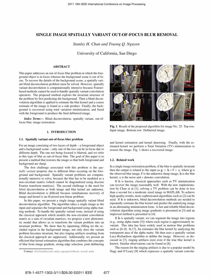
object boundary as shown in the left of Fig. 2.

To further understand the problem of the classical model, we

synthesize a blurred image using Eq. 2. The right of Fig. 2 is a

simulation of Eq. 2 in an extreme situation where hF is a delta func-

tion and hB is a “disk” function with large radius. Unwanted color

bleeding is observed around the object boundary, which is wrong be-

cause the foreground color should not contribute to the background

blur. The background color should be sky blue in the circled region.

Fig. 2: Insufficiency of Eq. 1. Left: Result of spatially variant TV

minimization [1]. Right: Simulation of Eq. 2 with hF being a delta

function and hB being a “disk” function with large radius.

2.2. Proposed Model

The proposed model follows from the work by Asada et al [10], and

has been previously used in [11,12]. In [10], the authors show that if

the foreground is in focus while the background is out of focus, the

observed foreground object boundary is a weighted average of the

background only. More precisely, suppose that the image f can be

written as f = αfF + (1− α)fB , where fF denotes the foreground

image and fB denotes the background image, the observed image

according to [10] should be

g = αfF + (1− α)(hB ∗ fB). (3)

The interpretation of Eq. 3 is that the observed image g is the com-

position of fF and hB ∗ fB . Note that the convolution of hB is

applied to the fB only, and is independent of fF .

The new model implies that if we can predict the occluded area

in hB ∗ fB (since a large area of hB ∗ fB is occluded by fF ), re-

covering the entire image f can be achieved by first recovering fBfrom hB ∗ fB and then fusing fB with fF (fF = αg can be pre-

determined using g and α). Note that recovering fB from hB ∗ fB is

spatially invariant. In other words we have transformed a spatially

variant problem to a spatially invariant problem, which is evidently

more efficient to solve than the brute force minimization [12].

3. PROPOSED ALGORITHM

The proposed algorithm consists of three key components: inpaint-

ing the background, kernel estimation and image restoration (see Al-

gorithm 1). Discussion on finding the alpha matte is skipped and we

refer to [5] for a thorough survey.

Algorithm 1 Proposed Algorithm

Input: g and α.Step 1: Inpainting background (Section 3.1)

gB = inpainting(g, α).Step 2: Kernel estimation (Section 3.2)

Initialize f = gB .

for i = 1 : m do

f̃ = shock filter(f).∇fs = edge selection(f̃).h̃ = argmin

h

‖∇fs ∗ h−∇gB‖2 + γ‖h‖2.

h = argminh

ν‖h− h̃‖2 + ‖h‖TV .

f = argminf

‖h ∗ f − gB‖2 + λ‖∇f −∇fs‖2.

end for

Step 3: Image restoration (Section 3.3)

fB = argminf

µ‖h ∗ f − gB‖2 + ‖f‖TV .

Output: f = αfF + (1− α)fB , where fF = αg.

3.1. Inpainting Background

Given a blurry observation g and the alpha matte α, the term g −αfF represents the observed background with foreground pixels re-

moved. The goal of the background inpainting step is to fill the

occluded pixels in g − αfF so that we can have an invariant decon-

volution procedure to recover fB .

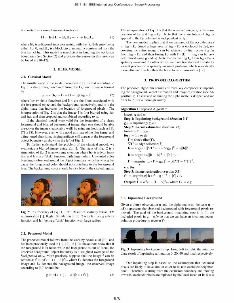
Fig. 3: Inpainting background step. From left to right: the interme-

diate result of inpainting at iteration 0, 20, 40 and final respectively.

Our inpainting step is based on the assumption that occluded

pixels are likely to have similar color to its non-occluded neighbor-

hood. Therefore, starting from the occlusion boundary and moving

inwards, occluded pixels are replaced by the local mean of its 5× 5

2011 18th IEEE International Conference on Image Processing

678

neighborhood. Fig. 3 illustrates a few iterations of the proposed in-

painting algorithm. Note that the algorithm works well around the

object boundary but works poorly in the central occluded region.

However, the poorly filled pixels in the central occluded region has

negligible effects to the deconvolution step as their geometric dis-

tance to the occlusion boundary is typically large. The filled back-

ground is denoted by gB .

3.2. Kernel Estimation

3.2.1. Shock Filter

As discussed in [3] and [4], salient edges are critical to blur kernel

estimation. To obtain salient edges, we follow [3] and apply Shock

filter to the observed image. Shock filtering is an iterative procedure

of which the k-th iteration is given by

fk+1 = f

k − β sign(∆fk)‖∇f

k‖1,

where initially f0 = hG ∗ fin, fin is the input to the shock filter (gB

in our case) and hG is a Gaussian blur kernel of size 9×9 and σ = 1.

∇f = [fx; fy] is the gradient of f and ∆f = f2x fxx+2fxfyfxy+f2y fyyis the Laplacian of f . β(= 1) is the step size. The shock filtered

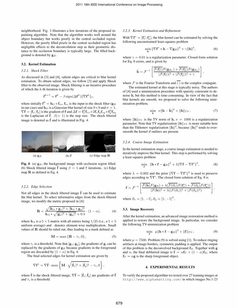
image is denoted as f̃ and is illustrated in Fig. 4.

(a) gB (b) f̃ (c) Edge map R

Fig. 4: (a) gB , the background image with occlusion region filled.

(b) Shock filtered image f̃ using β = 1 and 5 iterations. (c) Edge

map R as defined in Eq. 4.

3.2.2. Edge Selection

Not all edges in the shock filtered image f̃ can be used to estimate

the blur kernel. To select informative edges from the shock filtered

image, we modify the metric proposed in [4]:

R =

√

|hA ∗ gx|2 + |hA ∗ gy|2

hA ∗√

|gx|2 + |gy |2 + 0.5· (1− α), (4)

where hA is a 5× 5 matrix with all entries being 1/25 (i.e., a 5× 5uniform average) and · denotes element-wise multiplication. Small

values of R should be ruled out, thus leading to a mask defined as

M = max {R− τr, 0} , (5)

where τr is a threshold. Note that [gx; gy], the gradients of g, can be

replaced by the gradients of gB because gradients in the foreground

region are discarded by (1− α) in Eq. 4.

The final selected edges for kernel estimation are given by

∇fs = ∇f̃ ·max

{

M ·

√

|f̃x|2 + |f̃y |2 − τs, 0

}

,

where f̃ is the shock filtered image, ∇f̃ = [f̃x; f̃y] are gradients of f̃

and τs is a threshold.

3.2.3. Kernel Estimation and Refinement

With ∇fs = [fsx ; fsy ], the blur kernel can be estimated by solving the

following unconstrained least-squares problem

minh

‖∇fs ∗ h−∇gB‖2 + γ‖h‖2, (6)

where γ = 0.01 is a regularization parameter. Closed-form solution

for Eq. 6 exists, and is given by

h̃ = F−1

[

F(fsx)F(gBx) + F(fsy )F(gBy

)

|F(fsx)|2 + |F(fsy )|2 + γ

]

,

where F is the Fourier Transform and (·) is the complex conjugate.

The estimated kernel at this stage is typically noisy. The authors

of [4] used a minimization procedure with sparsity constraint to de-

noise h, but this method is time-consuming. In view of the fact that

blur kernels are smooth, we proposed to solve the following mini-

mization problem.

minh

ν‖h− h̃‖2 + ‖h‖TV , (7)

where ‖h‖TV is the TV norm of h, ν = 1000 is a regularization

parameter. Note that TV regularization ‖h‖TV is more suitable here

than the Tikhonov regularization ‖h‖2, because ‖h‖2 tends to over-

smooth the kernel if outliers are present.

3.2.4. Coarse Image Estimation

In the kernel estimation stage, a coarse image estimation is needed to

iteratively improve the blur kernel. This step is performed by solving

a least-squares problem

minf

‖h ∗ f − gB‖2 + λ‖∇f −∇fs‖2, (8)

where λ = 0.002 and the prior ‖∇f − ∇fs‖2 is used to preserve

edges according to ∇fs. The closed form solution of Eq. 8 is

f = F−1

[

F(h)F(gB) + λ(F(∂x)F(fsx) +F(∂y)F(fsy ))

|F(h)|2 + λ(|F(∂x)|2 + |F(∂y)|2)

]

,

where ∂x = [1, −1], ∂y = [1, −1]T .

3.3. Image Recovery

After the kernel estimation, an advanced image restoration method is

applied to restore the background image. In particular, we consider

the following TV-minimization problem

minf

µ‖h ∗ f − gB‖2 + ‖f‖TV , (9)

where µ = 7500. Problem (9) is solved using [1]. To reduce ringing

artifacts at image borders, symmetric padding is applied. The output

of this problem is the deconvolved background fB . Together with g

and α, the final deblurred image is f = αfF + (1 − α)fB, where

fF = αg is the sharp foreground object.

4. EXPERIMENTAL RESULTS

To verify the proposed algorithm we tested over 27 training images at

http://www.alphamatting.com/ in which images No.1-23

2011 18th IEEE International Conference on Image Processing

679

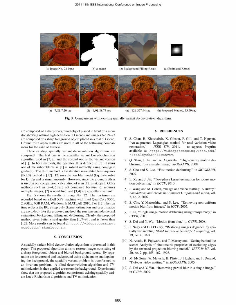
(a) Image No. 22 Input (b) α-matte (c) Background Filling Result (d) Estimated Kernel

(e) [7, 8], 7.20 sec (f) [1, 9], 88.73 sec (g) [12], 377.94 sec (h) Proposed Method, 33.79 sec

Fig. 5: Comparisons with existing spatially variant deconvolution algorithms.

are composed of a sharp foreground object placed in front of a mon-

itor showing natural high definition 3D scenes and images No.24-27

are composed of a sharp foreground object placed in a real 3D scene.

Ground truth alpha mattes are used in all of the following compar-

isons for the sake of fairness.

Three existing spatially variant deconvolution algorithms are

compared. The first one is the spatially variant Lucy-Richardson

algorithm used in [7, 8], and the second one is the variant version

of [1]. In both methods, the operator H is defined in Eq. 1 (thus

one of the subproblems in [1] is solved inexactly using conjugate

gradient). The third method is the iterative reweighted least-squares

(IRLS) method in [12]. [12] uses the new blur model (Eq. 3) to solve

for fF , fB and α simultaneously. However, since the ground truth αis used in our comparison, calculation of α in [12] is skipped. Other

methods such as [2–4, 6] are not compared because [6] requires

multiple images, [2] is non-blind, and [3, 4] are spatially invariant.

Fig. 5 shows the results of image No. 22. The run times are

recorded based on a Dell XPS machine with Intel Qual Core 9550,

2.8GHz, 4GB RAM, Windows 7/ MATLAB 2010. For [12], the run

time reflects the IRLS step only (kernel estimation and α estimation

are excluded). For the proposed method, the run time includes kernel

estimation, background filling and deblurring. Clearly, the proposed

method gives better visual quality than [1, 7–9] , and is faster than

[12]. More results can be found at http://videprocessing.

ucsd.edu/˜stanleychan.

5. CONCLUSION

A spatially variant blind deconvolution algorithm is presented in this

paper. The proposed algorithm aims to restore images consisting of

a sharp foreground object and blurred background scene. By sepa-

rating the foreground and background using alpha matte and inpaint-

ing the background, the spatially variant problem is transformed to

an invariant problem. A blind deconvolution algorithm and TV-

minimization is then applied to restore the background. Experiments

show that the proposed algorithm outperforms existing spatially vari-

ant Lucy-Richardson algorithms and TV minimization.

6. REFERENCES

[1] S. Chan, R. Khoshabeh, K. Gibson, P. Gill, and T. Nguyen,

“An augmented Lagrangian method for total variation video

restoration,” IEEE TIP, 2011, to appear. Preprint

available at http://videoprocessing.ucsd.edu/

˜stanleychan/deconvtv.

[2] Q. Shan, J. Jia, and A. Agarwala, “High-quality motion de-

blurring from a single image,” SIGGRAPH, 2008.

[3] S. Cho and S. Lee, “Fast motion deblurring,” in SIGGRAPH,

2009.

[4] L. Xu and J. Jia, “Two-phase kernel estimation for robust mo-

tion deblurring,” in ECCV, 2010.

[5] J. Wang and M. Cohen, “Image and video matting: A survey,”

Foundations and Trends in Computer Graphics and Vision, vol.

3, no. 2, 2007.

[6] S. Cho, Y. Matsushita, and S. Lee, “Removing non-uniform

motion blur from images,” in ICCV, 2007.

[7] J. Jia, “Single image motion deblurring using transparency,” in

CVPR, 2007.

[8] S. Dai and Y. Wu, “Motion from blur,” in CVPR, 2008.

[9] J. Nagy and D. O’Leary, “Restoring images degraded by spa-

tially variant blur,” SIAM Journal on Scientific Computing, vol.

19, no. 4, 1998.

[10] N. Asada, H. Fujiwara, and T. Matsuyama, “Seeing behind the

scene: Analysis of photometric properties of occluding edges

by the reversed projection blurring model,” IEEE PAMI, vol.

20, no. 2, pp. 155–167, 1998.

[11] M. McGuire, W. Matusik, H. Pfister, J. Hughes, and F. Durand,

“Defocus video matting,” in SIGGRAPH, 2005.

[12] S. Dai and Y. Wu, “Removing partial blur in a single image,”

in CVPR, 2009.

2011 18th IEEE International Conference on Image Processing

680