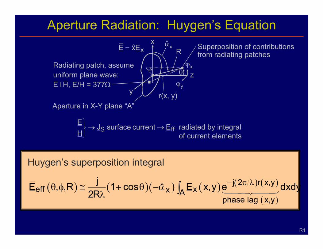
Aperture Radiation: Huygen’s Equation

y

zϕx

θ

Rx αx

r(x, y)

Superposition of contributions from radiating patches

ϕy

Aperture in X-Y plane “A”

Radiating patch, assumeuniform plane wave:E⊥H, E/H = 377Ω

ˆxExE =

( ) ( )( ) ( ) ( ) ( )

( )

− π λθ φ ≅ + θ −αλ ∫ j 2 r x,y

eff xx Aphase lag x,y

jE , ,R 1 cos E x,y e dxdyˆ2R

Huygen’s superposition integral

ffS E current surface JHE

→→⎭⎬⎫

radiated by integral of current elements

R1

Huygen’s Equation: Geometric approximations

2-D casex r(x) R

x sin ϕx0

ϕx

Aperture in x-y plane

x

( ) yxyxyx yxRsinysinxRyx,r :1, For ϕ−ϕ−≅ϕ−ϕ−≅<<ϕϕ

( ) ( ) ( )( )

∫ϕ+ϕ

λπ

+λπ

•αθ+λ

≅φθ A

yx2jx

K

x

R2j-

dxdyey,xEˆcos1R2

e jR,,E Thusyx

R2

( ) ( )( ) ( ) ( ) ( )

( )∫ πλ−α−θ+

λ≅φθ A

yx, lag phase

y,xr2jxxeff dxdyey,xEˆcos1

R2jR,,E

z

Huygen’s Equation: Geometric approximations

( )( ) ( )( )

( )( ) ( ) ( )∫ ϕϕϕϕ≅

∫≅ϕϕ

π

ϕ+ϕλπ

−−

ϕ+ϕλπ

+−

2 yxyx2j

yxx1

x

Ayx2j

x1

yx

dde,EKxvmy,xEx

dxdyey,xEKvm,E

yx

yx

R3

( ) ( ) ( )( )

∫ϕ+ϕ

λπ

+λπ

•αθ+λ

≅φθ A

yx2jx

K

x

R2j-

dxdyey,xEˆcos1R2

e jR,,E Thusyx

Huygen’s Equation: Geometric approximations

( )( ) ( ) ( )

( )( ) ( ) ( )∫ ϕϕϕϕ

λ≅

∫λ≅ϕϕ

πϕ+ϕπ−−

λλ

λλϕ+ϕπ+

λλ−

λλ

λλ

2 yxyx2j

yxx2

1

Ayx2j

x21

yx

dde,EK

xvmy,xEx

dydxey,xEKvm,E

yx

yx

R4

This is a Fourier transform pair

( ) ( ) ( ) ( )[ ]∫∫ π+π− == dfefXt x; dtetxfX Recall ft2jft2j

2cos1 , y y, x xLet ≅θ+λ

=λ

∆λλ

( )( ) ( )( )

( )( ) ( ) ( )∫

∫

π

ϕ+ϕλπ

−−

ϕ+ϕλπ

+−

ϕϕϕϕ≅

≅ϕϕ

2 yxyx2j

yxx1

x

A

yx2jx

1yx

dde,EKxvmy,xEx

dxdyey,xEKvm,E

yx

yx

Fourier Transform Relations

R5

Thus Aperture (pulse signal)

( )[ ] ( ) [ ]

( ) ( ) [ ]2-

o

2yxx

yx

21-2yxx

21-E

m W 2

,E,S

R at Vm ,E~Vm ,R yxx

η

ϕϕ=ϕϕ∝

ϕϕ↔ττ

↓↓

λλ

( )1Vm)y,x(E − ↔~ ( )[ ] R at Vm ,E 1yxx

−ϕϕ

Directivity D(θ, φ) of an Aperture AntennaLet P = radiation intensity andPTR = total power radiated (W) ( ) ( )

]m W[]m W[

R4PRf,,,P ,D 2-

2-

2TR π

φθ∆φθ

( )1, yx <<ϕϕ

R6

( )( )

( )( )

( )∫

∫

πη

λη

θ+≅

ϕ+ϕλπ

A22

xo

2

A

yx2jx

2o

2

R4dy dxy,xE2

1

dy dxey,xE

R22cos1D

yx

( ) ( )( )

( )∫

∫ϕ+ϕ

λπ

λ

θ+π=

A2

x

2

A

yx2jx

2

2

dy dxy,xE

dy dxey,xE cos1D

yx

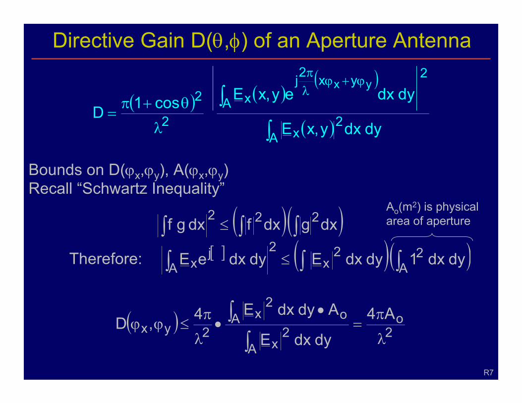
Directive Gain D(θ,φ) of an Aperture Antenna

Bounds on D(ϕx,ϕy), A(ϕx,ϕy)Recall “Schwartz Inequality”

( )( )∫∫∫ ≤ dxg dxfdx g f 222

( ) 2o

A2

x

A o2

x2yx

A4dydx E

Adydx E4,Dλ

π=

••

λ

π≤ϕϕ

∫∫

Therefore: [ ] ( )( )∫∫∫ ≤ A22

x2

Aj

x dydx 1 dydx Edydx eE

Ao(m2) is physical area of aperture

R7

( ) ( )( )

( )∫

∫ϕ+ϕ

λπ

λ

θ+π=

A2

x

2

A

yx2jx

2

2

dy dxy,xE

dy dxey,xE cos1D

yx

Directive Gain D(θ, φ) of an Aperture Antenna

( ) 2o

A2

x

A o2

x2yx

A4dydx E

Adydx E4,Dλ

π=

••

λ

π≤ϕϕ

∫∫

( )⇒

η

ϕϕ•

λ

π=

R

yxe2

,A4D But ( ) oyxe Aarea)(effective ,A Rη≤ϕϕ

where radiation efficiency 0.1R ≤η

= η •ηA Re oTherefore A A

Define “aperture efficiency” ηA

( ) 65.0A

maxA o

e

RA ≅

η∆η in practice; = 1 for uniform illumination

R8

Uniformly Illuminated Circular Aperture Antennas x

z

y r

φ’

φx

ϕyθ

Aperture coordinates = r, φ′Source coordinates = ϕx, ϕy for θ << 1

T1

( )( )

∫∫

φ

φ•

λ

θ+π=

ϕ+ϕλπ

A2

A

yx2j

2

2

'd dr rE

'd dr re1 cos1D

yx

0–3 dB

–17.6 dB–28.8 dB

0 1.63 4 7 10side lobes

πDλ

sin θ

P = 0

( ) ( )π πθ φ = + θ Λ θ

λ λ⎡ ⎤⎢ ⎥⎣ ⎦

221

D DD(f, , ) 1 cos sin

( )π= = π λ θ =

λ

22

oD

4 A at 0

q)q(J)q( 11 =Λ

“Lambda function”

where

“Bessel function of first kind”

Non-Uniformly Illuminated Circular Apertures

P θB1/2 θNULL #1 First Side - Lobe ηA

0 1.02 λ/D 1.22 λ/D 17.6 dB 1.001 1.27 λ/D 1.63 λ/D 24.6 dB 0.753 1.47 λ/D 2.93 λ/D 30.4 dB 0.56

Moretypical

G(θ)

θ

Ex(r)P = 0P = 1P = 2

0 D/2

( ) ( )= −⎡ ⎤⎢ ⎥⎣ ⎦

P2

x2r

Assume E r 1D

T2

Sidelobes and Backlobes of Aperture Antennas

Main lobe

Sidelobes Backlobes

Feed

Spillover

DiffractionBacklobes

Reflector

T3

Waveguide Horn Feeds

Pyramidal Horny D

Ey(y)

Ey(x)

⇒

DominantWaveguideMode TE10

⇒

0

Lower Sidelobes(∼25 dB)

G(ϕx)

Null at ϕ = λ/DG(ϕy)

High Sidelobes(∼17.6 dB)

φx

φy

T4

“Scalar” Feed

y

ApertureEy(y)

Yields very low sidelobes

λ/4 grooves cut into wall

Side view

∼λ/4 ⇒ open circuitat wall

λ/4 minimizesreturn echo

T5

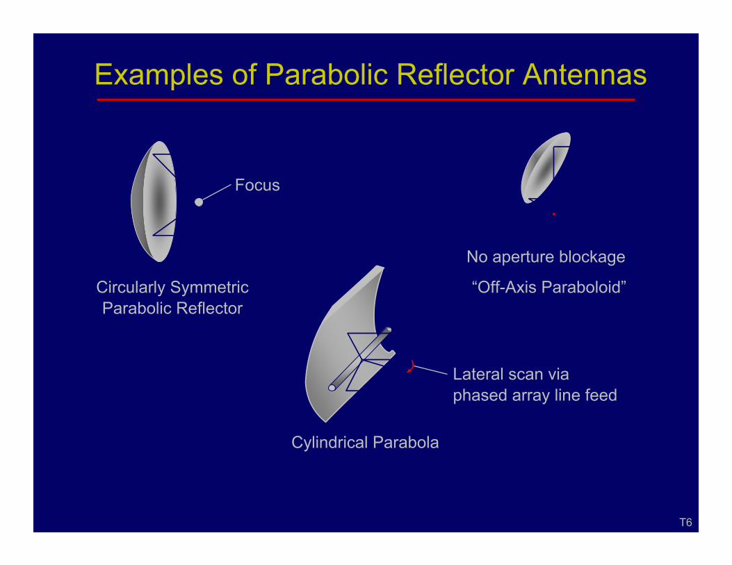
Examples of Parabolic Reflector Antennas

No aperture blockage

“Off-Axis Paraboloid”

Focus

Circularly SymmetricParabolic Reflector

T6

Lateral scan viaphased array line feed

Cylindrical Parabola

Spherical Reflector Antennas

Variable-pitchlinear phasedarray, positionedat line focus

Focus at ≥ R/2

Focal plane

R/2Center of curvature

T7

FeedSupport

BeamLine Feed

Illuminated Portione.g. Aricebo (1000’ = D, 600’ is illuminated)

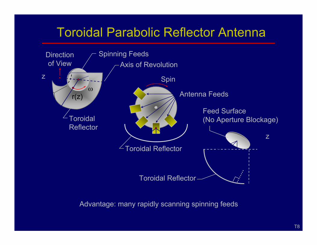
Toroidal Parabolic Reflector Antenna

ToroidalReflector

Directionof View

zAxis of Revolution

ω

Feed Surface(No Aperture Blockage)

r(z)

Spinning Feeds

Spin

Antenna Feeds

Toroidal Reflector

Advantage: many rapidly scanning spinning feeds

Toroidal Reflector

z

T8

Multifeed Arrays

ParabolaCB

Dx

y z

Focus “A”GA(θ)

GB(θ)

GC(θ)

θ

U1

f length Focal ∆=

sidelobes and G useable withbeams 5-3n ,5.0Df For o≅=

(say ~1 dB gain loss)

Can do much better with good lens systems

( ) direction- xin Df 2∝η

( ) 100055.07xn ,7Df if e.g. 2 ≅•≅=

“Scalar” Feed

y

ApertureEy(y)

Yields very low sidelobes

λ/4 grooves cut into wall

Side view

∼λ/4 ⇒ open circuitat wall

λ/4 minimizesreturn echo

U2

Multiple-Horn FeedsParabolicReflector

Adjacent Feeds

BA

Cross-over Pointbelow 3 dB, Far-Field

AB

Fourier Transform

Ey(y)Thus

Scalar Feeds

Cross-over ≤ 6 – 10 dBfor Low Sidelobes

Focal Plane

U3

Multiple-Horn Feeds

Feeds

1 2

3 4

Poor Coverage

Three-Array Solution

A B C AC A B C

A B C A B

Feed A′ is assembly ofexcited adjacent feeds

21

3 4

U4

Patterns

“Near-Field” Antenna Coupling

Near-field of aperture >> near field ofHertzian dipole (r << λ/2π)

Uniform Phase Front

SphericalPhase Front

r z

U5

DrD

≅•λ

λ≅

2Dr

λ>⇒

22D~r field" Far"

“Near-Field” Antenna Coupling

r << D2

λ

PT2PT1

Consider near-field link:Say: uniformly illuminated apertures

Ao

Eo(vm-1)

Ao/3

U62T

1r

1T

2r2T1r P

P

3

1

P

P i.e. ty)(reciproci

3

PP Claim ===

wattsA2

2EP o

o

o1T •

η=

3oA

2

2EP

o

o2T •

η=

,3

P

3oA

2

2EP 1T

o

o2r =•

η= ?P1r =

“Near-Field” Antenna Coupling, Mode Orthogonality

Only half the power is accepted here!Waves are not a sum of independent “bullets;” they have phase, modal structure (classic wave/particle issue).

U7

y y

Ey(y) Ey(y) receivedIlluminate only half

Eo

[ ]W 2

A

2

E o

o

2o •η

00

Halfgets in

Half reflected,orthogonal to dominant(coupled) mode

=+

( ) oo2

o 2A2E η

2Eo

2Eo