Sampling from distributive lattices – the Markov chain approach
63
Sampling from distributive lattices – the Markov chain approach Graduiertenkolleg MDS TU Berlin April 20., 2009 Stefan Felsner Technische Universit¨ at Berlin [email protected]
Transcript of Sampling from distributive lattices – the Markov chain approach

Sampling from distributive lattices –
the Markov chain approach
Graduiertenkolleg MDSTU BerlinApril 20., 2009
Stefan Felsner
Technische Universitat [email protected]

Topics
Markov Chain Monte Carlo
Coupling and CFTP
Distributive Lattices
α-Orientations and Heights
Block Coupling for Heights

The Sampling Problem
• Ω a (large) finite set
• µ : Ω→ [0, 1] a probability distribution
Problem. Sample from Ω according to µ.i.e., Pr(output = ω) = µ(ω).

The Sampling Problem
• Ω a (large) finite set
• µ : Ω→ [0, 1] a probability distribution
Problem. Sample from Ω according to µ.i.e., Pr(output = ω) = µ(ω).
There are many hard instances of the sampling problem.Relaxation: Approximate sampling
i.e., Pr(output = ω) = µ(ω) for some µ ≈ µ.
Applications of Sampling
• Get hand on typical examples from Ω.
• Approximate counting.

Preliminaries on Markov Chains
M transition matrix • size Ω×Ω
• entries ∈ [0, 1]
• row sums = 1 (stochastic)

Preliminaries on Markov Chains
M transition matrix • size Ω×Ω
• entries ∈ [0, 1]
• row sums = 1 (stochastic)
Intuition:
231413
23
14
13
012
0
M =
14
12
231
3
14
23
13
a
cb
M specifies a random walk

Instance of a Markov Chains
(X0, X1, X2, . . . Xr, . . .) an instance of M
• Xi random variable with values in Ω
• Pr(Xi+1 = x | Xi = s) = M(s, x)
Proposition.Probability distribution of Xt is µt with
µt = µ0 Mt
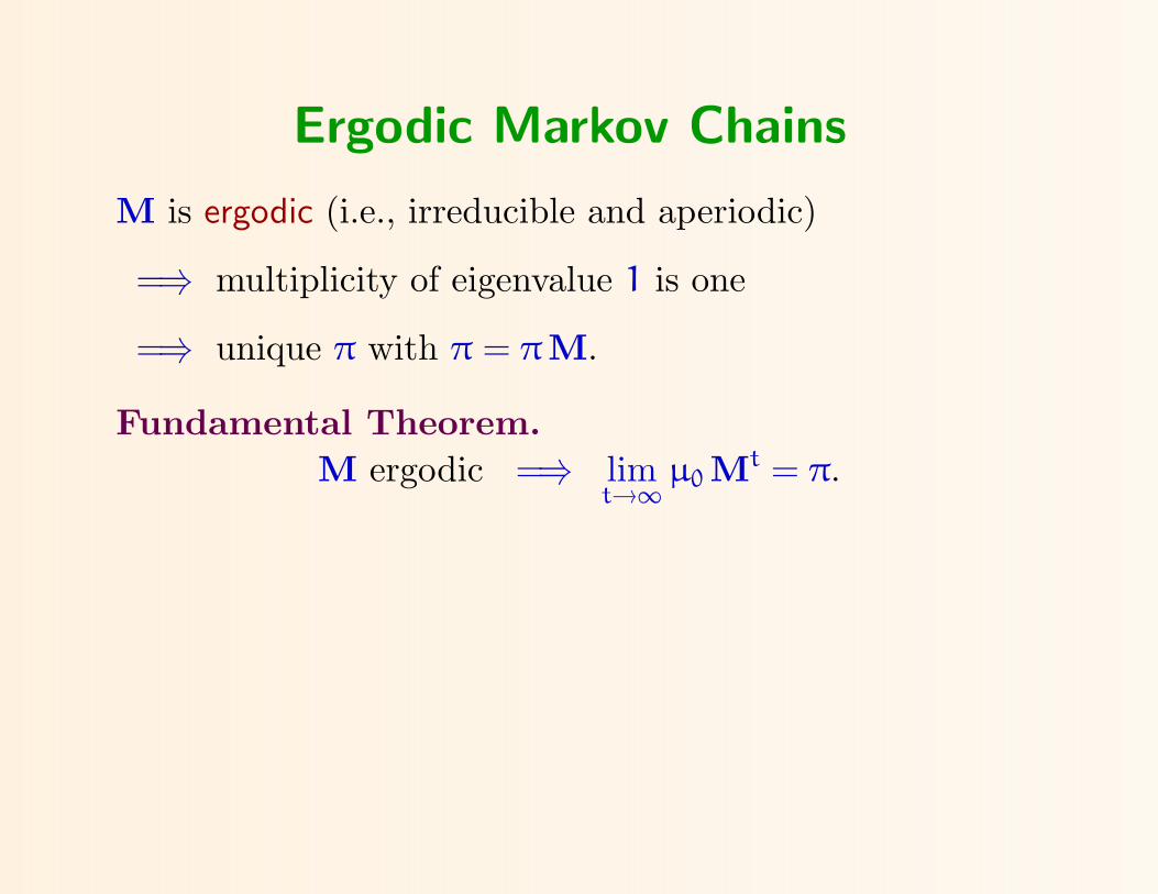
Ergodic Markov Chains
M is ergodic (i.e., irreducible and aperiodic)
=⇒ multiplicity of eigenvalue 1 is one
=⇒ unique π with π = πM.
Fundamental Theorem.M ergodic =⇒ lim
t→∞µ0 Mt = π.

Ergodic Markov Chains
M is ergodic (i.e., irreducible and aperiodic)
=⇒ multiplicity of eigenvalue 1 is one
=⇒ unique π with π = πM.
Fundamental Theorem.M ergodic =⇒ lim
t→∞µ0 Mt = π.
M symmetric and ergodic
=⇒ MT1
T = M1T = 1
T , hence 1M = 1
=⇒ π is the uniform distribution.
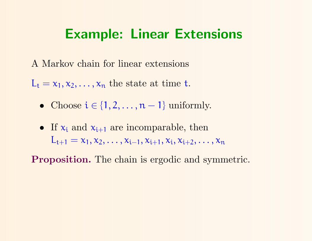
Example: Linear Extensions
A Markov chain for linear extensions
Lt = x1, x2, . . . , xn the state at time t.
• Choose i ∈ 1, 2, . . . , n − 1 uniformly.
• If xi and xi+1 are incomparable, thenLt+1 = x1, x2, . . . , xi−1, xi+1, xi, xi+2, . . . , xn
Proposition. The chain is ergodic and symmetric.
Measuring Convergence
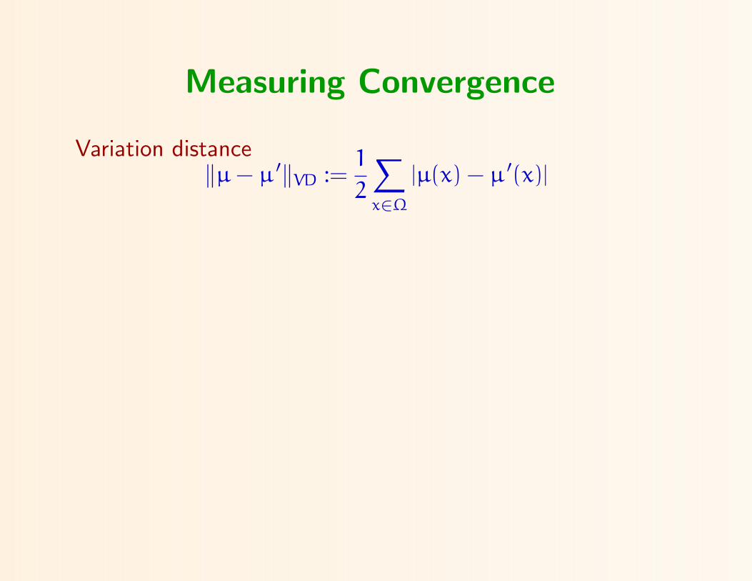
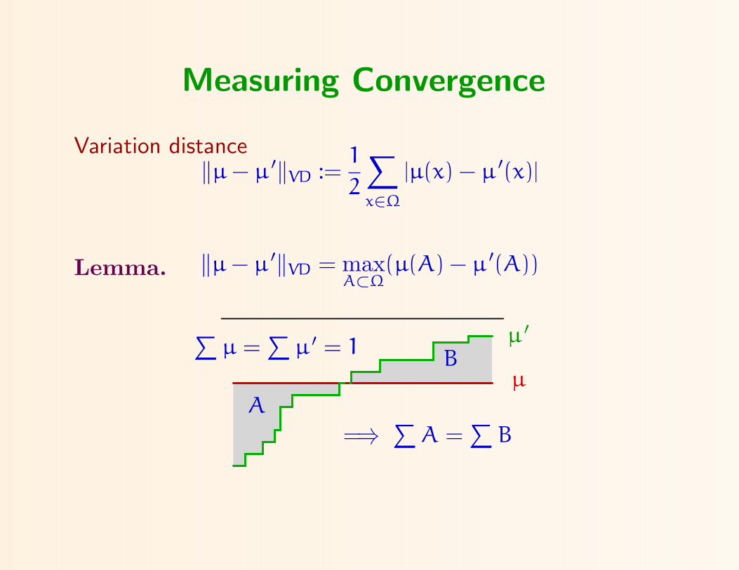
Variation distance‖µ − µ ′‖VD :=
1
2
∑x∈Ω
|µ(x) − µ ′(x)|
Measuring Convergence
Variation distance‖µ − µ ′‖VD :=
1
2
∑x∈Ω
|µ(x) − µ ′(x)|
Lemma. ‖µ − µ ′‖VD = maxA⊂Ω
(µ(A) − µ ′(A))
A
B
∑µ =∑
µ ′ = 1
=⇒ ∑A =
∑B
µ ′
µ

Mixing Time
µtx = δx Mt the distrib. after t steps starting in x
∆(t) := max( ‖µtx − π‖VD : x ∈ Ω)
τ(ε) = min( t : ∆(t) ≤ ε)
• τ(ε) is the mixing time.
• M is rapidly mixing ⇐⇒ τ(ε) is a polynomial functionof the problem size and log(ε−1).
Mixing Time and Eigenvalues
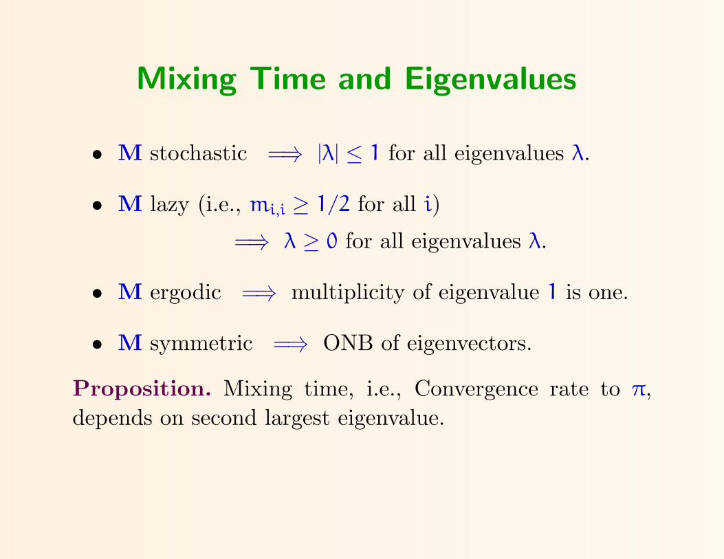
• M stochastic =⇒ |λ| ≤ 1 for all eigenvalues λ.
• M lazy (i.e., mi,i ≥ 1/2 for all i)
=⇒ λ ≥ 0 for all eigenvalues λ.
• M ergodic =⇒ multiplicity of eigenvalue 1 is one.
• M symmetric =⇒ ONB of eigenvectors.
Proposition. Mixing time, i.e., Convergence rate to π,depends on second largest eigenvalue.

Topics
Markov Chain Monte Carlo
Coupling and CFTP
Distributive Lattices
α-Orientations and Heights
Block Coupling for Heights
Coupling for Distributions
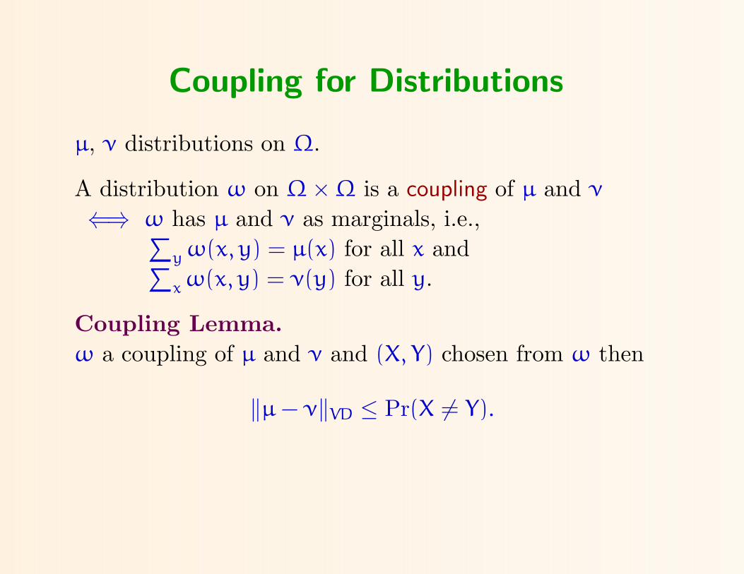
µ, ν distributions on Ω.
A distribution ω on Ω×Ω is a coupling of µ and ν⇐⇒ ω has µ and ν as marginals, i.e.,∑y ω(x, y) = µ(x) for all x and∑x ω(x, y) = ν(y) for all y.
Coupling Lemma.ω a coupling of µ and ν and (X, Y) chosen from ω then
‖µ − ν‖VD ≤ Pr(X 6= Y).
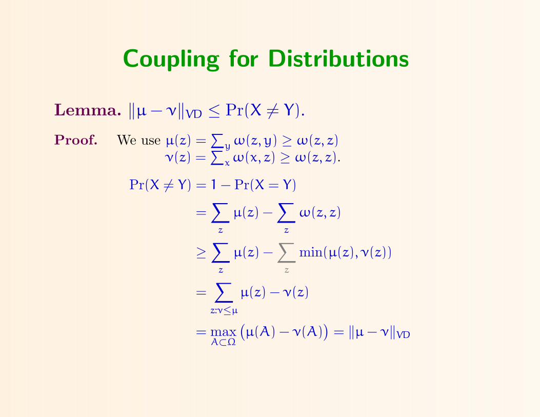
Coupling for Distributions
Lemma. ‖µ − ν‖VD ≤ Pr(X 6= Y).
Proof. We use µ(z) =∑
y ω(z, y) ≥ ω(z, z)ν(z) =
∑x ω(x, z) ≥ ω(z, z).
Pr(X 6= Y) = 1 − Pr(X = Y)
=∑
z
µ(z) −∑
z
ω(z, z)
≥∑
z
µ(z) −∑
z
min(µ(z), ν(z))
=∑
z:ν≤µ
µ(z) − ν(z)
= maxA⊂Ω
(µ(A) − ν(A)
)= ‖µ − ν‖VD
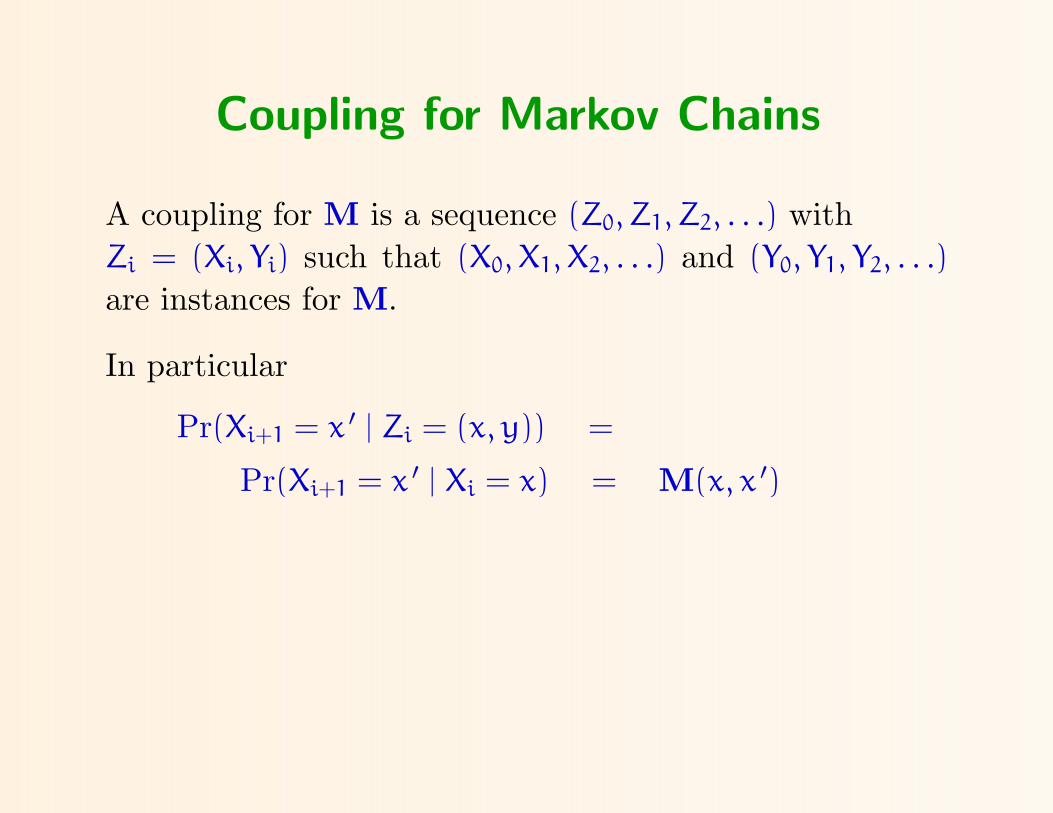
Coupling for Markov Chains
A coupling for M is a sequence (Z0, Z1, Z2, . . .) withZi = (Xi, Yi) such that (X0, X1, X2, . . .) and (Y0, Y1, Y2, . . .)
are instances for M.
In particular
Pr(Xi+1 = x ′ | Zi = (x, y)) =
Pr(Xi+1 = x ′ | Xi = x) = M(x, x ′)

Coupling and Mixing Times
Zi = (Xi, Yi) a coupling for M.
Theorem [Doblin 1938 ].If Pr
(XT 6= YT | Z0 = (x0, y0)
)< ε for every initial (x0, y0)
and T steps =⇒ τ(ε) ≤ T
Proof. Choose y0 from stationary distribution π
Yt is in stationary distribution π for all t
Xt is in distribution µtx0
.
Pr(XT 6= YT | Z0 = (x0, y0)
)< ε
Coupling Lemma =⇒ maxx ‖µTx − π‖VD < ε
definition of τ =⇒ τ(ε) ≤ T
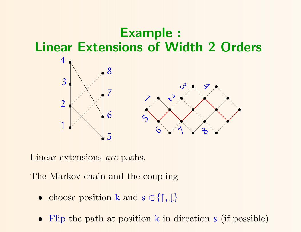
Example :Linear Extensions of Width 2 Orders
5
6
7
8
4
3
2
1
43
21
5
6 7 8
Linear extensions are paths.
The Markov chain and the coupling
• choose position k and s ∈ ↑, ↓• Flip the path at position k in direction s (if possible)
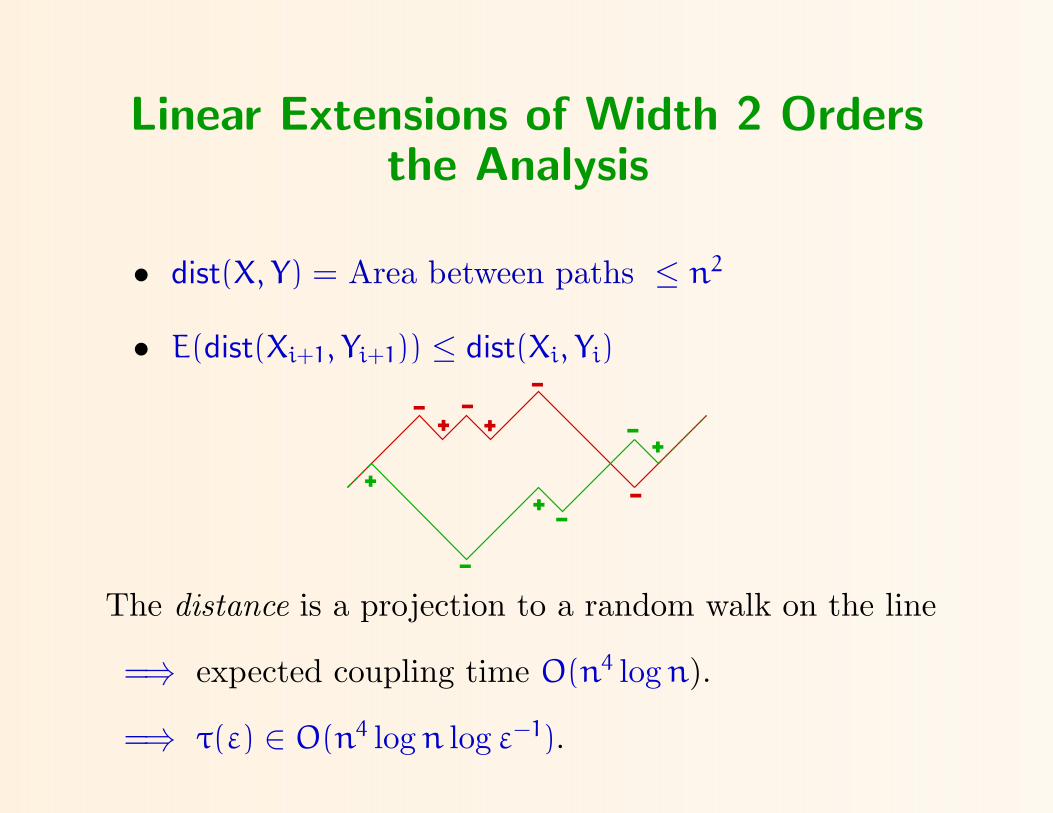
Linear Extensions of Width 2 Ordersthe Analysis
• dist(X, Y) = Area between paths ≤ n2
• E(dist(Xi+1, Yi+1)) ≤ dist(Xi, Yi)
The distance is a projection to a random walk on the line
=⇒ expected coupling time O(n4 log n).
=⇒ τ(ε) ∈ O(n4 log n log ε−1).
Coupling From the Past
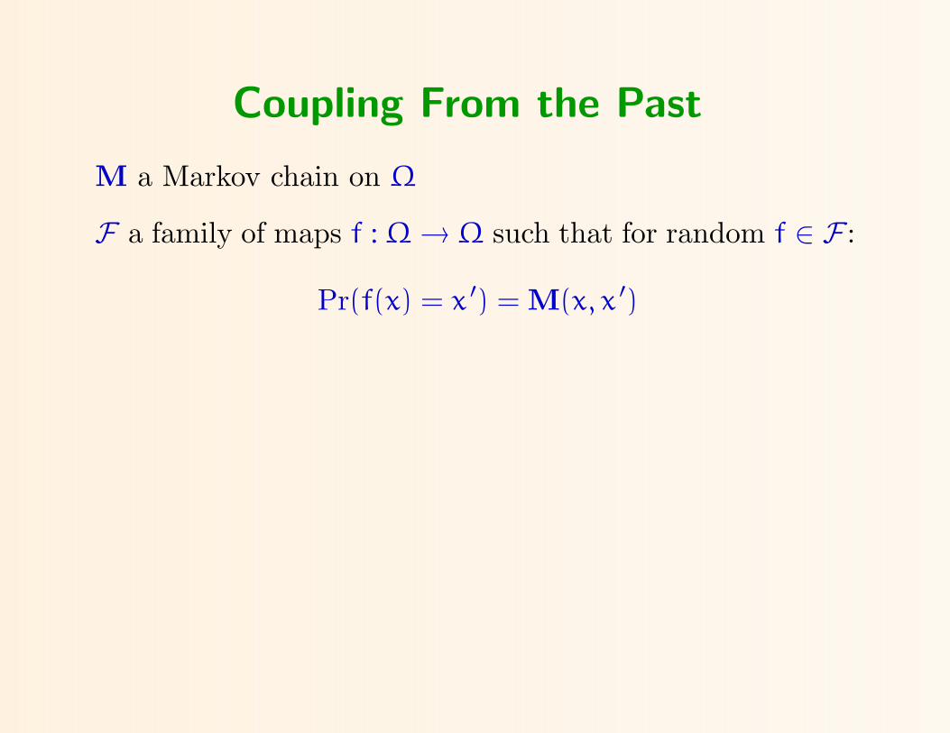
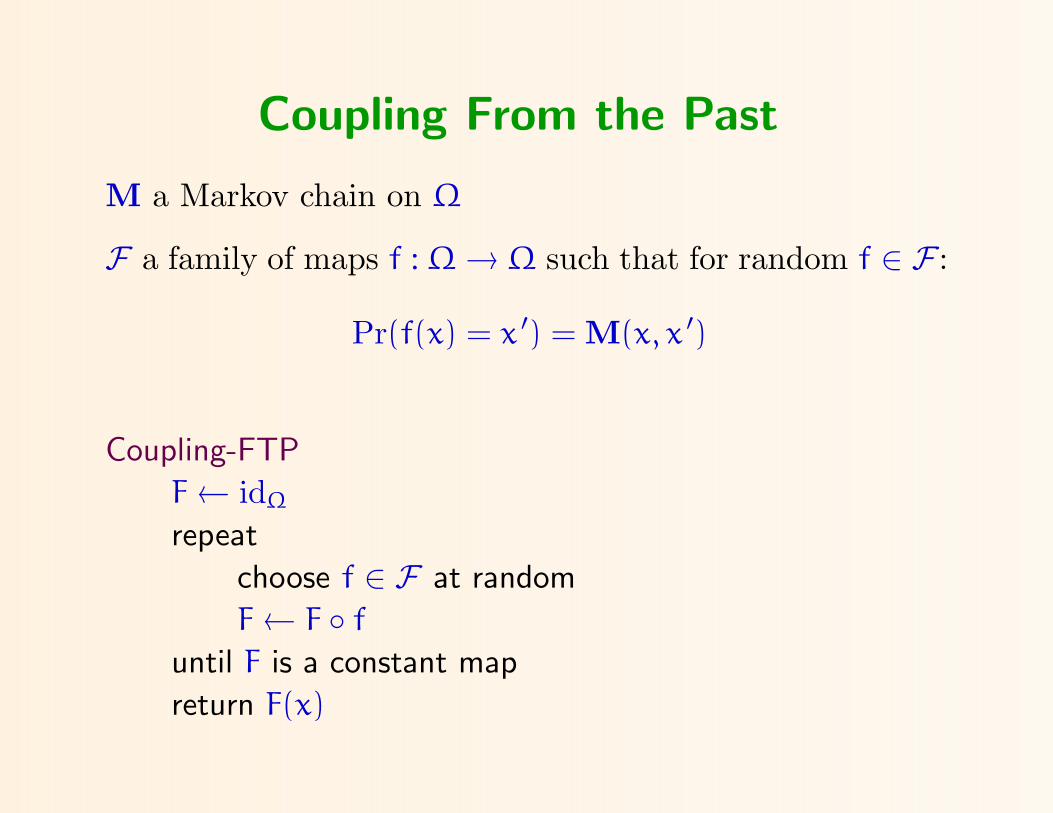
M a Markov chain on Ω
F a family of maps f : Ω→ Ω such that for random f ∈ F :
Pr(f(x) = x ′) = M(x, x ′)
Coupling From the Past
M a Markov chain on Ω
F a family of maps f : Ω→ Ω such that for random f ∈ F :
Pr(f(x) = x ′) = M(x, x ′)
Coupling-FTP
F← idΩ
repeat
choose f ∈ F at random
F← F f
until F is a constant map
return F(x)
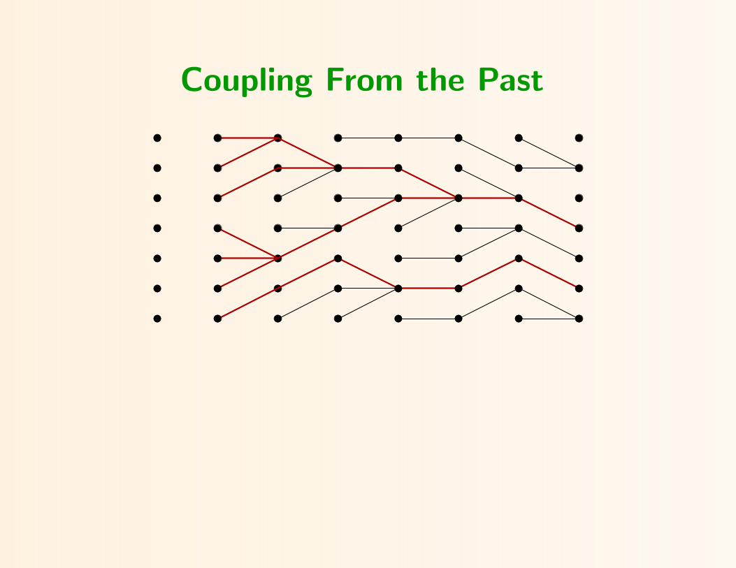
Coupling From the Past

Coupling From the Past
Theorem. The state returned by Coupling-FTP isexactly(!) in the stationary distribution.

Monotone Coupling From the Past:An Example
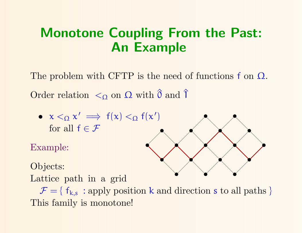
The problem with CFTP is the need of functions f on Ω.
Monotone Coupling From the Past:An Example
The problem with CFTP is the need of functions f on Ω.
Order relation <Ω on Ω with 0 and 1
• x <Ω x ′ =⇒ f(x) <Ω f(x ′)
for all f ∈ F
Example:
Objects:Lattice path in a gridF = fk,s : apply position k and direction s to all paths
This family is monotone!

Topics
Markov Chain Monte Carlo
Coupling and CFTP
Distributive Lattices
α-Orientations and Heights
Block Coupling for Heights

Distributive Lattices
Fact. L is a finite distributive lattice ⇐⇒there is a poset P such that that L is isomorphic to theinclusion order on downsets of P.
P
LP
654
1 2 3

Markov Chains on DistributiveLattices
A natural Markov chain on LP (lattice walk):
Identify state with downset D
• choose x ∈ P
choose s ∈ ↑, ↓• depending on s move to D + x or D − x
(if possible)
Fact. The chain is ergodic and symmetric,i.e, π is uniform.

Monotone Coupling on DistributiveLattices
The coupling family F :
fx,s: Use element x and direction s for all D.Is monotone!
=⇒ uniform sampling from distributive lattices is easy.

Monotone Coupling on DistributiveLattices
The coupling family F :
fx,s: Use element x and direction s for all D.Is monotone!
=⇒ uniform sampling from distributive lattices is easy.
Q: Is it fast (rapidly mixing)?
A: In most cases not.

Slow Mixing
• On distributive lattices based on Kleitman-Rothschildposets the mixing time of the lattice walk isexponential.
• The mixing time of the lattice walk is exponential forrandom bipartite graphs with degrees ≥ 6.(Dyer, Frieze and Jerrum)
Fast Mixing
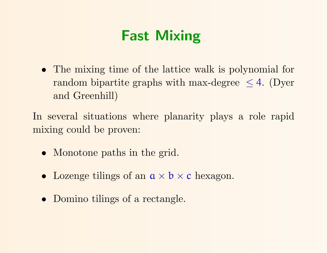
• The mixing time of the lattice walk is polynomial forrandom bipartite graphs with max-degree ≤ 4. (Dyerand Greenhill)
In several situations where planarity plays a role rapidmixing could be proven:
• Monotone paths in the grid.
• Lozenge tilings of an a× b× c hexagon.
• Domino tilings of a rectangle.
Topics
Markov Chain Monte Carlo
Coupling and CFTP
Distributive Lattices
α-Orientations and Heights
Block Coupling for Heights

alpha-Orientations
Definition. Given G = (V, E) and α : V → IN.An α-orientation of G is an orientation withoutdeg(v) = α(v) for all v.
Example.
Two orientations for the same α.

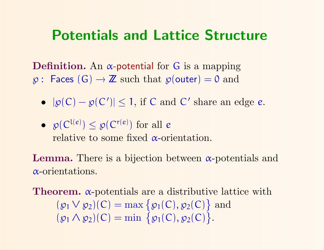
Potentials and Lattice Structure
Definition. An α-potential for G is a mapping℘ : Faces (G)→ ZZ such that ℘(outer) = 0 and
• |℘(C) − ℘(C ′)| ≤ 1, if C and C ′ share an edge e.
• ℘(Cl(e)) ≤ ℘(Cr(e)) for all e
relative to some fixed α-orientation.
Lemma. There is a bijection between α-potentials andα-orientations.
Theorem. α-potentials are a distributive lattice with(℘1 ∨ ℘2)(C) = max
℘1(C), ℘2(C)
and
(℘1 ∧ ℘2)(C) = min℘1(C), ℘2(C)
.

Counting and Sampling
Proposition. Counting α-orientations is #P-complete for
• planar maps with d(v) = 4 and α(v) ∈ 1, 2, 3 and
• planar maps with d(v) ∈ 3, 4, 5 and α(v) = 2.
Problem.
• Is counting 3-orientations in triangulations#P-complete?
• Is counting 2-orientations in quadrangulations#P-complete?
Approximate Counting
Fact. The fully polynomial randomized approximationscheme for counting perfect matchings of bipartite graphs(Jerrum, Sinclair and Vigoda 2001) can be used forapproximate counting of α-orientations.
Approximate Counting
Fact. The fully polynomial randomized approximationscheme for counting perfect matchings of bipartite graphs(Jerrum, Sinclair and Vigoda 2001) can be used forapproximate counting of α-orientations.
• What about the lattice walk?
Lattice Walks for alpha-Orientations
Theorem [Fehrenbach 03 ].• Sampling Eulerian orientations of simply connectedpatches of the quadrangular grid using the LW Markovchain is polynomial.
Theorem [Creed 05 ].• Sampling Eulerian orientations of simply connectedpatches of the triangular grid using the LW Markov chainis polynomial.
• Sampling Eulerian orientations of patches of thetriangular grid with holes using the LW Markov chain canbe exponential.

alpha-Orientations and Heights
G planar
Definition. An α-potential for G is a mapping℘ : Faces (G)→ ZZ such that ℘(outer) = 0 and
• |℘(C) − ℘(C ′)| ≤ 1, if C and C ′ share an edge e.
• ℘(Cl(e)) ≤ ℘(Cr(e)) for all e
relative to some fixed α-orientation.
Definition. A k-height for G is a mappingH : Faces (G)→ 0, ..., k such that
• |H(C) − H(C ′)| ≤ 1, if C and C ′ share an edge e.

Topics
Markov Chain Monte Carlo
Coupling and CFTP
Distributive Lattices
α-Orientations and Heights
Block Coupling for Heights

Height Lattices
Definition. A k-height for G is a mappingH : Faces (G)→ 0, ..., k such that
• |H(C) − H(C ′)| ≤ 1, if C and C ′ share an edge e.
Proposition. k-heights are a distributive lattice with
(H1 ∨ H2)(C) = maxH1(C), H2(C)
and
(H1 ∧ H2)(C) = minH1(C), H2(C)
.

Sampling from Height Lattices
We can use monotone CFTP to sample uniformly fromheight lattices.

Sampling from Height Lattices
We can use monotone CFTP to sample uniformly fromheight lattices.
A random 2-height on the 400× 400 square-grid.(38240593 steps)

Block Dynamics
• Experiments strongly suggest rapid mixingOur guess ckN
4 log(N).
• A rigorous proof of rapid mixing for 2-heights on torusgrids. We use block dynamics.

Block Dynamics
• Experiments strongly suggest rapid mixingOur guess ckN
4 log(N).
• A rigorous proof of rapid mixing for 2-heights on torusgrids. We use block dynamics.
Block dynamics:
• choose a block B ∈ B such that Pr(f ∈ B) = Pr(g ∈ B).
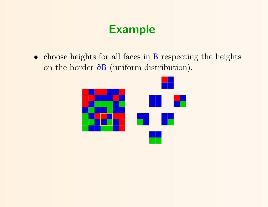
• choose heights for all faces in B respecting the heightson the border ∂B (uniform distribution).
Example
• choose heights for all faces in B respecting the heightson the border ∂B (uniform distribution).
Using Block Dynamics
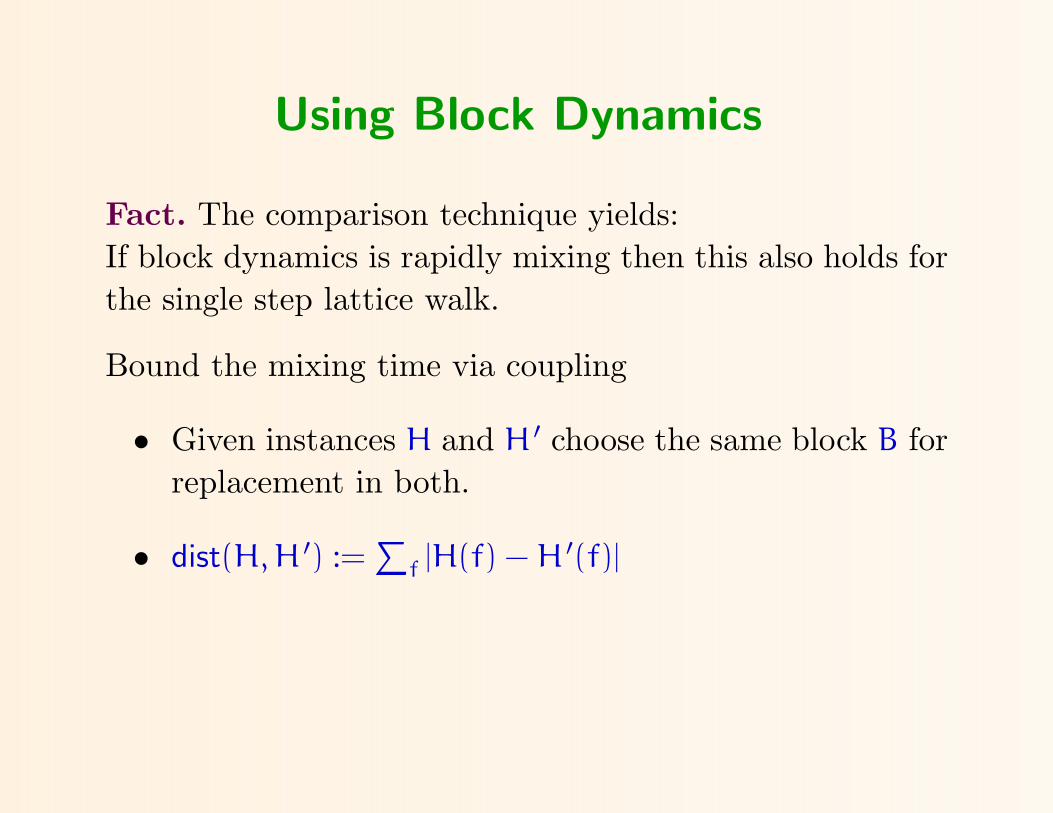
Fact. The comparison technique yields:If block dynamics is rapidly mixing then this also holds forthe single step lattice walk.
Bound the mixing time via coupling
• Given instances H and H ′ choose the same block B forreplacement in both.
• dist(H, H ′) :=∑
f |H(f) − H ′(f)|
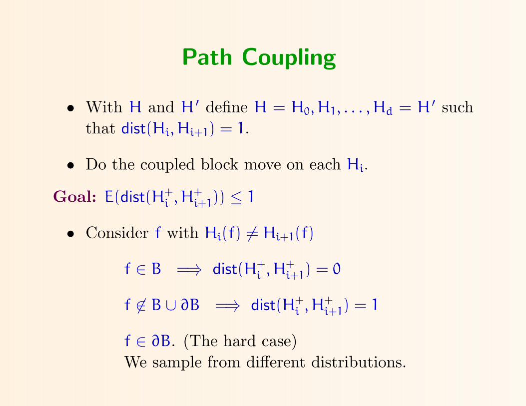
Path Coupling
• With H and H ′ define H = H0, H1, . . . , Hd = H ′ suchthat dist(Hi, Hi+1) = 1.
• Do the coupled block move on each Hi.
Goal: E(dist(H+i , H+
i+1)) ≤ 1
• Consider f with Hi(f) 6= Hi+1(f)
f ∈ B =⇒ dist(H+i , H+
i+1) = 0
f 6∈ B ∪ ∂B =⇒ dist(H+i , H+
i+1) = 1
f ∈ ∂B. (The hard case)We sample from different distributions.

The Hard Case
Set up a monotone coupling
Hi ≥ Hi+1 =⇒ H+i ≥ H+
i+1
(more about the existence later).
E(dist(H+i , H+
i+1)) = E(∑
f
|H+i (f) − H+
i+1(f)|)
= E(∑
f
H+i (f) − H+
i+1(f))
= E(∑
f
H+i (f)
)− E
(∑f
H+i+1(f)
)
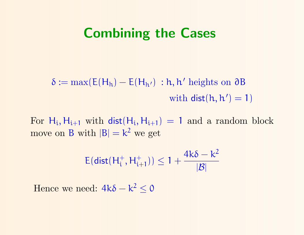
Combining the Cases
δ := max(E(Hh) − E(Hh ′) : h, h ′ heights on ∂B
with dist(h, h ′) = 1)
For Hi, Hi+1 with dist(Hi, Hi+1) = 1 and a random blockmove on B with |B| = k2 we get
E(dist(H+i , H+
i+1)) ≤ 1 +4kδ − k2
|B|
Hence we need: 4kδ − k2 ≤ 0
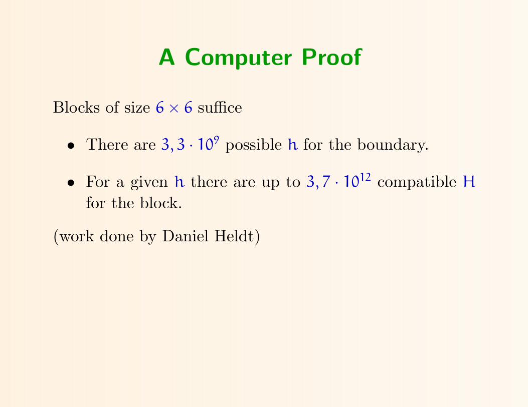
A Computer Proof
Blocks of size 6× 6 suffice
• There are 3, 3 · 109 possible h for the boundary.
• For a given h there are up to 3, 7 · 1012 compatible H
for the block.
(work done by Daniel Heldt)

Stochastic Dominance and Strassen’s
Definition. Stochastic dominance for distributions p1 andp2 on an ordered set (A,≤)
p1 ≤stoch p2 ⇐⇒ ∑a∈F
p1(a) ≤∑a∈F
p2(a) for all filter F ⊆ A
Theorem [Strassen ]. If p1 ≤stoch p2 on (A,≤) then thereis a distribution q on A×A with
• q(x, y) > 0 =⇒ x ≤ y
•∑
y q(x, y) = p1(x) and∑
x q(x, y) = p2(y)
(p1 and p2 are the marginals of q).
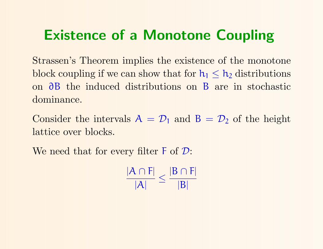
Existence of a Monotone Coupling
Strassen’s Theorem implies the existence of the monotoneblock coupling if we can show that for h1 ≤ h2 distributionson ∂B the induced distributions on B are in stochasticdominance.
Consider the intervals A = D1 and B = D2 of the heightlattice over blocks.
We need that for every filter F of D:
|A ∩ F|
|A|≤ |B ∩ F|
|B|

Existence of a Monotone Coupling
Goal: |A ∩ F||B| ≤ |B ∩ F||A|
Restrict attention to the lattice L spanned by min A andmax B. L is distributive, A is an ideal, B a filter of L.
Define f1 = χA∩F, f2 = χB, f3 = χB∩F and f4 = χA.
Lemma. f1(u)f2(v) ≤ f3(u ∨ v)f4(u ∧ v)
Ahlswede Daykin 4-Functions Theorem:
f1(U)f2(V) ≤ f3(U ∨ V)f4(U ∧ V)
We only need this for U = V = L.

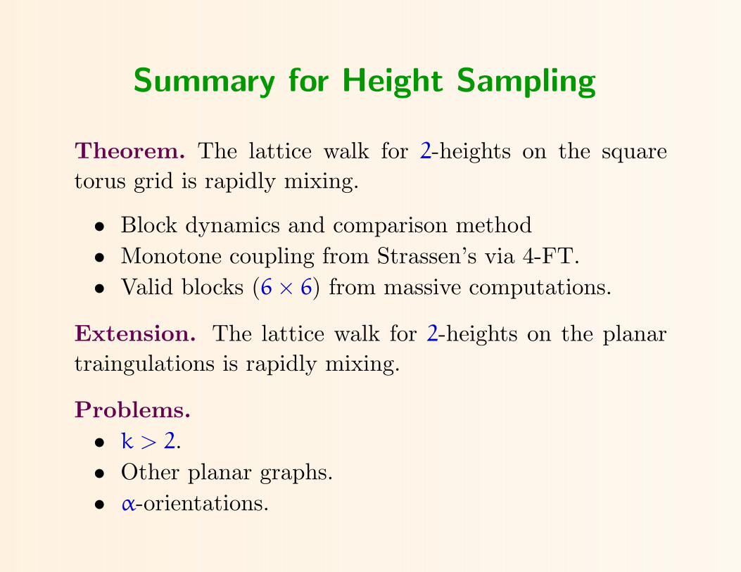
Summary for Height Sampling
Theorem. The lattice walk for 2-heights on the squaretorus grid is rapidly mixing.
• Block dynamics and comparison method• Monotone coupling from Strassen’s via 4-FT.• Valid blocks (6× 6) from massive computations.
Summary for Height Sampling
Theorem. The lattice walk for 2-heights on the squaretorus grid is rapidly mixing.
• Block dynamics and comparison method• Monotone coupling from Strassen’s via 4-FT.• Valid blocks (6× 6) from massive computations.
Extension. The lattice walk for 2-heights on the planartraingulations is rapidly mixing.
Problems.• k > 2.• Other planar graphs.• α-orientations.

The End
The End
Thank you.


![Magnon Hall effect and topology in kagome lattices: A ... · Magnon Hall effect and topology in kagome lattices: A theoretical investigation ... j (k)] 2. (11) | i (k) and. ε. i](https://static.fdocument.org/doc/165x107/5b02ce1d7f8b9a65618fcb88/magnon-hall-effect-and-topology-in-kagome-lattices-a-hall-effect-and-topology.jpg)