Distributive and Demand Cycles in the US Economy.pdf

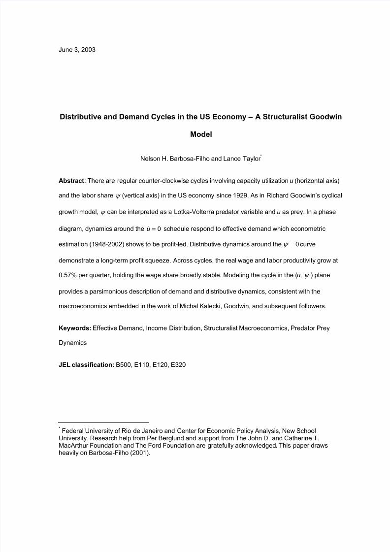
7/18/2019 Distributive and Demand Cycles in the US Economy.pdf

http://slidepdf.com/reader/full/distributive-and-demand-cycles-in-the-us-economypdf 1/23

June 3, 2003

Distributive and Demand Cycles in the US Economy – A Structuralist Goodwin

Model

Nelson H. Barbosa-Filho and Lance Taylor *

Abstract: There are regular counter-clockwise cycles involving capacity utilization u (horizontal axis)

and the labor share ψ (vertical axis) in the US economy since 1929. As in Richard Goodwin’s cyclical

growth model, ψ can be interpreted as a Lotka-Volterra predator variable and u as prey. In a phase

diagram, dynamics around the 0=u& schedule respond to effective demand which econometric

estimation (1948-2002) shows to be profit-led. Distributive dynamics around the 0=ψ & curve

demonstrate a long-term profit squeeze. Across cycles, the real wage and labor productivity grow at

0.57% per quarter, holding the wage share broadly stable. Modeling the cycle in the (u, ψ ) plane

provides a parsimonious description of demand and distributive dynamics, consistent with the

macroeconomics embedded in the work of Michal Kalecki, Goodwin, and subsequent followers.

Keywords: Effective Demand, Income Distribution, Structuralist Macroeconomics, Predator Prey

Dynamics

JEL classification: B500, E110, E120, E320

* Federal University of Rio de Janeiro and Center for Economic Policy Analysis, New SchoolUniversity. Research help from Per Berglund and support from The John D. and Catherine T.MacArthur Foundation and The Ford Foundation are gratefully acknowledged. This paper drawsheavily on Barbosa-Filho (2001).



2

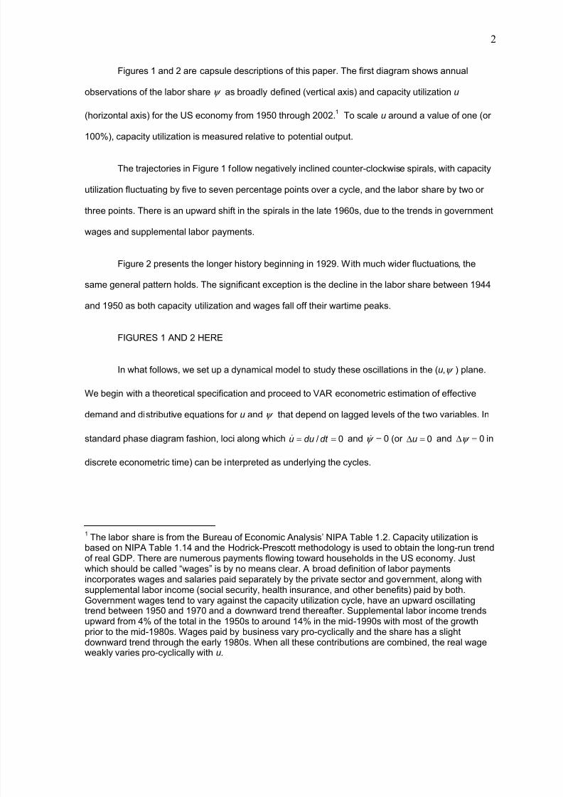
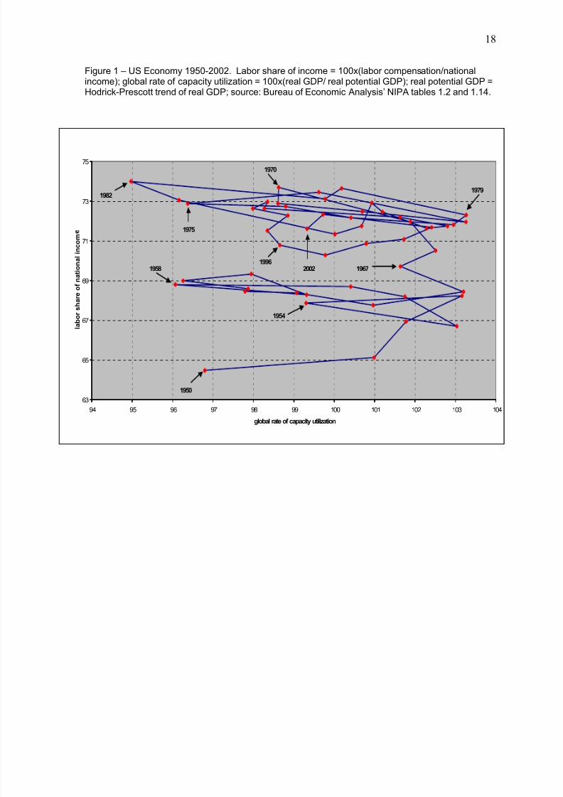
Figures 1 and 2 are capsule descriptions of this paper. The first diagram shows annual

observations of the labor share ψ as broadly defined (vertical axis) and capacity utilization u

(horizontal axis) for the US economy from 1950 through 2002.1 To scale u around a value of one (or

100%), capacity utilization is measured relative to potential output.

The trajectories in Figure 1 follow negatively inclined counter-clockwise spirals, with capacity

utilization fluctuating by five to seven percentage points over a cycle, and the labor share by two or

three points. There is an upward shift in the spirals in the late 1960s, due to the trends in government

wages and supplemental labor payments.

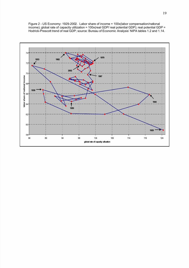
Figure 2 presents the longer history beginning in 1929. With much wider fluctuations, the

same general pattern holds. The significant exception is the decline in the labor share between 1944

and 1950 as both capacity utilization and wages fall off their wartime peaks.

FIGURES 1 AND 2 HERE

In what follows, we set up a dynamical model to study these oscillations in the (u,ψ ) plane.

We begin with a theoretical specification and proceed to VAR econometric estimation of effective

demand and distributive equations for u and ψ that depend on lagged levels of the two variables. In

standard phase diagram fashion, loci along which 0/ == dt duu& and 0=ψ & (or 0=∆u and 0=∆ψ in

discrete econometric time) can be interpreted as underlying the cycles.

1 The labor share is from the Bureau of Economic Analysis’ NIPA Table 1.2. Capacity utilization is

based on NIPA Table 1.14 and the Hodrick-Prescott methodology is used to obtain the long-run trend

of real GDP. There are numerous payments flowing toward households in the US economy. Justwhich should be called “wages” is by no means clear. A broad definition of labor paymentsincorporates wages and salaries paid separately by the private sector and government, along withsupplemental labor income (social security, health insurance, and other benefits) paid by both.Government wages tend to vary against the capacity utilization cycle, have an upward oscillatingtrend between 1950 and 1970 and a downward trend thereafter. Supplemental labor income trendsupward from 4% of the total in the 1950s to around 14% in the mid-1990s with most of the growthprior to the mid-1980s. Wages paid by business vary pro-cyclically and the share has a slightdownward trend through the early 1980s. When all these contributions are combined, the real wageweakly varies pro-cyclically with u.



3

1. Theory

Long ago, Richard Goodwin (1967) arbitraged mathematical models of species competition

from the 1920s (Lotka, 1925; Volterra, 1931) into economics, to set up a "predator-prey" scenario

involving distributive conflict between capitalists and workers. The workers, as it turns out, are the

predators with economic activity and employment as the prey. A whole econometric literature

followed in Goodwin's wake, e.g. Desai (1973), Gordon (1995), and Goldstein (1996). A general

finding is that “profit squeeze” cycles exist for the US economy. They are slightly damped and

therefore repetitive. These findings are replicated herein.

Along Marxist lines (Marglin, 1984), Goodwin assumed a fixed capital-output ratio and

savings-determined investment. Since he wrote, a body of structuralist theory dealing with demand

and distributive issues has emerged, inspired by the work of Michal Kalecki (1971). It bases the

determination of output on effective demand, and distributional dynamics upon social forces. There

are three major themes:

First, an effective demand curve exists in the (u,ψ ) plane. A positive slope implies that

demand is “wage-led,” reflecting the old left Keynesian idea that a powerful way to raise aggregate

spending is to engineer a shift in the functional income distribution toward labor (a strategy pursued

by Salvador Allende’s government in Chile in the early 1970s, for example). With a strong

accelerator response of investment to higher workers’ consumption, output expansion can be shown

to be a possible response to the distributional shift.

A negative slope signifies “profit-led” demand, which could result from higher investment

stimulated by a bigger profit share and/or more exports due to increased international

competitiveness resulting from lower unit labor costs (also indexed byψ ). Econometric evidence (for

example, Bowles and Boyer, 1995) suggests that demand in developed economies is profit-led.



4

Because devaluation cuts real wages and is often associated with output contraction in developing

economies, their effective demand may typically be wage-led.2

Second, as will be shown below, one can similarly derive a “distributive” curve giving a long-

term relationship between the wage share and capacity utilization. Its configuration depends on how

real wage and labor productivity growth interact over the cycle. If it has a positive slope, the schedule

along which 0=ψ & could be called “Marxist” or seen as demonstrating a profit squeeze in the sense

that the profit share would fall if the level of capacity utilization were to rise in the long run. Subject to

stability complications discussed below, a negative slope embodies “forced saving” and could be

called “Kaldorian.”3

Third, the effective demand and distributive curves can be combined to generate a model of

cyclical growth, precisely along Goodwin’s lines. Because by construction u and ψ vary in limited

ranges, they can underlie a pair of differential equations which are generally stationary and thereby

straightforward to analyze.

Details follow for one particular specification. We first look at overall capacity utilization as an

indicator of effective demand and then real wage and productivity dynamics on the side of

distribution. Subsequently we take up behavior of the nominal wage and price levels, and the

components of demand.

To model the output cycle as driven from the demand side, we treat capacity utilization u as a

continuously differentiable function of time. Let X stand for output and Q for capacity. Then Q X u /=

and logarithmic differentiation gives the relationship

2 The notions of wage- and profit-led demand trace to papers written independently by Rowthorn

(1982) and Dutt (1984), who in turn followed Kalecki’s colleague Josef Steindl (1952). Bhaduri andMarglin (1990) expand on their models and Blecker (2002) and Taylor (2003) provide recent literaturereviews.3 Forced saving involves a distributive shift toward profits to generate saving to finance higher

investment as effective demand rises in the long run. This mode of macro adjustment was proposedin the early 19

th century or even before, and Kaldor (1956, 1957) was its main post-WWII exponent.

Boddy and Crotty (1975) and Bowles, Gordon, and Weisskopf (1990) develop models of the USeconomy incorporating a profit squeeze.



5

Q X u ˆˆˆ −= (1)

with uuudt duu //)/(ˆ &== , etc. As will be seen, this specification readily generates cycles, and is

consistent with the relatively small changes quarter-by-quarter typically observed in macro time series

for aggregate demand and distribution.

Similarly, we have ξ ω ψ /= as the labor share, where P W /=ω is the real wage (with W

and P as the nominal wage and price level respectively) and L X /=ξ is labor productivity. The

analog to (1) is

ξ ω ψ ˆˆˆ −= . (2)

This equation shows that ψ is determined over time by the bargain affecting the nominal wage W,

pricing behavior by firms which sets P, and combined social and technological forces that impinge

upon labor productivity growth.

In growth rate form, the model can be restated in four equations based upon capacity

utilization and the labor share:

ψ α α α ψ ++= u X u0ˆ , (3)

ψ β β β ψ ++= uQ u0ˆ , (4)

ψ γ γ γ ω ψ ++= uu0ˆ , (5)

and

ψ δ δ δ ξ ψ ++= uu0ˆ . (6)

If we set i i i β α φ -= and i i i δ γ θ -= , then substituting (3)-(4) into (1) and (5)-(6) into (2) gives

reduced form equations for u and ψ :



6

)( 0 ψ φ φ φ ψ ++= uuu u& (7)

and

)( 0 ψ θ θ θ ψ ψ ψ ++= uu& . (8)

What can we say about the signs of the coefficients in (7) and (8)?

Beginning with equation (3), evidence presented below and elsewhere suggests that effective

demand in the US and other advanced countries is profit-led, so that 0<ψ α . There is a general

consensus that the basic Keynesian stability condition 0/ <∂∂ X X & is satisfied, or 0<uα . In (4), we

assume that capacity Q is largely determined by the existing capital stock. Capital formation usually

responds positively to both the level of economic activity and profitability, so that 0>u β and 0<ψ β .

It follows immediately that 0<uφ so 0/ <∂∂ uu& in (7) and the differential equation is locally stable in u.

Via the multiplier, the overall negative demand effect of a higher value of ψ should outweigh

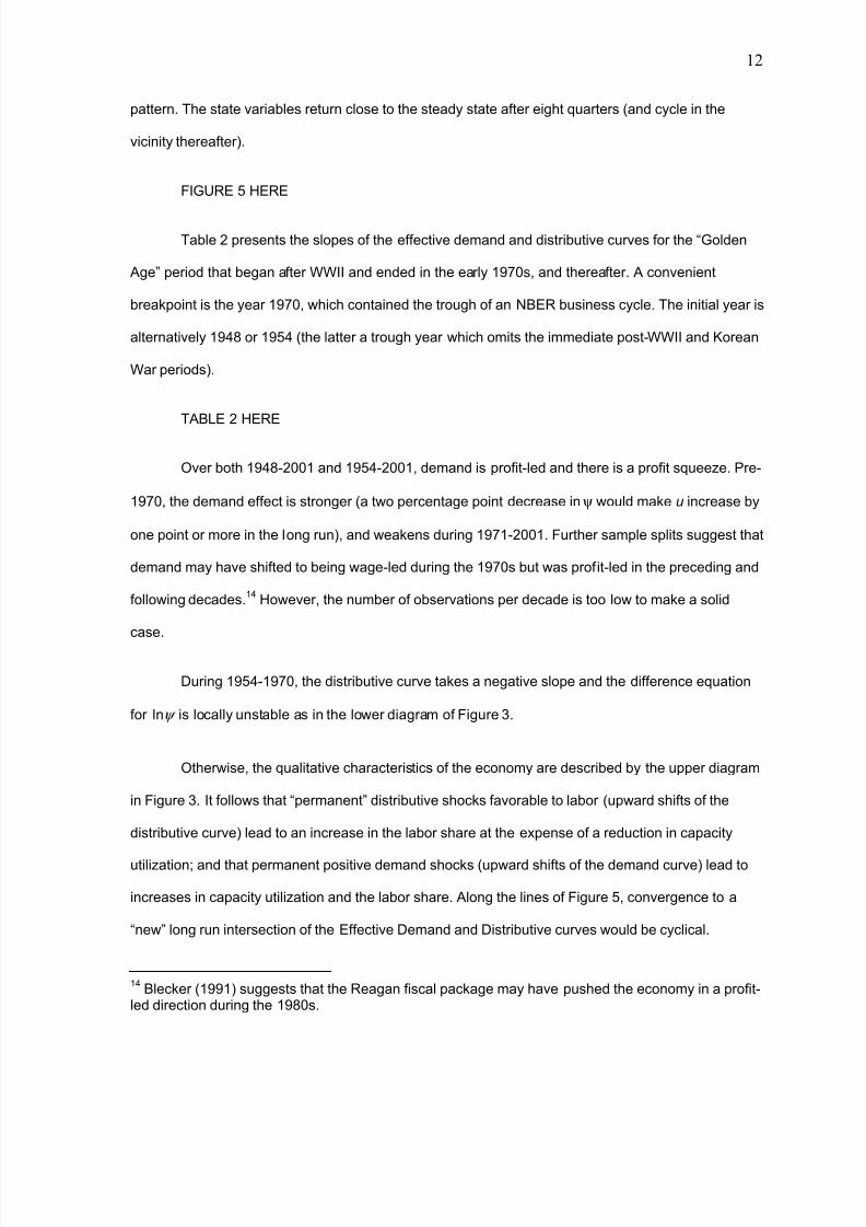
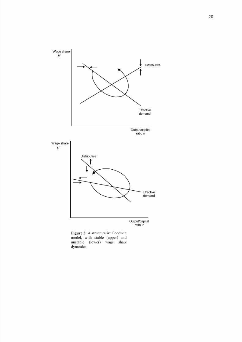
its specific effect on investment, ψ ψ β α > , so that 0<ψ φ . In both diagrams in Figure 3, the

"Effective demand" schedule along which 0=u& has a negative slope ψ φ φ ψ // udud −= in the (u,ψ )

plane. In the long run, a higher labor share is associated with lower capacity utilization.

FIGURE 3 HERE

The story about the "Distributive" curve along which 0=ψ & is tangled. In the US the real

wage rises in line with productivity across cycles, thereby holding ψ rather stable when it is averaged

over long periods. During the course of one cycle, Figures 1 and 2 suggest that ξ ω ψ /= rises when

u falls and vice versa. In other words, when u swings up productivity growth exceeds real wage

growth with the opposite occurring during a downswing in capacity utilization.

The econometric results reported below suggest that the (detrended) price level responds

positively to lagged levels of ψ as an indicator of unit labor cost and negatively to lagged u via a



7

mildly counter-cyclical aggregate mark-up. Both responses are weak so that P is relatively stable over

the cycle. In other words, shifts in the real wage ω are largely driven by the (again detrended) money

wage W . As it turns out, W responds positively to both state variables but more strongly to ψ than u.

so cyclical real wage dynamics are principally driven by money wage reactions to changes in the

labor share. The bargaining interpretation would be that at the macro level labor’s market power is

enhanced when the wage share is high.

Similar observations apply to labor productivity L X /=ξ . We know already from the

demand side of the model that X tends to fall when ψ increases. The econometric results below

suggest that ξ reacts positively to lagged values of both u and ψ . As with the real wage, the ψ -

effect is stronger. It can be positive only if L falls more than X when ψ rises. This pattern must be

interpreted along cyclical lines. During a downswing in u, ψ tends to increase. A positive lagged

response of ξ to ψ is then consistent with a rise in productivity during and after the cyclical trough –

the observed pattern.

The positive effects of both u and ψ on the real wage are stronger than those on productivity.

An immediate implication is that 0>−= uuu δ γ θ and 0/ <∂∂ uψ & , i.e. there is a short-run profit

squeeze. Translating the VAR econometric difference equation presented below into differential

equation language, it will also be true that 0/ <∂∂ ψ ψ & in (8); that equation is locally stable. However,

during the period 1955-70 the regression results suggest that 0<<ψ δ , with productivity growth

responding strongly to increases in the profit share and making 0>ψ θ so that 0/ >ψ ψ d d & as well.

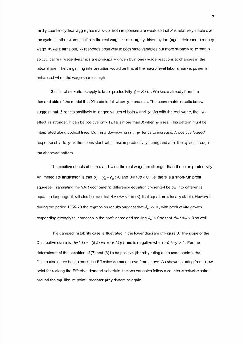
This damped instability case is illustrated in the lower diagram of Figure 3. The slope of the

Distributive curve is )//()/(/ ψ ψ ψ ψ ∂∂∂∂−= && udud and is negative when 0/ >∂∂ ψ ψ & . For the

determinant of the Jacobian of (7) and (8) to be positive (thereby ruling out a saddlepoint), the

Distributive curve has to cross the Effective demand curve from above. As shown, starting from a low

point for u along the Effective demand schedule, the two variables follow a counter-clockwise spiral

around the equilibrium point: predator-prey dynamics again.



8

The upper diagram corresponds to 0/ <∂∂ ψ ψ & . The Distributive curve slopes upward so that

there is a profit squeeze. The two-equation system is dynamically stable and can also demonstrate

cyclical behavior.4

Finally, although it does not appear to be empirically relevant in the US, a stable forced

saving/Kaldorian Distributive schedule would have 0/ <∂∂ ψ ψ & and .0/ <∂∂ uψ & The Distributive

curve would have a negative slope. A profit-led (negatively sloped) Effective demand schedule would

have to cut it from above for the overall system to be stable.

2. Evidence for the United States

To our knowledge, the model just sketched has not been estimated as a full system.5

Here

we present an initial attempt.

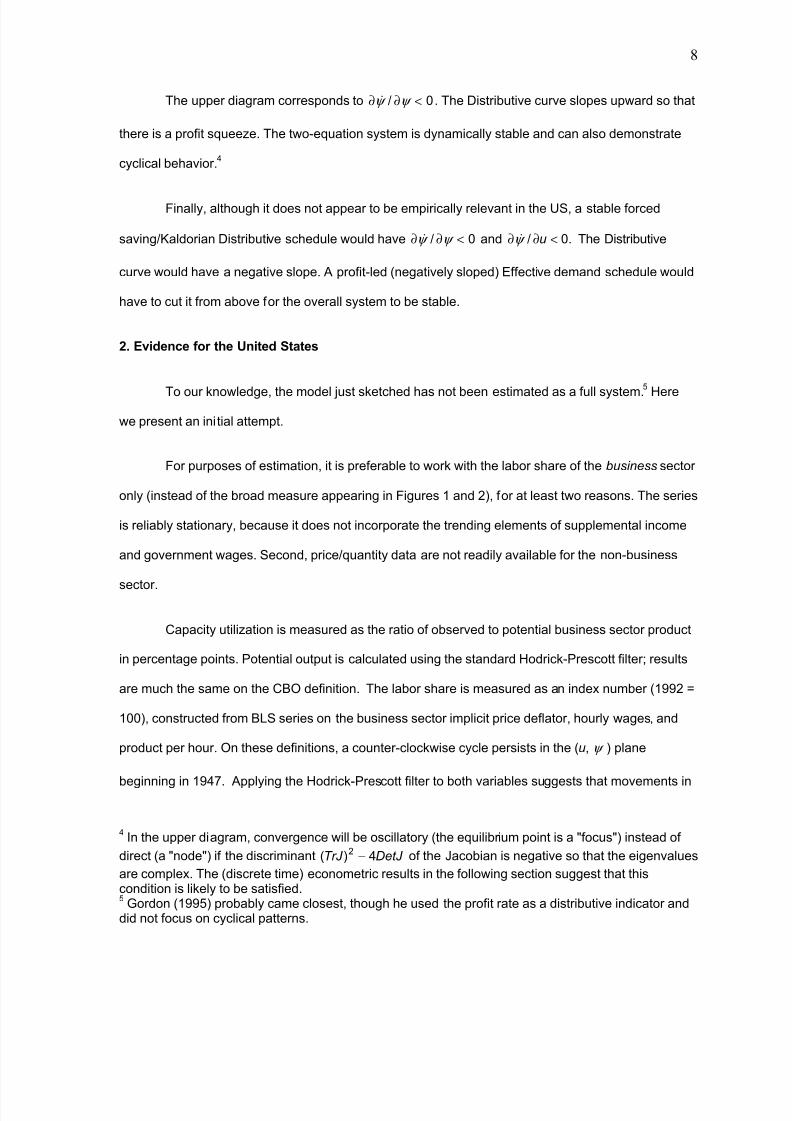
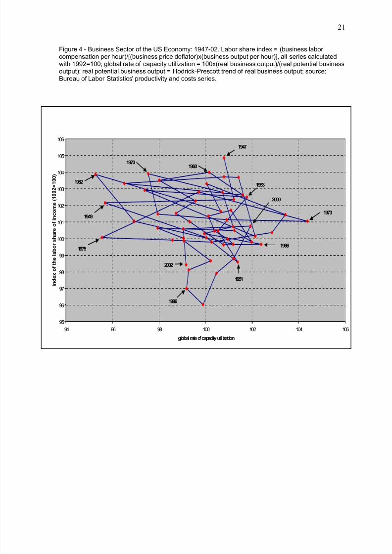
For purposes of estimation, it is preferable to work with the labor share of the business sector

only (instead of the broad measure appearing in Figures 1 and 2), for at least two reasons. The series

is reliably stationary, because it does not incorporate the trending elements of supplemental income

and government wages. Second, price/quantity data are not readily available for the non-business

sector.

Capacity utilization is measured as the ratio of observed to potential business sector product

in percentage points. Potential output is calculated using the standard Hodrick-Prescott filter; results

are much the same on the CBO definition. The labor share is measured as an index number (1992 =

100), constructed from BLS series on the business sector implicit price deflator, hourly wages, and

product per hour. On these definitions, a counter-clockwise cycle persists in the (u, ψ ) plane

beginning in 1947. Applying the Hodrick-Prescott filter to both variables suggests that movements in

4 In the upper diagram, convergence will be oscillatory (the equilibrium point is a "focus") instead of

direct (a "node") if the discriminant DetJ TrJ 4)( 2 − of the Jacobian is negative so that the eigenvalues

are complex. The (discrete time) econometric results in the following section suggest that thiscondition is likely to be satisfied.5 Gordon (1995) probably came closest, though he used the profit rate as a distributive indicator and

did not focus on cyclical patterns.



9

capacity utilization lead those of the labor share throughout most of the post-World War II period –

predator is led by prey.

FIGURE 4 HERE

For decomposition analysis,6 we can write t t t t t g ni c u +++= at time t, with the four demand

components being consumption t c , investment t i , net exports t n , and government spending t g

measured relative to potential GDP. Implicitly, potential GDP and potential business sector GDP are

assumed to correlate closely, which they do.

To impose a linear decomposition of ψ into its components, regression equations have to be

specified for ψ ln to obtain the determinants of the distributive curve. More precisely, define

ψ ψ ψ lnln)( −= t t f where t ψ is the wage share at time t and ψ is its sample mean. For sample

values close to the mean, we have

1)/())(/1()(lnln −=−+≈− ψ ψ ψ ψ ψ ψ ψ ψ t t t f .

This is an approximate linear relationship between ψ and ψ ln , which in turn decomposes as

ξ ψ lnlnlnln −−= P W , parallel to the additive breakdown of aggregate demand into its components

presented above.

Measured in index number form, variations in ψ slightly exceed those of u over cycles. Both

series are stationary at the 1% level of significance on Augmented Dickey-Fuller tests.7

To have the explanatory variables expressed in the same functional forms, the regression

equations were estimated for u and ψ to analyze the demand curve, and for uln and ψ ln to analyze

6 The appendix presents the methodology to decompose the aggregated VAR coefficients, estimated

for the dynamics of u and ψ , into their distributive and demand components. For a detailed

description, see Barbosa-Filho (2003).7 The ADF tests were done with zero to seven lagged differences and no trend in the estimated

equations for both variables. To have the same sample for all lag specifications, the tests were runfor the 1949-2002 sample. At 1% and 5% of statistical significance, respectively, the unit-root null isrejected for u and ψ in all lag specifications.



10

the distributive curve.8 In both cases the distributive-demand dynamics were studied using an off-the-

shelf vector autoregressive (VAR) model of the form

t εyΦηtµy

L

1 j jt jt

+++=

∑=−

where '][ t t t uψ =y in the “demand” VAR and ]ln[ln ′t t uψ in the “distributive” VAR, µ , η and j Φ ,

are coefficient matrices of appropriate dimensions and, by construction, t ε is vector of white-noise

disturbances.9

To define the lag structure of the model, we set eight as the maximum length and computed

Akaike and Schwarz information criteria for all specifications. The results indicated that two is the best

lag length.10

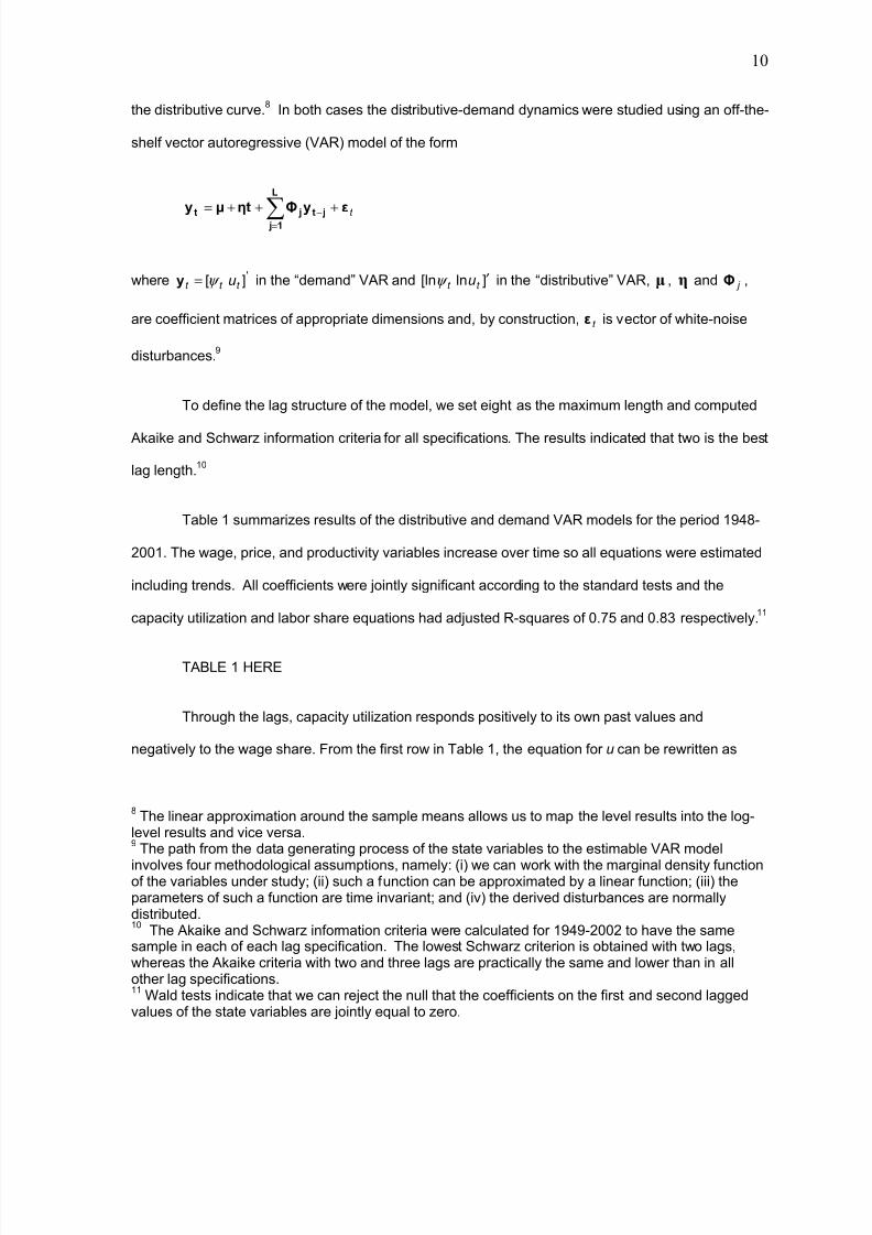
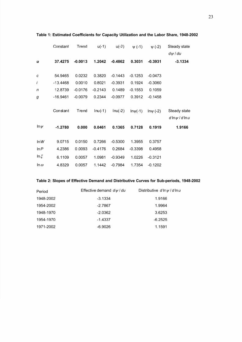
Table 1 summarizes results of the distributive and demand VAR models for the period 1948-

2001. The wage, price, and productivity variables increase over time so all equations were estimated

including trends. All coefficients were jointly significant according to the standard tests and the

capacity utilization and labor share equations had adjusted R-squares of 0.75 and 0.83 respectively.11

TABLE 1 HERE

Through the lags, capacity utilization responds positively to its own past values and

negatively to the wage share. From the first row in Table 1, the equation for u can be rewritten as

8 The linear approximation around the sample means allows us to map the level results into the log-

level results and vice versa.9 The path from the data generating process of the state variables to the estimable VAR model

involves four methodological assumptions, namely: (i) we can work with the marginal density functionof the variables under study; (ii) such a function can be approximated by a linear function; (iii) theparameters of such a function are time invariant; and (iv) the derived disturbances are normallydistributed.10

The Akaike and Schwarz information criteria were calculated for 1949-2002 to have the samesample in each of each lag specification. The lowest Schwarz criterion is obtained with two lags,whereas the Akaike criteria with two and three lags are practically the same and lower than in allother lag specifications.11

Wald tests indicate that we can reject the null that the coefficients on the first and second laggedvalues of the state variables are jointly equal to zero.



11

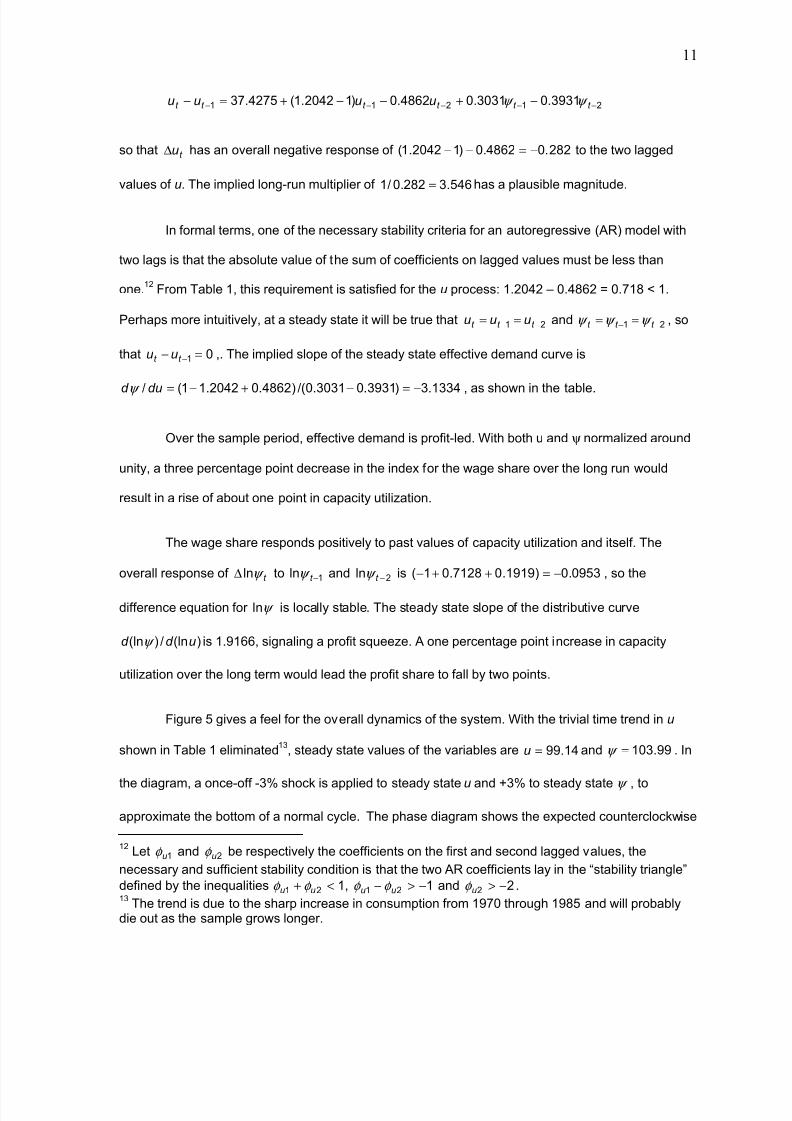
21211 3931.03031.04862.0)12042.1(4275.37 −−−−− −+−−+=− t t t t t t uuuu ψ ψ

so that t u∆ has an overall negative response of 282.04862.0)12042.1( −=−− to the two lagged

values of u. The implied long-run multiplier of 546.3282.0/1 = has a plausible magnitude.

In formal terms, one of the necessary stability criteria for an autoregressive (AR) model with

two lags is that the absolute value of the sum of coefficients on lagged values must be less than

one.12

From Table 1, this requirement is satisfied for the u process: 1.2042 – 0.4862 = 0.718 < 1.

Perhaps more intuitively, at a steady state it will be true that 21 −− == t t t uuu and 21 −− == t t t ψ ψ ψ , so

that 01 =− −t t uu ,. The implied slope of the steady state effective demand curve is

1334.3)3931.03031.0/()4862.02042.11(/ −=−+−=dud ψ , as shown in the table.

Over the sample period, effective demand is profit-led. With both u and ψ normalized around

unity, a three percentage point decrease in the index for the wage share over the long run would

result in a rise of about one point in capacity utilization.

The wage share responds positively to past values of capacity utilization and itself. The

overall response of t ψ ln∆ to 1ln −t ψ and 2ln −t ψ is 0953.0)1919.07128.01( −=++− , so the

difference equation for ψ ln is locally stable. The steady state slope of the distributive curve

)(ln/)(ln ud d ψ is 1.9166, signaling a profit squeeze. A one percentage point increase in capacity

utilization over the long term would lead the profit share to fall by two points.

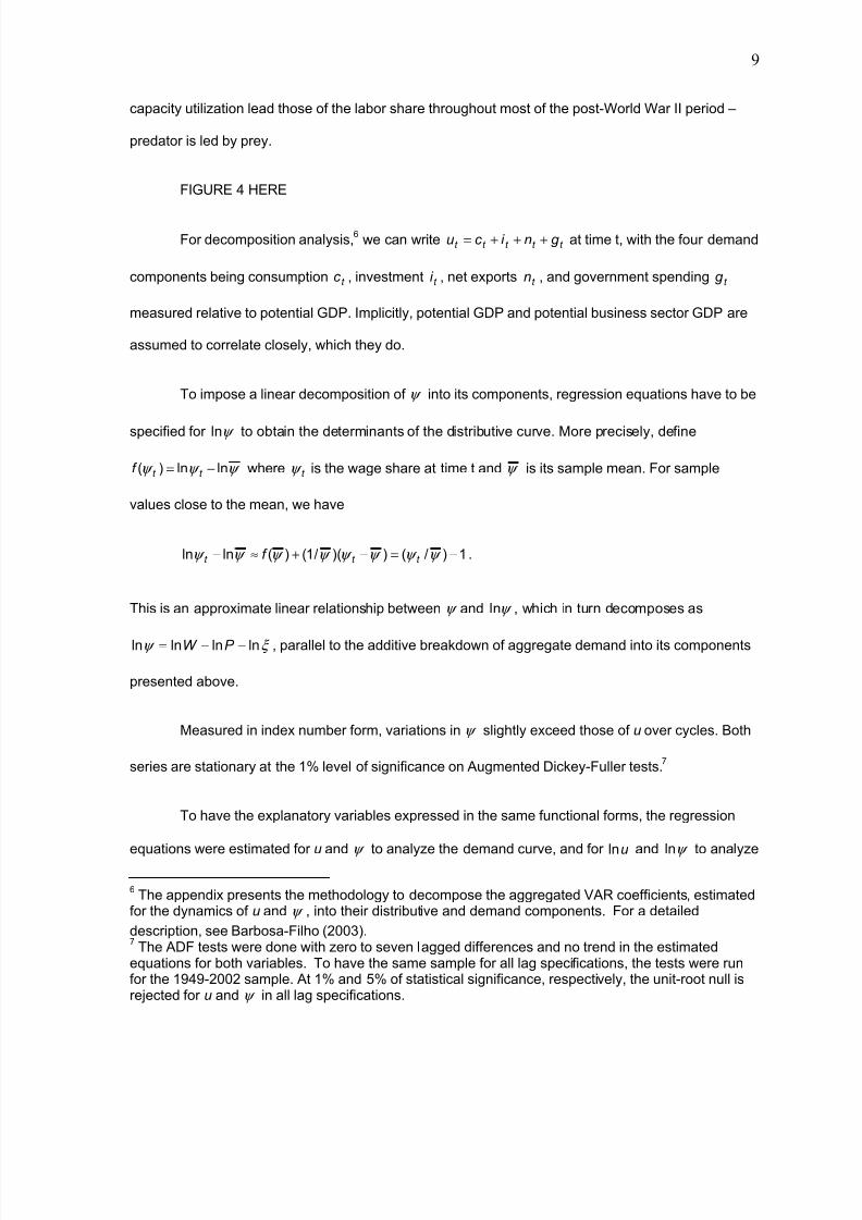
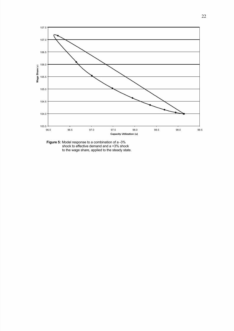
Figure 5 gives a feel for the overall dynamics of the system. With the trivial time trend in u

shown in Table 1 eliminated13

, steady state values of the variables are 14.99=u and 99.103=ψ . In

the diagram, a once-off -3% shock is applied to steady state u and +3% to steady state ψ , to

approximate the bottom of a normal cycle. The phase diagram shows the expected counterclockwise

12 Let 1uφ and 2uφ be respectively the coefficients on the first and second lagged values, the

necessary and sufficient stability condition is that the two AR coefficients lay in the “stability triangle”

defined by the inequalities 121 <+ uu φ φ , 121 −>− uu φ φ and 22 −>uφ .13

The trend is due to the sharp increase in consumption from 1970 through 1985 and will probablydie out as the sample grows longer.



12

pattern. The state variables return close to the steady state after eight quarters (and cycle in the

vicinity thereafter).

FIGURE 5 HERE

Table 2 presents the slopes of the effective demand and distributive curves for the “Golden

Age” period that began after WWII and ended in the early 1970s, and thereafter. A convenient

breakpoint is the year 1970, which contained the trough of an NBER business cycle. The initial year is

alternatively 1948 or 1954 (the latter a trough year which omits the immediate post-WWII and Korean

War periods).

TABLE 2 HERE

Over both 1948-2001 and 1954-2001, demand is profit-led and there is a profit squeeze. Pre-

1970, the demand effect is stronger (a two percentage point decrease in ψ would make u increase by

one point or more in the long run), and weakens during 1971-2001. Further sample splits suggest that

demand may have shifted to being wage-led during the 1970s but was profit-led in the preceding and

following decades.14

However, the number of observations per decade is too low to make a solid

case.

During 1954-1970, the distributive curve takes a negative slope and the difference equation

for ψ ln is locally unstable as in the lower diagram of Figure 3.

Otherwise, the qualitative characteristics of the economy are described by the upper diagram

in Figure 3. It follows that “permanent” distributive shocks favorable to labor (upward shifts of the

distributive curve) lead to an increase in the labor share at the expense of a reduction in capacity

utilization; and that permanent positive demand shocks (upward shifts of the demand curve) lead to

increases in capacity utilization and the labor share. Along the lines of Figure 5, convergence to a

“new” long run intersection of the Effective Demand and Distributive curves would be cyclical.

14 Blecker (1991) suggests that the Reagan fiscal package may have pushed the economy in a profit-

led direction during the 1980s.



13

As discussed above, it is possible to use VAR estimation subject to adding-up restrictions to

express the demand components of u and the price/productivity components of ψ ln as functions of

lagged values of these two variables (for details on the procedure, see the Appendix). The results of

these reduced form estimates are also shown in Table 1.

The estimated coefficients suggest that t c , or the ratio of private consumption to potential

GDP, has a positive trend and is pro-cyclical.15

Investment t i also varies pro-cyclically. Net exports

t n have a downward trend and respond negatively to both capacity utilization and the wage share

(interpreted as an index of labor costs). Government spending t g also has a negative trend, and

responds positively to u and ψ . In the aggregate, the profit-led components predominate and, by

construction, there is a trivial overall trend in u (see footnote 13).

Trends are stronger in the logs of W , P , and ξ . The real wage increases at approximately

0.57% per quarter in 1948-2002, due to trend money wage growth outstripping the trend in the price

level. Labor productivity growth also grows at 0.57%, stabilizing the wage share.

The coefficients for ω ln and ξ ln are consistent with the descriptions above for the long

period 1948-2001. As already noted, during 1954-70, the sum of the coefficients on ψ ln in the

productivity equation is -1.18, giving rise to the form of cyclical dynamics illustrated in the lower

diagram of Figure 3.

The nominal wage responds positively over two lags to capacity utilization, along Phillips

curve lines, and also responds positively to the wage share. The price level responds counter-

cyclically to capacity utilization and (over two lags) is largely unaffected by unit labor costs as

measured by ψ .

15 Net lending by households, or their savings less investment, varies counter-cyclically, consistent

with the econometric result (Taylor, 2003).



14

3. Conclusions

In summary:

There are rather regular counter-clockwise cycles involving capacity utilization u (horizontal

axis) and the labor share ψ (vertical axis) in the US economy post-WWII. In Lotka-Volterra terms,

ψ can be interpreted as a predator variable and u as prey.

The cycles can be rationalized in phase diagram terms as being driven by dynamics around

schedules along which 0=u& and 0=ψ & . The former can be interpreted in terms of effective demand

- specifically demand responds negatively to ψ or is profit-led. The latter can be interpreted in

distributive terms – in the long run the wage share rises along with capacity utilization or the

functional distribution is subject to a profit squeeze.

Econometric results suggest that all components of demand contribute to its profit-led

character. Real wage and labor productivity dynamics over the cycle are the main driving force

behind the distributive profit squeeze. Across cycles, both the real wage and labor productivity grow

at about 0.57% per quarter, holding the wage share broadly stable.

Modeling the cycle in the (u, ψ ) plane provides a parsimonious description of demand and

distributive dynamics that is consistent with the view of macroeconomics embedded in the work of

Kalecki and many subsequent followers.

Appendix on estimating demand components and wage and price responses

The VAR model for u and ψ can be written as

ttt εΓxy += , (A1)

where naturally [ ]21 ΦΦηµΓ = and ]1[' '2t

'1t yyx −−= t t . The Ordinary Least Squares (OLS) and

Maximum Likelihood (ML) estimator of Γ (Hamilton, 1994) is given by:



15

1

ˆ−

==

∑

∑=

T

1t

'tt

T

1t

'tt xxxyΓ . (A2)

Let )('t t t t t t ng i c ψ =z be the vector containing the labor share and the demand-potential

output ratios that add up to t u . The “demand” VAR implicit in the equation for u in (A1) is given by

the following regression:

ttt νΠwz += , (A3)

where Π is a 4x12 coefficient matrix and ]1[ '2

'−−= t t t zzw '

1t . In other words, the demand VAR is a

regression of the labor share and the demand components on their past values and a constant and a

time trend. In relation to (A1), the crucial difference is that (A3) breaks u in its four components.

By analogy with (A2), the OLS and ML estimator of Π is

1

ˆ−

==

∑

∑=

T

1t

'tt

T

1t

'tt wwwzΠ (A4)

By definition:

tt Gwx = (A5)

where G is a 6x12 matrix of constant terms that maps tw into tx . Substituting (A5) in (A2) and after

some algebraic operations we obtain

FΠHΓ ˆˆ = , (A6)

where

=

1

0

00

11

00

11H

and



16

1−

==

∑

∑= '

T

1t

'tt

'T

1t

'tt GwwGGwwF

The purpose of (A6) is to find how each “aggregated” coefficient of the first line of (A1) can be

decomposed in terms of the “disaggregated” coefficients of the first four lines of (A3). In other words,

the purpose is to know how much of the aggregated demand coefficients come from consumption,

investment, net exports and government expenditures. Given the sample values of w , F is a matrix of

fixed weights and the decomposition of the aggregated demand results is implicit in the right-hand

side of (A6).

By analogy, the same method applies for the decomposition of the “aggregated coefficients”

of the labor-share equation, provided that we use logs instead of levels to assure that the wage, price

and productivity variables add up to the labor share variable.

References

Barbosa-Filho, Nelson H. (2001) “Income Distribution and Demand Fluctuations in the US Economy”in Essays on Structuralist Macroeconomics, New York NY: Department of Economics, NewSchool University (unpublished Ph. D. dissertation)

Barbosa-Filho, Nelson H. (2003) “A Note on Aggregated and Disaggregated Estimates of Vector

Autoregressive Models,” New York: Center for Economic Policy Analysis, New SchoolUniversity

Bhaduri, Amit, and Stephen A. Marglin (1990) "Unemployment and the Real Wage: The EconomicBasis for Contesting Political Ideologies,” Cambridge Journal of Economics, 14: 375-393

Blecker, Robert A. (2002) "Distribution, Demand, and Growth in Neo-Kaleckian Macro Models," inMark Setterfield (ed.), Demand-Led Growth: Challenging the Supply-Side Vision of the LongRun, Northhampton MA: Edward Elgar

Bowles, Samuel, and Robert Boyer (1995) "Wages, Aggregate Demand, and Employment in an OpenEconomy: an Empirical Investigation," in Gerald A. Epstein and Herbert A. Gintis (eds.)Macroeconomic Policy after the Conservative Era, Cambridge: Cambridge University Press

Boddy, Raford, and James R. Crotty (1975) "Class Conflict and Macro Policy: The Political BusinessCycle," Review of Radical Political Economics, 7 (1): 1-19

Bowles, Samuel, David Gordon, and Thomas Weisskopf (1990) After the Wasteland: A DemocraticEconomics for the Year 2000 , Armonk NY: M. E. Sharpe

Desai, Meghnad (1973) "Growth Cycles and Inflation in a Model of Class Struggle,” Journal ofEconomic Theory , 6 : 527-545

Dutt, Amitava Krishna (1984) "Stagnation, Income Distribution, and Monopoly Power," CambridgeJournal of Economics, 8 : 25-40



17

Goldstein, Jonathan P. (1996) "The Empirical Relevance of the Cyclical Profit Squeze: AReassertion," Review of Radical Political Economics, 28 (4): 55-92

Goodwin, Richard M. (1967) "A Growth Cycle," in C. H. Feinstein (ed.) Socialism, Capitalism, andGrowth, Cambridge: Cambridge University Press

Gordon, David M. (1995) "Growth, Distribution, and the Rules of the Game: Social Structuralist MacroFoundations for a Democratic Economic Policy," in Gerald A. Epstein and Herbert A. Gintis(eds.) Macroeconomic Policy after the Conservative Era, Cambridge: Cambridge UniversityPress

Hamilton, James. D. (1994) Time Series Analysis. Princeton: University of Princeton Press.

Kaldor, Nicholas (1956) "Alternative Theories of Distribution," Review of Economic Studies, 23: 83-100

Kaldor, Nicholas (1957) "A Model of Economic Growth," Economic Journal , 67 : 591-624

Kalecki, Michal (1971) Selected Essays on the Dynamics of the Capitalist Economy: 1933-1970, Cambridge: Cambridge University Press

Lotka, Alfred Y. (1925) Elements of Physical Biology , Baltimore: Williams and Wilkins

Marglin, Stephen A. (1984) Growth, Distribution, and Prices, Cambridge MA: Harvard UniversityPress

Rowthorn, Robert E. (1982) "Demand, Real Wages, and Economic Growth," Studi Economici, 18 : 2-53

Steindl, Josef (1952) Maturity and Stagnation in American Capitalism, Oxford: Basil Blackwell

Taylor, Lance (2003). Reconstructing Macroeconomics: Structuralist Proposals and Critiques of theMainstream, Cambridge MA: Harvard University Press

Volterra, Vito (1931) Leçons sur la Théorie Mathématique de la Lutte por la Vie, Paris: Gauthier-VillarNotes



18

Figure 1 – US Economy 1950-2002. Labor share of income = 100x(labor compensation/nationalincome); global rate of capacity utilization = 100x(real GDP/ real potential GDP); real potential GDP =Hodrick-Prescott trend of real GDP; source: Bureau of Economic Analysis’ NIPA tables 1.2 and 1.14.

63

65

67

69

71

73

75

94 95 96 97 98 99 100 101 102 103 104

global rate of capacity utilization

l a b o r s h a r e o f n a t i o n a l i n c o m

1950

1967

1982

2002

1979

1954

19581996

1970

1975



19

Figure 2 - US Economy: 1929-2002. Labor share of income = 100x(labor compensation/nationalincome); global rate of capacity utilization = 100x(real GDP/ real potential GDP); real potential GDP =Hodrick-Prescott trend of real GDP; source: Bureau of Economic Analysis’ NIPA tables 1.2 and 1.14.

58

60

62

64

66

68

70

72

74

84 89 94 99 104 109 114 119 124

global rate of capacity utlization

l a b o r s h a r e o

f n a t i o n a l i n c o m e

1929

1933

1938

1944

1950

1967

2002

19821979



20

Wage share

Figure 9.2: AstructuralistGoodwinmodel,withstable(upper)and

unstable(lower)wagesharedynamics

ψ

Wage share

Output/capitalratio u

ψ

Output/capitalratio u

Distributive

Effectivedemand

Effectivedemand

Distributive

Figure 3: A structuralist Goodwinmodel, with stable (upper) and

unstable (lower) wage share

dynamics



21

Figure 4 - Business Sector of the US Economy: 1947-02. Labor share index = (business laborcompensation per hour)/[(business price deflator)x(business output per hour)], all series calculatedwith 1992=100; global rate of capacity utilization = 100x(real business output)/(real potential businessoutput); real potential business output = Hodrick-Prescott trend of real business output; source:Bureau of Labor Statistics’ productivity and costs series.

95

96

97

98

99

100

101

102

103

104

105

106

94 96 98 100 102 104 106

global rate of capacity utilization

i n d e x o f t h e l a b o r s h a r e o f i n c o m e ( 1 9 9 2 = 1 0 0 )

1947

1949

1951

1953

2002

1996

1982

1973

1970

19751966

2000

1960



22

Figure 5: Model response to a combination of a -3%shock to effective demand and a +3% shockto the wage share, applied to the steady state.

103.5

104.0

104.5

105.0

105.5

106.0

106.5

107.0

107.5

96.0 96.5 97.0 97.5 98.0 98.5 99.0 99.5

Capacity Utilization (u)

W a g e S h a r e ( ψ )



23

Table 1: Estimated Coefficients for Capacity Utilization and the Labor Share, 1948-2002

Constant Trend u(-1) u(-2) ψ (-1) ψ (-2)

Steady state

dud /ψ

u 37.4275 -0.0013 1.2042 -0.4862 0.3031 -0.3931 -3.1334

c 54.9465 0.0232 0.3820 -0.1443 -0.1253 -0.0473

i -13.4468 0.0010 0.8021 -0.3931 0.1924 -0.3060

n 12.8739 -0.0176 -0.2143 0.1489 -0.1553 0.1059

g -16.9461 -0.0079 0.2344 -0.0977 0.3912 -0.1458

Constant Trend lnu(-1) lnu(-2) lnψ (-1) lnψ (-2) Steady state

ud d ln/lnψ

ψ ln -1.2780 0.000 0.0461 0.1365 0.7128 0.1919 1.9166

W ln 9.0715 0.0150 0.7266 -0.5300 1.3955 0.3757

P ln 4.2386 0 .0093 -0.4176 0.2684 -0.3398 0.4958

ξ ln 6.1109 0.0057 1.0981 -0.9349 1.0226 -0.3121

ω ln 4.8329 0.0057 1.1442 -0.7984 1.7354 -0.1202

Table 2: Slopes of Effective Demand and Distributive Curves for Sub-periods, 1948-2002

Period Effective demand dud /ψ Distributive ud d ln/lnψ

1948-2002 -3.1334 1.9166

1954-2002 -2.7867 1.9964

1948-1970 -2.0362 3.6253

1954-1970 -1.4337 -6.2525

1971-2002 -6.9026 1.1591

Distributive and Demand Cycles in the US Economy.pdf

Documents

Transcript of Distributive and Demand Cycles in the US Economy.pdf