Micro-Demand Systems Analysis of Non-Alcoholic

Beverages in the United States: An Application of Econometric Techniques Dealing With Censoring

by

Pedro A. Alviola IV Program Associate

Department of Agricultural Economics and Agribusiness,

University of Arkansas, Fayetteville, AR 72701

Oral Capps Jr.

Executive Professor Holder of the Southwest Dairy Marketing Endowed Chair

Department of Agricultural Economics, Texas A&M University,

College Station, TX 77843-2124.

and Ximing Wu

Associate Professor, Department of Agricultural Economics,

Texas A&M University, College Station, TX 77843-2124.

Selected Paper prepared for presentation at the Agricultural & Applied Economics Association’s 2010 AAEA, CAES & WAEA Joint Annual Meeting, Denver, Colorado,

July 25-27, 2010. Copyright 2010 by Pedro A Alviola IV, Oral Capps, Jr and Ximing Wu. All rights reserved. Readers may make verbatim copies of this document for non-commercial purposes by any means, provided this copyright notice appears on all such copies

Micro-Demand Systems Analysis of Non-Alcoholic

Beverages in the United States: An Application of Econometric Techniques Dealing With Censoring

Abstract

A censored Almost Ideal Demand System (AIDS) and a Quadratic Almost Ideal Demand

System (QUAIDS) were estimated in modeling non-alcoholic beverages. Five estimation

techniques were used, including the conventional Iterated Seemingly Unrelated

Regression (ITSUR), two-stage methods such as the Heien and Wessells (1990) and the

Shonkwiler and Yen (1999) approaches, the generalized maximum entropy method and

the Amemiya-Tobin framework of Dong, Gould and Kaiser (2004). Our results based on

various specifications and estimation techniques are quantitatively similar and indicate

that price elasticity estimates have a greater variability in more highly censored non-

alcoholic beverage items such as tea, coffee and bottled water as opposed to less censored

non-alcoholic beverage items such as carbonated softdrinks, milk and fruit juices.

Key Words: Censored demand systems, AIDS, QUAIDS, two- step methods, generalized

maximum entropy, Amemiya-Tobin Framework, and non-alcoholic beverages

1

The move towards different diets that favor nutritious foods has in recent years led to the

emergence of healthier and natural food choices. In particular, manufacturers and

retailers have been responsive in introducing new products to the non-alcoholic beverage

industry, especially juices, energy drinks and others. This paper focuses on the

interdependencies and demand for certain non-alcoholic beverages, namely; fruit juices,

tea, coffee, carbonated soft drinks, milk and bottled water. In the case of the non-

alcoholic beverage complex, these products have different levels of market penetration.

Consequently, the consumption/expenditure variables associated with these non-alcoholic

beverages are censored at zero. That is, certain households have zero expenditure, but the

corresponding information on household characteristics, which forms the basis of the

explanatory variables are often readily observed. Several competing estimation methods

have been developed in order to address the censoring issue in the estimation of micro-

demand systems. As microdata become increasingly available and more detailed, the

estimation of micro-demand systems at the household level becomes problematic due to

censoring. To our knowledge, no prior research has been done in terms of comparing

these respective approaches with regard to a particular data set.

In this study, the demand systems employed were the Quadratic Almost Ideal

Demand System (QUAIDS) (Banks, Blundell and Lewbel, 1997) and Almost Ideal

Demand System (AIDS) (Deaton and Mulbauer, 1980). The advantages of the QUAIDS

model are its flexibility in incorporating nonlinear effects and interactions of price and

expenditures in the demand relationships. Since the data used are at the household level,

censoring typically is observed as some households report expenditures of a beverage

2

product say coffee and none on say bottled water. Thus, in order to model the censoring

problem in demand systems, the research utilized estimation procedures including two-

step estimators (Heien and Wessells, 1990; Shonkwiler and Yen, 1999), the maximum

entropy method (Golan, Judge and Miller, 1996) and the maximum simulated likelihood

estimation method (Dong, Gould and Kaiser, 2004). The iterated seemingly unrelated

regression (ITSUR) estimation without adjustments for censoring serves as a baseline of

comparison for the aforementioned estimation techniques. Finally, the source of data is

the 1999 Nielsen Homescan Panel due to its vast array of household demographic

information.

Literature Review

The Quadratic Almost Ideal Demand System (QUAIDS) commonly is used in applied

work. For example, Dhar and Foltz (2005) utilized a Quadratic AIDS model to estimate

values and benefits derived from recombinant bovine somatotropin (rBST)-free milk,

organic milk and unlabelled milk. Their study relied on the use of time-series scanner

data pertaining to milk consumption from 12 key cities in the United States. Their

findings indicate that rBST-free milk and organic milk are complements, while

conventional milk and rBST-free milk as well as conventional milk and organic milk are

substitutes. The respective own-price elasticity estimates were -4.40 for rBST-free milk, -

1.37 for organic milk and -1.04 for conventional milk.

Likewise, a study done by Mutuc, Pan and Rejesus (2007) investigated household

demand for vegetables in the Philippines using the QUAIDS model. Their findings

indicated significant differences in expenditure elasticities between rural and urban areas

3

whereas for the respective own-price and cross-price elasticities, no significant variations

across rural and urban areas were evident. Dhar and Foltz (2005) encountered no

censoring issues, and subsequently used the Full Information Maximum Likelihood

(FIML) estimator. In Mutuc, Pan and Rejesus (2007) work, censoring problems occurred

because of the presence of zero expenditures on some vegetable commodities consumed

by the sample of households. Hence they relied upon the the Shonkwiler and Yen (1999)

two-step procedure to circumvent the censoring issue.

The Heien and Wessells (1990) approach mimics the Heckman two-stage method

by first estimating probit models to compute inverse Mills ratios for each commodity.

Subsequently, these ratios are incorporated into the second-step SUR estimation of the

demand system. On the other hand, Shonkwiler and Yen (1999) proposed a consistent

estimation procedure that utilizes a probit estimator in the first step. Subsequently, the

cumulative distribution function (cdf) is used to multiply the covariates in the demand

model and the probability density function (pdf) is included as an independent variable in

the second step. Both methods fall under the purview of utilizing two-step estimators.

While the Shonkwiler and Yen approach worked well with the problem of zero

expenditures, Arndt, Liu and Preckel (1999) claimed that it had limitations with respect

to dealing with corner solutions. Several studies including Arndt (1999) and Golan,

Perloff and Shen (2001) propose an alternative maximum entropy approach to estimate

censored demand systems. This approach allows for consistent and efficient estimation of

demand systems without putting any restrictions on the error terms. Other researchers

4

such as Meyerhoefer, Ranney and Sahn (2005) use the general method of moments

(GMM) estimator to address censoring problems in demand systems estimation.

Several studies have criticized the two-step methods stating that the “adding up”

restriction in estimating share equations in censored demand systems is ignored (Dong,

Gould and Kaiser, 2004; Yen, Lin and Smallwood, 2003). Together with Golan, Perloff

and Shen (2001), these classes of estimators fall under the Amemiya-Tobin framework

where the former does not employ maximum likelihood estimation in evaluating

multivariate probability integrals. Dong, Gould and Kaiser (2004) and Yen, Lin and

Smallwood (2003) utilize numerical methods such as maximum and quasi-maximum

simulated likelihood estimation in approximating the likelihood function. The literature

regarding the use of alternative estimation techniques such as Bayesian and non-

parametric approaches on micro-demand system estimation have been limited (Tiffin and

Aquiar, 1995).

Methodology

Almost Ideal Demand System (AIDS) Model

This research utilizes the AIDS (Deaton and Mulbauer, 1980) in the estimation of the

demand for six non-alcoholic beverages, namely: fruit juices, tea, coffee, carbonated soft

drinks, bottled water and milk. Equation (1) describes the general specification of the

AIDS model where pi and wi are the price and budget share of the ith beverage

commodity. The average budget share wi is computed as piqi/M where M = ∑piqi is the

total expenditure on the six aforementioned non-alcoholic beverages. The parameters of

this system are αi, γi and βi, respectively. One can also incorporate household

5

demographic characteristics into the demand system thru the intercept parameter αi.

These variables include household size, household income, race and region. Also, a

seasonality component was added.

(1) ij

ijijii paMpw εβγα +⎥

⎦

⎤⎢⎣

⎡++= ∑

=

6

1 )(lnln , i-1,2,..6

where:

,lnln5.0ln)(ln6

1∑∑∑ ++=

= jjiij

ii

iio ppppa γαα and,

RgSeasonRaceIncHHsize iiiiiii 54321* ααααααα +++++=

In our study, we incorporate selected demographic variables namely household

size (HHsize), income (Inc), race (Race), seasonality (Season) and region (Rg) in the

analysis. Likewise, the classical theoretical restrictions of adding up, homogeneity and

symmetry were imposed in the estimation of the AIDS demand system:

Adding up:∑=

=n

ii

11α , 0

1=∑

=

n

iiβ , 0

1

=∑=

n

jijγ

Homogeneity: 01

=∑=

n

jijγ

Symmetry: jiij γγ =

Quadratic Almost Ideal Demand System (QUAIDS) Model

The Quadratic Almost Ideal Demand System (QUAIDS) model (Banks, Blundell and

Lewbel, 1997) also is utilized in this demand analysis. The advantages of using this

model over competing flexible demand systems is its unparalleled capability of

incorporating non-linear effects and interactions of price and expenditures on the demand

6

specifications. The mathematical representation of the QUAIDS demand system is as

follows:

(2) ii

jijijii pa

Mpbpa

Mpw ελβγα +⎥⎦

⎤⎢⎣

⎡⎟⎟⎠

⎞⎜⎜⎝

⎛+⎥

⎦

⎤⎢⎣

⎡++= ∑

=

26

1 )(ln

)()(lnln , i-1,2,.,6

where:

andppb

ppppa

n

ii

jjiij

ii

n

iio

i ,)(

,lnln5.0ln)(ln

1

1

∏

∑∑∑

=

=

=

++=

β

γαα

.54321* RgSeasonRaceIncHHsize iiiiiii ααααααα +++++=

The QUAIDS model is a generalization of the AIDS model. Also, if the null

hypothesis that λ1 = λ2 =…= λ6=0 is rejected then the QUAIDS model is a superior

model at least statistically relative to the AIDS model system. In this research, the

intercept parameter αi incorporates selected household demographic characteristics just as

with the AIDS model. Adding up, homogeneity conditions and symmetry conditions also

are imposed on the demand system as follows;

Adding up:∑=

=n

ii

11α , 0

1=∑

=

n

iiβ , 0

1

=∑=

n

jijγ , 0

1=∑

=

n

iiλ

Homogeneity: 01

=∑=

n

jijγ

Symmetry: jiij γγ =

7

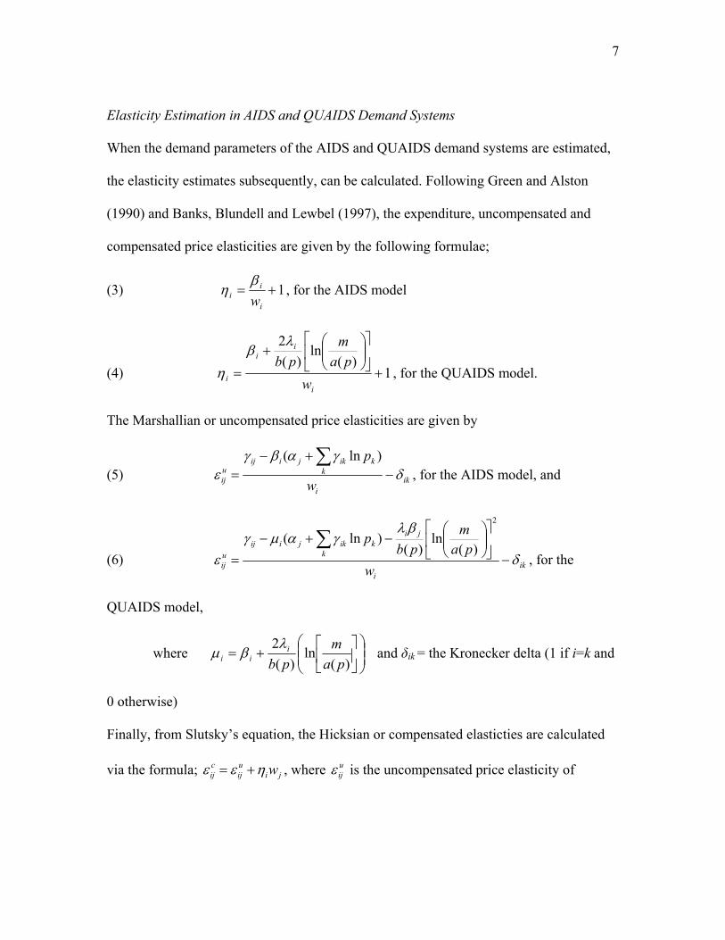
Elasticity Estimation in AIDS and QUAIDS Demand Systems

When the demand parameters of the AIDS and QUAIDS demand systems are estimated,

the elasticity estimates subsequently, can be calculated. Following Green and Alston

(1990) and Banks, Blundell and Lewbel (1997), the expenditure, uncompensated and

compensated price elasticities are given by the following formulae;

(3) 1+=i

ii w

βη , for the AIDS model

(4) 1)(

ln)(

2

+⎥⎦

⎤⎢⎣

⎡⎟⎟⎠

⎞⎜⎜⎝

⎛+

=i

ii

i wpa

mpbλ

βη , for the QUAIDS model.

The Marshallian or uncompensated price elasticities are given by

(5) iki

kk

ikjiijuij w

pδ

γαβγε −

+−=

∑ )ln(, for the AIDS model, and

(6) iki

jik

kikjiij

uij w

pam

pbp

δ

βλγαμγ

ε −⎥⎦

⎤⎢⎣

⎡⎟⎟⎠

⎞⎜⎜⎝

⎛−+−

=∑

2

)(ln

)()ln(

, for the

QUAIDS model,

where ⎟⎟⎠

⎞⎜⎜⎝

⎛⎥⎦

⎤⎢⎣

⎡+=

)(ln

)(2

pam

pbi

iiλ

βμ and δik = the Kronecker delta (1 if i=k and

0 otherwise)

Finally, from Slutsky’s equation, the Hicksian or compensated elasticties are calculated

via the formula; jiuij

cij wηεε += , where u

ijε is the uncompensated price elasticity of

8

beverage i with respect to beverage j and iη is the budget elasticity of beverage i. The

term wj is the mean budget share of beverage j.

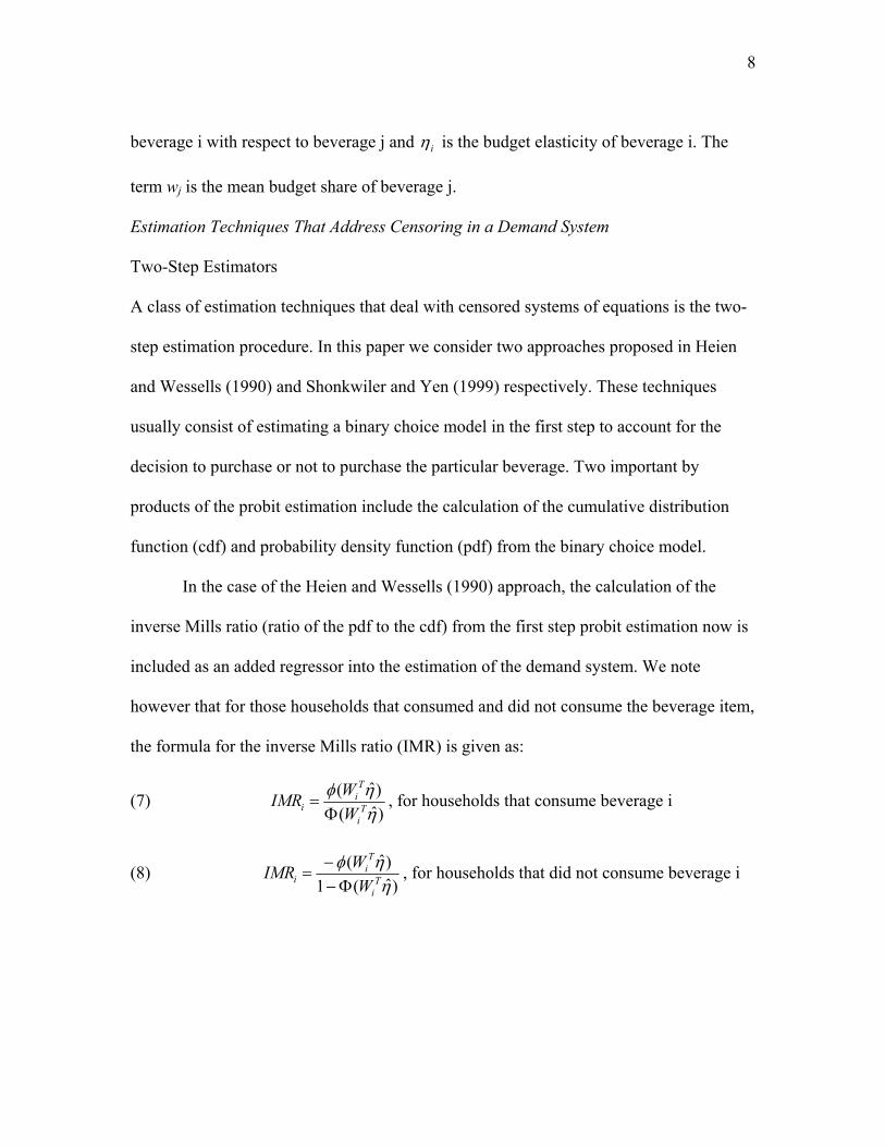
Estimation Techniques That Address Censoring in a Demand System

Two-Step Estimators

A class of estimation techniques that deal with censored systems of equations is the two-

step estimation procedure. In this paper we consider two approaches proposed in Heien

and Wessells (1990) and Shonkwiler and Yen (1999) respectively. These techniques

usually consist of estimating a binary choice model in the first step to account for the

decision to purchase or not to purchase the particular beverage. Two important by

products of the probit estimation include the calculation of the cumulative distribution

function (cdf) and probability density function (pdf) from the binary choice model.

In the case of the Heien and Wessells (1990) approach, the calculation of the

inverse Mills ratio (ratio of the pdf to the cdf) from the first step probit estimation now is

included as an added regressor into the estimation of the demand system. We note

however that for those households that consumed and did not consume the beverage item,

the formula for the inverse Mills ratio (IMR) is given as:

(7) )ˆ()ˆ(

ηηφ

Ti

Ti

i WWIMR

Φ= , for households that consume beverage i

(8) )ˆ(1

)ˆ(ηηφT

i

Ti

i WWIMR

Φ−−

= , for households that did not consume beverage i

9

where, )ˆ( ηφ iW , )ˆ( ηiWΦ and Wi correspond to the pdf , cdf and vector of socio-

demographic variables including income, race and region. Thus, the Heien and Wessells

(1990) two-step approach of estimating a demand system can be represented as:

(9) iii

n

jijijii IMR

paMpw ευβγα ++⎥

⎦

⎤⎢⎣

⎡++= ∑

=1 )(lnln , for the AIDS model

(10) iiii

n

jijijii IMR

paM

pbpaMpw ευλβγα ++⎥

⎦

⎤⎢⎣

⎡⎟⎟⎠

⎞⎜⎜⎝

⎛+⎥

⎦

⎤⎢⎣

⎡++= ∑

=

2

1 )(ln

)()(lnln , for the

QUAIDS model.

On the other hand, the Shonkwiler and Yen (1999) consistent two-step approach

utilizes the calculated cdf to multiply the entire right hand side variables of the share

equation and include the pdf as an additional regressor in the system of budget shares.

This formulation can be represented as:

(11) iiij

n

jijiii W

paMpWw εηφβγαη ++⎥

⎦

⎤⎢⎣

⎡⎟⎟⎠

⎞⎜⎜⎝

⎛++Φ= ∑

=

)()(

lnln)(1

, for the AIDS model

(12) iii

ij

n

jijiii W

paM

pbpaMpWw εηφλβγαη ++

⎥⎥⎦

⎤

⎢⎢⎣

⎡⎟⎟⎠

⎞⎜⎜⎝

⎛⎟⎟⎠

⎞⎜⎜⎝

⎛+⎟⎟

⎠

⎞⎜⎜⎝

⎛++Φ= ∑

=

)()(

ln)()(

lnln)(2

1

,

for the QUAIDS model.

Dong, Gould and Kaiser Approach (2004)

We also used the Dong, Gould and Kaiser (2004) approach, a variant of the Amemiya-

Tobin model in estimating a censored AIDS model. In this approach the AIDS demand

model can be written as:

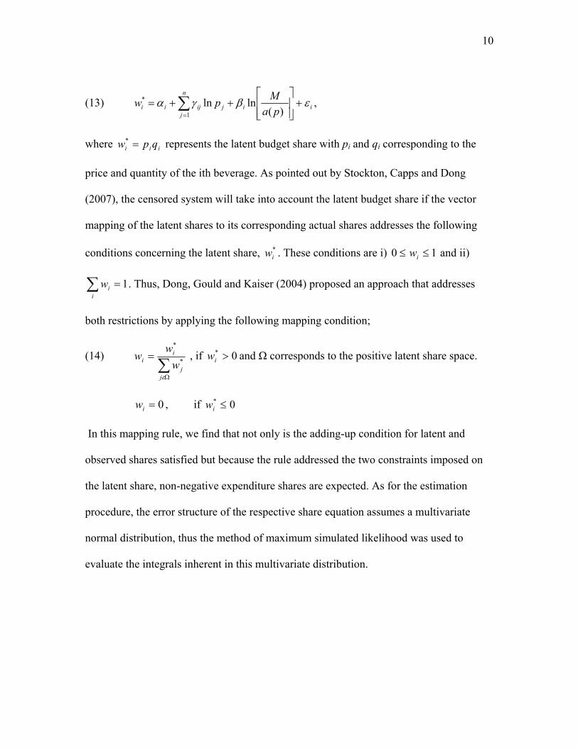
10

(13) i

n

jijijii pa

Mpw εβγα +⎥⎥⎦

⎤

⎢⎢⎣

⎡++= ∑

=1

*

)(lnln ,

where iii qpw =* represents the latent budget share with pi and qi corresponding to the

price and quantity of the ith beverage. As pointed out by Stockton, Capps and Dong

(2007), the censored system will take into account the latent budget share if the vector

mapping of the latent shares to its corresponding actual shares addresses the following

conditions concerning the latent share, *iw . These conditions are i) 10 ≤≤ iw and ii)

1=∑i

iw . Thus, Dong, Gould and Kaiser (2004) proposed an approach that addresses

both restrictions by applying the following mapping condition;

(14) ∑Ω

=

εjj

ii w

ww *

*

, if 0* >iw and Ω corresponds to the positive latent share space.

0=iw , if 0* ≤iw

In this mapping rule, we find that not only is the adding-up condition for latent and

observed shares satisfied but because the rule addressed the two constraints imposed on

the latent share, non-negative expenditure shares are expected. As for the estimation

procedure, the error structure of the respective share equation assumes a multivariate

normal distribution, thus the method of maximum simulated likelihood was used to

evaluate the integrals inherent in this multivariate distribution.

11

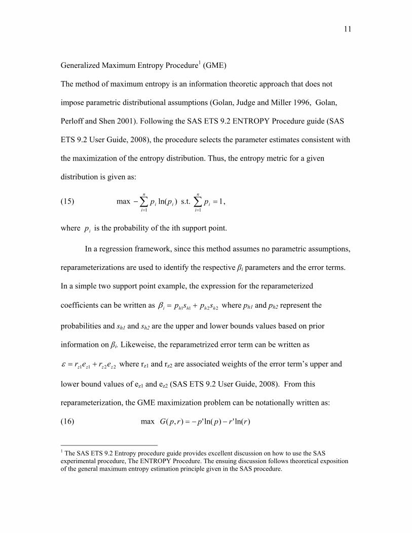
Generalized Maximum Entropy Procedure1 (GME)

The method of maximum entropy is an information theoretic approach that does not

impose parametric distributional assumptions (Golan, Judge and Miller 1996, Golan,

Perloff and Shen 2001). Following the SAS ETS 9.2 ENTROPY Procedure guide (SAS

ETS 9.2 User Guide, 2008), the procedure selects the parameter estimates consistent with

the maximization of the entropy distribution. Thus, the entropy metric for a given

distribution is given as:

(15) max )ln(1

i

n

ii pp∑

=

− s.t. ∑=

=n

iip

11,

where ip is the probability of the ith support point.

In a regression framework, since this method assumes no parametric assumptions,

reparameterizations are used to identify the respective βi parameters and the error terms.

In a simple two support point example, the expression for the reparameterized

coefficients can be written as 2211 hhhhi spsp +=β where ph1 and ph2 represent the

probabilities and sh1 and sh2 are the upper and lower bounds values based on prior

information on βi. Likeweise, the reparametrized error term can be written as

2211 zzzz erer +=ε where rz1 and rz2 are associated weights of the error term’s upper and

lower bound values of ez1 and ez2 (SAS ETS 9.2 User Guide, 2008). From this

reparameterization, the GME maximization problem can be notationally written as:

(16) max )ln(')ln('),( rrpprpG −−=

1 The SAS ETS 9.2 Entropy procedure guide provides excellent discussion on how to use the SAS experimental procedure, The ENTROPY Procedure. The ensuing discussion follows theoretical exposition of the general maximum entropy estimation principle given in the SAS procedure.

12

s.t. q = X S p + E r

1H = (IHΘ '1L ) p

1Z = (IZΘ '1L ) r

where q is the vector of response variable, X is the matrix of independent covariate

observations. S and p denote the vectors of support points and their associated

probabilities, while r is a weight vector associated with the support points contained in E.

And finally IH and IZ are identity matrices. The symbol Θ is the Kronecker product.

However for this exercise, we deal with censored shares in a demand system. As

such that we make modifications in solving the primal problem of the entropy procedure

found in equation (16). For example, given that q = wi is the share in the AIDS model,

εβγα +⎥⎥⎦

⎤

⎢⎢⎣

⎡++= ∑

=

n

jijijii pa

Mpw1 )(

lnln , we apply the following conditions:

0:

0:)(

lnln6

1*

≤

>+⎟⎟⎠

⎞⎜⎜⎝

⎛++= ∑

=

i

iiij

jijii

wlowerbound

wpa

Mpw εβγα

Thus for this case, the primal optimization problem can be written as

(17) max )ln(')ln('),( rrpprpG −−=

s.t ErSppa

Mpwn

iijijii +⎥

⎦

⎤⎢⎣

⎡⎟⎟⎠

⎞⎜⎜⎝

⎛++= ∑

=1 )(lnln βγα

LBLBLB

LBn

iijiji

LBi rEpS

paMpw +⎥

⎦

⎤⎢⎣

⎡⎟⎟⎠

⎞⎜⎜⎝

⎛++≤ ∑

=1 )(lnln βγα

1H = (IHΘ '1L ) p

13

1Z = (IZΘ '1L ) r

A similar construction can be done in the QUAIDS model.

Estimation Issues

The estimation of the AIDS and QUAIDS specification using the maximum entropy

technique was done using the experimental SAS procedure called PROC ENTROPY.

However, this experimental procedure at present is only limited to estimation of systems

of linear relationships. Thus, attempts were made to linearize the demand system by

using the starting values generated from the ITSUR specification and simplifying through

the use of mean values of the non-linear components such as the nonlinear price index

ln(a(p)) and Cobb–Douglas price aggregator b(p) into constants in both the AIDS and

QUAIDS model. Thus, in this case, the linearized AIDS and QUAIDS model can be

represented as:

(18) i

n

jiijijii pw εβγα +Δ++= ∑

=1

ln , for the AIDS model

where ⎟⎠⎞

⎜⎝⎛=Δ

CM

i ln and ln C is a calculated constant of ln a(p)

(19) ελβγα +Γ+Δ++= ∑=

2

1

ln i

n

jijijii pw , for the QUAIDS model

where

2

2

ln

DCM

⎥⎦

⎤⎢⎣

⎡⎟⎠⎞

⎜⎝⎛

=Γ with lnC as the calculated constant of ln a(p) and D is the

constant representing the Cobb-Douglas price aggregator b(p).

14

The imposition of classical restrictions of symmetry and homogeneity was not

done in the maximum entropy estimation of the demand system. Difficulties were

encountered in identifying the values of support points of those coefficients being

restricted. And with so many restrictions being imposed, the identification of problematic

constraints was a major problem. Thus, in using the maximum entropy estimation

procedure, the estimation of the AIDS and QUAIDS models were done without the usual

imposition of the classical theoretical constraints.

The use of the Dong, Gould and Kaiser (2004) technique was only performed in

the AIDS model. We did not attempt to use this procedure in the QUAIDS model

specification. Again this action was necessary due primarily to the highly non-linear

nature of the QUAIDS model. Convergence associated with this procedure was difficult

to achieve.

Data

The data used in the study is the 1999 AC Nielsen HomeScan Panel where the data set is

a compilation of household purchase transactions of this calendar year. In this data set,

the transaction records of each household relate to total expenditures and quantities of

commodities purchased primarily in retail groceries, including the use of discounts

coupons. The number of households in the sample is 7, 195 and because quarterly

observations are used for each household, the total sample size comes to 28,780. This

sample size can be thought of a nationally representative sample of the purchases made

by U.S. households from retail grocery stores or mass merchandisers for the calendar

year 1999.

15

Insert Table 1

In this study, the selected socio-demographic variables used were household

income, household size, race, region and seasonality. From Table 1, we find the mean

household income is $51,740 and the dominant household size for the sample is those

with two members (38%). As for race, approximately 94 percent are white and black

households and for regions, 34 percent come from the South while the rest has the

following breakdown: East (20%), Central (25%) and West (20%).

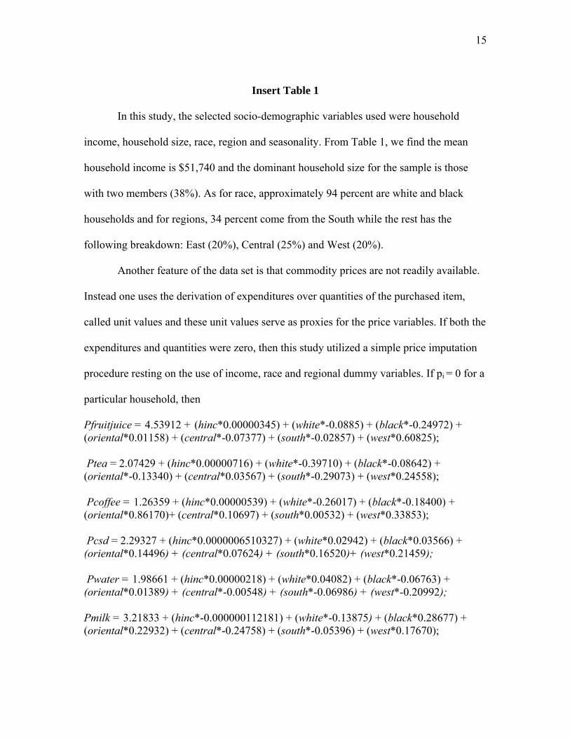
Another feature of the data set is that commodity prices are not readily available.

Instead one uses the derivation of expenditures over quantities of the purchased item,

called unit values and these unit values serve as proxies for the price variables. If both the

expenditures and quantities were zero, then this study utilized a simple price imputation

procedure resting on the use of income, race and regional dummy variables. If pi = 0 for a

particular household, then

Pfruitjuice = 4.53912 + (hinc*0.00000345) + (white*-0.0885) + (black*-0.24972) + (oriental*0.01158) + (central*-0.07377) + (south*-0.02857) + (west*0.60825); Ptea = 2.07429 + (hinc*0.00000716) + (white*-0.39710) + (black*-0.08642) + (oriental*-0.13340) + (central*0.03567) + (south*-0.29073) + (west*0.24558); Pcoffee = 1.26359 + (hinc*0.00000539) + (white*-0.26017) + (black*-0.18400) + (oriental*0.86170)+ (central*0.10697) + (south*0.00532) + (west*0.33853); Pcsd = 2.29327 + (hinc*0.0000006510327) + (white*0.02942) + (black*0.03566) + (oriental*0.14496) + (central*0.07624) + (south*0.16520)+ (west*0.21459); Pwater = 1.98661 + (hinc*0.00000218) + (white*0.04082) + (black*-0.06763) + (oriental*0.01389) + (central*-0.00548) + (south*-0.06986) + (west*-0.20992); Pmilk = 3.21833 + (hinc*-0.000000112181) + (white*-0.13875) + (black*0.28677) + (oriental*0.22932) + (central*-0.24758) + (south*-0.05396) + (west*0.17670);

16

Insert Tables 2, 3 and 4

The coefficients were derived by regressing the price of each non-alcoholic

beverage item with household income (hinc), race (white,black and oriental) and regions

(central, south and west). Tables 2, 3 and 4 present the mean total expenditures, quantity

purchased and prices for the six non-alcoholic beverages considered. In this case we find

that the top household purchases with respect to non-alcoholic beverages were

carbonated soft drinks, fruit juices, milk and coffee. The mean prices are as follows: fruit

juices ($4.71/gal), tea ($2.06/gal), coffee ($1.41/gal), carbonated soft drinks ($2.48/gal),

bottled water ($2.06/gal) and milk ($3.08/gal). On the other hand, Table 5 presents the

mean budget shares of the beverage items. For the period 1999, approximately 81 percent

of total expenditures for non alcoholic beverages are captured by carbonated soft drinks,

fruit juices and milk. The remaining 19 percent are devoted to tea (4.7 %), coffee (11%)

and bottled water (3.8 %).

Insert Table 5

Table 6 describes the degree of censoring associated with each type of non-

alcoholic beverages for each household on a quarterly basis. From the table, items with

minimal to medium censoring are milk (6.77%), carbonated soft drinks (8.84 %) and fruit

juices (23.09 %). On the other hand, the remaining highly censored non-alcoholic

beverage items are tea (54.88 %), coffee (42.77 %) and bottled water (60.65 %).

Insert Table 6

17

Empirical Results

Estimated Demand Parameters2

Almost all of the socio-demographic coefficients in both specifications and across all

estimation techniques are statistically significant. Also, almost all of the parameters in

both AIDS and QUAIDS and across estimation techniques are relatively close to one

another and the same can be said for the AIDS and QUAIDS unrestricted cases. Thus it

can be postulated that because of a relatively large sample size, the various estimation

procedures converged to yielding relatively close parameter estimates. Also, the

parameters associated with the quadratic term in the QUAIDS specification are highly

significant, suggesting in part a bias towards the QUAIDS specification over the AIDS

model across the various estimation procedures, with or without incorporating demand

restrictions. In Table 7, we find that the symmetry, homogeneity and the combination of

both restrictions are rejected in both the AIDS and QUAIDS models.

Insert Table 7

Expenditure and Compensated Elasticities

In Tables 8 to 15, we present the calculated expenditure and compensated elasticities of

non-alcoholic beverages across model specifications, estimation techniques and

imposition of theoretical restrictions. From the tables, we find that both expenditure

elasticities and own-price elasticities were generally similar across model specifications,

estimation techniques and whether or not the theoretical restrictions were imposed. All of

2 Due to space constraints, the estimated parameters are not included in the text, but are available upon request.

18

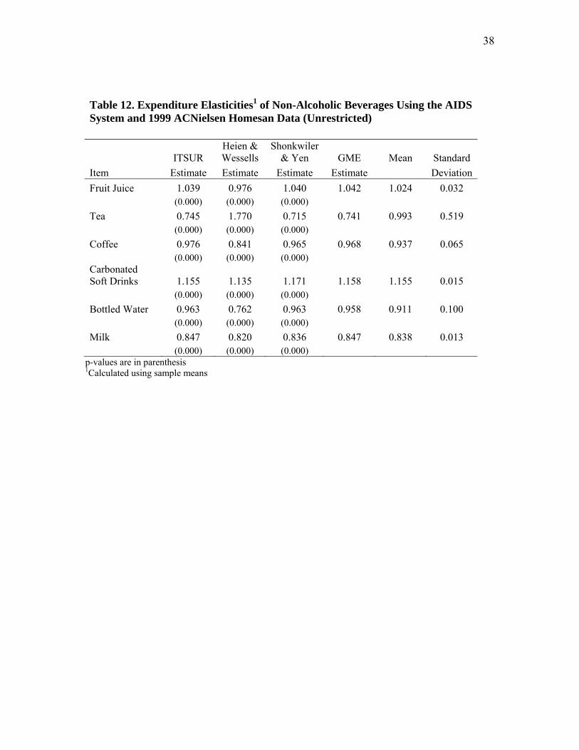
the expenditure elasticities are positive indicating that all non-alcoholic beverages are

normal goods. Also, if we look at the compensated cross-price elasticities across model

specifications, estimation techniques and with or without theoretical restrictions, we find

that almost all of them are positive indicating that the set of non-alcoholic beverages are

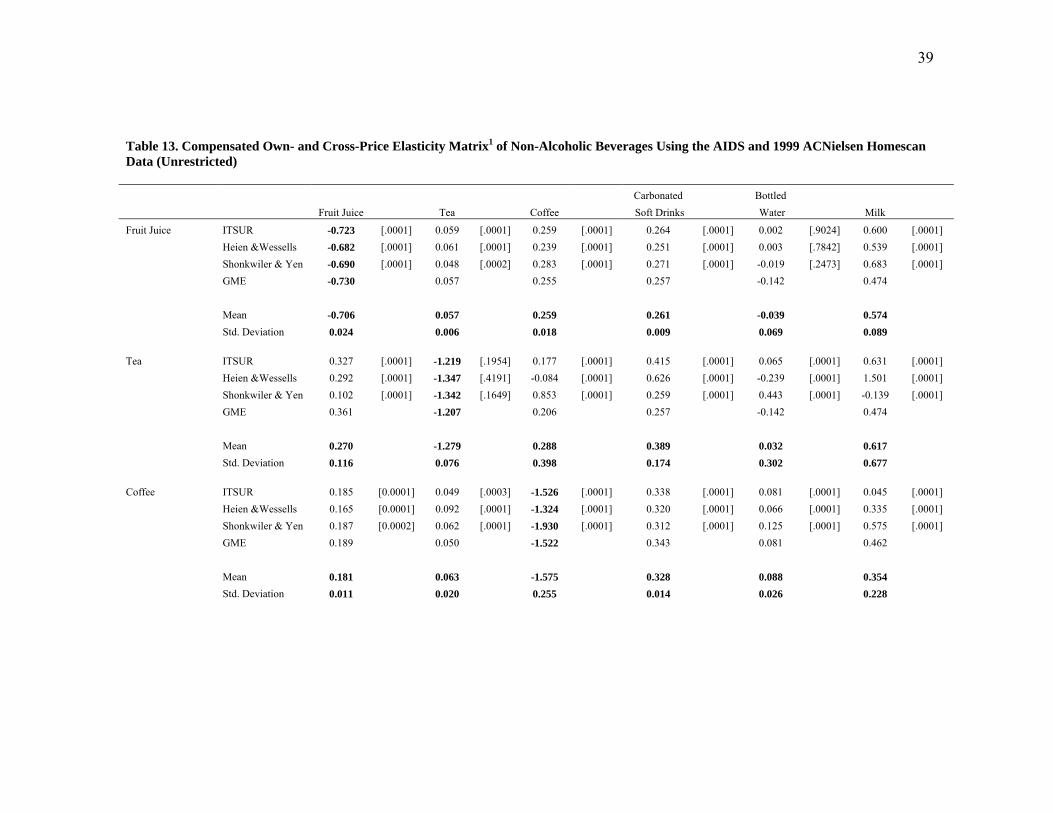
net substitutes. Similarly, the major substitutes for fruit juice and tea are coffee,

carbonated soft drink and milk. On the other hand the major substitutes for coffee are

fruit juice, carbonated soft drinks and milk. For carbonated soft drinks the major

substitutes are coffee and milk. Coffee, carbonated soft drinks and milk represent the

major non-alcoholic beverage substitutes for bottled water. Finally, the major commodity

substitutes for milk are fruit juice, coffee and carbonated soft drinks.

Insert Tables 8 to 15

Elasticity Comparisons across Censored Estimation Techniques of Non-Alcoholic

Beverages

In Table 9, we present the AIDS compensated or Hicksian price elasticity matrix of non-

alcoholic beverages. We note more variability of cross-price elasticities estimates of non-

alcoholic beverage that are highly censored, that is for tea, coffee and bottled water. On

the other hand, relatively less variable cross-price elasticity estimates were observed for

commodities with relatively fewer censoring issues. For example, in milk, the cross-price

elasticity estimates of milk with respect to fruit juice ranged from 0.152 to 0.275. The

cross-price elasticity values for bottled water with respect to fruit juice ranged from 0.011

to 0.492. Also note that associated p-values for all price elasticities are mostly significant.

For the QUAIDS specification, we note the same claim that the greater number of

19

censored observations the commodity, the more variable the respective own- and cross-

price elasticities are. For milk the compensated price elasticities with respect to fruit juice

ranged from 0.153 to 0.283, while for the bottled water, the compensated price elasticities

ranged from -0.033 to 0.451 (Table 11). On the other hand, the same observation can be

made for the AIDS and QUAIDS unrestricted cases. For example the cross-price

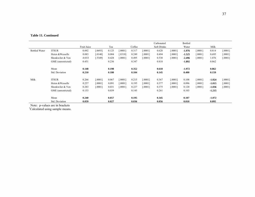
elasticity of milk with respect fruit juice ranged from 0.122 to 0.152 for AIDS (Table 13)

and 0.121 to 0.153 for QUAIDS (Table 15), while the cross-price elasticity of bottled

water with respect to fruit juice ranged from 0.372 to 0.675 for the AIDS specification

and 0.378 to 0.666 for the QUAIDS model.

Elasticity Comparisons across Model Specifications (AIDS vs. QUAIDS)

The compensated own- and cross-price elasticity matrices of non-alcoholic beverages of

both the AIDS and QUAIDS models are presented in Tables 9 and 11. We note relatively

similar price elasticity estimates especially with respect to the own-price elasticity values

of both models. For milk, the range of the AIDS own price elasticities were from -0.951

to -1.211, whereas for the QUAIDS model, the values ranged from -1.015 to -1.215. Also

if we look at a highly censored commodity such as bottled water, the cross-price

elasticity of bottled water with respect to tea ranged from 0.002 to 0.380 for the AIDS

model and 0.004 to 0.428 in the QUAIDS specification. The same findings also were

observed for the unrestricted cases of AIDS and QUAIDS where the calculated

compensated price elasticities were remarkably similar.

20

Elasticity Comparisons across Imposition of Theoretical Restrictions

In Tables 9 and 13, we show the compensated own- and cross-price elasticity matrices of

the AIDS restricted and unrestricted cases. Two notable results were observed; own-price

elasticity estimates (absolute values) were larger in the restricted case vis-à-vis the

unrestricted case. On the other hand compensated cross-price elasticities were generally

larger in absolute terms in the unrestricted case relative to the values generated in the

restricted case. The same result also was observed for the QUAIDS restricted and

unrestricted models (Tables 11 & 15).

Fit Comparisons across Econometric Techniques

Table 16 present the R-square values of the budget share equations from different

censoring econometric techniques across demand system specification and imposition of

theoretical restrictions. From the estimates, we find that across model specifications and

theoretical restrictions, the Heien and Wessells approach had the highest R-square values

in its budget share equations. On the other hand, R-square values generated by the

Shonkwiler and Yen technique registered second if theoretical restrictions are relaxed.

Likewise, the ITSUR technique placed last across demand model specifications and

theoretical impositions in terms of goodness of fit.

Insert Table 16

Conclusions

We find that the price elasticities especially the compensated price elasticities were

robust and relatively similar and statistically significant across model specifications,

estimation techniques and restriction impositions. The signs of the compensated cross-

21

price elasticities across the board were generally positive indicating that the respective

non-alcoholic beverages are net substitutes. Comparative analysis show that across

estimation techniques, greater variability of compensated cross-price elasticity estimates

were observed in highly censored non-alcoholic beverages such as tea, coffee and bottled

water. As for the comparison between model specifications (AIDS versus QUAIDS), the

compensated price estimates were remarkably similar especially for the own-price

elasticity values. Finally, the estimates for unrestricted compensated cross-price

elasticities were generally greater vis-à-vis the restricted cases. The reverse is generally

true with regard to the compensated own-price elasticity estimates. The robustness of

both the parameter estimates and the calculated expenditure and price elasticities may be

explained in part to the availability of high number of observations (n~30,000). However,

since most censored data sets do not usually have this particular characteristic, then

studies that simulate the effect of sample size will be beneficial on determining whether

robustness will still be observed for parameter estimates and price and expenditures

elasticities in the presence of differing sample sizes.

References

Arndt, C. 1999. “An Entropy Approach to Treating Binding Non-Negativity Constraints

in Demand Systems Estimation and an Application to Herbicide Demand in Corn.”

Journal of Agricultural and Resource Economics 24(1): 204-221.

Arndt, C., S. Liu and P.V. Preckel. 1999. “On Dual Approaches to Demand Systems

Estimation in the Presence of Binding Quantity Constraints.” Applied Economics

31(8), 999-1008.

Banks, J., R. Blundell and A. Lewbel. 1997. “Quadratic Engel Curves and Consumer

Demand.” The Review of Economic and Statistics 79(4): 527-539.

Deaton, A., and J. Muelbauer. 1980. “An Almost Ideal Demand System.” American

Economic Review 70(3): 312-326.

Dhar, T and J.D. Foltz. 2005. “Milk by Any Other Name Consumer Benefits from

Labeled Milk.” American Journal Agricultural Economics 87(1): 214-218.

Dong, D., B.W. Gould and H.M. Kaiser. 2004. “Food Demand in Mexico: An

Application of the Amemiya-Tobin Approach to the Estimation of a Censored Food

System.” American Journal Agricultural Economics 86(4): 1094-1107.

Golan, A., J.M Perloff and E.Z. Shen. 2001. “Estimating a Demand System with Non-

negativity Constraints: Mexican Meat Demand.” The Review of Economics and

Statistics 83(3): 541-550.

Golan, A., G. G. Judge, and D. Miller. 1996. Maximum Entropy Econometrics: Robust

Estimation with Limited Data, John Wiley & Sons.

Green, R., and J. Alston. 1990. “Elasticities in the AIDS Models.” American Journal of

Agricultural Economics 72(2): 442-445.

Greene, W.T. 2008. Econometric Analysis. 6th Edition. Upper Saddle River, New Jersey:

Prentice Hall.

Heien, D. and C.R. Wessells. 1990. “Demand Systems Estimation with Microdata: A

Censored Regression Approach.” Journal of Business and Economic Statistics 8(3):

365-371.

Meyerhoefer, C., C.K. Ranney and D.E. Sahn. 2005. “Consistent Estimation of Censored

Demand Systems using Panel Data.” American Journal Agricultural Economics

87(3): 660-672.

Mutuc, M.E., S. Pan, and R.M. Rejesus. 2007. “Household Vegetable Demand in the

Philippines: Is There an Urban-Rural Divide.” Agribusiness: An International Journal

23(4): 511-527.

SAS Institute Inc. 2008. SAS/ETS ® 9.2 User’s Guide. Cary, North Carolina: SAS

Institute Inc.

Shonkwiler, J.S. and S.T. Yen. 1999. “Two-Step Estimation of a Censored System of

Equations.” American Journal of Agricultural Economics 81(4): 972-982.

Stockton, M.C., O. Capps, Jr and D. Dong. 2007. “A Micro Level Demand Analysis of

Selected Non-Alcoholic Beverages with Emphasis on Container Size.” Department of

Agricultural Economics, Texas A&M University, Research Report.

Tiffin, R., and M. Aquiar. 1995. “Bayesian Estimation of an Almost Ideal Demand

System for Fresh Fruit in Portugal.” European Review of Agriculture Economics

22(4): 469-80

Yen, S.T., B. Lin, and D.M. Smallwood. 2003. "Quasi and Simulated Likelihood

Approaches to Censored Demand Systems: Food Consumption by Food Stamp

Recipients in the United States." American Journal of Agricultural Economics 85(2):

458-478.

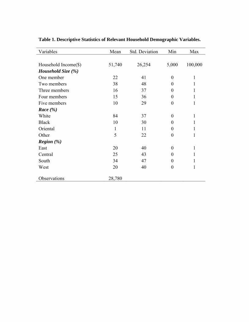
Table 1. Descriptive Statistics of Relevant Household Demographic Variables. Variables Mean Std. Deviation Min Max Household Income($) 51,740 26,254 5,000 100,000 Household Size (%) One member 22 41 0 1 Two members 38 48 0 1 Three members 16 37 0 1 Four members 15 36 0 1 Five members 10 29 0 1 Race (%) White 84 37 0 1 Black 10 30 0 1 Oriental 1 11 0 1 Other 5 22 0 1 Region (%) East 20 40 0 1 Central 25 43 0 1 South 34 47 0 1 West 20 40 0 1 Observations 28,780

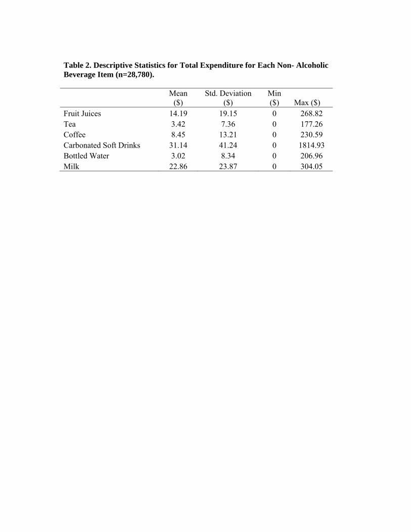
Table 2. Descriptive Statistics for Total Expenditure for Each Non- Alcoholic Beverage Item (n=28,780).

Mean

($) Std. Deviation

($) Min ($) Max ($)

Fruit Juices 14.19 19.15 0 268.82 Tea 3.42 7.36 0 177.26 Coffee 8.45 13.21 0 230.59 Carbonated Soft Drinks 31.14 41.24 0 1814.93 Bottled Water 3.02 8.34 0 206.96 Milk 22.86 23.87 0 304.05

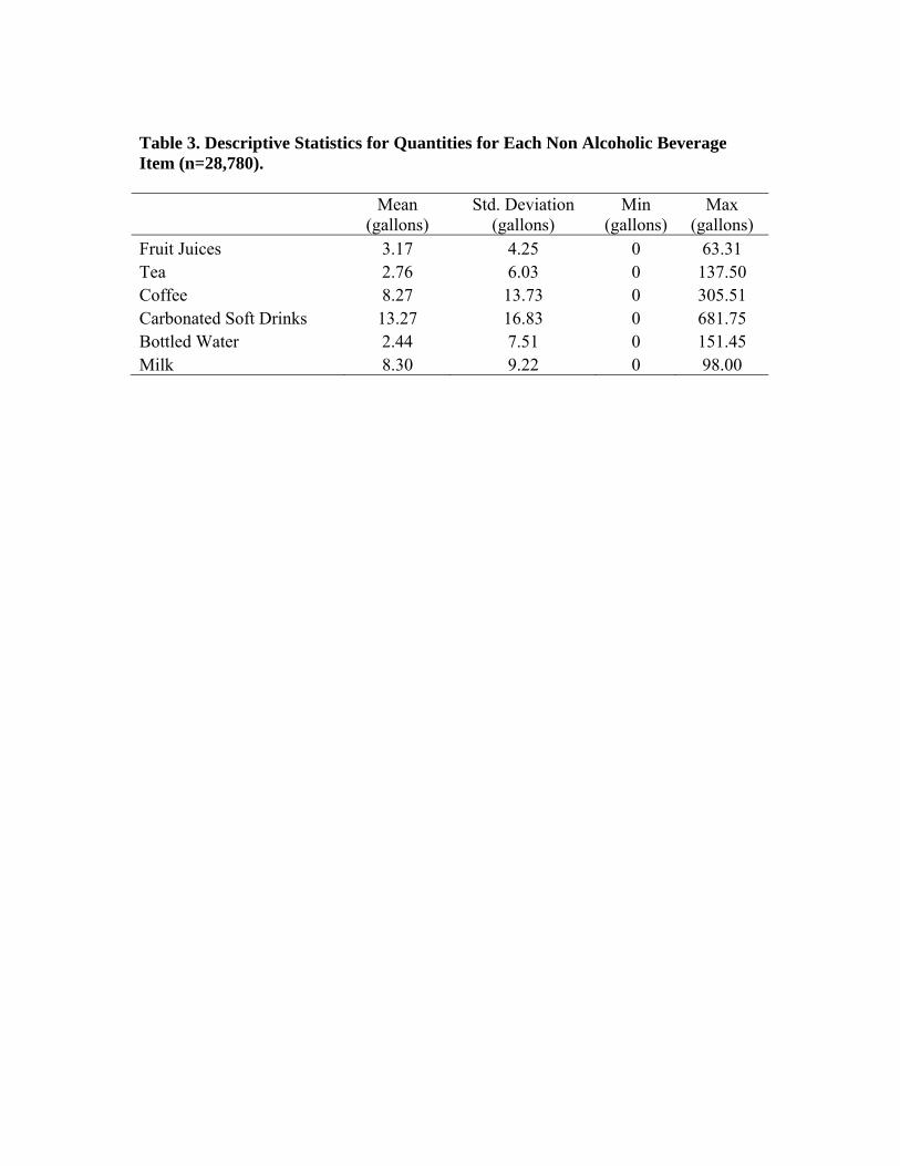
Table 3. Descriptive Statistics for Quantities for Each Non Alcoholic Beverage Item (n=28,780).

Mean

(gallons) Std. Deviation

(gallons) Min

(gallons) Max

(gallons) Fruit Juices 3.17 4.25 0 63.31 Tea 2.76 6.03 0 137.50 Coffee 8.27 13.73 0 305.51 Carbonated Soft Drinks 13.27 16.83 0 681.75 Bottled Water 2.44 7.51 0 151.45 Milk 8.30 9.22 0 98.00

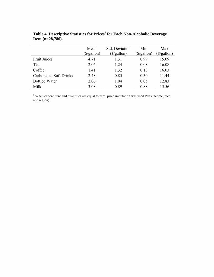
Table 4. Descriptive Statistics for Prices1 for Each Non-Alcoholic Beverage Item (n=28,780).

Mean

($/gallon) Std. Deviation

($/gallon) Min

($/gallon) Max

($/gallon)Fruit Juices 4.71 1.31 0.99 15.09 Tea 2.06 1.24 0.08 16.08 Coffee 1.41 1.32 0.13 16.03 Carbonated Soft Drinks 2.48 0.85 0.30 11.44 Bottled Water 2.06 1.04 0.05 12.83 Milk 3.08 0.89 0.88 15.56

1 When expenditure and quantities are equal to zero, price imputation was used Pi=f (income, race and region).

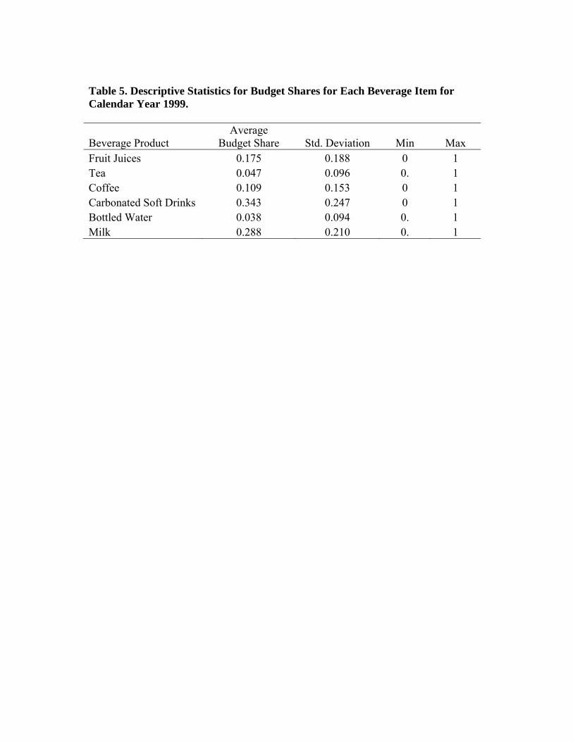
Table 5. Descriptive Statistics for Budget Shares for Each Beverage Item for Calendar Year 1999.

Beverage Product Average

Budget Share Std. Deviation Min Max Fruit Juices 0.175 0.188 0 1 Tea 0.047 0.096 0. 1 Coffee 0.109 0.153 0 1 Carbonated Soft Drinks 0.343 0.247 0 1 Bottled Water 0.038 0.094 0. 1 Milk 0.288 0.210 0. 1

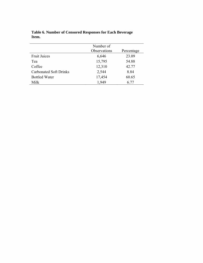
Table 6. Number of Censored Responses for Each Beverage Item.

Number of

Observations Percentage Fruit Juices 6,646 23.09 Tea 15,795 54.88 Coffee 12,310 42.77 Carbonated Soft Drinks 2,544 8.84 Bottled Water 17,454 60.65 Milk 1,949 6.77

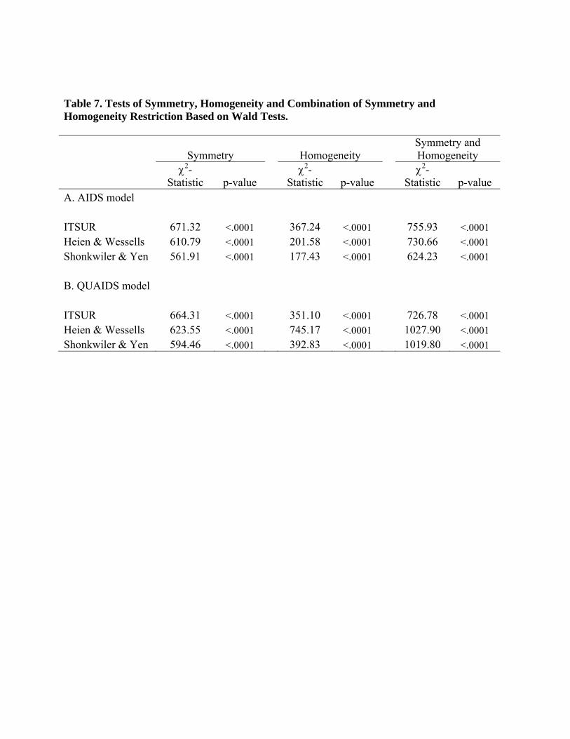
Table 7. Tests of Symmetry, Homogeneity and Combination of Symmetry and Homogeneity Restriction Based on Wald Tests.

Symmetry Homogeneity Symmetry and Homogeneity

χ2-

Statistic p-value χ2-

Statistic p-value χ2-

Statistic p-value A. AIDS model ITSUR 671.32 <.0001 367.24 <.0001 755.93 <.0001 Heien & Wessells 610.79 <.0001 201.58 <.0001 730.66 <.0001 Shonkwiler & Yen 561.91 <.0001 177.43 <.0001 624.23 <.0001 B. QUAIDS model ITSUR 664.31 <.0001 351.10 <.0001 726.78 <.0001 Heien & Wessells 623.55 <.0001 745.17 <.0001 1027.90 <.0001 Shonkwiler & Yen 594.46 <.0001 392.83 <.0001 1019.80 <.0001

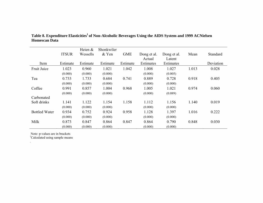
Table 8. Expenditure Elasticities1 of Non-Alcoholic Beverages Using the AIDS System and 1999 ACNielsen Homescan Data

ITSUR Heien & Wessells

Shonkwiler & Yen GME Dong et al. Dong et al. Mean Standard

Item Estimate Estimate Estimate Estimate Actual

Estimates Latent

Estimates Deviation Fruit Juice 1.023 0.960 1.021 1.042 1.008 1.027 1.013 0.028 (0.000) (0.000) (0.000) (0.000) (0.005)

Tea 0.733 1.733 0.684 0.741 0.889 0.728 0.918 0.405 (0.000) (0.000) (0.000) (0.000) (0.000)

Coffee 0.991 0.857 1.004 0.968 1.005 1.021 0.974 0.060 (0.000) (0.000) (0.000) (0.000) (0.089) Carbonated Soft drinks 1.141 1.122 1.154 1.158 1.112 1.156 1.140 0.019 (0.000) (0.000) (0.000) (0.000) (0.000)

Bottled Water 0.934 0.752 0.924 0.958 1.128 1.397 1.016 0.222 (0.000) (0.000) (0.000) (0.000) (0.000)

Milk 0.873 0.847 0.864 0.847 0.864 0.790 0.848 0.030 (0.000) (0.000) (0.000) (0.000) (0.000)

Note: p-values are in brackets 1Calculated using sample means .

Table 9. Compensated Own- and Cross-Price Elasticity Matrix1 of Non-Alcoholic Beverages Using the AIDS and the 1999 ACNielsen Homescan Data

Fruit Carbonated Bottled Juice Tea Coffee Soft Drinks Water Milk Fruit Juice ITSUR -0.827 [.0001] 0.050 [.0001] 0.193 [.0001] 0.139 [.0001] 0.020 [.0108] 0.425 [.0001] Heien &Wessells -0.777 [.0001] 0.040 [.0001] 0.173 [.0001] 0.139 [.0001] 0.018 [.0149] 0.407 [.0001] Shonkwiler & Yen -0.812 [.0001] 0.022 [.0245] 0.231 [.0001] 0.114 [.0001] 0.001 [.9528] 0.445 [.0001] Dong et. al (actual) -0.877 [.0001] 0.064 [0.0001] 0.189 [.0001] 0.202 [.0001] -0.006 [.1923] 0.428 [.0001] Dong e.t al (latent) -0.913 0.091 0.265 0.065 -0.006 0.498 GME(unrestricted) -0.730 0.057 0.255 0.257 -0.142 0.474 Mean -0.823 0.054 0.218 0.153 -0.019 0.446 Std. Deviation 0.066 0.023 0.038 0.068 0.061 0.034 Tea ITSUR 0.199 [.0001] -1.244 [.0001] 0.153 [.0001] 0.399 [.0001] 0.103 [.0001] 0.390 [.0001] Heien &Wessells 0.115 [.0001] -1.224 [.0001] 0.011 [.5905] 0.530 [.0001] -0.016 [.2609] 0.585 [.0001] Shonkwiler & Yen 0.101 [.0073] -1.496 [.0001] 0.587 [.0001] 0.373 [.0001] 0.296 [.0001] 0.139 [.0001] Dong et al (actual) 0.190 [.0001] -1.256 [0.0001] 0.147 [.0001] 0.425 [.0001] 0.051 [.0001] 0.442 [.0001] Dong et al (latent) 0.210 -1.725 0.216 0.519 0.135 0.645 GME (unrestricted) 0.361 -1.207 0.206 0.257 -0.142 0.474 Mean 0.196 -1.359 0.220 0.417 0.071 0.446 Std. Deviation 0.093 0.209 0.194 0.101 0.148 0.177 Coffee ITSUR 0.310 [0.0001] 0.066 [.0001] -1.483 [.0001] 0.437 [.0001] 0.109 [.0001] 0.560 [.0001] Heien &Wessells 0.284 [0.0001] 0.008 [.3918] -1.270 [.0001] 0.393 [.0001] 0.090 [.0001] 0.495 [.0001] Shonkwiler & Yen 0.376 [0.0001] 0.231 [.0001] -1.764 [.0001] 0.442 [.0001] 0.193 [.0001] 0.522 [.0001] Dong et. al (actual) 0.289 [.0001] 0.061 [.0001] -1.337 [.0001] 0.437 [.0001] 0.092 [.0001] 0.459 [.0001] Dong et. al (latent) 0.409 0.090 -1.785 0.500 0.192 0.594 GME (unrestricted) 0.189 0.050 -1.522 0.343 0.081 0.462 Mean 0.310 0.084 -1.527 0.425 0.126 0.515 Std. Deviation 0.077 0.077 0.213 0.053 0.052 0.054

Table 9. Continued Fruit Carbonated Bottled Juice Tea Coffee Soft Drinks Water Milk Carbonated Soft drinks ITSUR 0.064 [.0001] 0.054 [.0001] 0.139 [.0001] -0.645 [.0001] 0.068 [.0001] 0.320 [.0001] Heien &Wessells 0.066 [.0001] 0.069 [.0001] 0.125 [.0001] -0.642 [.0001] 0.053 [.0001] 0.329 [.0001] Shonkwiler & Yen 0.049 [.0001] 0.054 [.0001] 0.115 [.0001] -0.637 [.0001] 0.067 [.0001] 0.352 [.0001] Dong et al (actual) 0.112 [.0001] 0.067 [.0001] 0.137 [.0001] -0.676 [.0001] 0.084 [.0001] 0.276 [.0001] Dong et al (latent) 0.096 0.093 0.181 [.0001] -0.708 0.132 0.207 GME (unrestricted) 0.080 0.071 0.160 -0.603 0.091 0.377 Mean 0.078 0.068 0.143 -0.652 0.083 0.310 Std. Deviation 0.023 0.014 0.024 0.036 0.028 0.061 Bottled Water ITSUR 0.097 [.0089] 0.125 [.0001] 0.314 [.0001] 0.628 [.0001] -1.977 [.0001] 0.814 [.0001] Heien &Wessells 0.088 [.0090] 0.002 [.8978] 0.250 [.0001] 0.493 [.0001] -1.527 [.0001] 0.694 [.0001] Shonkwiler & Yen 0.011 [.8326] 0.351 [.0001] 0.566 [.0001] 0.651 [.0001] -2.541 [.0001] 0.962 [.0001] Dong et al (actual) 0.139 [.0001] 0.146 [.0001] 0.278 [.0001] 0.512 [.0001] -1.807 [.0001] 0.732 [.0001] Dong et al (latent) 0.068 0.380 0.670 0.811 -3.455 1.525 GME (unrestricted) 0.492 0.225 0.389 0.791 -1.908 0.853 Mean 0.149 0.205 0.411 0.648 -2.203 0.930 Std. Deviation 0.173 0.144 0.170 0.134 0.698 0.307 Milk ITSUR 0.264 [.0001] 0.067 [.0001] 0.213 [.0001] 0.370 [.0001] 0.109 [.0001] -1.023 [.0001] Heien &Wessells 0.256 [.0001] 0.090 [.0001] 0.192 [.0001] 0.380 [.0001] 0.097 [.0001] -1.014 [.0001] Shonkwiler & Yen 0.275 [.0001] 0.032 [.0001] 0.219 [.0001] 0.375 [.0001] 0.134 [.0001] -1.036 [.0001] Dong et al (actual) 0.235 [.0001] 0.052 [.0001] 0.195 [.0001] 0.381 [.0001] 0.088 [.0001] -0.951 [.0001] Dong et al (latent) 0.272 0.074 0.281 0.383 0.152 -1.162 GME (unrestricted) 0.152 0.040 0.148 0.251 0.102 -1.211 Mean 0.242 0.059 0.208 0.357 0.114 -1.066 Std. Deviation 0.046 0.022 0.044 0.052 0.024 0.099

Note: p-values are in brackets 1Calculated using sample means.

35

Table 10. Expenditure Elasticities1 of Non-Alcoholic Beverages Using the QUAIDS System and 1999 ACNielsen Homescan Data

ITSUR Heien & Wessells

Shonkwiler & Yen GME Mean Standard

Item Estimate Estimate Estimate Estimate DeviationFruit Juice 0.982 0.932 0.964 1.010 0.972 0.033 (0.000) (0.000) (0.000) Tea 0.767 1.601 0.841 0.776 0.996 0.404 (0.000) (0.000) (0.000) Coffee 0.879 0.757 0.844 0.872 0.838 0.056 (0.000) (0.000) (0.000) Carbonated Soft drinks 1.184 1.171 1.189 1.201 1.186 0.012 (0.000) (0.000) (0.000) Bottled Water 1.033 0.828 1.127 1.054 1.011 0.128 (0.000) (0.000) (0.000) Milk 0.870 0.855 0.864 0.833 0.856 0.016 (0.000) (0.000) (0.000)

Note: p-values are in brackets 1Calculated using sample means

36

Table 11. Compensated Own- and Cross-Price Elasticity Matrix1 of Non-Alcoholic Beverages Using the QUAIDS and the 1999 ACNielsen Homescan Data

Carbonated Bottled Fruit Juice Tea Coffee Soft Drinks Water Milk Fruit Juice ITSUR -0.826 [.0001] 0.050 [.0001] 0.191 [.0001] 0.140 [.0001] 0.020 [.0108] 0.426 [.0001] Heien &Wessells -0.776 [.0001] 0.040 [.0001] 0.172 [.0001] 0.139 [.0001] 0.018 [.0214] 0.408 [.0001] Shonkwiler & Yen -0.805 [.0001] 0.013 [.2032] 0.247 [.0001] 0.117 [.0001] -0.009 [.4151] 0.438 [.0001] GME (unrestricted) -0.716 0.043 0.270 0.251 -0.172 0.469 Mean -0.781 0.036 0.220 0.162 -0.036 0.435 Std. Deviation 0.048 0.016 0.046 0.060 0.092 0.026 Tea ITSUR 0.197 [.0001] -1.243 [.0001] 0.154 [.0001] 0.399 [.0001] 0.103 [.0001] 0.391 [.0001] Heien &Wessells 0.115 [.0001] -1.228 [.0001] -0.002 [.9184] 0.544 [.0001] -0.011 [.4564] 0.581 [.0001] Shonkwiler & Yen 0.067 [.0772] -1.422 [.0001] 0.480 [.0001] 0.365 [.0001] 0.321 [.0001] 0.189 [.0001] GME (unrestricted) 0.337 -1.199 0.175 0.482 0.078 0.737 Mean 0.179 -1.273 0.202 0.447 0.123 0.475 Std. Deviation 0.118 0.101 0.202 0.081 0.141 0.237 Coffee ITSUR 0.313 [0.0001] 0.066 [.0001] -1.490 [.0001] 0.442 [.0001] 0.111 [.0001] 0.558 [.0001] Heien &Wessells 0.286 [0.0001] 0.006 [.5303] -1.275 [.0001] 0.397 [.0001] 0.091 [.0001] 0.495 [.0001] Shonkwiler & Yen 0.396 [0.0001] 0.182 [.0001] -1.700 [.0001] 0.487 [.0001] 0.164 [.0001] 0.471 [.0001] GME (unrestricted) 0.228 0.039 -1.484 0.336 0.068 0.452 Mean 0.306 0.073 -1.487 0.415 0.108 0.494 Std. Deviation 0.070 0.077 0.174 0.065 0.041 0.046 Carbonated ITSUR 0.062 [.0001] 0.054 [.0001] 0.139 [.0001] -0.644 [.0001] 0.068 [.0001] 0.321 [.0001] Soft drinks Heien &Wessells 0.064 [.0001] 0.069 [.0001] 0.126 [.0001] -0.642 [.0001] 0.052 [.0001] 0.331 [.0001] Shonkwiler & Yen 0.042 [.0001] 0.057 [.0001] 0.103 [.0001] -0.638 [.0001] 0.084 [.0001] 0.352 [.0001] GME (unrestricted) 0.067 0.073 0.152 -0.611 0.094 0.384 Mean 0.059 0.064 0.130 -0.634 0.075 0.347 Std. Deviation 0.011 0.009 0.021 0.016 0.019 0.028

37

Table 11. Continued Carbonated Bottled Fruit Juice Tea Coffee Soft Drinks Water Milk Bottled Water ITSUR 0.092 [.0693] 0.125 [.0001] 0.317 [.0001] 0.628 [.0001] -1.976 [.0001] 0.814 [.0001] Heien &Wessells 0.083 [.0140] 0.004 [.8310] 0.249 [.0001] 0.494 [.0001] -1.525 [.0001] 0.695 [.0001] Shonkwiler & Yen -0.033 [.5349] 0.428 [.0001] 0.495 [.0001] 0.530 [.0001] -2.496 [.0001] 1.076 [.0001] GME (unrestricted) 0.451 0.236 0.347 0.818 -1.892 0.862 Mean 0.148 0.198 0.352 0.618 -1.972 0.862 Std. Deviation 0.210 0.180 0.104 0.145 0.400 0.159 Milk ITSUR 0.266 [.0001] 0.067 [.0001] 0.215 [.0001] 0.367 [.0001] 0.108 [.0001] -1.024 [.0001] Heien &Wessells 0.257 [.0001] 0.091 [.0001] 0.195 [.0001] 0.377 [.0001] 0.096 [.0001] -1.015 [.0001] Shonkwiler & Yen 0.283 [.0001] 0.031 [.0001] 0.227 [.0001] 0.375 [.0001] 0.120 [.0001] -1.036 [.0001] GME (unrestricted) 0.153 0.039 0.145 0.261 0.103 -1.215 Mean 0.240 0.057 0.195 0.345 0.107 -1.072 Std. Deviation 0.059 0.027 0.036 0.056 0.010 0.095 Note: p-values are in brackets

1Calculated using sample means.

38

Table 12. Expenditure Elasticities1 of Non-Alcoholic Beverages Using the AIDS System and 1999 ACNielsen Homesan Data (Unrestricted)

ITSUR Heien & Wessells

Shonkwiler & Yen GME Mean Standard

Item Estimate Estimate Estimate Estimate DeviationFruit Juice 1.039 0.976 1.040 1.042 1.024 0.032 (0.000) (0.000) (0.000) Tea 0.745 1.770 0.715 0.741 0.993 0.519 (0.000) (0.000) (0.000) Coffee 0.976 0.841 0.965 0.968 0.937 0.065 (0.000) (0.000) (0.000) Carbonated Soft Drinks 1.155 1.135 1.171 1.158 1.155 0.015 (0.000) (0.000) (0.000) Bottled Water 0.963 0.762 0.963 0.958 0.911 0.100 (0.000) (0.000) (0.000) Milk 0.847 0.820 0.836 0.847 0.838 0.013 (0.000) (0.000) (0.000)

p-values are in parenthesis 1Calculated using sample means

39

Table 13. Compensated Own- and Cross-Price Elasticity Matrix1 of Non-Alcoholic Beverages Using the AIDS and 1999 ACNielsen Homescan Data (Unrestricted)

Carbonated Bottled Fruit Juice Tea Coffee Soft Drinks Water Milk Fruit Juice ITSUR -0.723 [.0001] 0.059 [.0001] 0.259 [.0001] 0.264 [.0001] 0.002 [.9024] 0.600 [.0001] Heien &Wessells -0.682 [.0001] 0.061 [.0001] 0.239 [.0001] 0.251 [.0001] 0.003 [.7842] 0.539 [.0001] Shonkwiler & Yen -0.690 [.0001] 0.048 [.0002] 0.283 [.0001] 0.271 [.0001] -0.019 [.2473] 0.683 [.0001] GME -0.730 0.057 0.255 0.257 -0.142 0.474 Mean -0.706 0.057 0.259 0.261 -0.039 0.574 Std. Deviation 0.024 0.006 0.018 0.009 0.069 0.089 Tea ITSUR 0.327 [.0001] -1.219 [.1954] 0.177 [.0001] 0.415 [.0001] 0.065 [.0001] 0.631 [.0001] Heien &Wessells 0.292 [.0001] -1.347 [.4191] -0.084 [.0001] 0.626 [.0001] -0.239 [.0001] 1.501 [.0001] Shonkwiler & Yen 0.102 [.0001] -1.342 [.1649] 0.853 [.0001] 0.259 [.0001] 0.443 [.0001] -0.139 [.0001] GME 0.361 -1.207 0.206 0.257 -0.142 0.474 Mean 0.270 -1.279 0.288 0.389 0.032 0.617 Std. Deviation 0.116 0.076 0.398 0.174 0.302 0.677 Coffee ITSUR 0.185 [0.0001] 0.049 [.0003] -1.526 [.0001] 0.338 [.0001] 0.081 [.0001] 0.045 [.0001] Heien &Wessells 0.165 [0.0001] 0.092 [.0001] -1.324 [.0001] 0.320 [.0001] 0.066 [.0001] 0.335 [.0001] Shonkwiler & Yen 0.187 [0.0002] 0.062 [.0001] -1.930 [.0001] 0.312 [.0001] 0.125 [.0001] 0.575 [.0001] GME 0.189 0.050 -1.522 0.343 0.081 0.462 Mean 0.181 0.063 -1.575 0.328 0.088 0.354 Std. Deviation 0.011 0.020 0.255 0.014 0.026 0.228

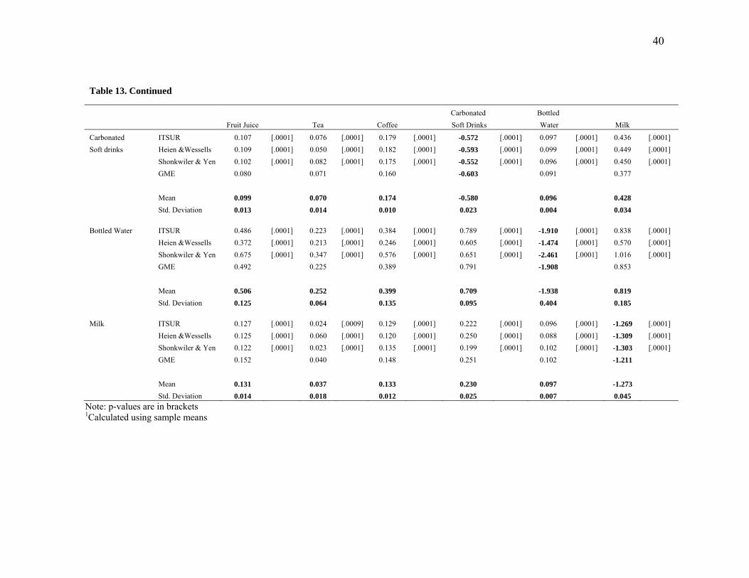
40

Table 13. Continued Carbonated Bottled Fruit Juice Tea Coffee Soft Drinks Water Milk Carbonated ITSUR 0.107 [.0001] 0.076 [.0001] 0.179 [.0001] -0.572 [.0001] 0.097 [.0001] 0.436 [.0001] Soft drinks Heien &Wessells 0.109 [.0001] 0.050 [.0001] 0.182 [.0001] -0.593 [.0001] 0.099 [.0001] 0.449 [.0001] Shonkwiler & Yen 0.102 [.0001] 0.082 [.0001] 0.175 [.0001] -0.552 [.0001] 0.096 [.0001] 0.450 [.0001] GME 0.080 0.071 0.160 -0.603 0.091 0.377 Mean 0.099 0.070 0.174 -0.580 0.096 0.428 Std. Deviation 0.013 0.014 0.010 0.023 0.004 0.034 Bottled Water ITSUR 0.486 [.0001] 0.223 [.0001] 0.384 [.0001] 0.789 [.0001] -1.910 [.0001] 0.838 [.0001] Heien &Wessells 0.372 [.0001] 0.213 [.0001] 0.246 [.0001] 0.605 [.0001] -1.474 [.0001] 0.570 [.0001] Shonkwiler & Yen 0.675 [.0001] 0.347 [.0001] 0.576 [.0001] 0.651 [.0001] -2.461 [.0001] 1.016 [.0001] GME 0.492 0.225 0.389 0.791 -1.908 0.853 Mean 0.506 0.252 0.399 0.709 -1.938 0.819 Std. Deviation 0.125 0.064 0.135 0.095 0.404 0.185 Milk ITSUR 0.127 [.0001] 0.024 [.0009] 0.129 [.0001] 0.222 [.0001] 0.096 [.0001] -1.269 [.0001] Heien &Wessells 0.125 [.0001] 0.060 [.0001] 0.120 [.0001] 0.250 [.0001] 0.088 [.0001] -1.309 [.0001] Shonkwiler & Yen 0.122 [.0001] 0.023 [.0001] 0.135 [.0001] 0.199 [.0001] 0.102 [.0001] -1.303 [.0001] GME 0.152 0.040 0.148 0.251 0.102 -1.211 Mean 0.131 0.037 0.133 0.230 0.097 -1.273 Std. Deviation 0.014 0.018 0.012 0.025 0.007 0.045

Note: p-values are in brackets 1Calculated using sample means

41

Table 14. Expenditure Elasticities1 of Non-Alcoholic Beverages Using the QUAIDS System and 1999 ACNielsen Homescan Data (Unrestricted)

ITSUR Heien & Wessells

Shonkwiler & Yen GME Mean Standard

Item Estimate Estimate Estimate Estimate Deviation Fruit Juice 1.054 0.956 1.079 1.010 1.025 0.054 (0.000) (0.000) (0.000) Tea 0.586 1.547 0.929 0.776 0.959 0.416 (0.000) (0.000) (0.000) Coffee 0.988 0.734 0.661 0.872 0.814 0.145 (0.000) (0.000) (0.000) Carbonated Soft Drinks 1.162 1.198 1.199 1.201 1.190 0.019 (0.000) (0.000) (0.000) Bottled Water 0.943 0.862 0.995 1.054 0.963 0.081 (0.000) (0.000) (0.000) Milk 0.854 0.820 0.856 0.833 0.841 0.017 (0.000) (0.000) (0.000)

Note: p-values are in brackets 1Calculated using sample means

42

Table 15. Compensated Own- and Cross-Price Elasticity Matrix1 of Non-Alcoholic Beverages Using the QUAIDS and the 1999 ACNielsen Homescan Data (Unrestricted)

Carbonated Bottled Fruit Juice Tea Coffee Soft Drinks Water Milk Fruit Juice ITSUR -0.723 [.0001] 0.100 [.0001] 0.258 [.0001] 0.268 [.0001] 0.003 [.8061] 0.600 [.0001] Heien &Wessells -0.683 [.0001] 0.017 [.3264] 0.238 [.0001] 0.246 [.0001] 0.003 [.8260] 0.539 [.0001] Shonkwiler & Yen -0.698 [.0001] 0.071 [.0001] 0.502 [.0001] 0.275 [.0001] 0.003 [.8804] 0.687 [.0001] GME -0.716 0.043 0.270 0.251 -0.172 0.469 Mean -0.705 0.058 0.317 0.260 -0.041 0.574 Std. Deviation 0.018 0.036 0.124 0.014 0.087 0.093 Tea ITSUR 0.312 [.0001] -1.658 [.0001] 0.179 [.0001] 0.361 [.0001] 0.037 [.0001] 0.622 [.0001] Heien &Wessells 0.276 [.0001] -1.207 [.0001] -0.119 [.0001] 0.671 [.0001] -0.254 [.0001] 1.424 [.0001] Shonkwiler & Yen 0.089 [.0001] -1.383 [.0001] 2.085 [.0001] 0.390 [.0001] 0.555 [.0001] -0.184 [.0001] GME 0.337 -1.199 0.175 0.482 0.078 0.737 Mean 0.254 -1.362 0.580 0.476 0.104 0.650 Std. Deviation 0.113 0.215 1.013 0.140 0.335 0.659 Coffee ITSUR 0.185 [0.0001] 0.081 [.0001] -1.527 [.0001] 0.342 [.0001] 0.083 [.0001] 0.454 [.0001] Heien &Wessells 0.163 [0.0001] -0.163 [.0001] -1.330 [.0001] 0.304 [.0001] 0.070 [.0001] 0.351 [.0001] Shonkwiler & Yen 0.240 [0.0001] -0.052 [.1667] -3.728 [.0001] 0.227 [.0001] -0.042 [.2921] 0.580 [.0001] GME 0.228 0.039 -1.484 0.336 0.068 0.452 Mean 0.204 -0.024 -2.017 0.302 0.044 0.459 Std. Deviation 0.036 0.108 1.144 0.053 0.058 0.094 Carbonated Soft drinks ITSUR 0.106 [.0001] 0.096 [.0001] 0.178 [.0001] -0.572 [.0001] 0.098 [.0001] 0.438 [.0001] Heien &Wessells 0.110 [.0001] 0.214 [.0001] 0.184 [.0001] -0.578 [.0001] 0.097 [.0001] 0.435 [.0001] Shonkwiler & Yen 0.093 [.0001] 0.108 [.0001] 0.348 [.0001] -0.561 [.0001] 0.112 [.0001] 0.461 [.0001] GME 0.067 0.073 0.152 -0.611 0.094 0.384 Mean 0.094 0.123 0.216 -0.580 0.100 0.429 Std. Deviation 0.019 0.062 0.089 0.021 0.008 0.033

43

Table 15. Continued Carbonated Bottled Fruit Juice Tea Coffee Soft Drinks Water Milk Bottled Water ITSUR 0.486 [.0001] 0.167 [.0001] 0.385 [.0001] 0.783 [.0001] -1.912 [.0001] 0.837 [.0001] Heien &Wessells 0.378 [.0001] 0.358 [.0001] 0.261 [.0001] 0.593 [.0001] -1.467 [.0001] 0.602 [.0001] Shonkwiler & Yen 0.666 [.0001] 0.354 [.0001] 0.819 [.0001] 1.029 [.0001] -2.440 [.0001] 1.180 [.0001] GME 0.451 0.236 0.347 0.818 -1.892 0.862 Mean 0.495 0.279 0.453 0.806 -1.928 0.870 Std. Deviation 0.122 0.093 0.250 0.179 0.399 0.237 Milk ITSUR 0.128 [.0001] 0.043 [.0001] 0.129 [.0001] 0.227 [.0001] 0.096 [.0001] -1.270 [.0001] Heien &Wessells 0.127 [.0001] 0.022 [.0594] 0.124 [.0001] 0.236 [.0001] 0.091 [.0001] -1.290 [.0001] Shonkwiler & Yen 0.121 [.0001] 0.026 [.0001] 0.243 [.0001] 0.216 [.0001] 0.112 [.0001] -1.311 [.0001] GME 0.153 0.039 0.145 0.261 0.103 -1.215 Mean 0.132 0.033 0.160 0.235 0.101 -1.271 Std. Deviation 0.014 0.010 0.056 0.019 0.009 0.041

Note: p-values are in brackets 1Calculated using sample means

44

Table 16. R-squared Values of Budget Share Equations from Different Censoring Econometric Techniques. Micro-Demand Econometric Fruit Juice Coffee Soft Drink Bottled Water Milk Tea System Model Techniques w_f w_c w_s w_w w_m w_t AIDS ITSUR 0.0622 0.0673 0.0484 0.0764 0.0734 0.0184 Heien & Wessells 0.1937 0.3202 0.0966 0.2593 0.1441 0.0038 Shonkwiler & Yen 0.0629 0.0641 0.0479 0.0720 0.0744 0.0133 GME (unrestricted) 0.0673 0.0695 0.0537 0.0801 0.0937 0.0145 Dong et. al 0.0139 0.0484 0.0016 0.0676 0.0253 0.0101 QUAIDS ITSUR 0.0636 0.0732 0.0517 0.0779 0.0734 0.0189 Heien & Wessells 0.1956 0.3259 0.1054 0.2602 0.1463 0.0037 Shonkwiler & Yen 0.0643 0.0702 0.0511 0.0740 0.0742 0.0155 GME (unrestricted) 0.0681 0.0742 0.0571 0.0816 0.0940 0.0150 AIDS ITSUR 0.0672 0.0694 0.0532 0.0801 0.0940 0.0035 (unrestricted) Heien & Wessells 0.1981 0.3257 0.1008 0.2649 0.1699 0.0113 Shonkwiler & Yen 0.0676 0.0697 0.0529 0.0766 0.0944 0.0005 GME 0.0673 0.0695 0.0537 0.0801 0.0937 0.0145 QUAIDS ITSUR 0.0682 0.0697 0.0536 0.0804 0.0946 0.0030 (unrestricted) Heien & Wessells 0.1995 0.3299 0.1106 0.2656 0.1721 0.0001 Shonkwiler & Yen 0.0696 0.1076 0.0562 0.0768 0.0958 0.0037 GME 0.0681 0.0742 0.0571 0.0816 0.0940 0.0150