lecture 16: markov chain monte carlo(contd)STAT 545: Intro. to Computational Statistics

Vinayak RaoPurdue University

November 13, 2017

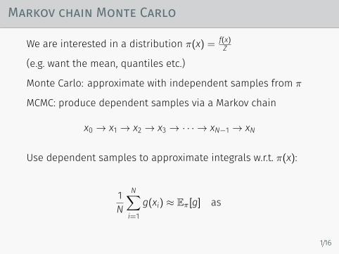
Markov chain Monte Carlo

We are interested in a distribution π(x) = f(x)Z

(e.g. want the mean, quantiles etc.)

Monte Carlo: approximate with independent samples from π

MCMC: produce dependent samples via a Markov chain

x0 → x1 → x2 → x3 → · · · → xN−1 → xN

Use dependent samples to approximate integrals w.r.t. π(x):

1N

N∑i=1

g(xi) ≈ Eπ[g] as

1/16

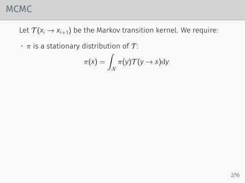
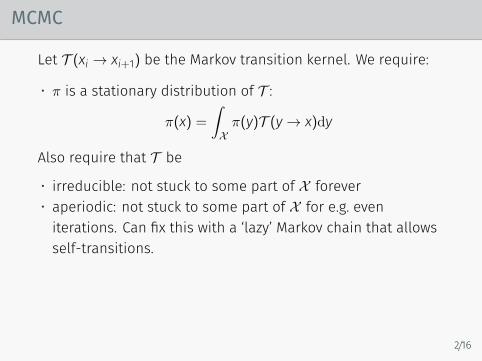
MCMC

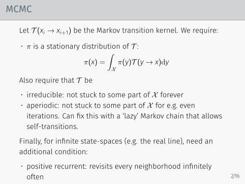
Let T (xi → xi+1) be the Markov transition kernel. We require:

• π is a stationary distribution of T :

π(x) =∫Xπ(y)T (y→ x)dy

Also require that T be

• irreducible: not stuck to some part of X forever• aperiodic: not stuck to some part of X for e.g. eveniterations. Can fix this with a ‘lazy’ Markov chain that allowsself-transitions.

Finally, for infinite state-spaces (e.g. the real line), need anadditional condition:

• positive recurrent: revisits every neighborhood infinitelyoften

2/16

MCMC

Let T (xi → xi+1) be the Markov transition kernel. We require:

• π is a stationary distribution of T :

π(x) =∫Xπ(y)T (y→ x)dy

Also require that T be

• irreducible: not stuck to some part of X forever• aperiodic: not stuck to some part of X for e.g. eveniterations. Can fix this with a ‘lazy’ Markov chain that allowsself-transitions.

Finally, for infinite state-spaces (e.g. the real line), need anadditional condition:

• positive recurrent: revisits every neighborhood infinitelyoften

2/16

MCMC

Let T (xi → xi+1) be the Markov transition kernel. We require:

• π is a stationary distribution of T :

π(x) =∫Xπ(y)T (y→ x)dy

Also require that T be

• irreducible: not stuck to some part of X forever

• aperiodic: not stuck to some part of X for e.g. eveniterations. Can fix this with a ‘lazy’ Markov chain that allowsself-transitions.

Finally, for infinite state-spaces (e.g. the real line), need anadditional condition:

• positive recurrent: revisits every neighborhood infinitelyoften

2/16

MCMC

Let T (xi → xi+1) be the Markov transition kernel. We require:

• π is a stationary distribution of T :

π(x) =∫Xπ(y)T (y→ x)dy

Also require that T be

• irreducible: not stuck to some part of X forever• aperiodic: not stuck to some part of X for e.g. eveniterations. Can fix this with a ‘lazy’ Markov chain that allowsself-transitions.

Finally, for infinite state-spaces (e.g. the real line), need anadditional condition:

• positive recurrent: revisits every neighborhood infinitelyoften

2/16

MCMC

Let T (xi → xi+1) be the Markov transition kernel. We require:

• π is a stationary distribution of T :

π(x) =∫Xπ(y)T (y→ x)dy

Also require that T be

• irreducible: not stuck to some part of X forever• aperiodic: not stuck to some part of X for e.g. eveniterations. Can fix this with a ‘lazy’ Markov chain that allowsself-transitions.

Finally, for infinite state-spaces (e.g. the real line), need anadditional condition:

• positive recurrent: revisits every neighborhood infinitelyoften 2/16

Ergodicity

With these conditions, our chain is ergodic

For any initialization:

1N

N∑i=1

g(xi) → Eπ[g] as N→ ∞ (Ergodicity)

We eventually forget the arbitrary initialization.

Typically, we discard the first B burn-in samples.

A good transition kernel has:

• A short burn-in period.• Fast mixing (small dependence across samples).

3/16

Ergodicity

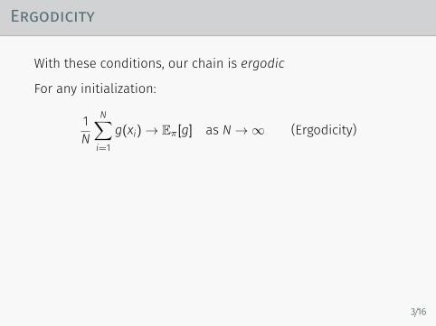
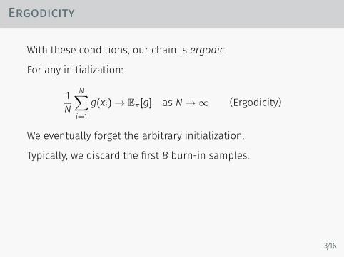
With these conditions, our chain is ergodic

For any initialization:

1N

N∑i=1

g(xi) → Eπ[g] as N→ ∞ (Ergodicity)

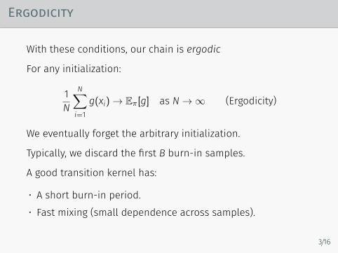
We eventually forget the arbitrary initialization.

Typically, we discard the first B burn-in samples.

A good transition kernel has:

• A short burn-in period.• Fast mixing (small dependence across samples).

3/16

Ergodicity

With these conditions, our chain is ergodic

For any initialization:

1N

N∑i=1

g(xi) → Eπ[g] as N→ ∞ (Ergodicity)

We eventually forget the arbitrary initialization.

Typically, we discard the first B burn-in samples.

A good transition kernel has:

• A short burn-in period.• Fast mixing (small dependence across samples).

3/16

Markov chain Monte Carlo

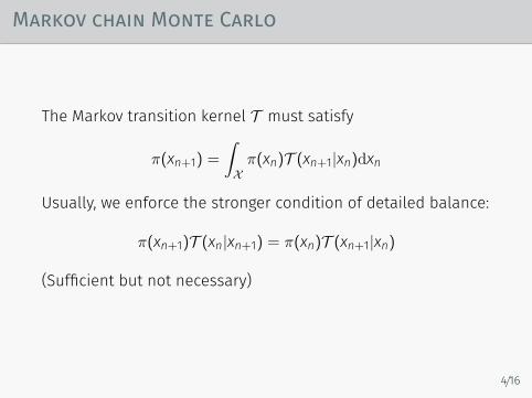
The Markov transition kernel T must satisfy

π(xn+1) =∫Xπ(xn)T (xn+1|xn)dxn

Usually, we enforce the stronger condition of detailed balance:

π(xn+1)T (xn|xn+1) = π(xn)T (xn+1|xn)

(Sufficient but not necessary)

4/16

Markov chain Monte Carlo

The Markov transition kernel T must satisfy

π(xn+1) =∫Xπ(xn)T (xn+1|xn)dxn

Usually, we enforce the stronger condition of detailed balance:

π(xn+1)T (xn|xn+1) = π(xn)T (xn+1|xn)

(Sufficient but not necessary)

4/16

The problem

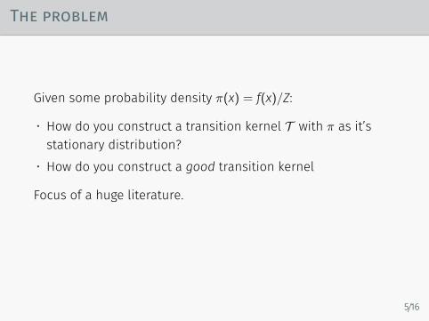
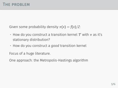
Given some probability density π(x) = f(x)/Z:

• How do you construct a transition kernel T with π as it’sstationary distribution?

• How do you construct a good transition kernel

Focus of a huge literature.

One approach: the Metropolis-Hastings algorithm

5/16

The problem

Given some probability density π(x) = f(x)/Z:

• How do you construct a transition kernel T with π as it’sstationary distribution?

• How do you construct a good transition kernel

Focus of a huge literature.

One approach: the Metropolis-Hastings algorithm

5/16

The Metropolis-Hastings algorithm

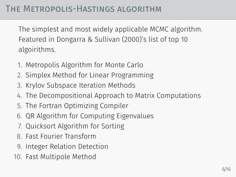
The simplest and most widely applicable MCMC algorithm.Featured in Dongarra & Sullivan (2000)’s list of top 10algoirithms.

1. Metropolis Algorithm for Monte Carlo2. Simplex Method for Linear Programming3. Krylov Subspace Iteration Methods4. The Decompositional Approach to Matrix Computations5. The Fortran Optimizing Compiler6. QR Algorithm for Computing Eigenvalues7. Quicksort Algorithm for Sorting8. Fast Fourier Transform9. Integer Relation Detection10. Fast Multipole Method

6/16

The Metropolis-Hastings algorithm

A random walk algorithm

Choose a proposal distrib. q(xnew|xold). E.g. xnew ∼ N (xold, σ2I)

Initialize chain at some starting point x0.

Repeat:

• Propose a new point x∗ according to q(x∗|xn).• Define α = min

(1, π(x

∗)q(xn|x∗)π(xn)q(x∗|xn)

)= min

(1, f(x

∗)q(xn|x∗)f(xn)q(x∗|xn)

)• Set xn+1 = x∗ with probability α, else xn+1 = xn.

Comments:

• Do not need to calculate the normalization constant Z.• Accept/reject steps ensure this has the correct distribution.• On rejection, keep old sample (i.e. there will be repetition)

7/16

The Metropolis-Hastings algorithm

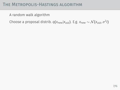
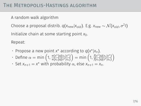
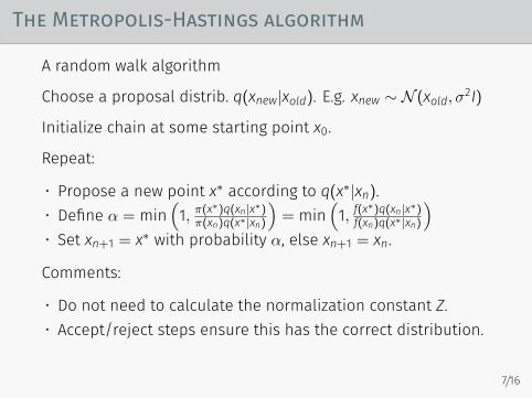
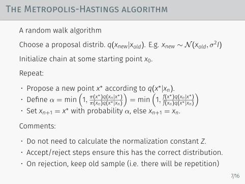
A random walk algorithm

Choose a proposal distrib. q(xnew|xold). E.g. xnew ∼ N (xold, σ2I)

Initialize chain at some starting point x0.

Repeat:

• Propose a new point x∗ according to q(x∗|xn).• Define α = min

(1, π(x

∗)q(xn|x∗)π(xn)q(x∗|xn)

)= min

(1, f(x

∗)q(xn|x∗)f(xn)q(x∗|xn)

)• Set xn+1 = x∗ with probability α, else xn+1 = xn.

Comments:

• Do not need to calculate the normalization constant Z.• Accept/reject steps ensure this has the correct distribution.• On rejection, keep old sample (i.e. there will be repetition)

7/16

The Metropolis-Hastings algorithm

A random walk algorithm

Choose a proposal distrib. q(xnew|xold). E.g. xnew ∼ N (xold, σ2I)

Initialize chain at some starting point x0.

Repeat:

• Propose a new point x∗ according to q(x∗|xn).• Define α = min

(1, π(x

∗)q(xn|x∗)π(xn)q(x∗|xn)

)= min

(1, f(x

∗)q(xn|x∗)f(xn)q(x∗|xn)

)• Set xn+1 = x∗ with probability α, else xn+1 = xn.

Comments:

• Do not need to calculate the normalization constant Z.• Accept/reject steps ensure this has the correct distribution.

• On rejection, keep old sample (i.e. there will be repetition)

7/16

The Metropolis-Hastings algorithm

A random walk algorithm

Choose a proposal distrib. q(xnew|xold). E.g. xnew ∼ N (xold, σ2I)

Initialize chain at some starting point x0.

Repeat:

• Propose a new point x∗ according to q(x∗|xn).• Define α = min

(1, π(x

∗)q(xn|x∗)π(xn)q(x∗|xn)

)= min

(1, f(x

∗)q(xn|x∗)f(xn)q(x∗|xn)

)• Set xn+1 = x∗ with probability α, else xn+1 = xn.

Comments:

• Do not need to calculate the normalization constant Z.• Accept/reject steps ensure this has the correct distribution.• On rejection, keep old sample (i.e. there will be repetition)

7/16

The Metropolis-Hastings algorithm

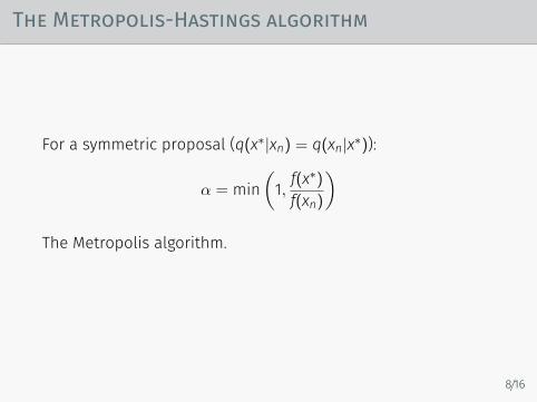
For a symmetric proposal (q(x∗|xn) = q(xn|x∗)):

α = min(1, f(x

∗)

f(xn)

)

The Metropolis algorithm.

8/16

The Metropolis-Hastings algorithm

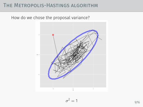
How do we chose the proposal variance?

−2

0

2

−2 0 2x

y

σ2 = 1 9/16

The Metropolis-Hastings algorithm

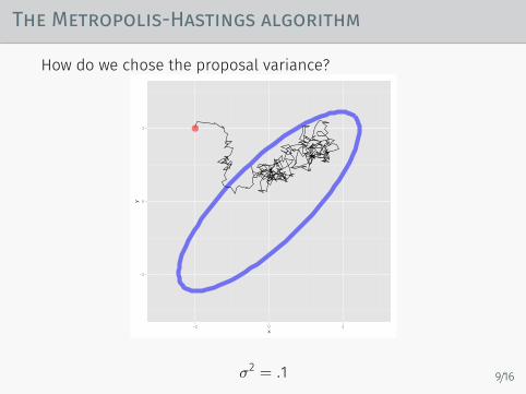
How do we chose the proposal variance?

−2

0

2

−2 0 2x

y

σ2 = .1 9/16

The Metropolis-Hastings algorithm

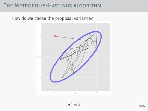
How do we chose the proposal variance?

−2

0

2

−2 0 2x

y

σ2 = 5 9/16

Does this satisfy detailed balance?

First, what is the transition kernel T (xn+1|xn)?

Prob. of moving from xn to xn+1 is α(xn+1, xn)q(xn+1|xn).

Prob. of accepting move at xn is α(x) =∫X α(y, xn)q(y|xn)dy.

Prob. of rejection at xn is r(xn) = 1− α(xn).

We then have:

T (xn+1|xn) = α(xn+1, xn)q(xn+1|xn) + r(xn)δ(xn = xn+1)

We want to show detailed balance:

π(xn)T (xn+1|xn) = π(xn+1)T (xn|xn+1)

10/16

Does this satisfy detailed balance?

First, what is the transition kernel T (xn+1|xn)?

Prob. of moving from xn to xn+1 is α(xn+1, xn)q(xn+1|xn).

Prob. of accepting move at xn is α(x) =∫X α(y, xn)q(y|xn)dy.

Prob. of rejection at xn is r(xn) = 1− α(xn).

We then have:

T (xn+1|xn) = α(xn+1, xn)q(xn+1|xn) + r(xn)δ(xn = xn+1)

We want to show detailed balance:

π(xn)T (xn+1|xn) = π(xn+1)T (xn|xn+1)

10/16

Does this satisfy detailed balance?

First, what is the transition kernel T (xn+1|xn)?

Prob. of moving from xn to xn+1 is α(xn+1, xn)q(xn+1|xn).

Prob. of accepting move at xn is α(x) =∫X α(y, xn)q(y|xn)dy.

Prob. of rejection at xn is r(xn) = 1− α(xn).

We then have:

T (xn+1|xn) = α(xn+1, xn)q(xn+1|xn) + r(xn)δ(xn = xn+1)

We want to show detailed balance:

π(xn)T (xn+1|xn) = π(xn+1)T (xn|xn+1)

10/16

Does this satisfy detailed balance?

First, what is the transition kernel T (xn+1|xn)?

Prob. of moving from xn to xn+1 is α(xn+1, xn)q(xn+1|xn).

Prob. of accepting move at xn is α(x) =∫X α(y, xn)q(y|xn)dy.

Prob. of rejection at xn is r(xn) = 1− α(xn).

We then have:

T (xn+1|xn) = α(xn+1, xn)q(xn+1|xn) + r(xn)δ(xn = xn+1)

We want to show detailed balance:

π(xn)T (xn+1|xn) = π(xn+1)T (xn|xn+1)

10/16

Does this satisfy detailed balance?

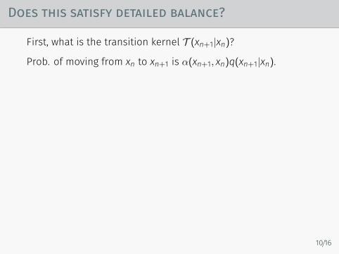
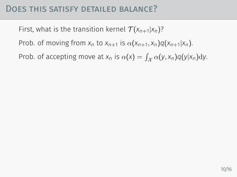
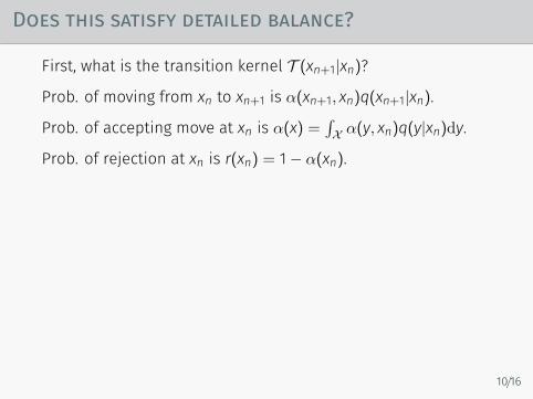
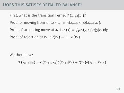
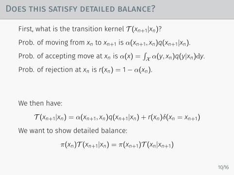
First, what is the transition kernel T (xn+1|xn)?

Prob. of moving from xn to xn+1 is α(xn+1, xn)q(xn+1|xn).

Prob. of accepting move at xn is α(x) =∫X α(y, xn)q(y|xn)dy.

Prob. of rejection at xn is r(xn) = 1− α(xn).

We then have:

T (xn+1|xn) = α(xn+1, xn)q(xn+1|xn) + r(xn)δ(xn = xn+1)

We want to show detailed balance:

π(xn)T (xn+1|xn) = π(xn+1)T (xn|xn+1)

10/16

Does this satisfy detailed balance?

First, what is the transition kernel T (xn+1|xn)?

Prob. of moving from xn to xn+1 is α(xn+1, xn)q(xn+1|xn).

Prob. of accepting move at xn is α(x) =∫X α(y, xn)q(y|xn)dy.

Prob. of rejection at xn is r(xn) = 1− α(xn).

We then have:

T (xn+1|xn) = α(xn+1, xn)q(xn+1|xn) + r(xn)δ(xn = xn+1)

We want to show detailed balance:

π(xn)T (xn+1|xn) = π(xn+1)T (xn|xn+1)

10/16

The Metropolis-Hastings algorithm

Detailed balance: π(xn)T (xn+1|xn) = π(xn+1)T (xn|xn+1)

Consider the LHS:

π(xn)T (xn+1|xn) = π(xn) (α(xn+1, xn)q(xn+1, xn) + r(xn)δ(xn = xn+1))

The first term is:f(xn)Z min

(1, f(xn+1)q(xn|xn+1)f(xn)q(xn+1|xn)

)q(xn+1|xn)

=1Z min (f(xn)q(xn+1|xn), f(xn+1)q(xn|xn+1))

The second term takes this form too. Thus

π(xn)T (xn+1|xn) = π(xn+1)T (xn|xn+1)

11/16

The Metropolis-Hastings algorithm

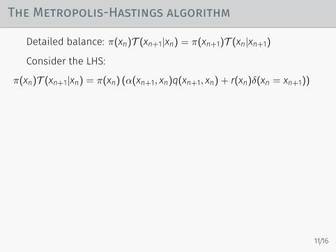
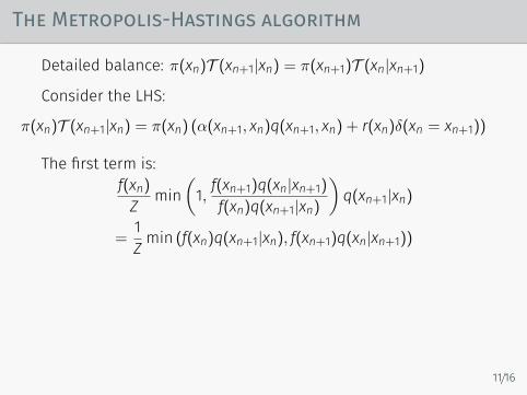
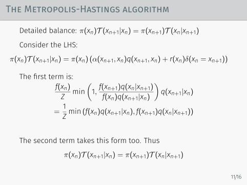
Detailed balance: π(xn)T (xn+1|xn) = π(xn+1)T (xn|xn+1)

Consider the LHS:

π(xn)T (xn+1|xn) = π(xn) (α(xn+1, xn)q(xn+1, xn) + r(xn)δ(xn = xn+1))

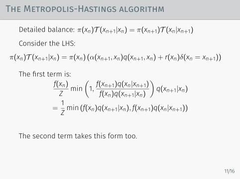
The first term is:f(xn)Z min

(1, f(xn+1)q(xn|xn+1)f(xn)q(xn+1|xn)

)q(xn+1|xn)

=1Z min (f(xn)q(xn+1|xn), f(xn+1)q(xn|xn+1))

The second term takes this form too. Thus

π(xn)T (xn+1|xn) = π(xn+1)T (xn|xn+1)

11/16

The Metropolis-Hastings algorithm

Detailed balance: π(xn)T (xn+1|xn) = π(xn+1)T (xn|xn+1)

Consider the LHS:

π(xn)T (xn+1|xn) = π(xn) (α(xn+1, xn)q(xn+1, xn) + r(xn)δ(xn = xn+1))

The first term is:f(xn)Z min

(1, f(xn+1)q(xn|xn+1)f(xn)q(xn+1|xn)

)q(xn+1|xn)

=1Z min (f(xn)q(xn+1|xn), f(xn+1)q(xn|xn+1))

The second term takes this form too.

Thus

π(xn)T (xn+1|xn) = π(xn+1)T (xn|xn+1)

11/16

The Metropolis-Hastings algorithm

Detailed balance: π(xn)T (xn+1|xn) = π(xn+1)T (xn|xn+1)

Consider the LHS:

π(xn)T (xn+1|xn) = π(xn) (α(xn+1, xn)q(xn+1, xn) + r(xn)δ(xn = xn+1))

The first term is:f(xn)Z min

(1, f(xn+1)q(xn|xn+1)f(xn)q(xn+1|xn)

)q(xn+1|xn)

=1Z min (f(xn)q(xn+1|xn), f(xn+1)q(xn|xn+1))

The second term takes this form too. Thus

π(xn)T (xn+1|xn) = π(xn+1)T (xn|xn+1)

11/16

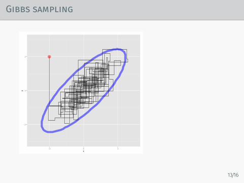
Gibbs sampling

Consider a Markov chain on over a set of variables (x1, · · · , xd).

Gibbs sampling cycles though these sequentially (orrandomly).At the ith step, it updates xi conditioned on the the rest:

xi ∼ π(xi|x1, . . . , xi−1, xi+1, . . . , xn) = π(xi|x\i)

Often these conditionals have a much simpler form than thejoint.

12/16

Gibbs sampling

−2

0

2

−2 0 2x

y

13/16

Detailed balance for the sequential Gibbs sampler

Does it satisfy stationarity?

Does it satisfy irreducibility?

Is it aperiodic?

14/16

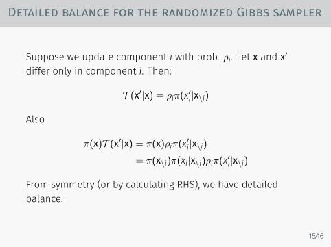
Detailed balance for the randomized Gibbs sampler

Suppose we update component i with prob. ρi. Let x and x′

differ only in component i. Then:

T (x′|x) = ρiπ(x′i|x\i)

Also

π(x)T (x′|x) = π(x)ρiπ(x′i|x\i)= π(x\i)π(xi|x\i)ρiπ(x′i|x\i)

From symmetry (or by calculating RHS), we have detailedbalance.

15/16

Detailed balance for Gibbs sampler

Under mild conditions, Gibbs sampling is irreducible.

Can break down under constraints. E.g. two perfectly couplevariables.Performance deteriorates with strong coupling betweenvariables.Poor mixing due to coupled variables is always a concern.

Advantages: Simple, with no free parameters.Often, conditional independencies in a model along withsuitable conjugate priors allow efficient ‘blocked-Gibbssamplers’.

16/16

Detailed balance for Gibbs sampler

Under mild conditions, Gibbs sampling is irreducible.Can break down under constraints. E.g. two perfectly couplevariables.Performance deteriorates with strong coupling betweenvariables.Poor mixing due to coupled variables is always a concern.

Advantages: Simple, with no free parameters.Often, conditional independencies in a model along withsuitable conjugate priors allow efficient ‘blocked-Gibbssamplers’.

16/16

Detailed balance for Gibbs sampler

Under mild conditions, Gibbs sampling is irreducible.Can break down under constraints. E.g. two perfectly couplevariables.Performance deteriorates with strong coupling betweenvariables.Poor mixing due to coupled variables is always a concern.

Advantages: Simple, with no free parameters.

Often, conditional independencies in a model along withsuitable conjugate priors allow efficient ‘blocked-Gibbssamplers’.

16/16

Detailed balance for Gibbs sampler

Under mild conditions, Gibbs sampling is irreducible.Can break down under constraints. E.g. two perfectly couplevariables.Performance deteriorates with strong coupling betweenvariables.Poor mixing due to coupled variables is always a concern.

Advantages: Simple, with no free parameters.Often, conditional independencies in a model along withsuitable conjugate priors allow efficient ‘blocked-Gibbssamplers’.

16/16