Hidden Markov Models - University of Texas
33
Hidden Markov Models Adapted from Dr Catherine Sweeney-Reed’s slides
Transcript of Hidden Markov Models - University of Texas

Hidden MarkovModels
Adapted fromDr Catherine Sweeney-Reed’sslides
Summary
Introduction Description Central problems in HMM modelling Extensions Demonstration
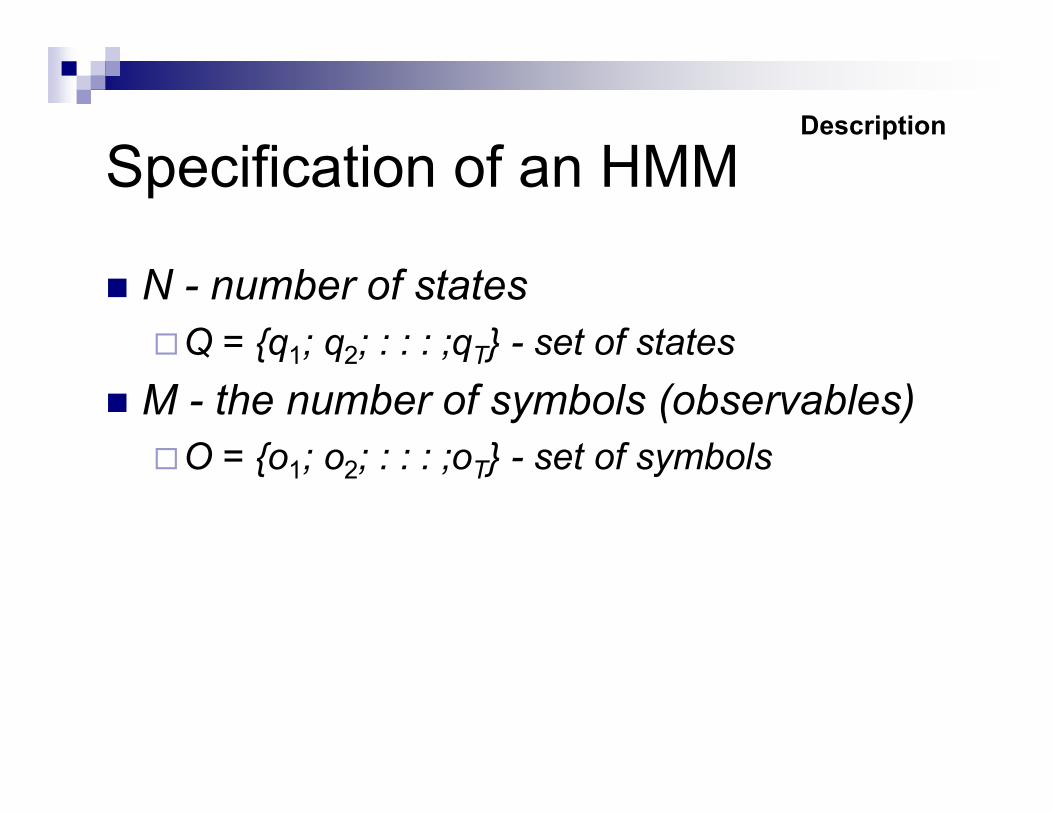
Specification of an HMM
N - number of statesQ = {q1; q2; : : : ;qT} - set of states
M - the number of symbols (observables)O = {o1; o2; : : : ;oT} - set of symbols
Description
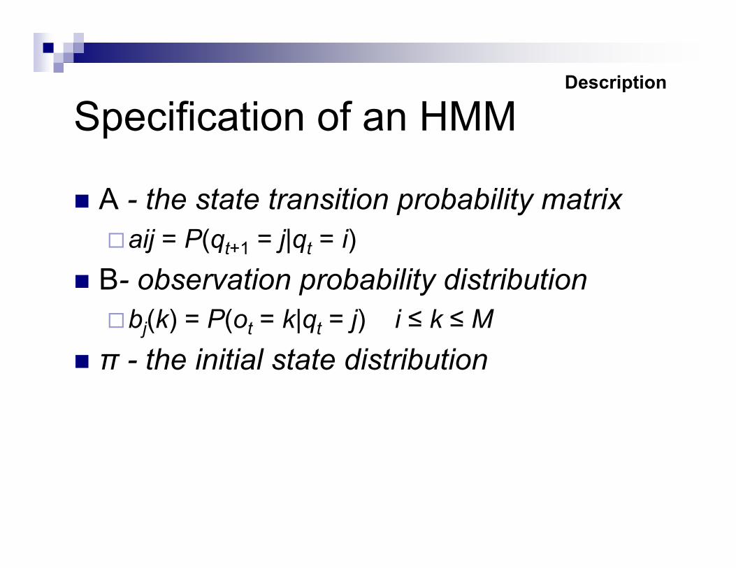
Specification of an HMM
A - the state transition probability matrixaij = P(qt+1 = j|qt = i)
B- observation probability distributionbj(k) = P(ot = k|qt = j) i ≤ k ≤ M
π - the initial state distribution
Description
Specification of an HMM
Full HMM is thus specified as a triplet:λ = (A,B,π)
Description
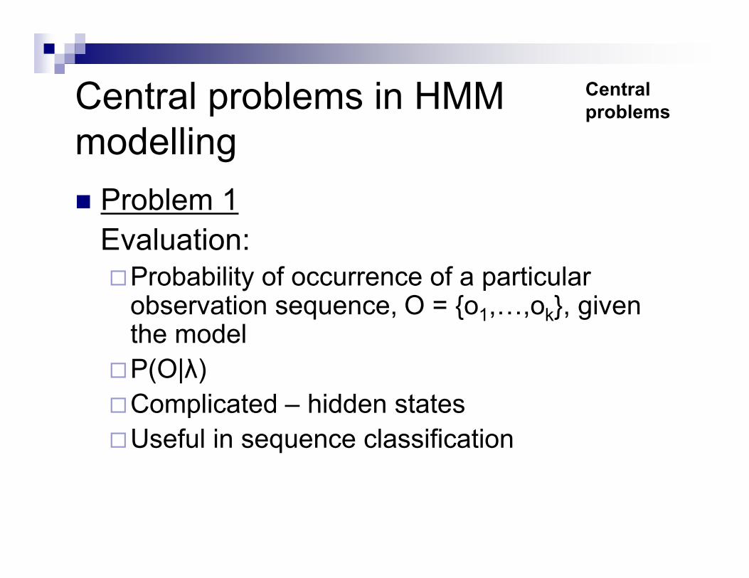
Central problems in HMMmodelling Problem 1
Evaluation:Probability of occurrence of a particular
observation sequence, O = {o1,…,ok}, giventhe model
P(O|λ)Complicated – hidden statesUseful in sequence classification
Centralproblems
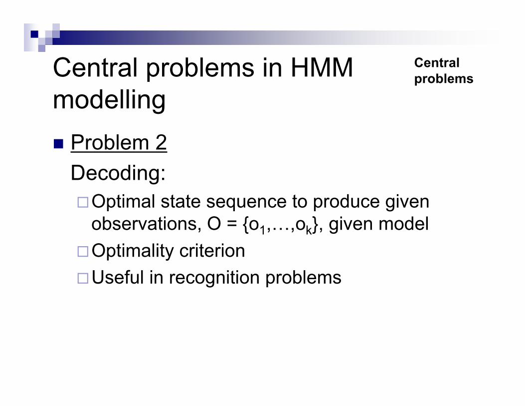
Central problems in HMMmodelling Problem 2
Decoding:Optimal state sequence to produce given
observations, O = {o1,…,ok}, given modelOptimality criterionUseful in recognition problems
Centralproblems
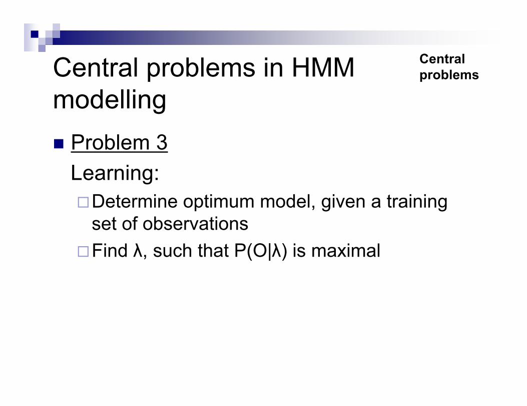
Central problems in HMMmodelling Problem 3
Learning:Determine optimum model, given a training
set of observationsFind λ, such that P(O|λ) is maximal
Centralproblems
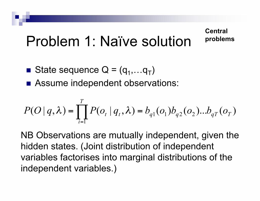
Problem 1: Naïve solution
State sequence Q = (q1,…qT) Assume independent observations:
)()...()(),|(,|( 2211
1
TqTqqt
T
i
t obobobqoPqOP ==) !=
""
Centralproblems
NB Observations are mutually independent, given thehidden states. (Joint distribution of independentvariables factorises into marginal distributions of theindependent variables.)
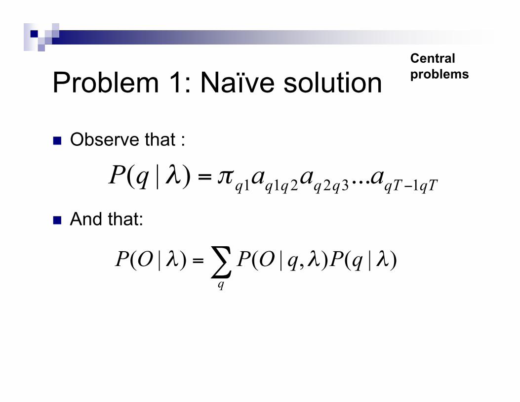
Problem 1: Naïve solution
Observe that :
And that:
qTqTqqqqq aaaqP 132211 ...)|( != "#
Centralproblems
!=q
qPqOPOP )|(),|()|( """
Problem 1: Naïve solution
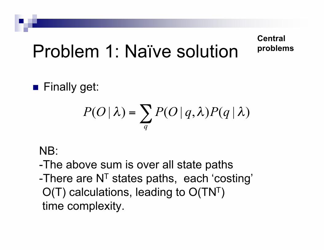
Finally get:
Centralproblems
!=q
qPqOPOP )|(),|()|( """
NB:-The above sum is over all state paths-There are NT states paths, each ‘costing’ O(T) calculations, leading to O(TNT) time complexity.
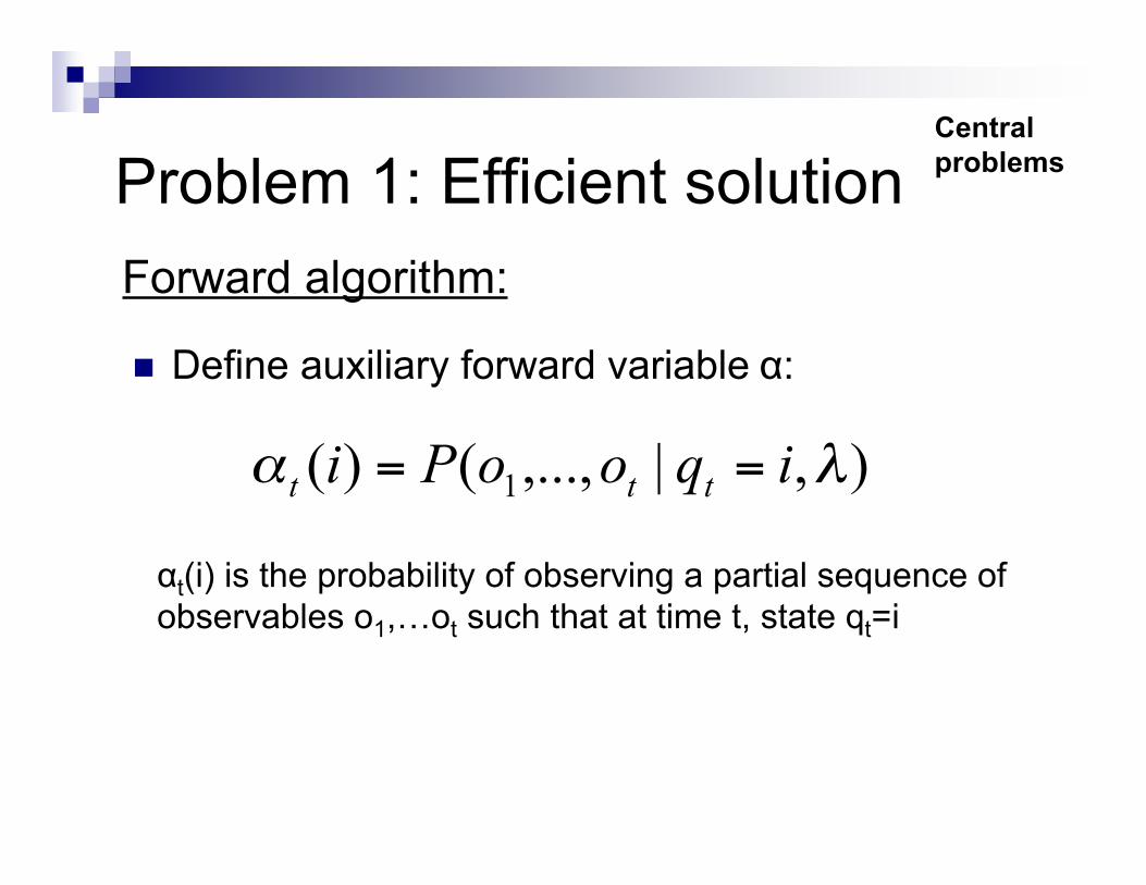
Problem 1: Efficient solution
Define auxiliary forward variable α:
Centralproblems
),|,...,()( 1 !" iqooPi ttt ==
αt(i) is the probability of observing a partial sequence ofobservables o1,…ot such that at time t, state qt=i
Forward algorithm:
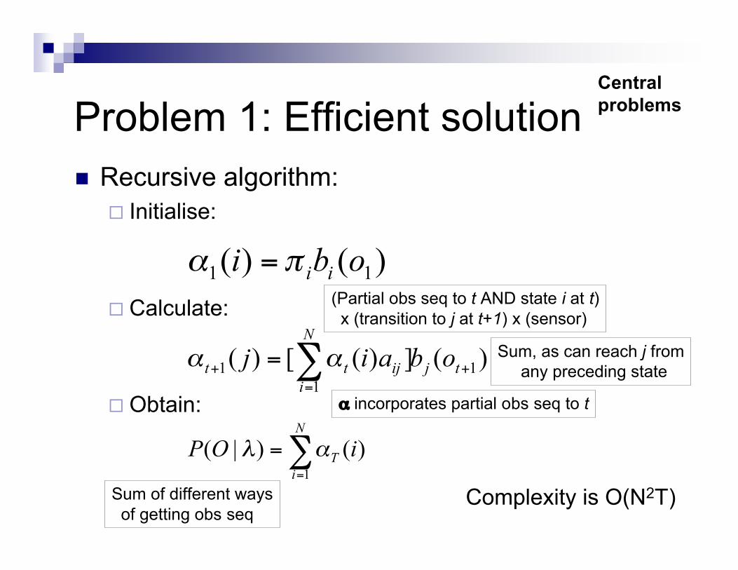
Problem 1: Efficient solution Recursive algorithm:
Initialise:
Calculate:
Obtain:
)()( 11 obiii
!" =
Centralproblems
)(])([)( 1
1
1 +
=
+ != tj
N
i
ijtt obaij ""
!=
=N
i
TiOP
1
)()|( "#
Complexity is O(N2T)
(Partial obs seq to t AND state i at t) x (transition to j at t+1) x (sensor)
Sum of different ways of getting obs seq
Sum, as can reach j from any preceding state
α incorporates partial obs seq to t
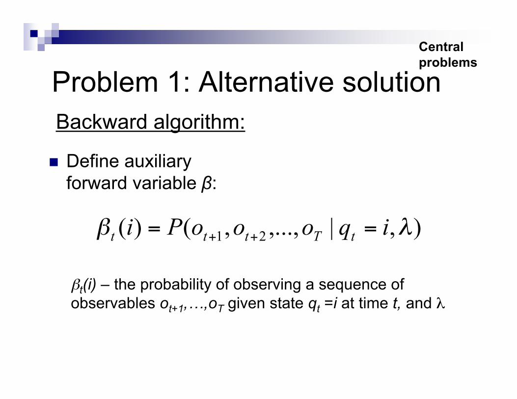
Problem 1: Alternative solution
Define auxiliaryforward variable β:
Centralproblems
Backward algorithm:
),|,...,,()( 21 !" iqoooPi tTttt == ++
βt(i) – the probability of observing a sequence ofobservables ot+1,…,oT given state qt =i at time t, and λ
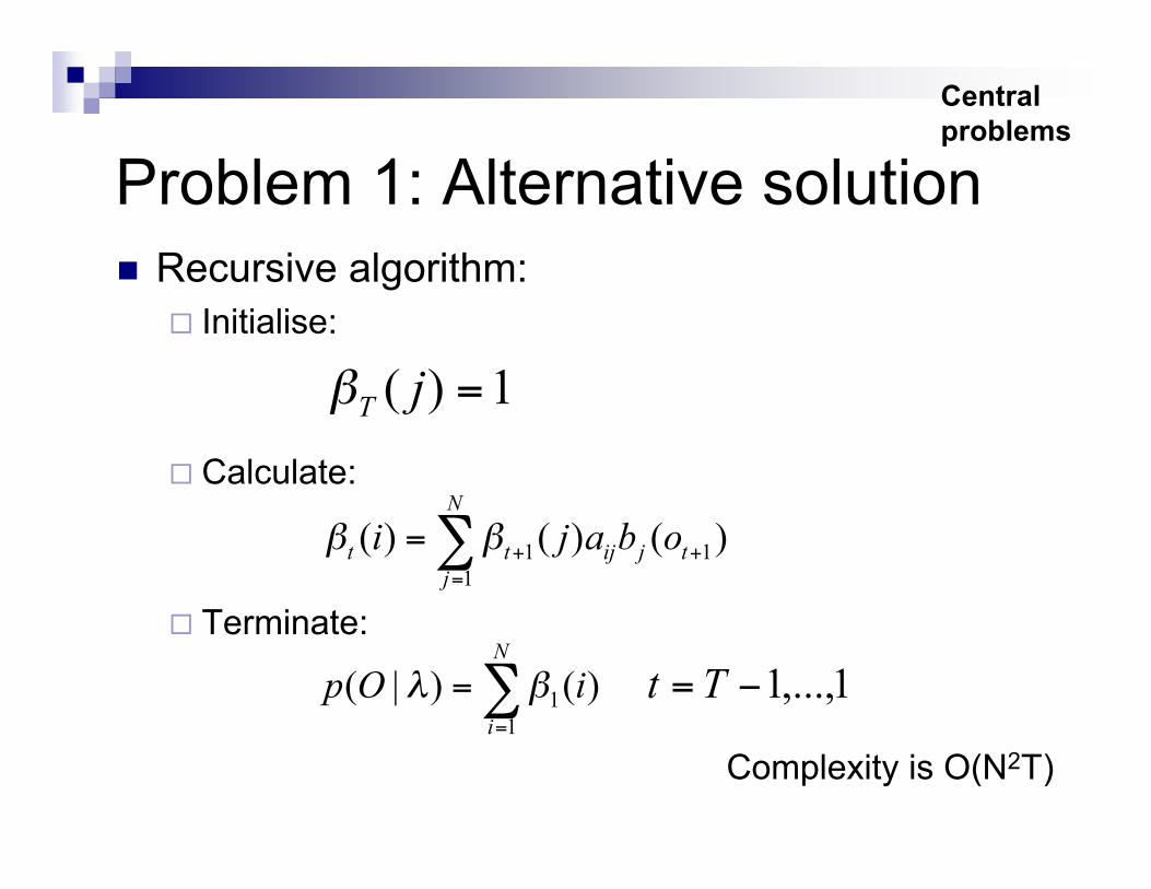
Problem 1: Alternative solution Recursive algorithm:
Initialise:
Calculate:
Terminate:
1)( =jT!
Centralproblems
Complexity is O(N2T)
1 1
1
( ) ( ) ( )N
t t ij j t
j
i j a b o! !+ +
=
="
!=
=N
i
iOp1
1 )()|( "# 1,...,1!= Tt
Problem 2: Decoding
Choose state sequence to maximiseprobability of observation sequence
Viterbi algorithm - inductive algorithm thatkeeps the best state sequence at eachinstance
Centralproblems
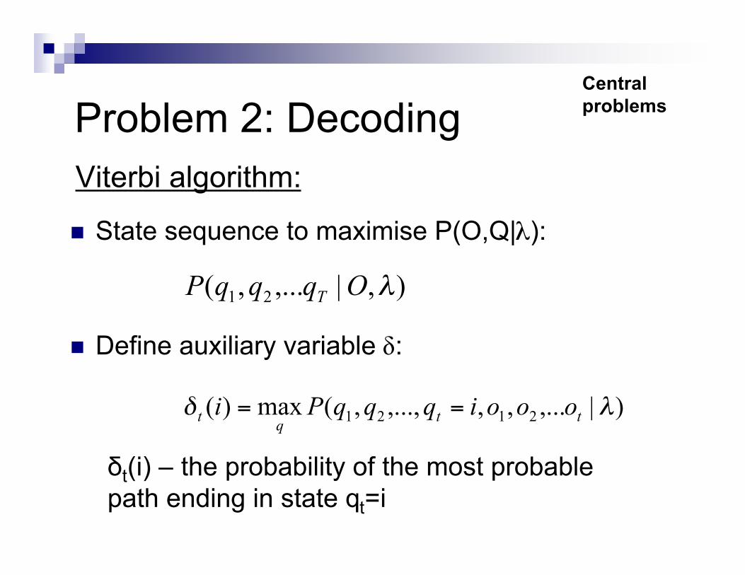
Problem 2: Decoding
State sequence to maximise P(O,Q|λ):
Define auxiliary variable δ:
),|,...,( 21 !OqqqP T
Viterbi algorithm:
Centralproblems
)|,...,,,...,,(max)( 2121 !" ttq
t oooiqqqPi ==
δt(i) – the probability of the most probablepath ending in state qt=i
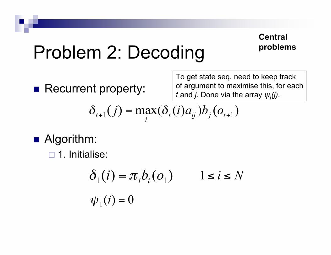
Problem 2: Decoding
Recurrent property:
Algorithm: 1. Initialise:
)())((max)( 11 ++ = tjijti
t obaij !!
Centralproblems
)()( 11 obiii
!" = Ni !!1
0)(1 =i!
To get state seq, need to keep trackof argument to maximise this, for eacht and j. Done via the array ψt(j).
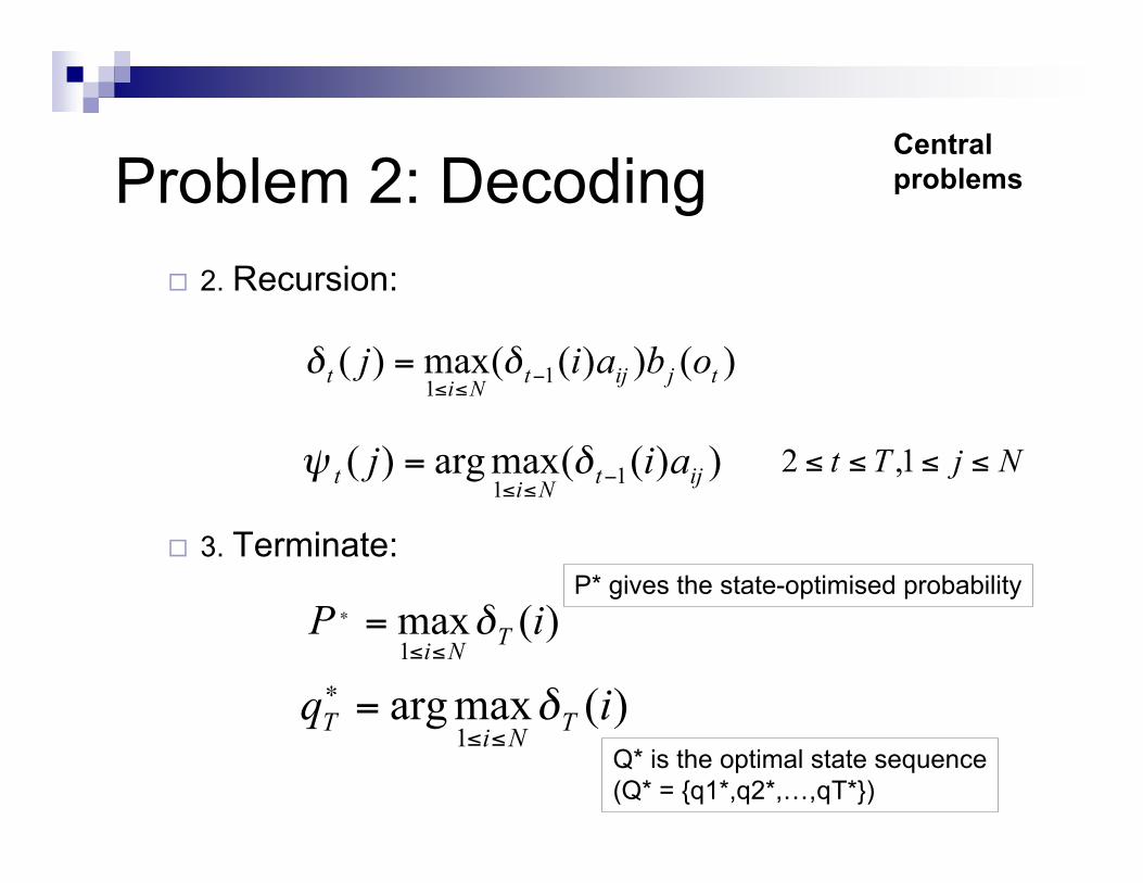
Problem 2: Decoding 2. Recursion:
3. Terminate:
)())((max)( 11
tjijtNi
t obaij !""
= ##
Centralproblems
))((maxarg)( 11
ijtNi
t aij !""
= #$ NjTt !!!! 1,2
)(max1
iPT
Ni
!""
=#
)(maxarg1
iq TNi
T !""
#=
P* gives the state-optimised probability
Q* is the optimal state sequence(Q* = {q1*,q2*,…,qT*})
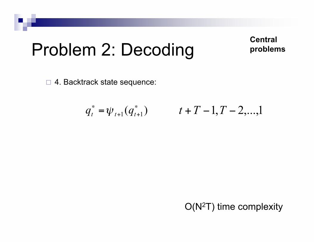
Problem 2: Decoding
4. Backtrack state sequence:
)( 11
!
++
!=
tttqq " 1,...,2,1 !!+ TTt
O(N2T) time complexity
Centralproblems
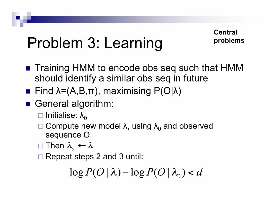
Problem 3: Learning Training HMM to encode obs seq such that HMM
should identify a similar obs seq in future Find λ=(A,B,π), maximising P(O|λ) General algorithm:
Initialise: λ0 Compute new model λ, using λ0 and observed
sequence O Then Repeat steps 2 and 3 until:
!! "o
Centralproblems
dOPOP <! )|(log)|(log 0""
Problem 3: Learning
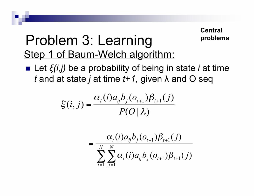
Let ξ(i,j) be a probability of being in state i at timet and at state j at time t+1, given λ and O seq
)|(
)()()(),(
11
!
"#$
OP
jobaiji
ttjijt ++=
Centralproblems
!!= =
++
++=
N
i
N
j
ttjijt
ttjijt
jobai
jobai
1 1
11
11
)()()(
)()()(
"#
"#
Step 1 of Baum-Welch algorithm:
Problem 3: LearningCentralproblems
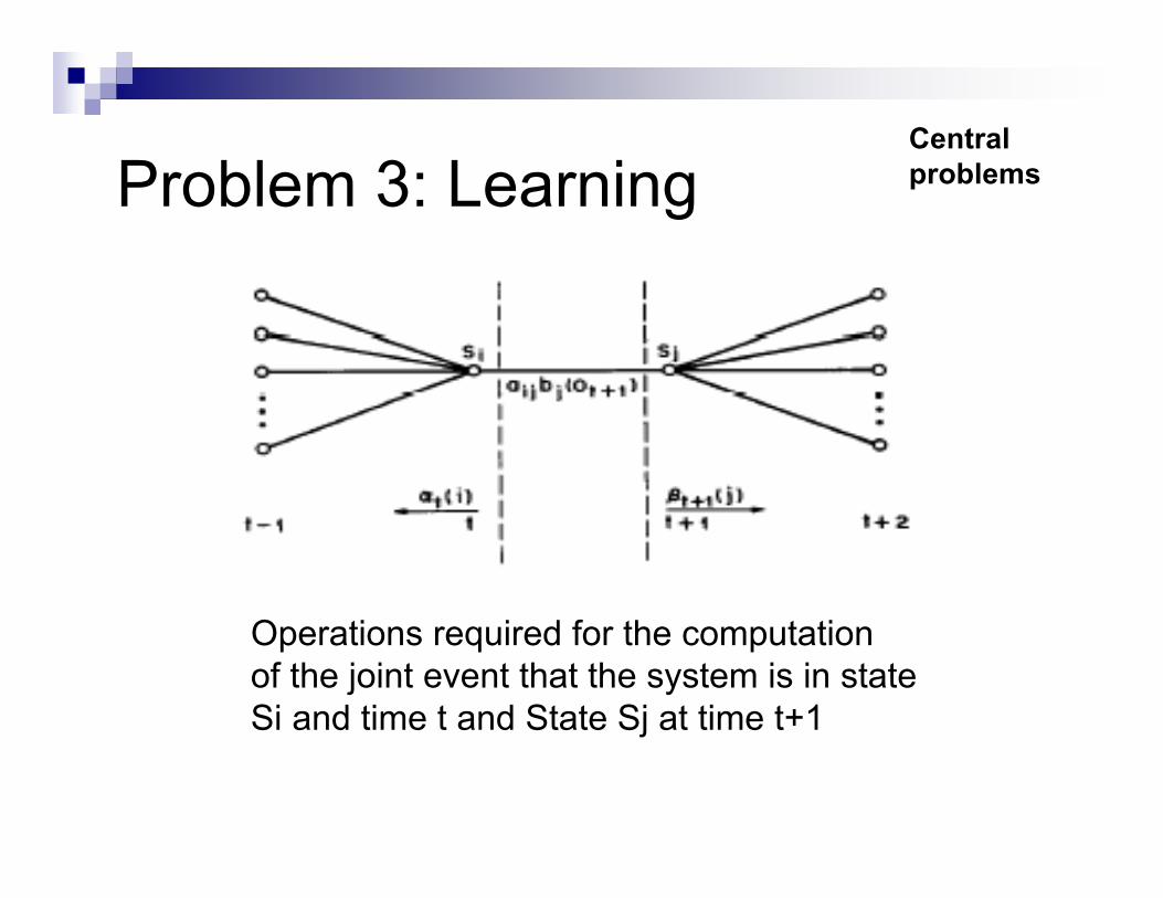
Operations required for the computationof the joint event that the system is in stateSi and time t and State Sj at time t+1
Problem 3: Learning
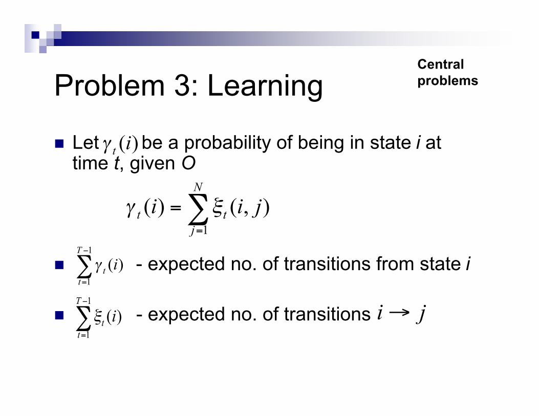
Let be a probability of being in state i attime t, given O
- expected no. of transitions from state i
- expected no. of transitions
!=
=N
j
tt jii1
),()( "#
Centralproblems
1
1
( )T
t
t
i!"
=
#
1
1
( )T
t
t
i!"
=
# ji!
( )ti!
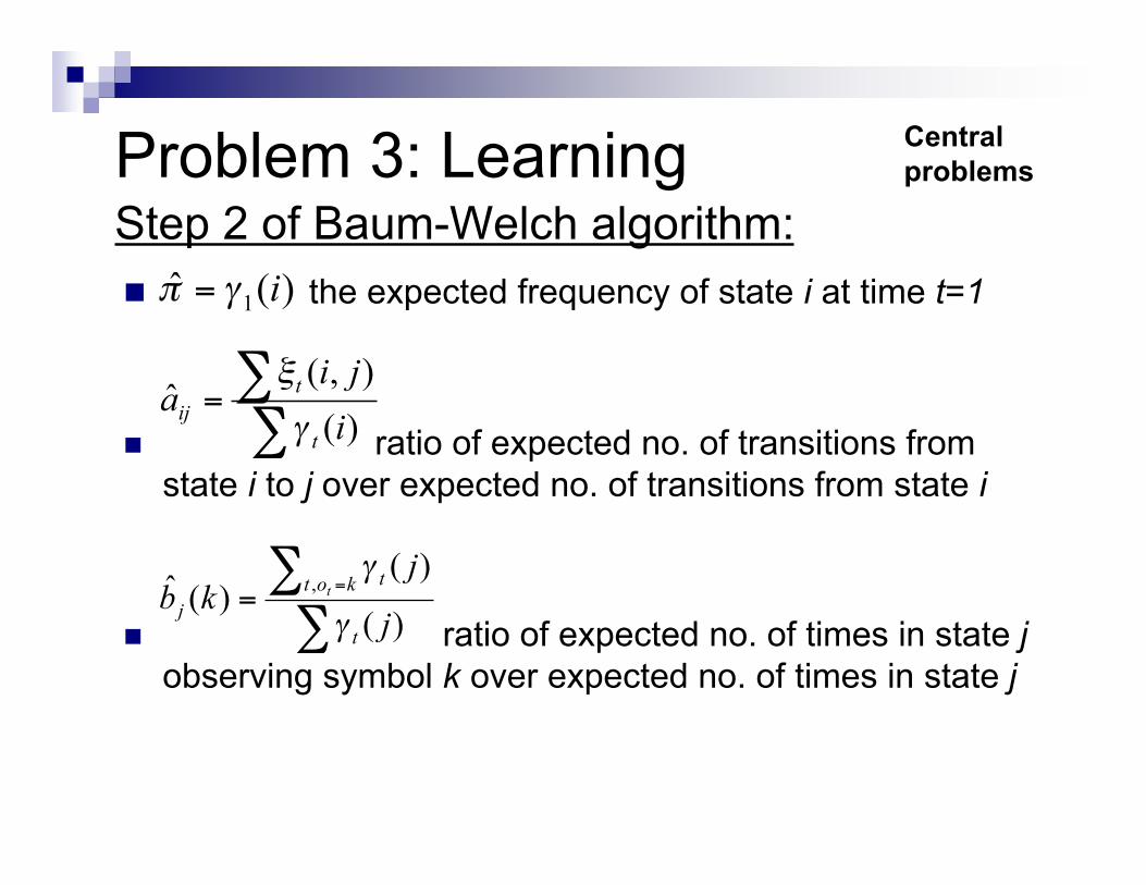
Problem 3: Learning
the expected frequency of state i at time t=1
ratio of expected no. of transitions fromstate i to j over expected no. of transitions from state i
ratio of expected no. of times in state jobserving symbol k over expected no. of times in state j
!!
=)(
),(ˆ
i
jia
t
t
ij"
#
Centralproblems
Step 2 of Baum-Welch algorithm:
!! =
=)(
)()(ˆ
,
j
jkb
t
kot t
jt
"
"
)(ˆ1 i!" =
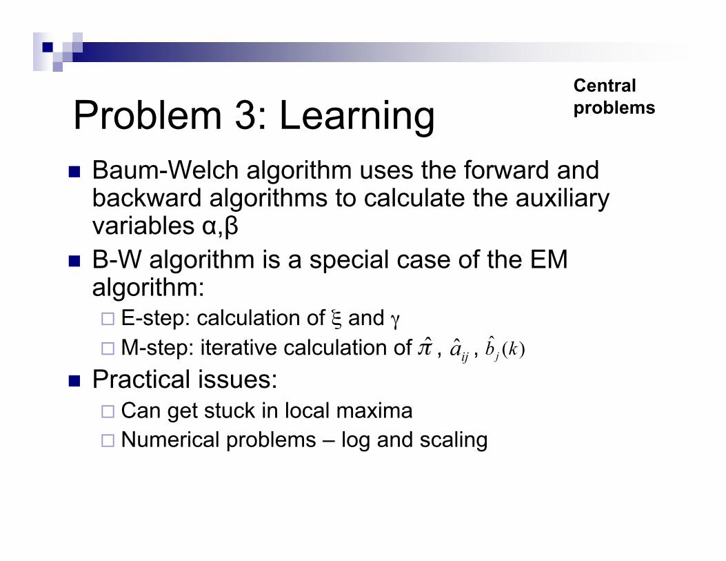
Problem 3: Learning Baum-Welch algorithm uses the forward and
backward algorithms to calculate the auxiliaryvariables α,β
B-W algorithm is a special case of the EMalgorithm: E-step: calculation of ξ and γ M-step: iterative calculation of , ,
Practical issues: Can get stuck in local maxima Numerical problems – log and scaling
!ija )(ˆ kbj
Centralproblems
Extensions
Problem-specific:Left to right HMM (speech recognition)Profile HMM (bioinformatics)
Extensions
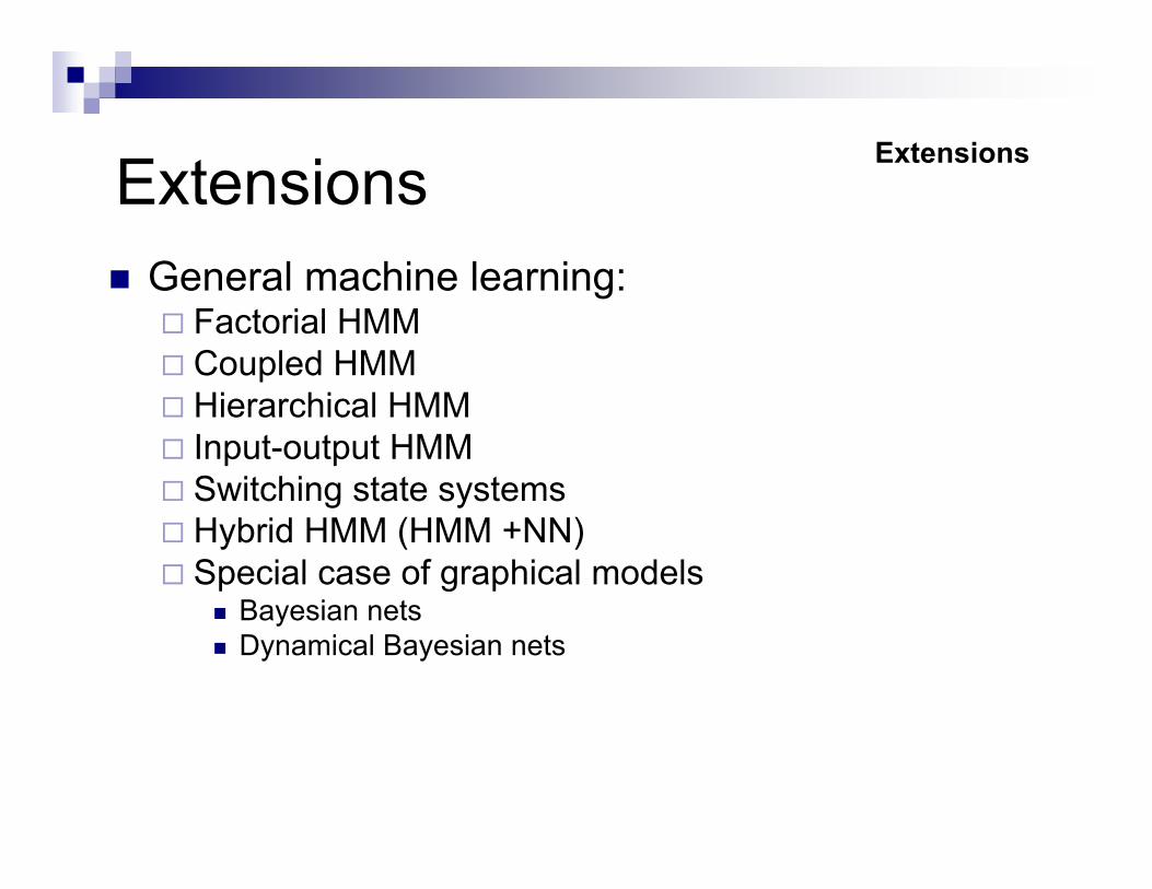
Extensions General machine learning:
Factorial HMM Coupled HMM Hierarchical HMM Input-output HMM Switching state systems Hybrid HMM (HMM +NN) Special case of graphical models
Bayesian nets Dynamical Bayesian nets
Extensions
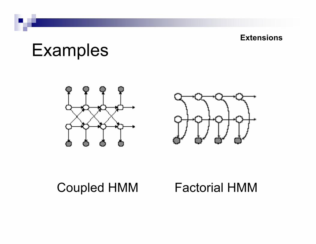
ExamplesExtensions
Coupled HMM Factorial HMM
HMMs – Sleep Staging
Flexer, Sykacek, Rezek, and Dorffner (2000) Observation sequence: EEG data Fit model to data according to 3 sleep stages
to produce continuous probabilities: P(wake),P(deep), and P(REM)
Hidden states correspond with recognisedsleep stages. 3 continuous probability plots,giving P of each at every second
Demonstrations
HMMs – Sleep Staging
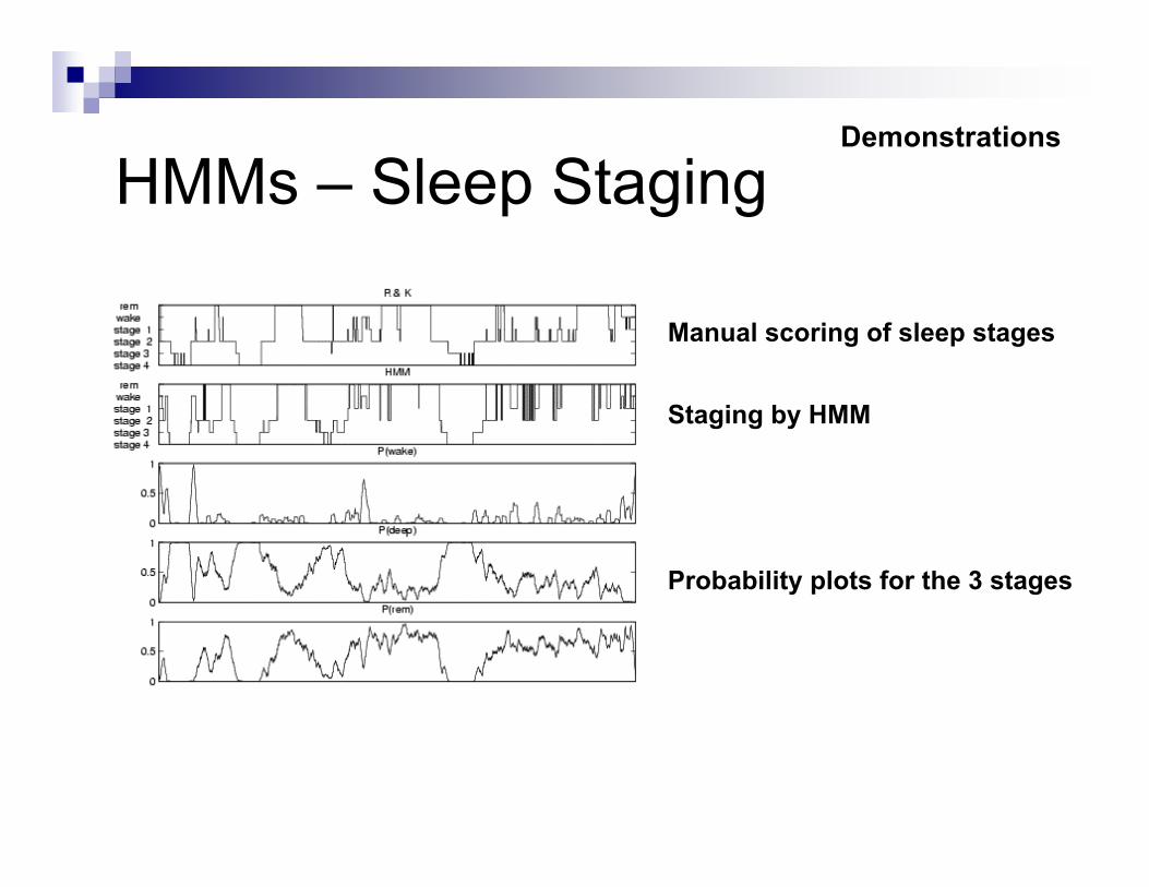
Probability plots for the 3 stages
Staging by HMM
Manual scoring of sleep stages
Demonstrations

Excel
Demonstration of a working HMMimplemented in Excel
Demonstrations
Further Reading
L. R. Rabiner, "A tutorial on Hidden Markov Models andselected applications in speech recognition,"Proceedings of the IEEE, vol. 77, pp. 257-286, 1989.
R. Dugad and U. B. Desai, "A tutorial on Hidden Markovmodels," Signal Processing and Artifical NeuralNetworks Laboratory, Dept of Electrical Engineering,Indian Institute of Technology, Bombay Technical ReportNo.: SPANN-96.1, 1996.
W.H. Laverty, M.J. Miket, and I.W. Kelly, “Simulation ofHidden Markov Models with EXCEL”, The Statistician,vol. 51, Part 1, pp. 31-40, 2002