Hidden Markov Methods. Algorithms and Implementation

Final Project Report. MATH 127.

Nasser M. Abbasi

Course taken during Fall 2002 page compiled on July 2, 2015 at 12:08am

Contents

1 Example HMM 5

2 Forward α algorithm 72.1 Calculation of the alpha’s using logarithms . . . . . . . . . . . . . . . . . . . . . . . . . . . . . . 9

3 Backward β algorithm 11

4 Viterbi algorithm 13

5 Configuration file description 15

6 Configuration file examples 166.1 Example 1. Casino example . . . . . . . . . . . . . . . . . . . . . . . . . . . . . . . . . . . . . . . 166.2 Example 2. Homework problem 4.1 . . . . . . . . . . . . . . . . . . . . . . . . . . . . . . . . . . . 16

7 SHMM User interface 16

8 Source code description 17

9 Installation instructions 17

Abstract

Hidden Markov Models (HMM) main algorithms (forward, backward, and Viterbi) are outlined, and a GUIbased implementation (in MATLAB) of a basic HMM is included along with a user guide. The implementationuses a flexible plain text configuration file format for describing the HMM.

Contents

IntroductionThis report is part of my final term project for the course MATH 127, Mathematics department, Berkeley,

CA, USAI have taken this course as an extension student in the fall of 2002 to learn about computational methods in

biology. The course is titled “Mathematical and Computational Methods in Molecular Biology” and given by Dr.Lior Pachter.

This report contains a detailed description of the three main HMM algorithms. An implementation (inMATLAB) was completed. See page 15 for detailed description of the implementation, including a user guide.

In the area of computational biology, HMMs are used in the following areas:

1

1. Pattern finding (Gene finding[3]).

2. multiple sequence alignments.

3. protein or RNA secondary structure prediction.

4. data mining and classification.

Definitions and notationsTo explain HMM, a simple example is used.Assume we have a sequence. This could be a sequence of letters, such as DNA or protein sequence, or a

sequence of numerical values (a general form of a signal) or a sequence of symbols of any other type. Thissequence is called the observation sequence.

Now, we examine the system that generated this sequence. Each symbol in the observation sequence isgenerated when the system was in some specific state. The system will continuously flip-flop between all thedifferent states it can be in, and each time it makes a state change, a new symbol in the sequence is emitted.

In most instances, we are more interested in analyzing the system states sequence that generated theobservation sequence. To be able to do this, we model the system as a stochastic model which when run, wouldhave generated this sequence. One such model is the hidden Markov model. To put this in genomic perspective,if we are given a DNA sequence, we would be interested in knowing the structure of the sequence in terms of thelocation of the genes, the location of the splice sites, and the location of the exons and intron among others.

What we know about this system is what states it can be in, the probability of changing from one state toanother, and the probability of generating a specific type of element from each state. Hence, associated witheach symbol in the observation sequence is the state the system was in when it generated the symbol.

When looking a sequence of letter (a string) such as “ACGT ”, we do not know which state the system wasin when it generated, say the letter ‘C’. If the system have n states that it can be in, then the letter ‘C’ couldhave been generated from any one of those n states.

From the above brief description of the system, we see that there are two stochastic processes in progressat the same time. One stochastic process selects which state the system will switch to each time, and anotherstochastic process selects which type of element to be emitted when the system is in some specific state.

We can imagine a multi-faced coin being flipped to determine which state to switch to, and yet another suchcoin being flipped to determine which symbol to emit each time we are in a state.

In this report, the type of HMM that will be considered will be time-invariant. This means that theprobabilities that describe the system do not change with time: When an HMM is in some state, say k, andthere is a probability p to generate the symbol x from this state, then this probability do not change with time(or equivalent, the probability do not change with the length of the observation sequence).

In addition, we will only consider first-order HMM.1

An HMM is formally defined2 as a five-tuple:

1. Set of states {k, l, · · · , q}. These are the finite number of states the system can be in at any one time.

It is possible for the system to be in what is referred to as silent states in which no symbol is generated.Other than the special start and the end silent states (called the 0 states), all the system states will beactive states (meaning the system will generate a symbol each time it is in one of these states).

When we want to refer to the state the system was in when it generated the element at position i in theobservation sequence x, we write πi. The initial state, which is the silent state the system was in initially,is written as π0. When we want to refer to the name of the state the system was in when it generated thesymbol at position i we write πi = k.

1first-order HMM means that the current state of the system is dependent only on the previous state and not by any earlier statesthe system was in.

2In this report, I used the notations for describing the HMM algorithms as those used by Dr Lior Pachter, and not the notationsused by the text book Durbin et all[1]

2

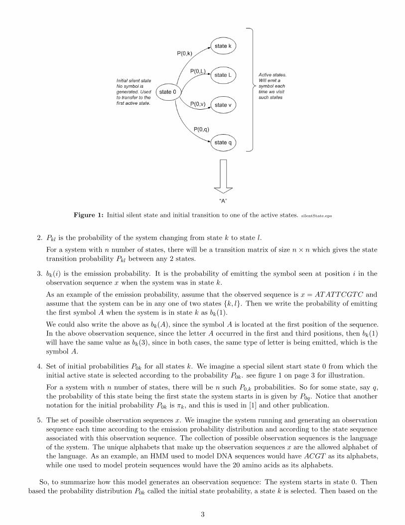
Figure 1: Initial silent state and initial transition to one of the active states. silentState.eps

2. Pkl is the probability of the system changing from state k to state l.

For a system with n number of states, there will be a transition matrix of size n× n which gives the statetransition probability Pkl between any 2 states.

3. bk(i) is the emission probability. It is the probability of emitting the symbol seen at position i in theobservation sequence x when the system was in state k.

As an example of the emission probability, assume that the observed sequence is x = ATATTCGTC andassume that the system can be in any one of two states {k, l}. Then we write the probability of emittingthe first symbol A when the system is in state k as bk(1).

We could also write the above as bk(A), since the symbol A is located at the first position of the sequence.In the above observation sequence, since the letter A occurred in the first and third positions, then bk(1)will have the same value as bk(3), since in both cases, the same type of letter is being emitted, which is thesymbol A.

4. Set of initial probabilities P0k for all states k. We imagine a special silent start state 0 from which theinitial active state is selected according to the probability P0k. see figure 1 on page 3 for illustration.

For a system with n number of states, there will be n such P0,k probabilities. So for some state, say q,the probability of this state being the first state the system starts in is given by P0q. Notice that anothernotation for the initial probability P0k is πk, and this is used in [1] and other publication.

5. The set of possible observation sequences x. We imagine the system running and generating an observationsequence each time according to the emission probability distribution and according to the state sequenceassociated with this observation sequence. The collection of possible observation sequences is the languageof the system. The unique alphabets that make up the observation sequences x are the allowed alphabet ofthe language. As an example, an HMM used to model DNA sequences would have ACGT as its alphabets,while one used to model protein sequences would have the 20 amino acids as its alphabets.

So, to summarize how this model generates an observation sequence: The system starts in state 0. Thenbased the probability distribution P0k called the initial state probability, a state k is selected. Then based on the

3

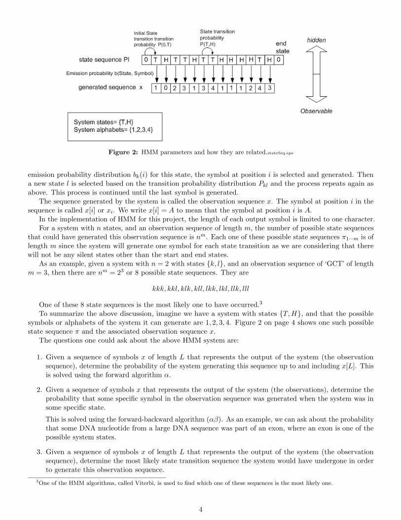
Figure 2: HMM parameters and how they are related.stateSeq.eps

emission probability distribution bk(i) for this state, the symbol at position i is selected and generated. Thena new state l is selected based on the transition probability distribution Pkl and the process repeats again asabove. This process is continued until the last symbol is generated.

The sequence generated by the system is called the observation sequence x. The symbol at position i in thesequence is called x[i] or xi. We write x[i] = A to mean that the symbol at position i is A.

In the implementation of HMM for this project, the length of each output symbol is limited to one character.For a system with n states, and an observation sequence of length m, the number of possible state sequences

that could have generated this observation sequence is nm. Each one of these possible state sequences π1···m is oflength m since the system will generate one symbol for each state transition as we are considering that therewill not be any silent states other than the start and end states.

As an example, given a system with n = 2 with states {k, l}, and an observation sequence of ‘GCT’ of lengthm = 3, then there are nm = 23 or 8 possible state sequences. They are

kkk, kkl, klk, kll, lkk, lkl, llk, lll

One of these 8 state sequences is the most likely one to have occurred.3

To summarize the above discussion, imagine we have a system with states {T,H}, and that the possiblesymbols or alphabets of the system it can generate are 1, 2, 3, 4. Figure 2 on page 4 shows one such possiblestate sequence π and the associated observation sequence x.

The questions one could ask about the above HMM system are:

1. Given a sequence of symbols x of length L that represents the output of the system (the observationsequence), determine the probability of the system generating this sequence up to and including x[L]. Thisis solved using the forward algorithm α.

2. Given a sequence of symbols x that represents the output of the system (the observations), determine theprobability that some specific symbol in the observation sequence was generated when the system was insome specific state.

This is solved using the forward-backward algorithm (αβ). As an example, we can ask about the probabilitythat some DNA nucleotide from a large DNA sequence was part of an exon, where an exon is one of thepossible system states.

3. Given a sequence of symbols x of length L that represents the output of the system (the observationsequence), determine the most likely state transition sequence the system would have undergone in orderto generate this observation sequence.

3One of the HMM algorithms, called Viterbi, is used to find which one of these sequences is the most likely one.

4

This is solved using the Viterbi algorithm γ. Note again that the sequence of states πi···j will have thesame length as the observation sequence xi···j .

The above problems are considered HMM analysis problems. There is another problem, which is the trainingor identification problem whose goal is to estimate the HMM parameters (the set of probabilities) we discussedon page 2 given some set of observation sequences taken from the type of data we wish to use the HMM toanalyze. As an example, to train the HMM for gene finding for the mouse genome, we would train the HMM ona set of sequences taken from this genome.

One standard algorithm used for HMM parameter estimation (or HMM training) is called Baum-Welch,and is a specialized algorithm of the more general algorithm called EM (for expectation maximization). In thecurrent MATLAB implementation, this algorithm is not implemented, but could be easily added later if timepermits.

A small observation: In these notations, and in the algorithms described below, I use the value 1 as the firstposition (or index) of any sequence instead of the more common 0 used in languages such as C, C++ or Java.This is only for ease of implementation as I will be using MATLAB for the implementation of these algorithms,and MATLAB uses 1 and not 0 as the starting index of an array. This made translating the algorithms intoMATALAB code much easier.

Graphical representations of an HMMThere are two main methods to graphically represent an HMM . One method shows the time axis (or the

position in the observation sequence) and the symbols emitted at each time instance (called the trellis diagram).The other method is a more concise way of representing the HMM, but does not show which symbol is emittedat what time instance.

To describe each representation, I will use an example, and show how the example can be representedgraphically in both methods.

1 Example HMM

Throughout this report, the following HMM example is used for illustration. The HMM configuration file for theexample that can be used with the current implementation is shown. Each different HMM state description(HMM parameters) is written in a plain text configuration file and read by the HMM implementation. Theformat of the HMM configuration file is described on page 15.

Assume the observed sequence is ATACC. This means that A was the first symbol emitted, seen at timet = 1, and T is the second symbol seen at time t = 2, and so forth. Notice that we imagine that the system willwrite out each symbol to the end of the current observation sequence.

Next, Assume the system can be in any one of two internal states {S, T}.Assume the state transition matrix Pkl to be as follows

PST = 0.3 PSS = 0.7

PTS = 0.4 PTT = 0.6

And for the initial probabilities P0k, assume the following

πS = 0.4

πT = 0.6

And finally for the emission probabilities bk(i), there are 3 unique symbols that are generated in this example(the alphabets of the language of the observation sequence), and they are A, T,C. So there will be 6 emissionprobabilities, 3 symbols for each state, and given we have 2 states, then we will have a total of 6 emissionprobabilities. Assume they are given by the following emission matrix:

bS(A) = 0.4 bS(C) = 0.4 bS(T ) = 0.2

bT (A) = 0.25 bT (C) = 0.55 bT (T ) = 0.2

5

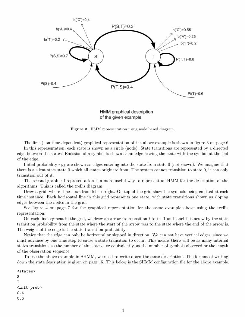
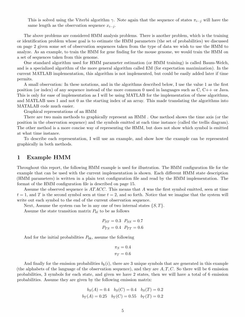
Figure 3: HMM representation using node based diagram.

The first (non-time dependent) graphical representation of the above example is shown in figure 3 on page 6In this representation, each state is shown as a circle (node). State transitions are represented by a directed

edge between the states. Emission of a symbol is shown as an edge leaving the state with the symbol at the endof the edge.

Initial probability π0,k are shown as edges entering into the state from state 0 (not shown). We imagine thatthere is a silent start state 0 which all states originate from. The system cannot transition to state 0, it can onlytransition out of it.

The second graphical representation is a more useful way to represent an HMM for the description of thealgorithms. This is called the trellis diagram.

Draw a grid, where time flows from left to right. On top of the grid show the symbols being emitted at eachtime instance. Each horizontal line in this grid represents one state, with state transitions shown as slopingedges between the nodes in the grid.

See figure 4 on page 7 for the graphical representation for the same example above using the trellisrepresentation.

On each line segment in the grid, we draw an arrow from position i to i+ 1 and label this arrow by the statetransition probability from the state where the start of the arrow was to the state where the end of the arrow is.The weight of the edge is the state transition probability.

Notice that the edge can only be horizontal or slopped in direction. We can not have vertical edges, since wemust advance by one time step to cause a state transition to occur. This means there will be as many internalstates transitions as the number of time steps, or equivalently, as the number of symbols observed or the lengthof the observation sequence.

To use the above example in SHMM, we need to write down the state description. The format of writingdown the state description is given on page 15. This below is the SHMM configuration file for the above example.

<states>

S

T

<init_prob>

0.4

0.6

6

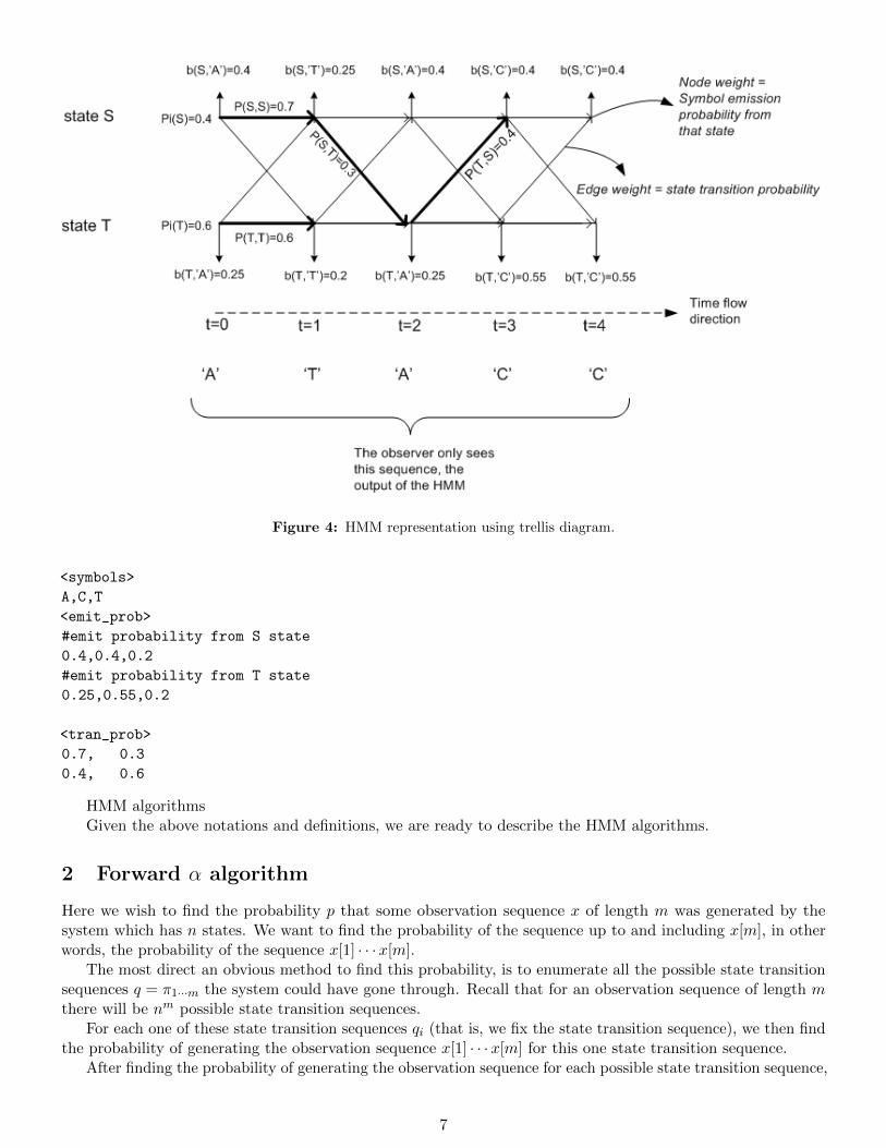
Figure 4: HMM representation using trellis diagram.

<symbols>

A,C,T

<emit_prob>

#emit probability from S state

0.4,0.4,0.2

#emit probability from T state

0.25,0.55,0.2

<tran_prob>

0.7, 0.3

0.4, 0.6

HMM algorithmsGiven the above notations and definitions, we are ready to describe the HMM algorithms.

2 Forward α algorithm

Here we wish to find the probability p that some observation sequence x of length m was generated by thesystem which has n states. We want to find the probability of the sequence up to and including x[m], in otherwords, the probability of the sequence x[1] · · ·x[m].

The most direct an obvious method to find this probability, is to enumerate all the possible state transitionsequences q = π1···m the system could have gone through. Recall that for an observation sequence of length mthere will be nm possible state transition sequences.

For each one of these state transition sequences qi (that is, we fix the state transition sequence), we then findthe probability of generating the observation sequence x[1] · · ·x[m] for this one state transition sequence.

After finding the probability of generating the observation sequence for each possible state transition sequence,

7

Figure 5: Finding the probability of a an observation sequence using brute search method.

Figure 6: Finding the probability of a sequence using the α method.

we sum all the resulting probabilities to obtain the probability of the observation sequence being generated bythe system.

As an example, for a system with states {S,K,Z} and observation sequence AGGT a partial list of thepossible state sequences we need to consider is shown in figure 5 on page 8.

We can perform the above algorithm as follows:Find the probability of the system emitting the symbol x[1] from π1. This is equal to the probability of

emitting the symbol x[1] from state π1 multiplied by the probability of being in state π1.Next, find the probability of generating the sequence x[1] · · ·x[2]. This is equal to the probability of emitting

the sequence x[1] (which we found from above), multiplied by the probability of moving from state π1 to stateπ2, multiplied by the probability of emitting the symbol x[2] from state π2.

Next, find the probability of generating the sequence x[1] · · ·x[3]. This is equal to the probability of emittingthe sequence x[1] · · ·x[2] (which we found from above), multiplied by the probability of moving from state π2 tostate π3, multiplied by the probability of emitting the symbol x[3] from state π3.

We continue until we find the probability of emitting the full sequence x[1] · · ·x[m]Obviously the above algorithm is not efficient. There are nm possible state sequences, and for each one we

have to perform O(2m) multiplications, resulting in O(m nm) multiplications in total.For an observation sequence of length m = 500 and a system with n = 10 states, we have to wait a very long

time for this computation to complete.A much improved method is the α algorithm. The idea of the α algorithm, is that instead of finding the

probability for each different state sequence separately and then summing the resulting probabilities, we scan thesequence x[1] · · ·x[i] from left to right, one position at a time, but for each position we calculate the probabilityof generating the sequence up to this position for all the possible states.

Let us call the probability of emitting the sequence x[1] · · ·x[i] as α(i). And we call the probability ofemitting x[1] · · ·x[i] when the system was in state k when emitting x[i] as αk(i).

So, the probability of emitting the sequence x[1] · · ·x[i] will be equal to the probability of emitting the samesequence but with x[i] being emitted from one state say k, this is called αk(i), plus the probability of emittingthe same sequence but with x[i] being emitted from another state, say l, this is called αl(i), and so forth untilwe have covered all the possible states. In other words α(i) is the

∑k αk(i) for all states k.

Each αk(i) is found by multiplying the α(i− 1) for each of the states, by the probability of moving from eachof those states to state k, multiplied by the probability of emitting x[i] from state k. This step is illustrated infigure 6 on page 8.

Each time we calculate αk(i) for some state k, we store this value, and use it when calculating α(i + 1).

8

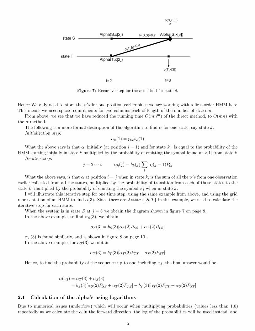
Figure 7: Recursive step for the α method for state S.

Hence We only need to store the α′s for one position earlier since we are working with a first-order HMM here.This means we need space requirements for two columns each of length of the number of states n.

From above, we see that we have reduced the running time O(mnm) of the direct method, to O(mn) withthe α method.

The following is a more formal description of the algorithm to find α for one state, say state k.Initialization step:

αk(1) = p0kbk(1)

What the above says is that α, initially (at position i = 1) and for state k , is equal to the probability of theHMM starting initially in state k multiplied by the probability of emitting the symbol found at x[1] from state k.

Iterative step:

j = 2 · · · i αk(j) = bk(j)∑l

αl(j − 1)Plk

What the above says, is that α at position i = j when in state k, is the sum of all the α′s from one observationearlier collected from all the states, multiplied by the probability of transition from each of those states to thestate k, multiplied by the probability of emitting the symbol xj when in state k.

I will illustrate this iterative step for one time step, using the same example from above, and using the gridrepresentation of an HMM to find α(3). Since there are 2 states {S, T} in this example, we need to calculate theiterative step for each state.

When the system is in state S at j = 3 we obtain the diagram shown in figure 7 on page 9.In the above example, to find αS(3), we obtain

αS(3) = bS(3)[αS(2)PSS + αT (2)PTS ]

αT (3) is found similarly, and is shown in figure 8 on page 10.In the above example, for αT (3) we obtain

αT (3) = bT (3)[αT (2)PTT + αS(2)PST ]

Hence, to find the probability of the sequence up to and including x3, the final answer would be

α(x3) = αT (3) + αS(3)

= bS(3)[αS(2)PSS + αT (2)PTS ] + bT (3)[αT (2)PTT + αS(2)PST ]

2.1 Calculation of the alpha’s using logarithms

Due to numerical issues (underflow) which will occur when multiplying probabilities (values less than 1.0)repeatedly as we calculate the α in the forward direction, the log of the probabilities will be used instead, and

9

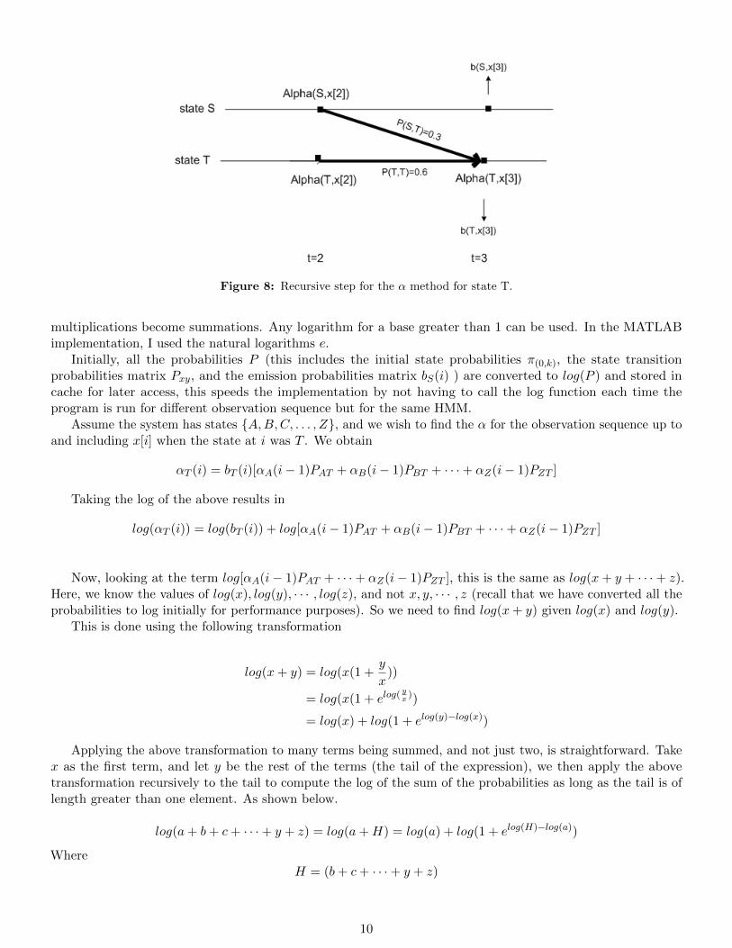
Figure 8: Recursive step for the α method for state T.

multiplications become summations. Any logarithm for a base greater than 1 can be used. In the MATLABimplementation, I used the natural logarithms e.

Initially, all the probabilities P (this includes the initial state probabilities π(0,k), the state transitionprobabilities matrix Pxy, and the emission probabilities matrix bS(i) ) are converted to log(P ) and stored incache for later access, this speeds the implementation by not having to call the log function each time theprogram is run for different observation sequence but for the same HMM.

Assume the system has states {A,B,C, . . . , Z}, and we wish to find the α for the observation sequence up toand including x[i] when the state at i was T . We obtain

αT (i) = bT (i)[αA(i− 1)PAT + αB(i− 1)PBT + · · ·+ αZ(i− 1)PZT ]

Taking the log of the above results in

log(αT (i)) = log(bT (i)) + log[αA(i− 1)PAT + αB(i− 1)PBT + · · ·+ αZ(i− 1)PZT ]

Now, looking at the term log[αA(i− 1)PAT + · · ·+ αZ(i− 1)PZT ], this is the same as log(x+ y + · · ·+ z).Here, we know the values of log(x), log(y), · · · , log(z), and not x, y, · · · , z (recall that we have converted all theprobabilities to log initially for performance purposes). So we need to find log(x+ y) given log(x) and log(y).

This is done using the following transformation

log(x+ y) = log(x(1 +y

x))

= log(x(1 + elog(yx))

= log(x) + log(1 + elog(y)−log(x))

Applying the above transformation to many terms being summed, and not just two, is straightforward. Takex as the first term, and let y be the rest of the terms (the tail of the expression), we then apply the abovetransformation recursively to the tail to compute the log of the sum of the probabilities as long as the tail is oflength greater than one element. As shown below.

log(a+ b+ c+ · · ·+ y + z) = log(a+H) = log(a) + log(1 + elog(H)−log(a))

WhereH = (b+ c+ · · ·+ y + z)

10

Now repeat the above process to find log(b+ c+ · · ·+ y + z).

log(b+ c+ · · ·+ y + z) = log(b+H) = log(b) + log(1 + elog(H)−log(b))

Where now H = (c+ · · ·+ y + z).Continue the above recursive process, until the expression H contains one term to obtain

log(y + z) = log(y) + log(1 + elog(z)−log(y))

This is a sketch of a function which accomplishes the above.

function Log_Of_Sums(A: array 1..n of probabilities) returns double IS

begin

IF (length(A)>2) THEN

return( log(A[1]) + log( 1 + exp( Log_of_Sums(A[2..n])) - log( A[1] )));

ELSE

return( log(A[1] + log( 1 + exp( A[2] - log( A[1] )));

END

end log_Of_Sums

The number of states is usually much less than the number of observations, so there is no problems (such asstack overflow issues) with using recursion in this case.

3 Backward β algorithm

Here we are interested in finding the probability that some part of the sequence was generated when the systemwas in some specific state.

For example, we might want to find, looking at a DNA sequence x, the probability that some nucleotide atsome position, say x[i] was generated from an exon, where an exon is one of the possible states the system canbe in.

Let such state be S. Let the length of the sequence be L, then we need to obtain P (πi = S|xi...L). In thefollowing, when x is written without subscripts, it is understood to stand for the whole sequence x1 · · ·xL. Alsoxi is the same as x[i].

Using Baye’s probability rule we get

P (πi = S|x) = P (πi = S, x)

P (x)

But the joint probability P (πi = S, x) can be found from

P (πi = S, x) = P (x1 · · ·xi, πi = S)P (xi+1 · · ·xL|πi = S)

Looking at the equation above, we see that P (x1 . . . xi, πi = S) is nothing but αS(i), which is defined as theprobability of the sequence x1 · · ·xi with x[i] being generated from state S.

The second quantity P (xi+1 · · ·xL|πi = S) is found using the backward β algorithm as described below.Initialization step:For each state k, let βk(L) = 1recursive step:

i = (L− 1) · · · 1 βk(i) =∑l

Pklbl(i+ 1)βl(i+ 1)

Where the sum above is done over all states. Hence

P (πi = S|x) = αS(i)βS(i)

P (x)

11

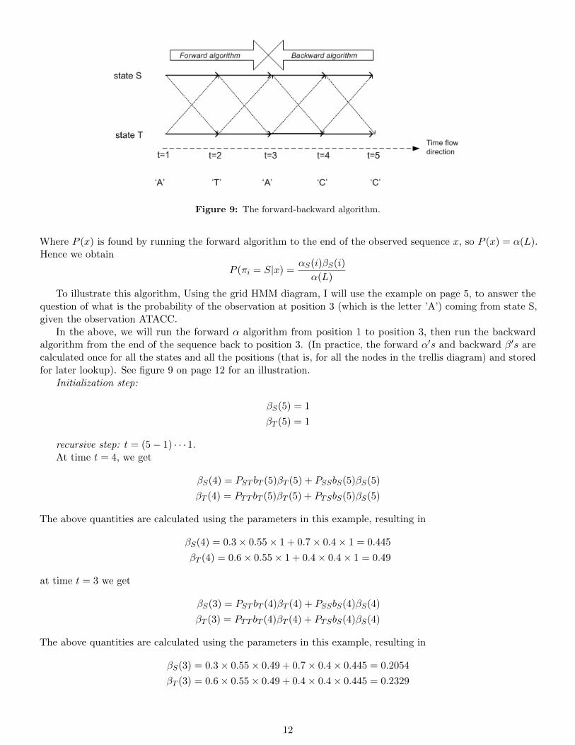
Figure 9: The forward-backward algorithm.

Where P (x) is found by running the forward algorithm to the end of the observed sequence x, so P (x) = α(L).Hence we obtain

P (πi = S|x) = αS(i)βS(i)

α(L)

To illustrate this algorithm, Using the grid HMM diagram, I will use the example on page 5, to answer thequestion of what is the probability of the observation at position 3 (which is the letter ’A’) coming from state S,given the observation ATACC.

In the above, we will run the forward α algorithm from position 1 to position 3, then run the backwardalgorithm from the end of the sequence back to position 3. (In practice, the forward α′s and backward β′s arecalculated once for all the states and all the positions (that is, for all the nodes in the trellis diagram) and storedfor later lookup). See figure 9 on page 12 for an illustration.

Initialization step:

βS(5) = 1

βT (5) = 1

recursive step: t = (5− 1) · · · 1.At time t = 4, we get

βS(4) = PST bT (5)βT (5) + PSSbS(5)βS(5)

βT (4) = PTT bT (5)βT (5) + PTSbS(5)βS(5)

The above quantities are calculated using the parameters in this example, resulting in

βS(4) = 0.3× 0.55× 1 + 0.7× 0.4× 1 = 0.445

βT (4) = 0.6× 0.55× 1 + 0.4× 0.4× 1 = 0.49

at time t = 3 we get

βS(3) = PST bT (4)βT (4) + PSSbS(4)βS(4)

βT (3) = PTT bT (4)βT (4) + PTSbS(4)βS(4)

The above quantities are calculated using the parameters in this example, resulting in

βS(3) = 0.3× 0.55× 0.49 + 0.7× 0.4× 0.445 = 0.2054

βT (3) = 0.6× 0.55× 0.49 + 0.4× 0.4× 0.445 = 0.2329

12

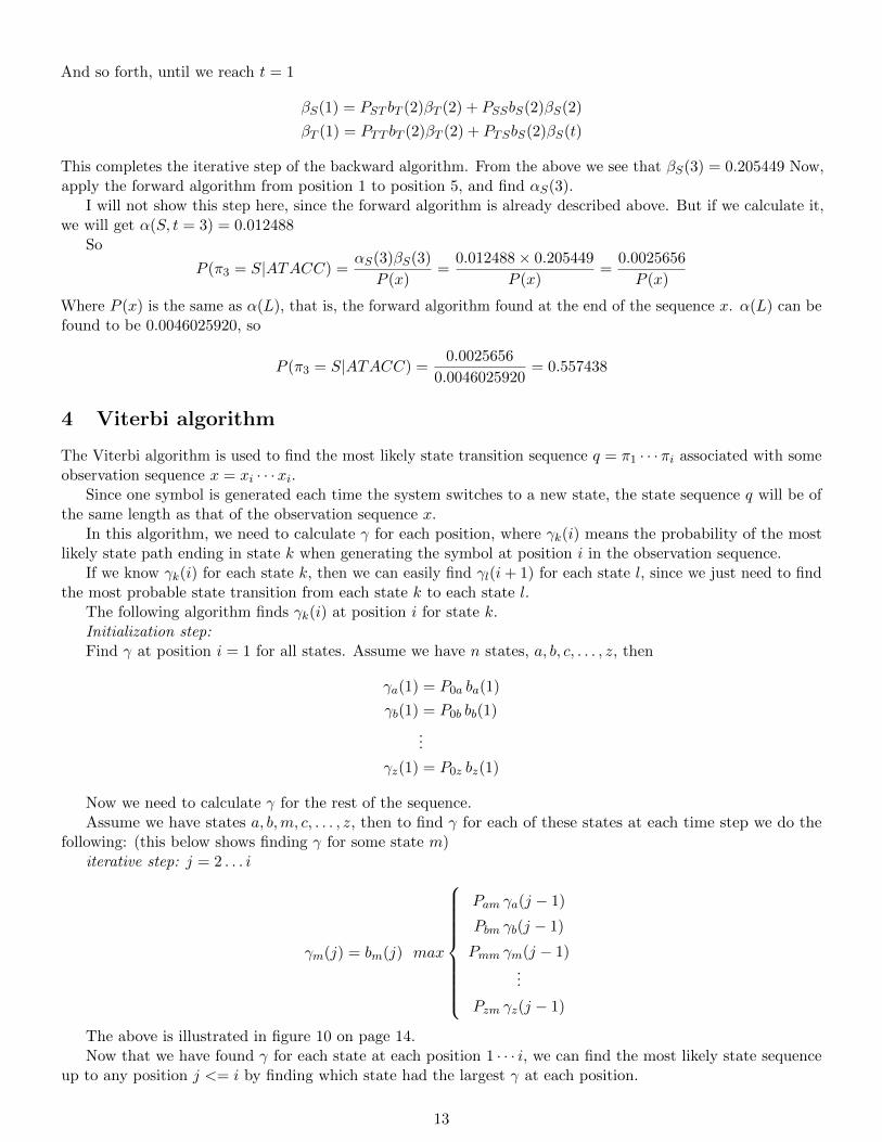
And so forth, until we reach t = 1

βS(1) = PST bT (2)βT (2) + PSSbS(2)βS(2)

βT (1) = PTT bT (2)βT (2) + PTSbS(2)βS(t)

This completes the iterative step of the backward algorithm. From the above we see that βS(3) = 0.205449 Now,apply the forward algorithm from position 1 to position 5, and find αS(3).

I will not show this step here, since the forward algorithm is already described above. But if we calculate it,we will get α(S, t = 3) = 0.012488

So

P (π3 = S|ATACC) =αS(3)βS(3)

P (x)=

0.012488× 0.205449

P (x)=

0.0025656

P (x)

Where P (x) is the same as α(L), that is, the forward algorithm found at the end of the sequence x. α(L) can befound to be 0.0046025920, so

P (π3 = S|ATACC) =0.0025656

0.0046025920= 0.557438

4 Viterbi algorithm

The Viterbi algorithm is used to find the most likely state transition sequence q = π1 · · ·πi associated with someobservation sequence x = xi · · ·xi.

Since one symbol is generated each time the system switches to a new state, the state sequence q will be ofthe same length as that of the observation sequence x.

In this algorithm, we need to calculate γ for each position, where γk(i) means the probability of the mostlikely state path ending in state k when generating the symbol at position i in the observation sequence.

If we know γk(i) for each state k, then we can easily find γl(i+ 1) for each state l, since we just need to findthe most probable state transition from each state k to each state l.

The following algorithm finds γk(i) at position i for state k.Initialization step:Find γ at position i = 1 for all states. Assume we have n states, a, b, c, . . . , z, then

γa(1) = P0a ba(1)

γb(1) = P0b bb(1)

...

γz(1) = P0z bz(1)

Now we need to calculate γ for the rest of the sequence.Assume we have states a, b,m, c, . . . , z, then to find γ for each of these states at each time step we do the

following: (this below shows finding γ for some state m)iterative step: j = 2 . . . i

γm(j) = bm(j) max

Pam γa(j − 1)

Pbm γb(j − 1)

Pmm γm(j − 1)...

Pzm γz(j − 1)

The above is illustrated in figure 10 on page 14.Now that we have found γ for each state at each position 1 · · · i, we can find the most likely state sequence

up to any position j <= i by finding which state had the largest γ at each position.

13

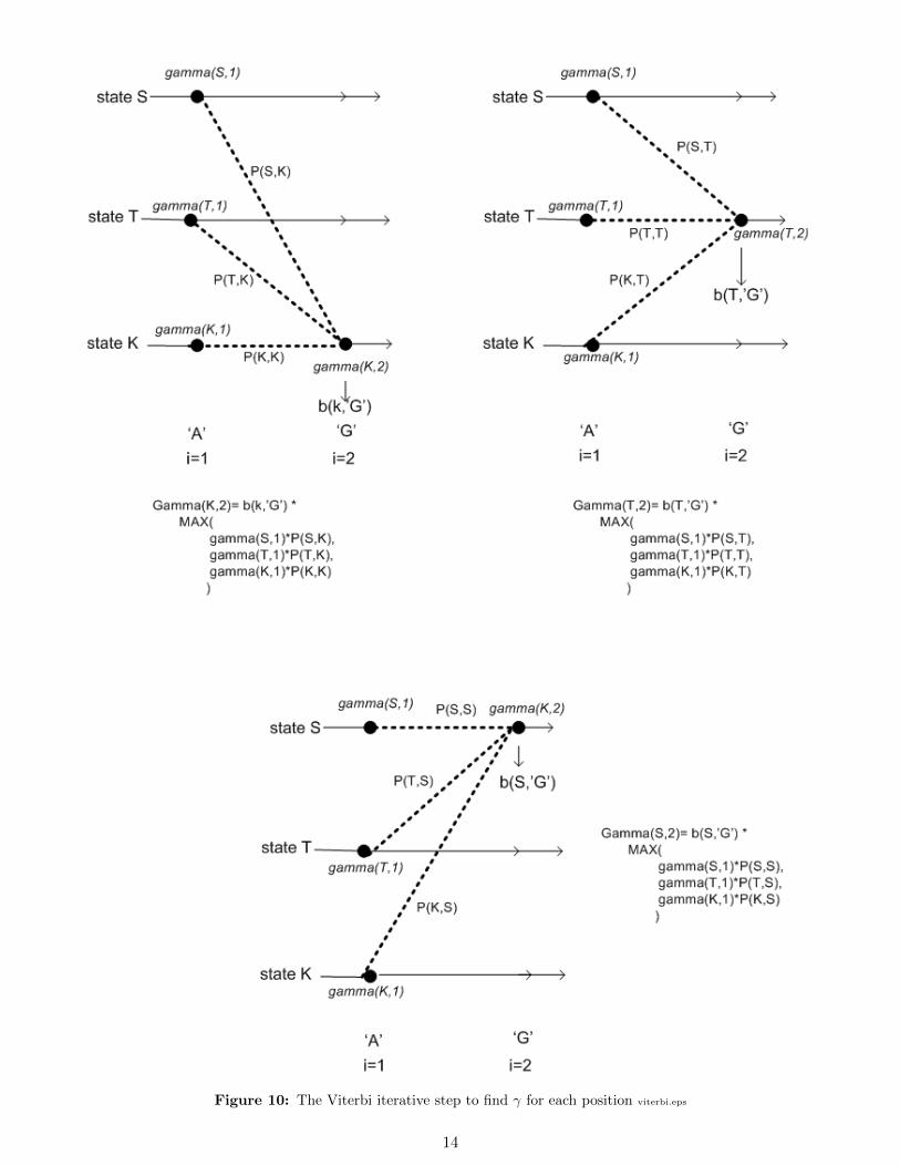
Figure 10: The Viterbi iterative step to find γ for each position viterbi.eps

14

Design and user guide of SHMMTo help understand HMMs more, I have implemented, in MATLAB, a basic HMM with a GUI user interface

for ease of use. This tool accepts an HMM description (model parameters) from a plain text configuration file.The tool (called SHMM, for simple HMM) implements the forward, backward, and Viterbi algorithms. Thisimplementation is for a first order HMM model.

Due to lack of time to implement an HMM for an order greater than a first order, which is needed toenable this tool to be used for such problems as gene finding (to detect splice sites, start of exon, etc. . . ). Thisimplementation therefor is restricted to one character look-ahead on the observation sequence. However, evenwith this limitation, this tool can be useful for learning how HMM’s work.

SHMM takes as input a plain text configuration file (default .hmm extension), which contains the descriptionof the HMM (states, initial probabilities, emission probabilities, symbols and transition probabilities). And theuser is asked to type in the observation sequence in a separate window for analysis.

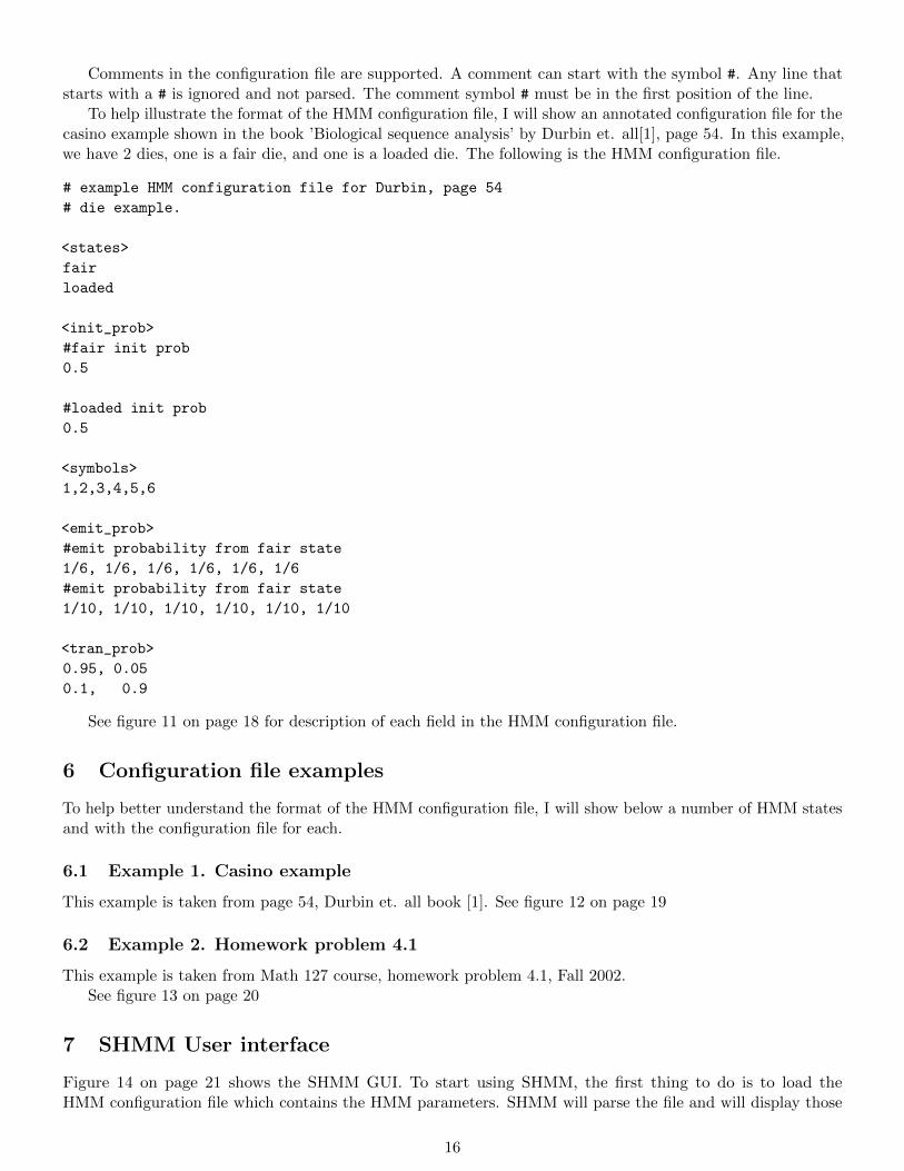
5 Configuration file description

The configuration file is broken into 5 sections. The order of the sections must be as shown below. All 5 sectionsmust exist. Each section starts with the name of the section, contained inside a left < and a right > brackets.No space is allowed after < or before >. The entries in the file are case sensitive. So a state called ’sunny’ willbe taken as different from a state called ’SUNNY’. The same applies to the characters allowed in the observationsequence: the letter ’g’ is taken as different from ’G’.

The sections, and the order in which they appear in the configuration file, must be as this, from top tobottom:

1. <states>

2. <init_prob>

3. <symbols>

4. <emit_prob>

5. <tran_prob>

In the <states> sections, the names of the states are listed. One name per line. Names must not contain aspace.

In the <init_prob> section, the initial probabilities of being in each state are listed. One per line. Onenumber per line. The order of the states is assumed the same as the order in the <states> section. This meansthe initial probability of being in the first state listed in the <states> section will be assumed to be the firstnumber in the <init_prob> section.

In the <symbols> section, the observation symbols are listed. Each symbol must be one character long,separated by a comma. Can use as many lines as needed to list all the symbols. The symbol must be analphanumeric character.

In the <emit_prob> section, we list the probability of emitting each symbol from each state. The order ofthe states is assumed to be the same order of the states as in the <states> section.

The emission probability for each symbol is read. The order of the symbols is taken as the same order shownin the symbols section. The emission probabilities are separated by a comma. One line per state. See examplesbelow.

In the <tran_prob>, we list the transition probability matrix. This is the probability of changing state fromeach state to another. One line represent one row in the matrix. Entries are separated by a comma. One rowmust occupy one line only. The order of the rows is the same as the order of the states shown in the <states>section.

For example, if we have 2 states S1,S2, then the first line will be the row that represents S1->S1, and S1->S2

transition probabilities. Where S1->S1 is in position 1,1 of matrix, and S1->S2 will be in position 1,2 in thematrix. See example below for illustration.

15

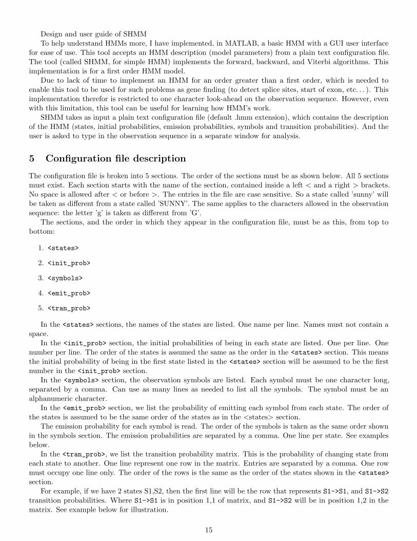
Comments in the configuration file are supported. A comment can start with the symbol #. Any line thatstarts with a # is ignored and not parsed. The comment symbol # must be in the first position of the line.

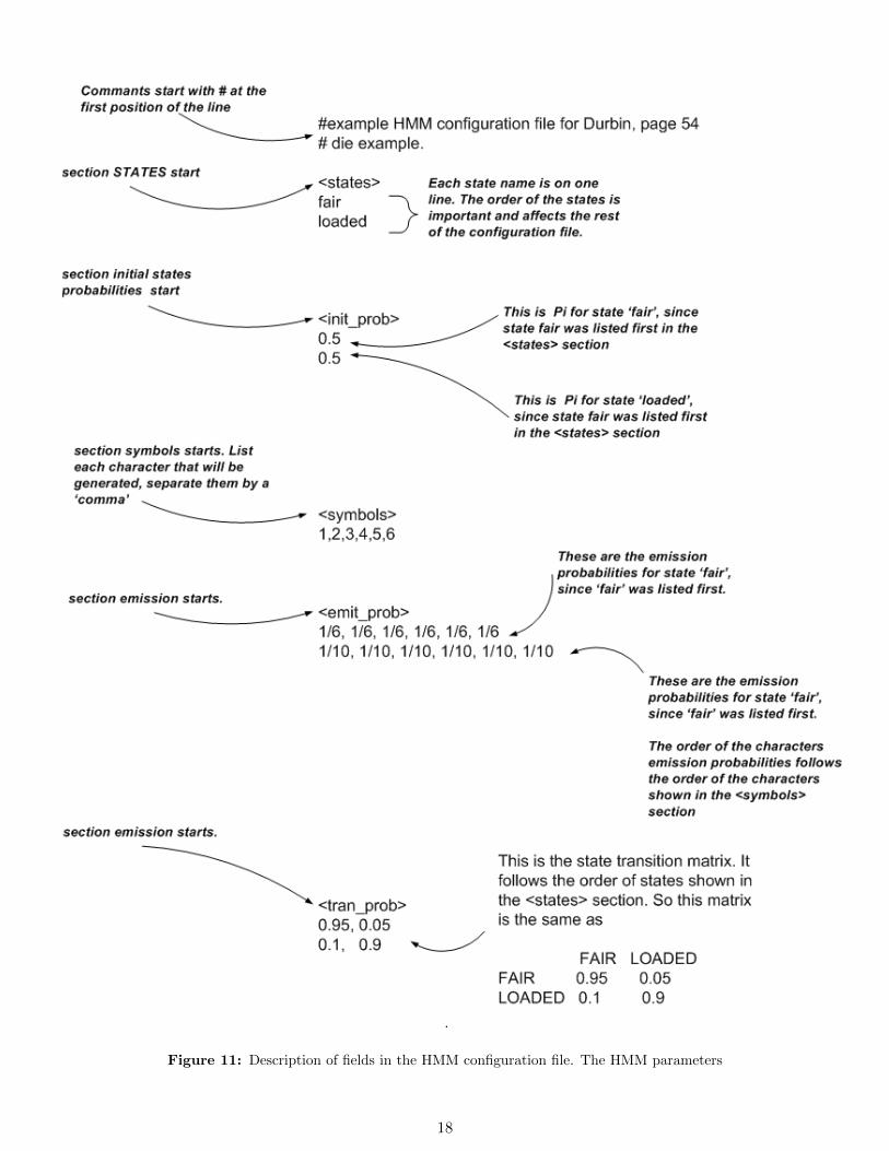
To help illustrate the format of the HMM configuration file, I will show an annotated configuration file for thecasino example shown in the book ’Biological sequence analysis’ by Durbin et. all[1], page 54. In this example,we have 2 dies, one is a fair die, and one is a loaded die. The following is the HMM configuration file.

# example HMM configuration file for Durbin, page 54

# die example.

<states>

fair

loaded

<init_prob>

#fair init prob

0.5

#loaded init prob

0.5

<symbols>

1,2,3,4,5,6

<emit_prob>

#emit probability from fair state

1/6, 1/6, 1/6, 1/6, 1/6, 1/6

#emit probability from fair state

1/10, 1/10, 1/10, 1/10, 1/10, 1/10

<tran_prob>

0.95, 0.05

0.1, 0.9

See figure 11 on page 18 for description of each field in the HMM configuration file.

6 Configuration file examples

To help better understand the format of the HMM configuration file, I will show below a number of HMM statesand with the configuration file for each.

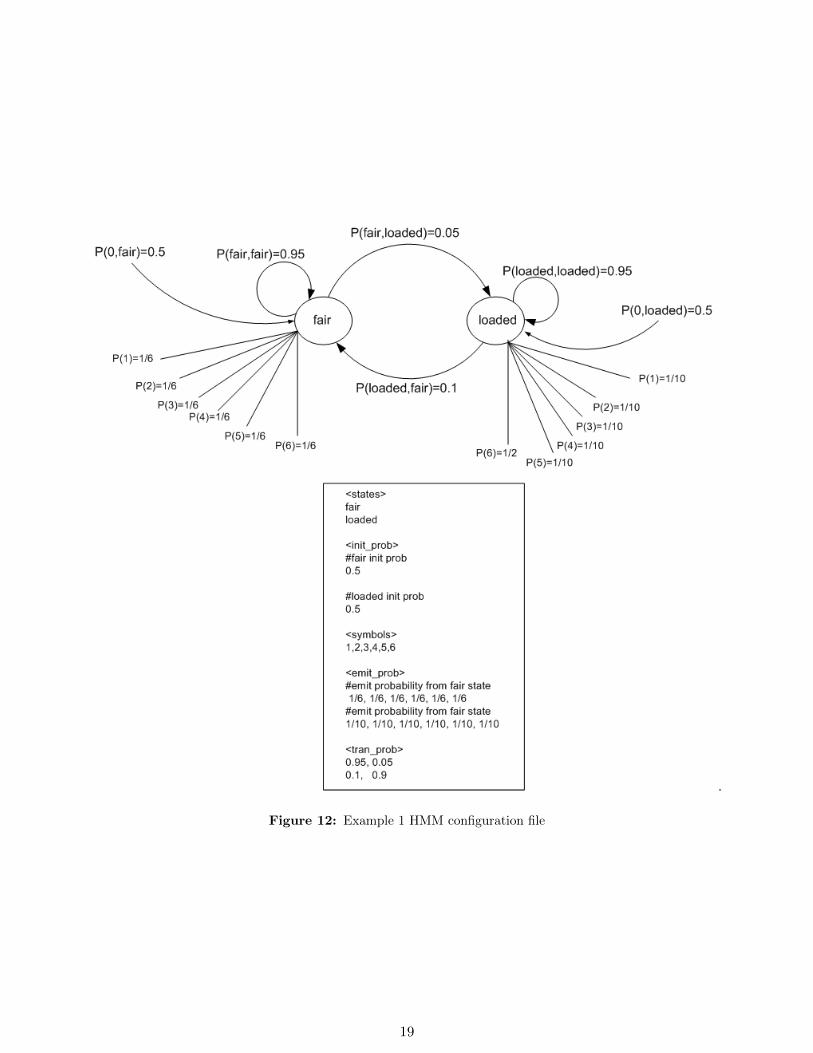
6.1 Example 1. Casino example

This example is taken from page 54, Durbin et. all book [1]. See figure 12 on page 19

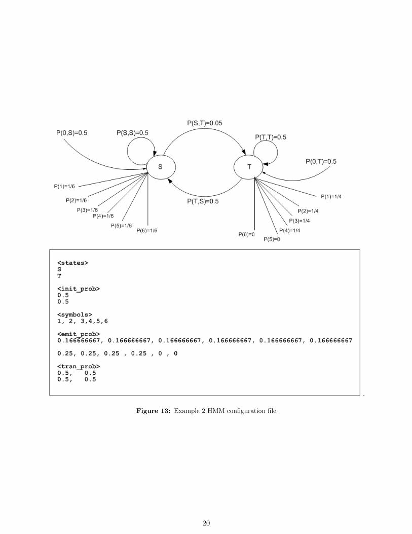
6.2 Example 2. Homework problem 4.1

This example is taken from Math 127 course, homework problem 4.1, Fall 2002.See figure 13 on page 20

7 SHMM User interface

Figure 14 on page 21 shows the SHMM GUI. To start using SHMM, the first thing to do is to load theHMM configuration file which contains the HMM parameters. SHMM will parse the file and will display those

16

parameters. Next, type into the observation sequence window the observation sequence itself. This sequencecould be cut and pasted into the window as well. Spaces and new lines are ignored.

Next, hit the top right RUN button. This will cause SHMM to evaluate the α, β and γ for each node in thetrellis diagram, and will display all these values. For the γ calculations, the nodes in the trellis diagram whichare on the Viterbi path have a ‘*’ next to them.

To invoke the (α, β) algorithm, enter the position in the observation and the state name and hit the smallRUN button inside the window titled Alpha Beta.

To modify the HMM parameters and run SHMM again, simply use an outside editor to do the changes inthe HMM configuration file, then load the file again into SHMM using the ‘Open’ button.

8 Source code description

The following is a list of all the MATLAB files that make up SHMM, with a brief description of each file. At theend of this report is the source code listing.

• nma hmmGUI.fig: The binary description of the GUI itself. It is automatically generated by MATLABusing GUIDE.

• nma hmmGUI.m: The MATLAB code that contains the properties of each component in the GUI.

• nma hmm main.m: This is the main function, which loads the GUI and initializes SHMM.

• nma hmm callbacks.m: The callbacks which are called when the user activate any control on the GUI.

• nma readHMM.m:

• nma hmmBackward.m: The function which calculates β.

• nma hmmForward.m: The function which calculates α.

• nma hmm veterbi.m: The function which calculates γ.

• nma hmmEmitProb.m: A utility function which returns the emission probability given a symbol and astate.

• nma trim.m: A utility function which removes leading and trailing spaces from a string.

• getPosOfState.m: A utility function which returns position of state in an array given the state name.

• nma logOfSums.m: A utility function which calculates the log of sum of logs for the α computation.

• nma logOfSumsBeta.m: A utility function which calculates the log of sum of logs for the β computation.

9 Installation instructions

Included on the CDROM are 2 files: setup.exe and unix.tar. The file setup.exe is the installer for windows.On windows, simply double click the file setup.exe and follow the instructions. When installation is completed,an icon will be created on the desktop called MATH127. Double click on this icon to open. Then 2 icons willappear. One of them is titled HMM. Double click on that to start SHMM. A GUI will appear.

On Unix (Linux or Solaris), no installer is supplied. Simply untar the file math127.zip. This will createthe same tree that the installer would create on windows. The tree contains a folder called src, which containsthe source code needed to run SHMM from inside matlab. To run SHMM on Unix, cd to the folder where youuntarred the file math127.tar, which will be called MATH127 by default, and navigate to the src folder for theHMM project. Then run the file nma hmm main from inside MATLAB console to start SHMM.

This report is in .ps format, and the original .tex file and the diagram files are included in the doc folder.Example HMM configuration files for use with SHMM are included in the conf folder.

17

.

Figure 11: Description of fields in the HMM configuration file. The HMM parameters

18

.

Figure 12: Example 1 HMM configuration file

19

.

Figure 13: Example 2 HMM configuration file

20

.

Figure 14: SHMM MATLAB user interface

21

References

[1] R.Durbin,S.Eddy,A.Krogh,G.Mitchison. Biological Sequence Analysis.

[2] Dr Lior Pachter lecture notes. Math 127. Fall 2002. UC Berkeley.

[3] Identification of genes in human genomic DNA. By Christopher Burge, Stanford University, 1997.

22