I529: Machine Learning in Bioinformatics (Spring 2013)

Hidden Markov Models

Yuzhen Ye School of Informatics and Computing

Indiana University, Bloomington Spring 2013

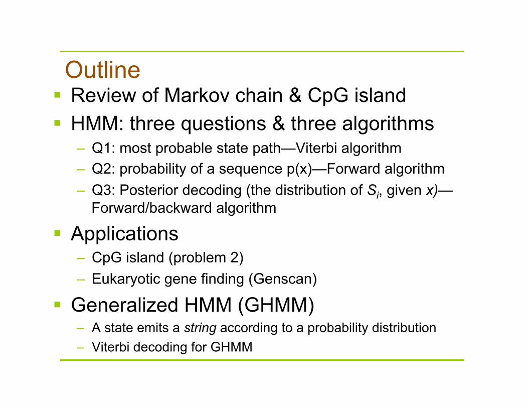
Outline   Review of Markov chain & CpG island   HMM: three questions & three algorithms

–  Q1: most probable state path—Viterbi algorithm –  Q2: probability of a sequence p(x)—Forward algorithm –  Q3: Posterior decoding (the distribution of Si, given x)—

Forward/backward algorithm

  Applications –  CpG island (problem 2) –  Eukaryotic gene finding (Genscan)

  Generalized HMM (GHMM) –  A state emits a string according to a probability distribution –  Viterbi decoding for GHMM

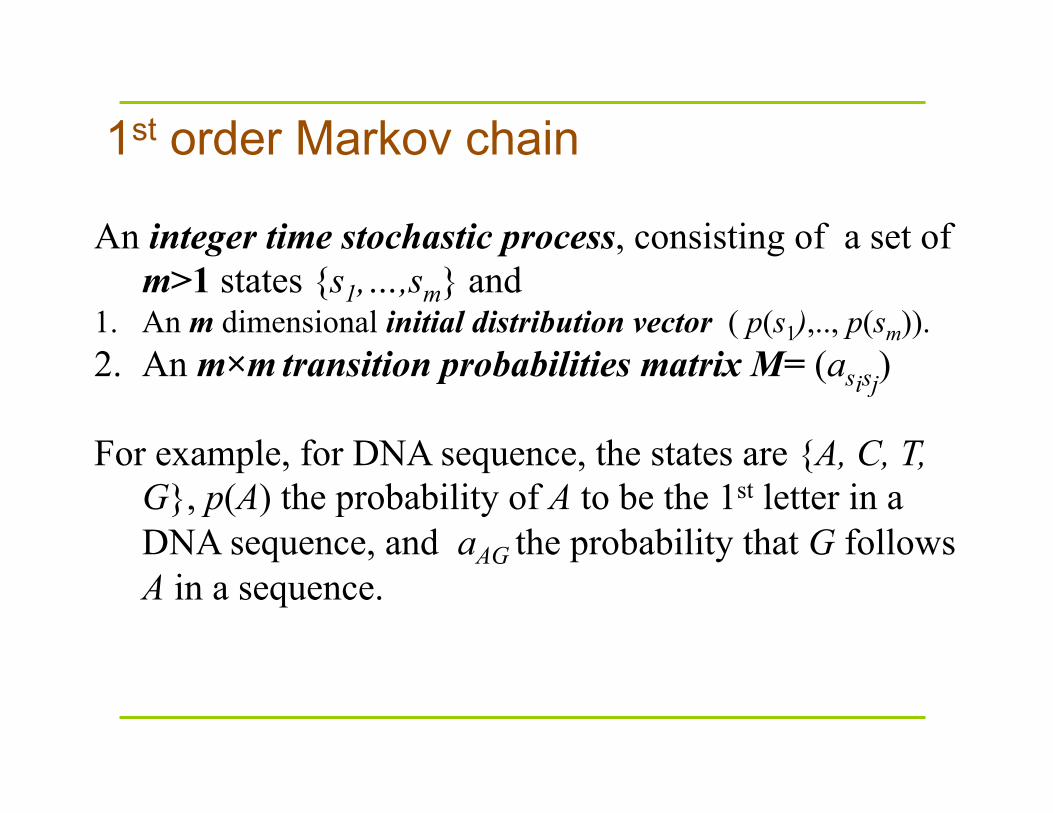
1st order Markov chain

An integer time stochastic process, consisting of a set of m>1 states {s1,…,sm} and

1.  An m dimensional initial distribution vector ( p(s1),.., p(sm)). 2.  An m×m transition probabilities matrix M= (asisj) For example, for DNA sequence, the states are {A, C, T,

G}, p(A) the probability of A to be the 1st letter in a DNA sequence, and aAG the probability that G follows A in a sequence.

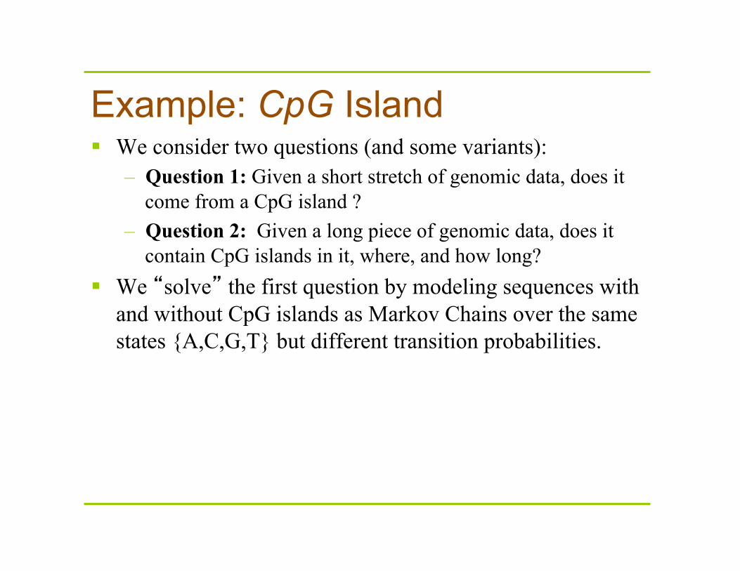
Example: CpG Island   We consider two questions (and some variants):

–  Question 1: Given a short stretch of genomic data, does it come from a CpG island ?

–  Question 2: Given a long piece of genomic data, does it contain CpG islands in it, where, and how long?

  We “solve” the first question by modeling sequences with and without CpG islands as Markov Chains over the same states {A,C,G,T} but different transition probabilities.

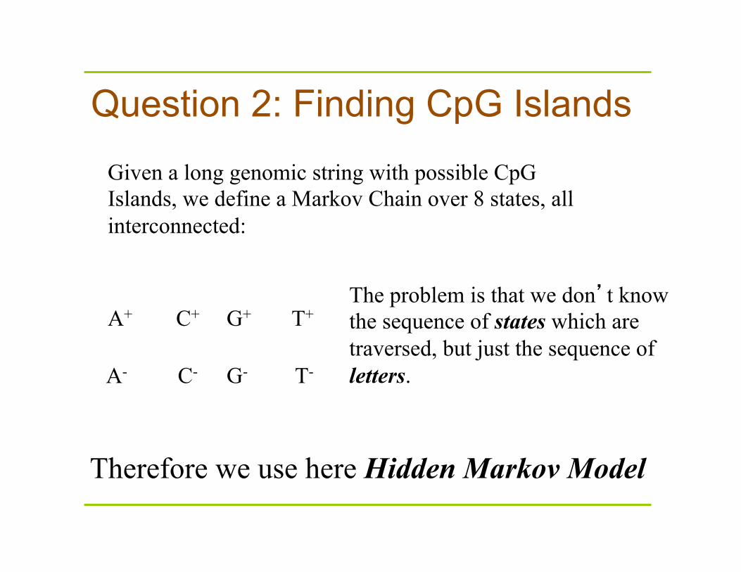
Question 2: Finding CpG Islands

Given a long genomic string with possible CpG Islands, we define a Markov Chain over 8 states, all interconnected:

C+ T+ G+ A+

C- T- G- A-

The problem is that we don’t know the sequence of states which are traversed, but just the sequence of letters.

Therefore we use here Hidden Markov Model

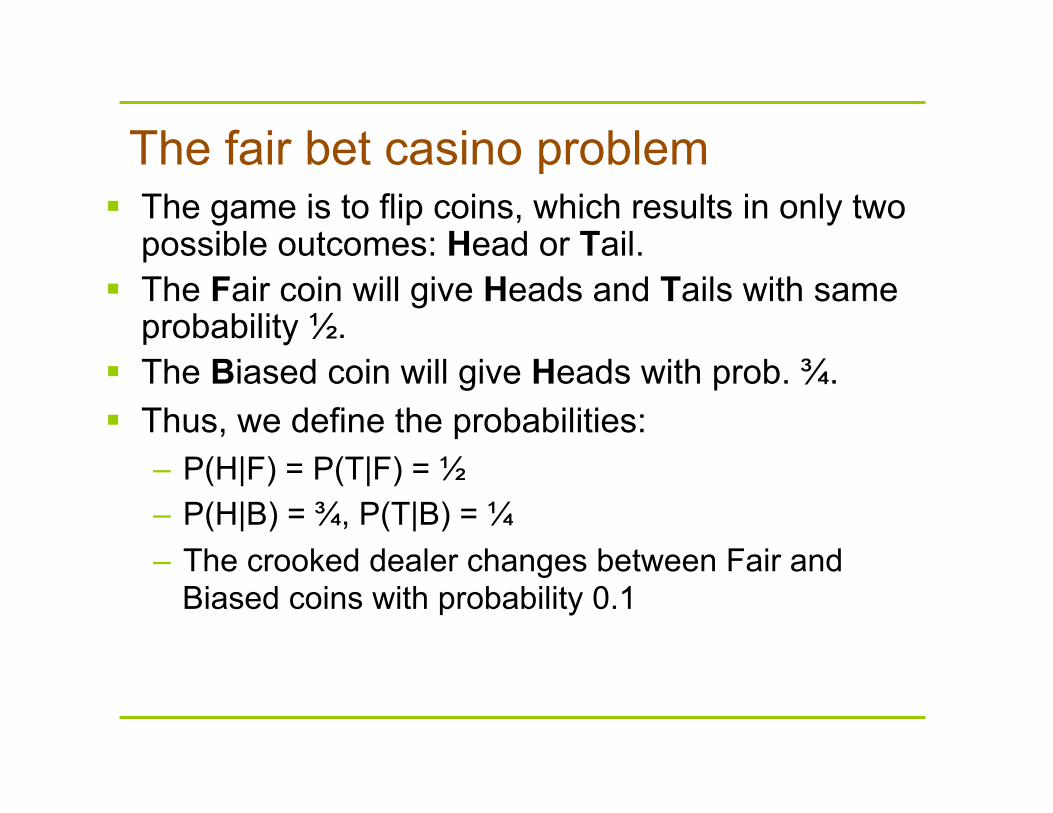
The fair bet casino problem   The game is to flip coins, which results in only two

possible outcomes: Head or Tail.   The Fair coin will give Heads and Tails with same

probability ½.   The Biased coin will give Heads with prob. ¾.   Thus, we define the probabilities:

–  P(H|F) = P(T|F) = ½ –  P(H|B) = ¾, P(T|B) = ¼ –  The crooked dealer changes between Fair and

Biased coins with probability 0.1

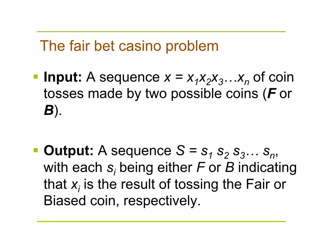
The fair bet casino problem

  Input: A sequence x = x1x2x3…xn of coin tosses made by two possible coins (F or B).

 Output: A sequence S = s1 s2 s3… sn,

with each si being either F or B indicating that xi is the result of tossing the Fair or Biased coin, respectively.

Hidden Markov model (HMM) •  Can be viewed as an abstract machine with k

hidden states that emits symbols from an alphabet Σ.

•  Each state has its own probability distribution, and the machine switches between states according to this probability distribution.

•  While in a certain state, the machine makes 2 decisions: – What state should I move to next? – What symbol - from the alphabet Σ - should I

emit?

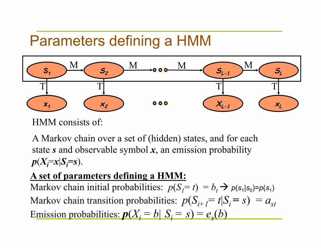
Parameters defining a HMM

A Markov chain over a set of (hidden) states, and for each state s and observable symbol x, an emission probability p(Xi=x|Si=s).

S1 S2 SL-1 SL

x1 x2 XL-1 xL

M M M M

T T T T

A set of parameters defining a HMM: Markov chain initial probabilities: p(S1= t) = bt p(s1|s0)=p(s1) Markov chain transition probabilities: p(Si+1= t|Si = s) = ast Emission probabilities: p(Xi = b| Si = s) = es(b)

HMM consists of:

Why “hidden”?

  Observers can see the emitted symbols of an HMM but have no ability to know which state the HMM is currently in.

  Thus, the goal is to infer the most likely hidden states of an HMM based on the given sequence of emitted symbols.

Question 2: Given a long piece of genomic data, does it contain CpG islands in it, where, and how long? Hidden Markov Model: this seems a straightforward model (but we will discuss later why this model is NOT good). Hidden states: {‘+’, ‘-’} Observable symbols: {A, C, G, T}

Example: CpG island

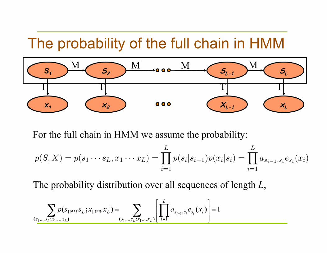
The probability of the full chain in HMM

S1 S2 SL-1 SL

x1 x2 XL-1 xL

M M M M

T T T T

For the full chain in HMM we assume the probability:

The probability distribution over all sequences of length L,

111

1

11 111 =

⎥⎥⎦

⎤

⎢⎢⎣

⎡= ∑ ∏∑

=−

),..,;,..,(,

),..,;,..,(

)(),..,;,..,(LL

iii

LL xxss

L

iisss

xxssLL xeaxxssp

Templates for equations

Yuzhen Ye

January 21, 2013

1 Equation for slides

HMM

p(S,X) = p(s1 · · · sL, x1 · · ·xL) =LY

i=1

p(si|si�1)p(xi|si) =LY

i=1

asi�1,siesi(xi) (1)

Simple models for gene prediction:

P (c|GC%) =P (GC%|c)P (c)

P (GC%)=

P (GC%|c)P (c)

P (GC%|c)P (c) + P (GC%|nc)P (nc)(2)

P (nc|GC%) =P (GC%|nc)P (nc)

P (GC%)=

P (GC%|c)P (c)

P (GC%|c)P (c) + P (GC%|nc)P (nc)(3)

P (GC%|c) =Z x

0f(x < GC%|c) (4)

P (GC%|nc) =Z 1

xf(x > GC%|nc) (5)

R = log(P (GC%|c)P (GC%|nc)) (6)

✓ = {✓i} where i 2 {A, T,C,G}. ✓i is the probability of observing i at a position,P✓i = 1.

argmaxx

P (x|e) (7)

R(S|P ) =LY

i=1

(nisi/N)

bsi(8)

1

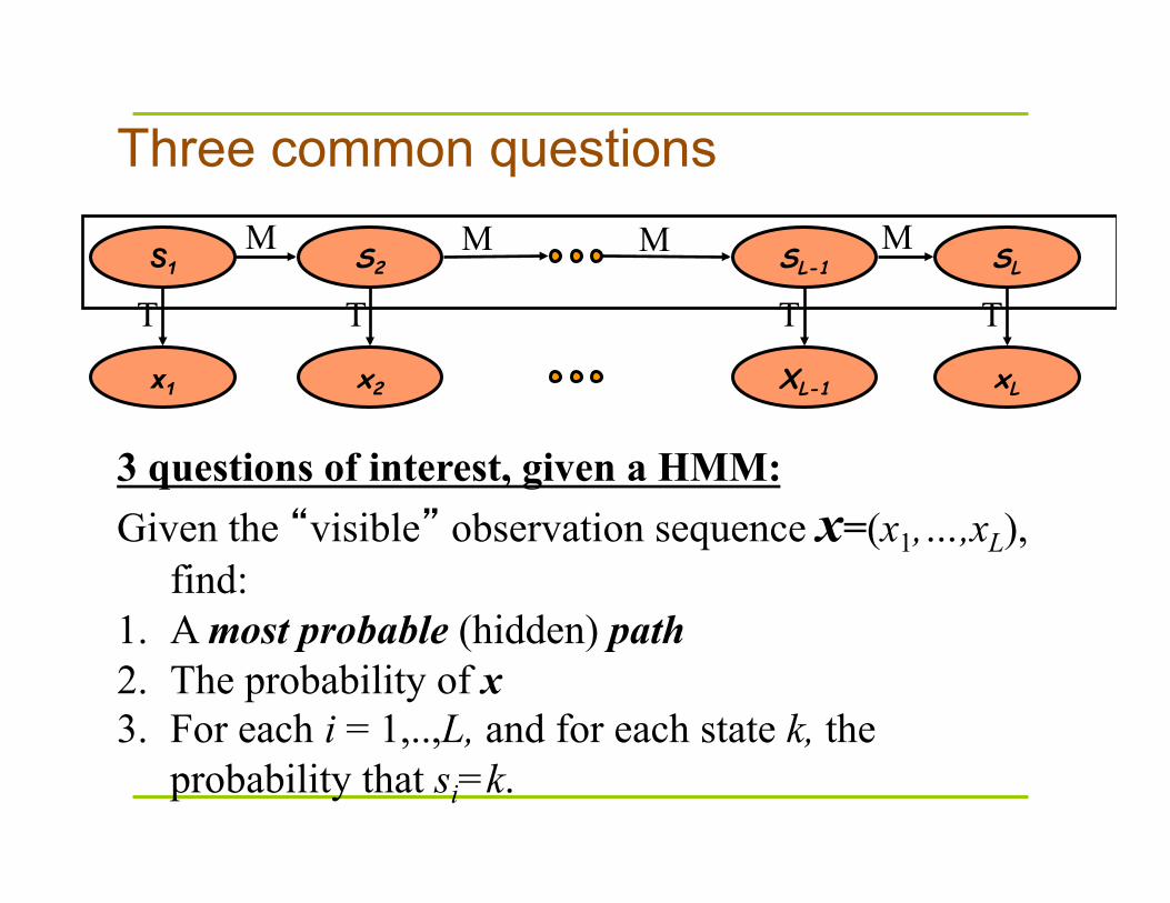
Three common questions

3 questions of interest, given a HMM: Given the “visible” observation sequence x=(x1,…,xL),

find: 1.  A most probable (hidden) path 2.  The probability of x 3.  For each i = 1,..,L, and for each state k, the

probability that si=k.

S1 S2 SL-1 SL

x1 x2 XL-1 xL

M M M M

T T T T

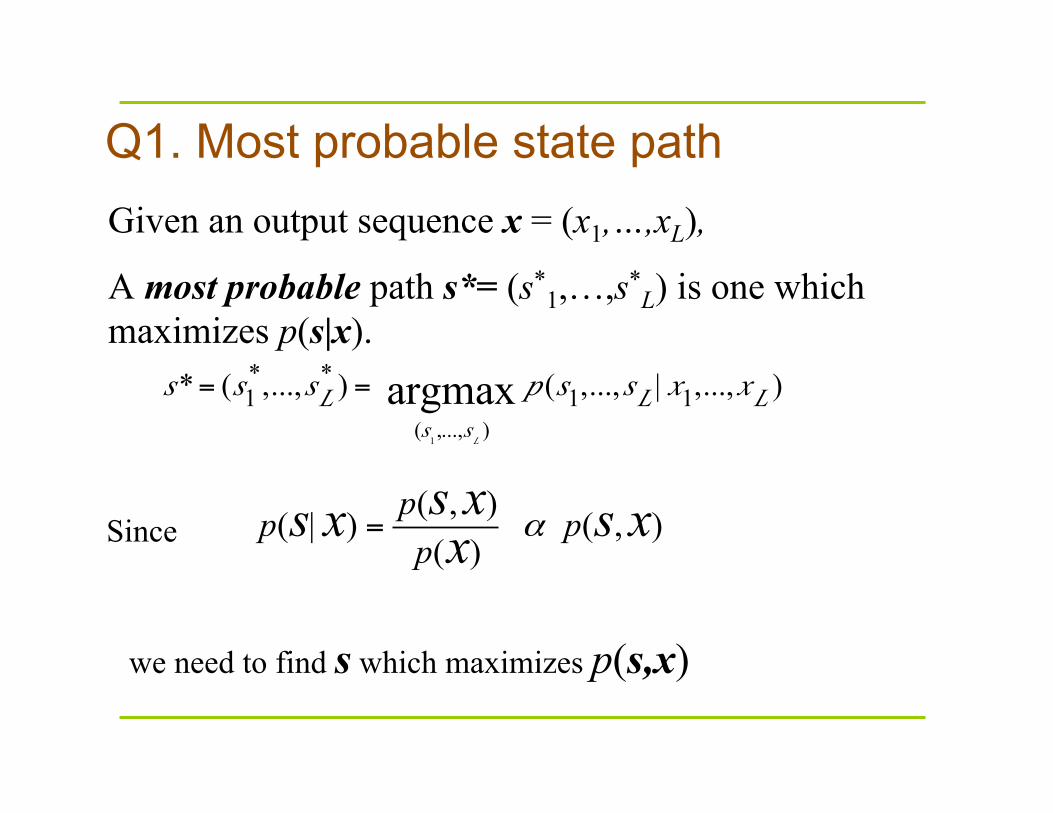
Q1. Most probable state path

s*= (s1*,...,sL

* ) = (s

1,...,s

L)

argmax p (s1,...,sL | x1,...,xL )

Given an output sequence x = (x1,…,xL),

A most probable path s*= (s*1,…,s*

L) is one which maximizes p(s|x).

( , ) ( | ) ( , )( )

pp pps xs x s xx α=Since

we need to find s which maximizes p(s,x)

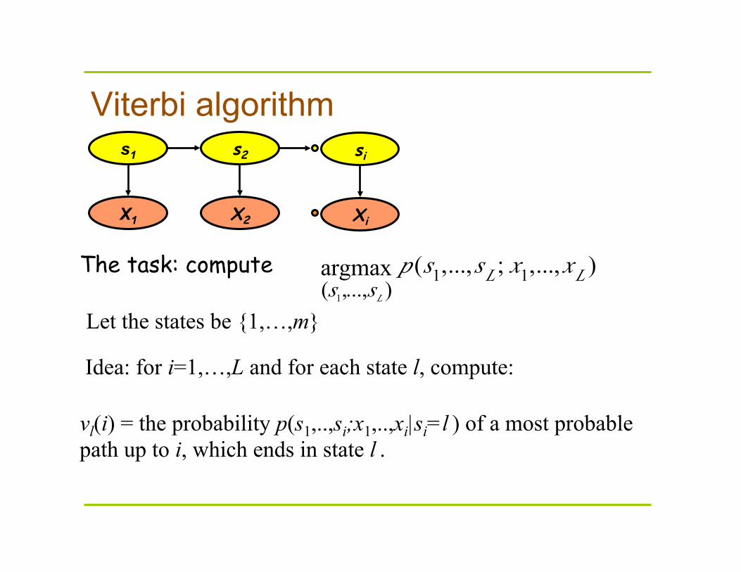
Viterbi algorithm

(s1,...,sL )argmax p (s1,...,sL ; x1,...,xL )

s1 s2

X1 X2

si

Xi

The task: compute

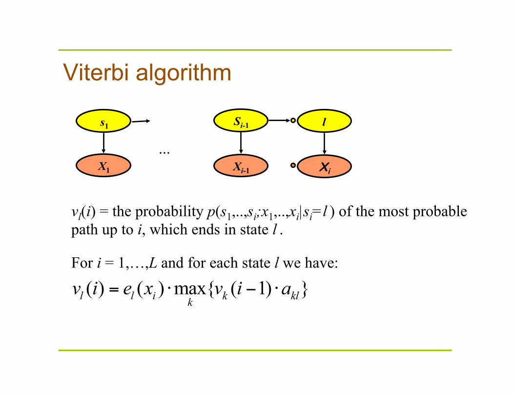
vl(i) = the probability p(s1,..,si;x1,..,xi|si=l ) of a most probable path up to i, which ends in state l .

Let the states be {1,…,m}

Idea: for i=1,…,L and for each state l, compute:

Viterbi algorithm

( ) ( ) max{ ( 1) }l l i k klkv i e x v i a= ⋅ − ⋅

vl(i) = the probability p(s1,..,si;x1,..,xi|si=l ) of the most probable path up to i, which ends in state l .

For i = 1,…,L and for each state l we have:

s1 Si-1

X1 Xi-1

l

Xi

...

Viterbi algorithm s1 s2 sL-1 sL

X1 X2 XL-1 XL

si

Xi

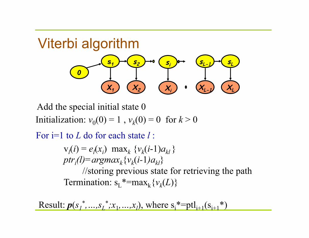
For i=1 to L do for each state l : vl(i) = el(xi) maxk {vk(i-1)akl } ptri(l)=argmaxk{vk(i-1)akl} //storing previous state for retrieving the path Termination: sL*=maxk{vk(L)}

Initialization: v0(0) = 1 , vk(0) = 0 for k > 0

0

Add the special initial state 0

Result: p(s1*,…,sL

*;x1,…,xl), where si*=ptli+1(si+1*)

Example: a fair casino problem

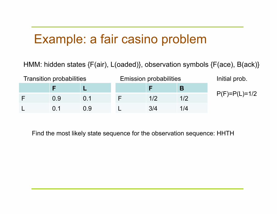
F L F 0.9 0.1 L 0.1 0.9

Transition probabilities

HMM: hidden states {F(air), L(oaded)}, observation symbols {F(ace), B(ack)}

F B F 1/2 1/2 L 3/4 1/4

Emission probabilities Initial prob. P(F)=P(L)=1/2

Find the most likely state sequence for the observation sequence: HHTH

Q2. Computing p(x)

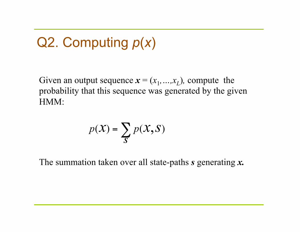
( ) ( ),p px x s=∑S

Given an output sequence x = (x1,…,xL), compute the probability that this sequence was generated by the given HMM:

The summation taken over all state-paths s generating x.

Forward algorithm

( ) ( ) ( 1)l l i k klk

F i e x F i a= ⋅ − ⋅∑

? ?

X1 Xi-1

si

Xi

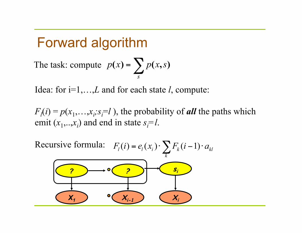
The task: compute

Idea: for i=1,…,L and for each state l, compute: Fl(i) = p(x1,…,xi;si=l ), the probability of all the paths which emit (x1,..,xi) and end in state si=l.

Recursive formula:

∑=s

sxpxp ),()(

Forward algorithm s1 s2 sL-1 sL

X1 X2 XL-1 XL

si

Xi

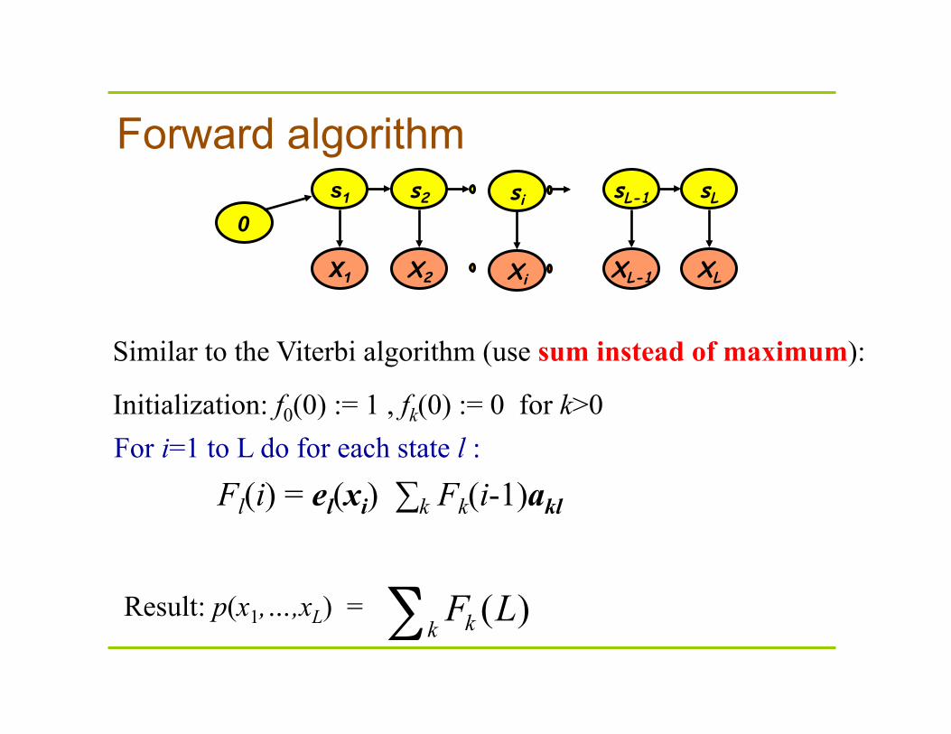
For i=1 to L do for each state l :

Fl(i) = el(xi) ∑k Fk(i-1)akl

Initialization: f0(0) := 1 , fk(0) := 0 for k>0

0

Similar to the Viterbi algorithm (use sum instead of maximum):

Result: p(x1,…,xL) = ( )kkF L∑

Given an output sequence x = (x1,…,xL),

Compute for each i=1,…,l and for each state k the probability that si = k.

This helps to reply queries like: what is the probability that si is in a CpG island, etc.

Q3. Distribution of Si, given x

Solution in two stages

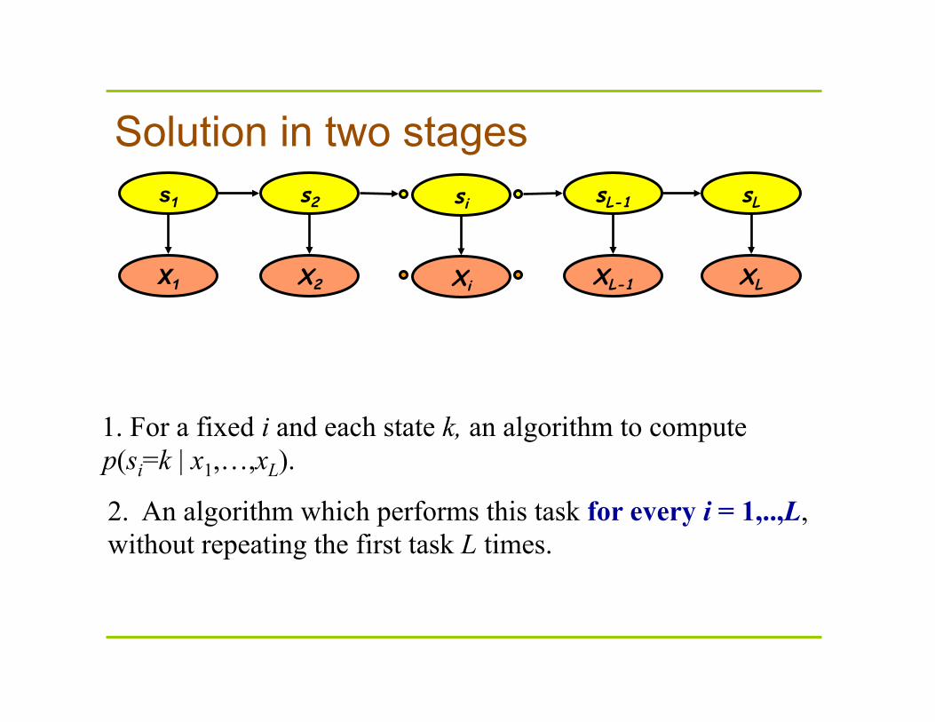
1.  For a fixed i and each state k, an algorithm to compute p(si=k | x1,…,xL).

s1 s2 sL-1 sL

X1 X2 XL-1 XL

si

Xi

2. An algorithm which performs this task for every i = 1,..,L, without repeating the first task L times.

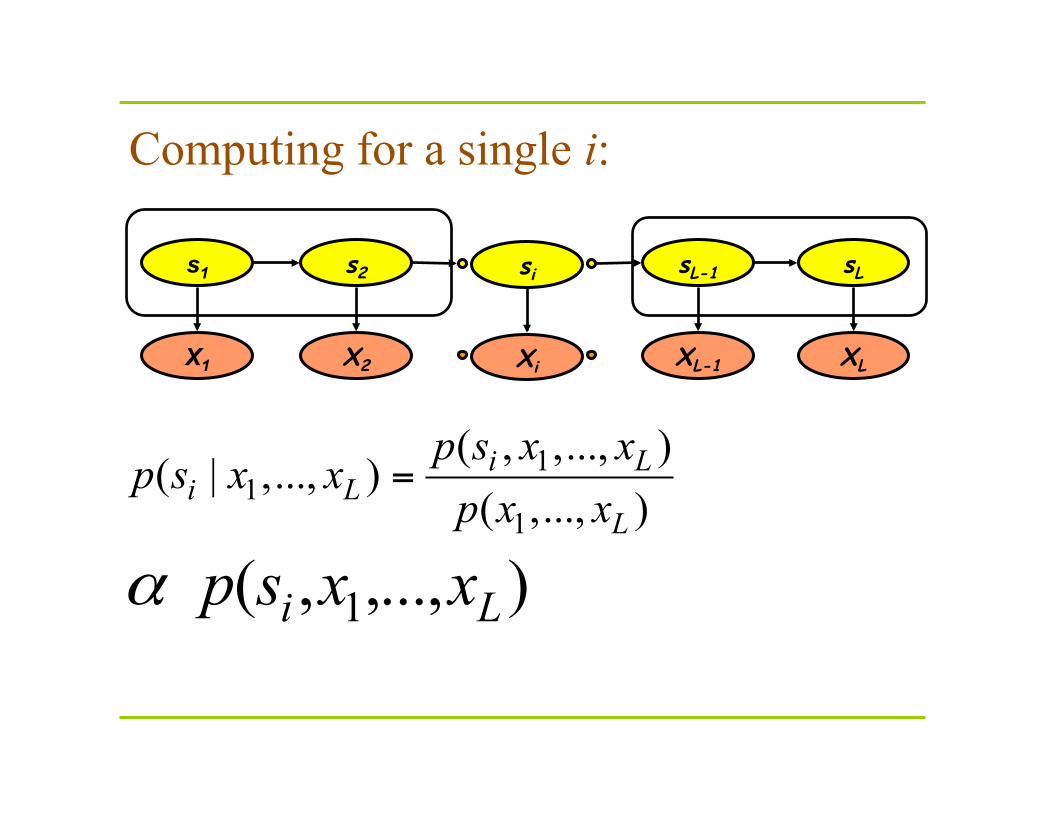
Computing for a single i:

11

1

( , ,..., )( | ,..., )

( ,..., )

1 ( , ,..., )

i Li L

L

p s x xp s x x

p x x

i Lp s x xα

=

s1 s2 sL-1 sL

X1 X2 XL-1 XL

si

Xi

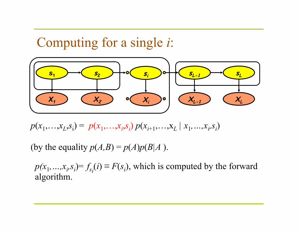
p(x1,…,xL,si) = p(x1,…,xi,si) p(xi+1,…,xL | x1,…,xi,si) (by the equality p(A,B) = p(A)p(B|A ).

s1 s2 sL-1 sL

X1 X2 XL-1 XL

si

Xi

p(x1,…,xi,si)= fsi(i) ≡ F(si), which is computed by the forward algorithm.

Computing for a single i:

F(si): The forward algorithm: s1 s2 sL-1 sL

X1 X2 XL-1 XL

si

Xi

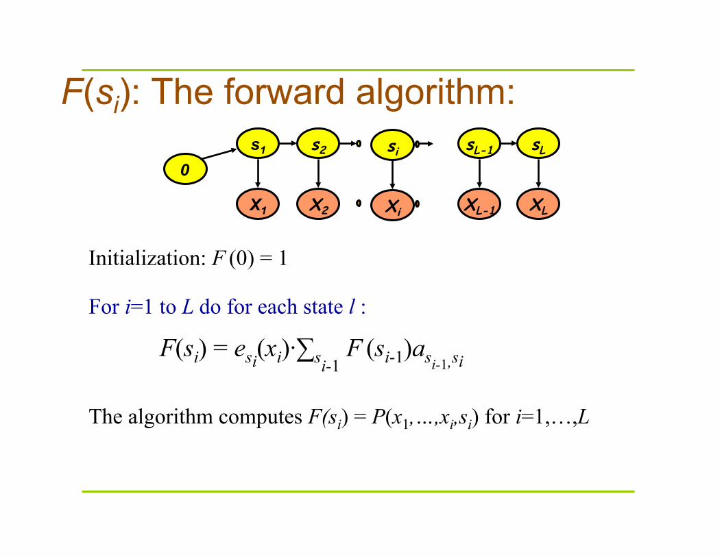
For i=1 to L do for each state l :

F(si) = esi(xi)·∑si-1 F (si-1)asi-1,si

Initialization: F (0) = 1

0

The algorithm computes F(si) = P(x1,…,xi,si) for i=1,…,L

B(si): The backward algorithm

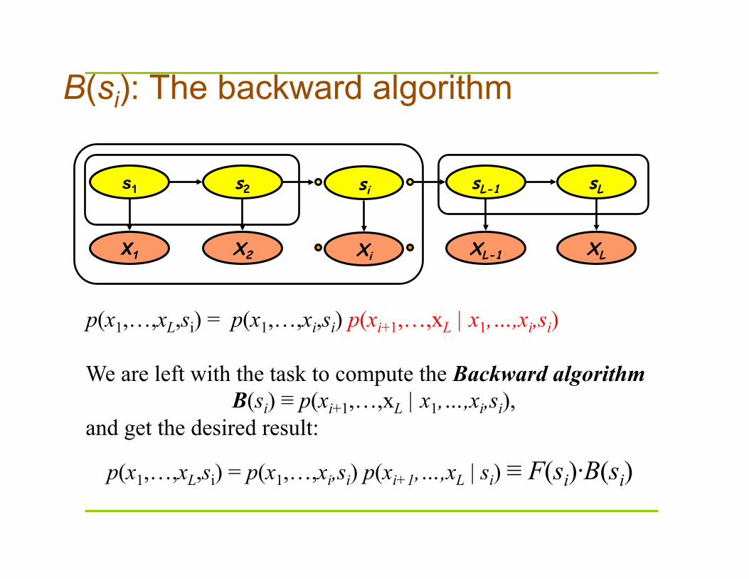
p(x1,…,xL,si) = p(x1,…,xi,si) p(xi+1,…,xL | x1,…,xi,si)

s1 s2 sL-1 sL

X1 X2 XL-1 XL

si

Xi

We are left with the task to compute the Backward algorithm B(si) ≡ p(xi+1,…,xL | x1,…,xi,si),

and get the desired result:

p(x1,…,xL,si) = p(x1,…,xi,si) p(xi+1,…,xL | si) ≡ F(si)·B(si)

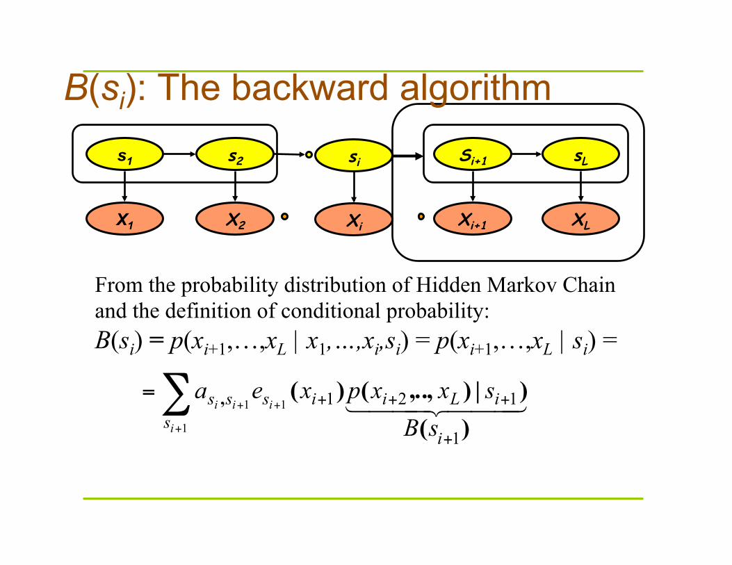
B(si): The backward algorithm s1 s2 Si+1 sL

X1 X2 Xi+1 XL

si

Xi

From the probability distribution of Hidden Markov Chain and the definition of conditional probability: B(si) = p(xi+1,…,xL | x1,…,xi,si) = p(xi+1,…,xL | si) =

∑+

++

+

+++=1

11

1

121 i

iiis

i

iLiisss

sBsxxpxea

)()|),..,()(,

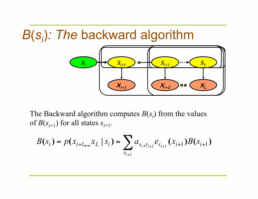
B(si): The backward algorithm

Si+2 SL

Xi+2 XL

Si Si+1

Xi+1

∑+

++ +++ ==1

11 111i

iiis

iisssiLii sBxeasxxpsB )()()|()( ,,..,

The Backward algorithm computes B(si) from the values of B(si+1) for all states si+1.

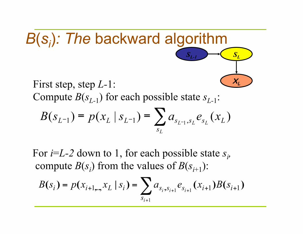
B(si): The backward algorithm SL-1 SL

XL First step, step L-1: Compute B(sL-1) for each possible state sL-1:

For i=L-2 down to 1, for each possible state si, compute B(si) from the values of B(si+1):

∑+

++ +++ ==1

11 111i

iiis

iisssiLii sBxeasxxpsB )()()|()( ,,..,

∑ - = = - -

L L L L

s L s s s L L L x e a s x p s B ) ( ) | ( ) ( , 1 1 1

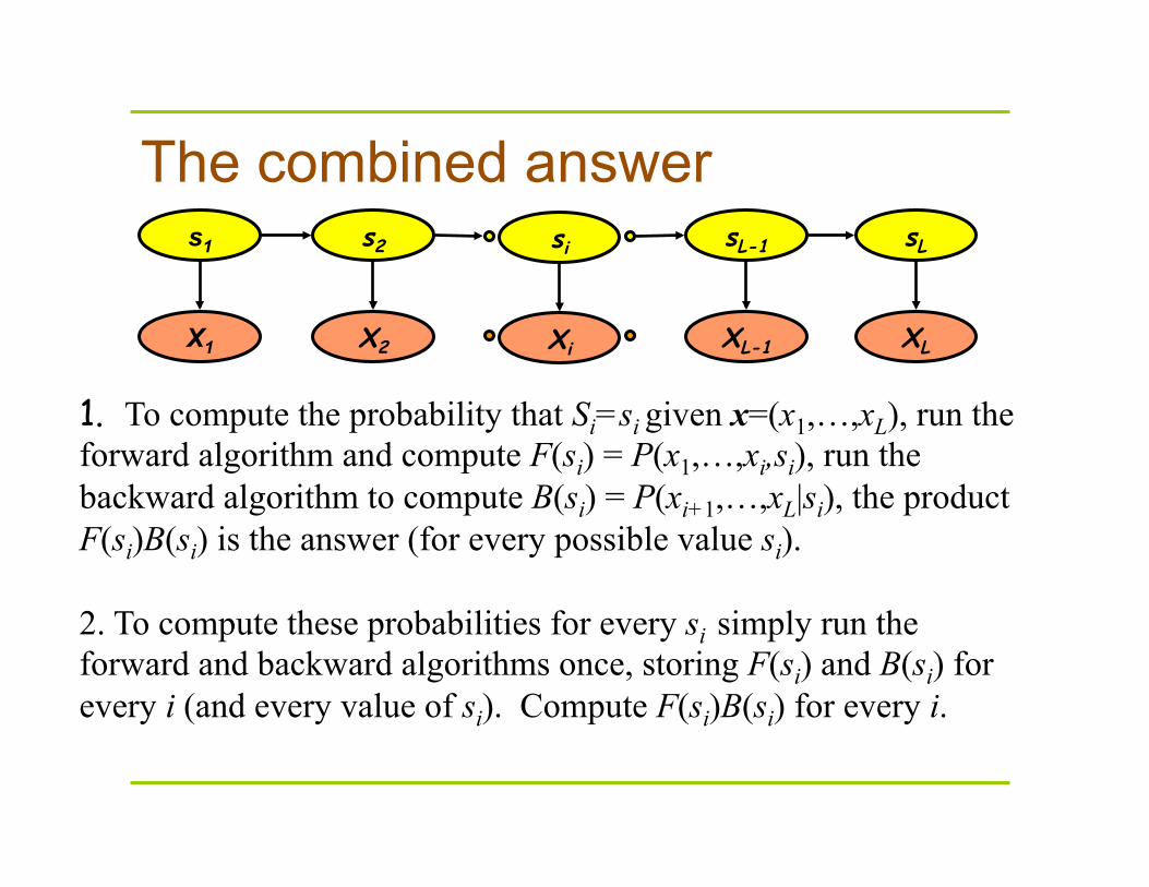
The combined answer

1. To compute the probability that Si=si given x=(x1,…,xL), run the forward algorithm and compute F(si) = P(x1,…,xi,si), run the backward algorithm to compute B(si) = P(xi+1,…,xL|si), the product F(si)B(si) is the answer (for every possible value si). 2. To compute these probabilities for every si simply run the forward and backward algorithms once, storing F(si) and B(si) for every i (and every value of si). Compute F(si)B(si) for every i.

s1 s2 sL-1 sL

X1 X2 XL-1 XL

si

Xi

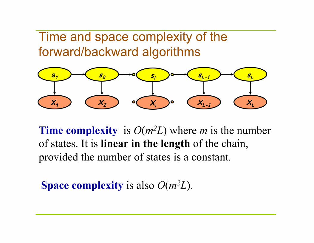
Time and space complexity of the forward/backward algorithms

Time complexity is O(m2L) where m is the number of states. It is linear in the length of the chain, provided the number of states is a constant.

s1 s2 sL-1 sL

X1 X2 XL-1 XL

si

Xi

Space complexity is also O(m2L).

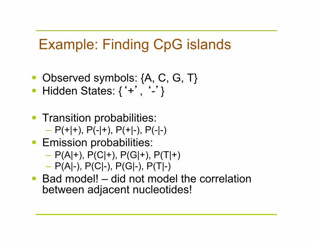
Example: Finding CpG islands

  Observed symbols: {A, C, G, T}   Hidden States: {‘+’, ‘-’}

  Transition probabilities: –  P(+|+), P(-|+), P(+|-), P(-|-)

  Emission probabilities: –  P(A|+), P(C|+), P(G|+), P(T|+) –  P(A|-), P(C|-), P(G|-), P(T|-)

  Bad model! – did not model the correlation between adjacent nucleotides!

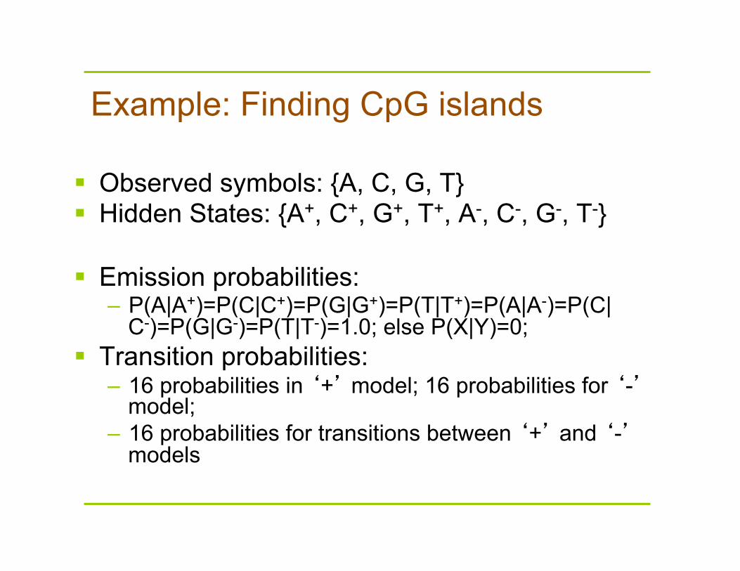
Example: Finding CpG islands

  Observed symbols: {A, C, G, T}   Hidden States: {A+, C+, G+, T+, A-, C-, G-, T-}

  Emission probabilities: –  P(A|A+)=P(C|C+)=P(G|G+)=P(T|T+)=P(A|A-)=P(C|

C-)=P(G|G-)=P(T|T-)=1.0; else P(X|Y)=0;   Transition probabilities:

–  16 probabilities in ‘+’ model; 16 probabilities for ‘-’ model;

–  16 probabilities for transitions between ‘+’ and ‘-’ models

Example: Eukaryotic gene finding

  In eukaryotes, the gene is a combination of coding segments (exons) that are interrupted by non-coding segments (introns)

  This makes computational gene prediction in eukaryotes even more difficult

  Prokaryotes don’t have introns - Genes in prokaryotes are continuous

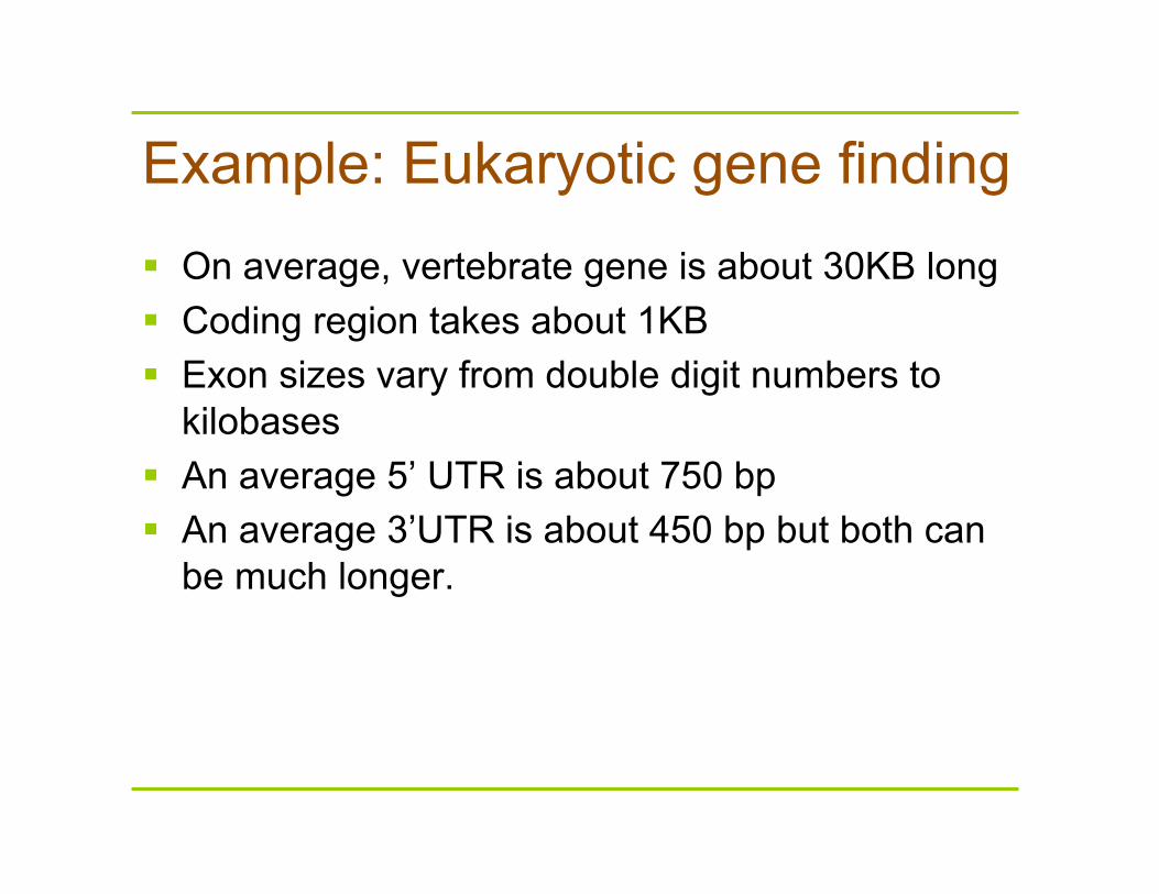
Example: Eukaryotic gene finding   On average, vertebrate gene is about 30KB long   Coding region takes about 1KB   Exon sizes vary from double digit numbers to

kilobases   An average 5’ UTR is about 750 bp   An average 3’UTR is about 450 bp but both can

be much longer.

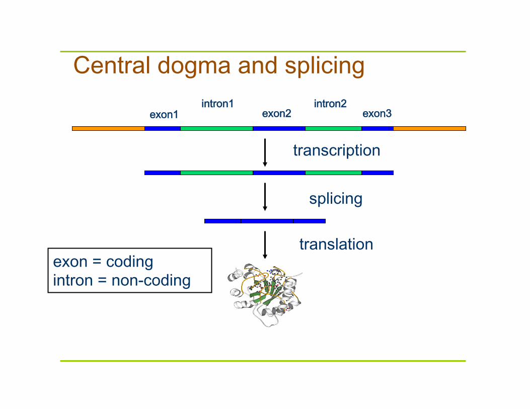
Central dogma and splicing

exon1 exon2 exon3 intron1 intron2

transcription

translation

splicing

exon = coding intron = non-coding

Splicing signals

  Try to recognize location of splicing signals at exon-intron junctions –  This has yielded a weakly conserved donor splice

site and acceptor splice site   Profiles for sites are still weak, and lends the

problem to the Hidden Markov Model (HMM) approaches, which capture the statistical dependencies between sites

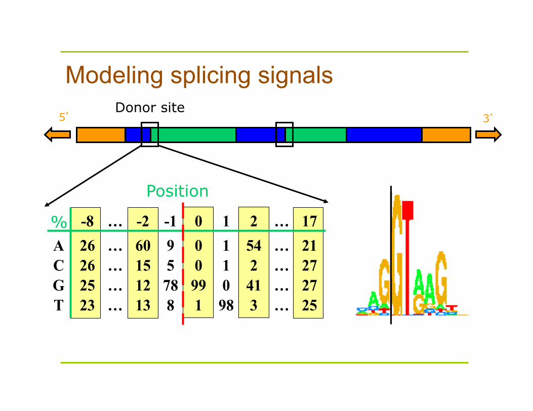
5’ 3’ Donor site

Position

% -8 … -2 -1 0 1 2 … 17A 26 … 60 9 0 1 54 … 21C 26 … 15 5 0 1 2 … 27G 25 … 12 78 99 0 41 … 27T 23 … 13 8 1 98 3 … 25

Modeling splicing signals

Genscan model

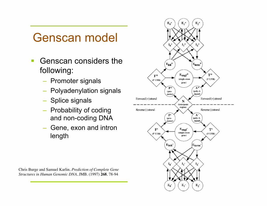
  Genscan considers the following: –  Promoter signals –  Polyadenylation signals –  Splice signals –  Probability of coding

and non-coding DNA –  Gene, exon and intron

length

Chris Burge and Samuel Karlin, Prediction of Complete Gene Structures in Human Genomic DNA, JMB. (1997) 268, 78-94

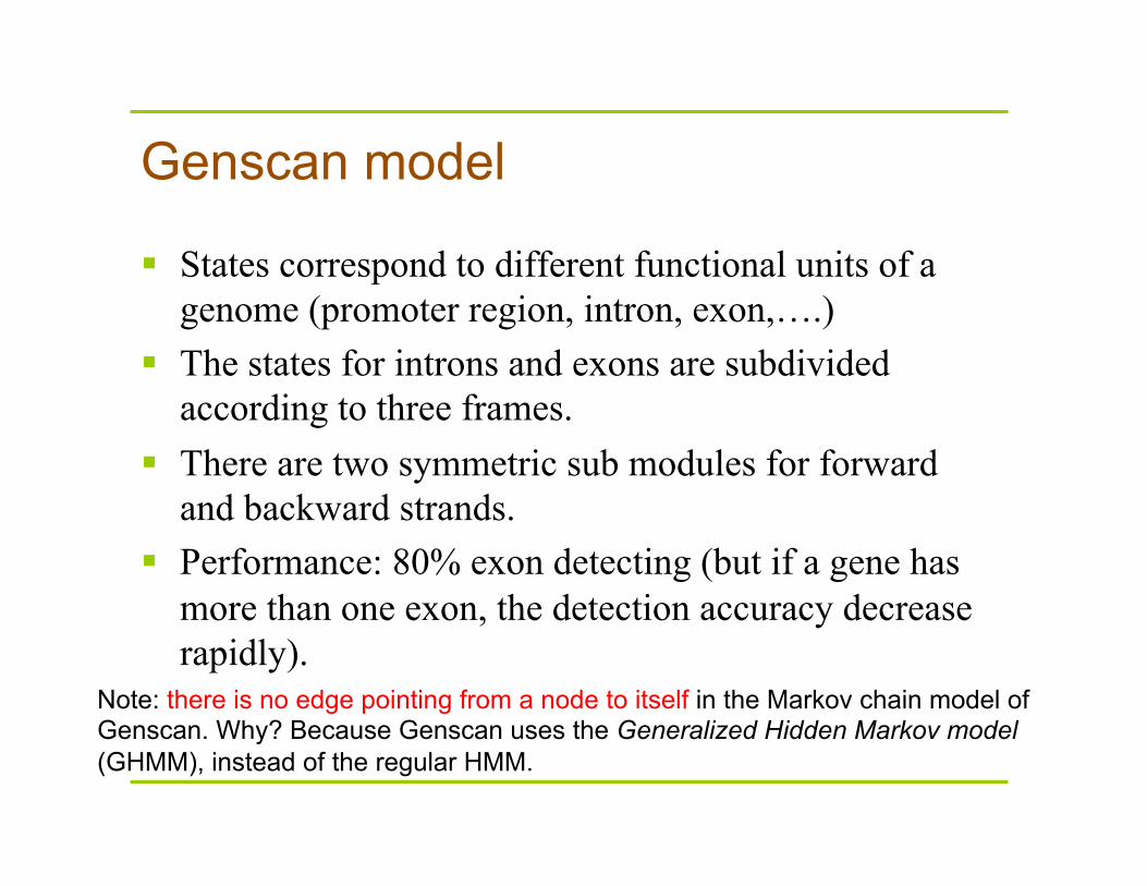
Note: there is no edge pointing from a node to itself in the Markov chain model of Genscan. Why? Because Genscan uses the Generalized Hidden Markov model (GHMM), instead of the regular HMM.

Genscan model

  States correspond to different functional units of a genome (promoter region, intron, exon,….)

  The states for introns and exons are subdivided according to three frames.

  There are two symmetric sub modules for forward and backward strands.

  Performance: 80% exon detecting (but if a gene has more than one exon, the detection accuracy decrease rapidly).

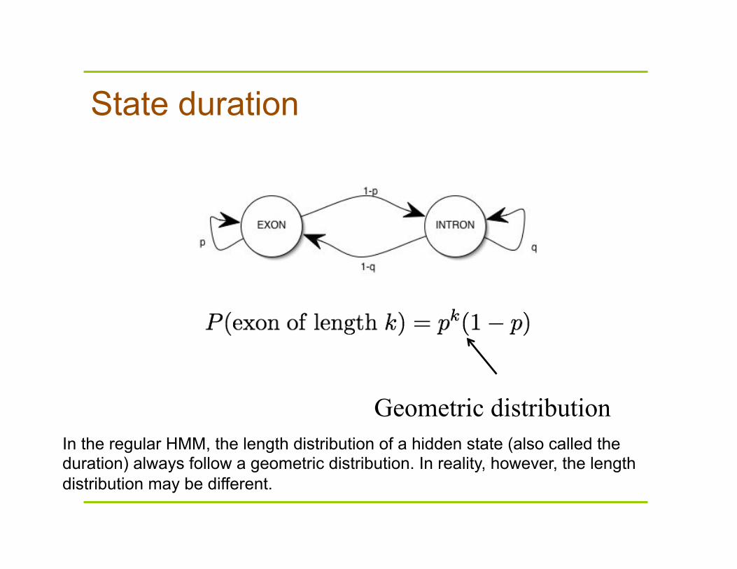
State duration

Geometric distribution In the regular HMM, the length distribution of a hidden state (also called the duration) always follow a geometric distribution. In reality, however, the length distribution may be different.

Generalized HMMs (Hidden semi-Markov models)

 Based on a variant-length Markov chain;  The (emitted) output of a state is a string of finite

length;  For a given state, the output string and its length are

according to a probability distribution;  Different states may have different length

distributions.

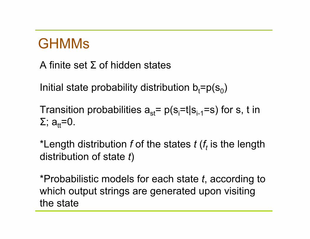
GHMMs A finite set Σ of hidden states

Initial state probability distribution bt=p(s0)

Transition probabilities ast= p(si=t|si-1=s) for s, t in Σ; att=0.

*Length distribution f of the states t (ft is the length distribution of state t)

*Probabilistic models for each state t, according to which output strings are generated upon visiting the state

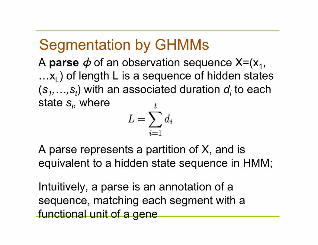
Segmentation by GHMMs A parse ϕ of an observation sequence X=(x1,…xL) of length L is a sequence of hidden states (s1,…,st) with an associated duration di to each state si, where

A parse represents a partition of X, and is equivalent to a hidden state sequence in HMM;

Intuitively, a parse is an annotation of a sequence, matching each segment with a functional unit of a gene

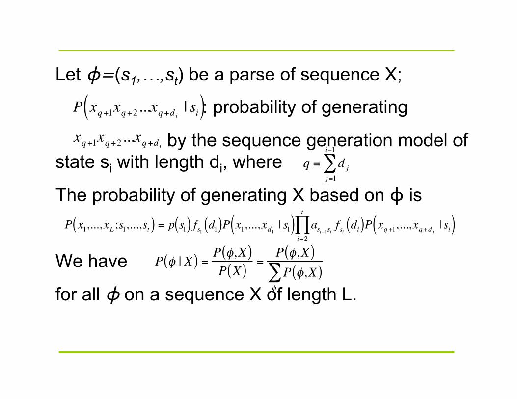
Let ϕ=(s1,…,st) be a parse of sequence X;

: probability of generating

by the sequence generation model of state si with length di, where

The probability of generating X based on ϕ is

We have

for all ϕ on a sequence X of length L.

€

P xq+1xq+2...xq+d i| si( )

€

xq+1xq+2...xq+d i

€

q = d jj=1

i−1

∑

€

P x1,...,xL ;s1,...,st( ) = p s1( ) fs1 d1( )P x1,...,xd1 | s1( ) asi−1si fsi di( )P xq+1,...,xq+d i| si( )

i=2

t

∏

€

P φ | X( ) =P φ,X( )P X( )

=P φ,X( )P φ,X( )

φ

∑

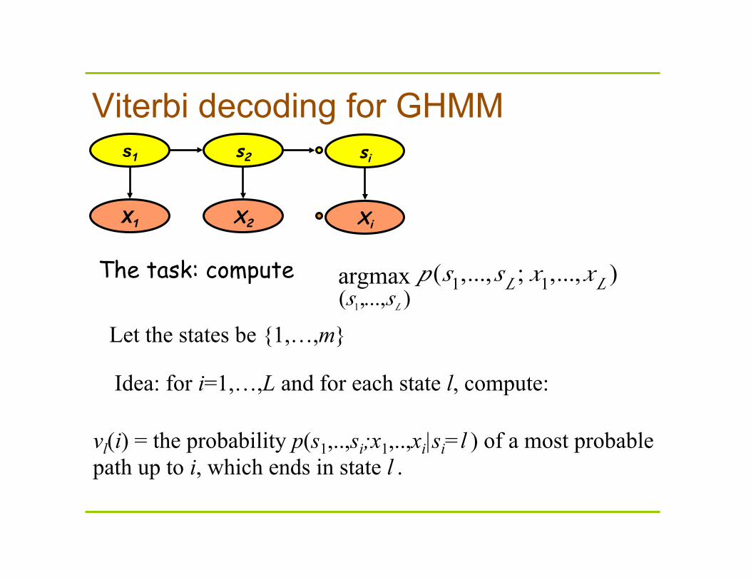
Viterbi decoding for GHMM

(s1,...,sL )argmax p (s1,...,sL ; x1,...,xL )

s1 s2

X1 X2

si

Xi

The task: compute

vl(i) = the probability p(s1,..,si;x1,..,xi|si=l ) of a most probable path up to i, which ends in state l .

Let the states be {1,…,m}

Idea: for i=1,…,L and for each state l, compute:

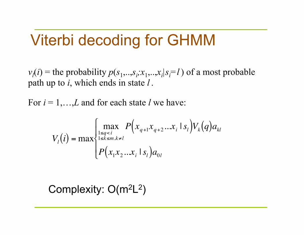
Viterbi decoding for GHMM

€

Vl i( ) =maxmax

1≤q< i1≤k≤m,k≠ l

P xq+1xq+2...xi | sl( )Vk q( )akl

P x1x2 ...xi | sl( )a0l

$

% &

' &

vl(i) = the probability p(s1,..,si;x1,..,xi|si=l ) of a most probable path up to i, which ends in state l .

For i = 1,…,L and for each state l we have:

Complexity: O(m2L2)

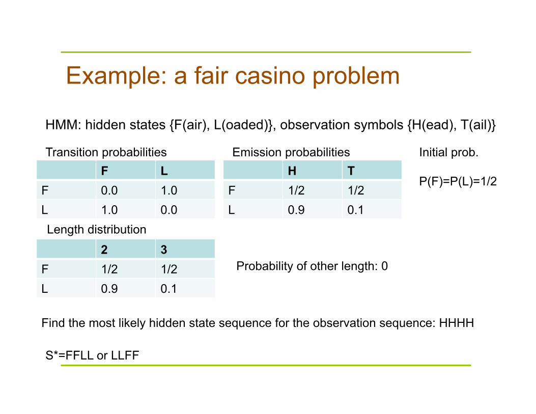
Example: a fair casino problem

F L F 0.0 1.0 L 1.0 0.0

Transition probabilities

HMM: hidden states {F(air), L(oaded)}, observation symbols {H(ead), T(ail)}

H T F 1/2 1/2 L 0.9 0.1

Emission probabilities Initial prob. P(F)=P(L)=1/2

Find the most likely hidden state sequence for the observation sequence: HHHH

S*=FFLL or LLFF

2 3 F 1/2 1/2 L 0.9 0.1

Length distribution

Probability of other length: 0