Lecture 7: Markov Chain Monte Carlo

Lecture 7: Markov Chain Monte Carlo

4F13: Machine Learning

Zoubin Ghahramani and Carl Edward Rasmussen

Department of Engineering, University of Cambridge

February 8th and 13th, 2008

Ghahramani & Rasmussen (CUED) Lecture 7: Markov Chain Monte Carlo February 8th and 13th, 2008 1 / 28

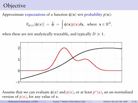
Objective

Approximate expectations of a function φ(x) wrt probability p(x):

Ep(x)[φ(x)] = φ =

∫φ(x)p(x)dx, where x ∈ RD

,

when these are not analytically tractable, and typically D� 1.

−1

0

1

2

Assume that we can evaluate φ(x) and p(x), or at least p∗(x), an un-normalizedversion of p(x), for any value of x.


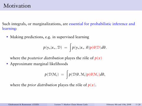
Motivation

Such integrals, or marginalizations, are essential for probabilistic inference andlearning:

• Making predictions, e.g. in supervised learning

p(y∗|x∗,D) =

∫p(y∗|x∗, θ)p(θ|D)dθ,

where the posterior distribution playes the rôle of p(x)

• Approximate marginal likelihoods

p(D|Mi) =

∫p(D|θ,Mi)p(θ|Mi)dθ,

where the prior distribution playes the rôle of p(x).


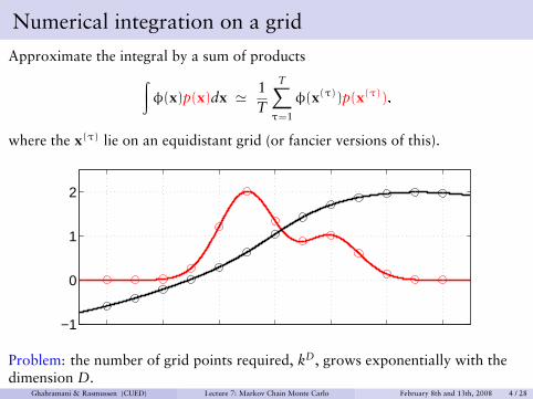
Numerical integration on a grid

Approximate the integral by a sum of products∫φ(x)p(x)dx ' 1

T

T∑τ=1

φ(x(τ))p(x(τ)),

where the x(τ) lie on an equidistant grid (or fancier versions of this).

−1

0

1

2

Problem: the number of grid points required, kD, grows exponentially with thedimension D.


Monte Carlo

The foundation identity for Monte Carlo approximations is

E[φ(x)] ' �φ =1T

T∑τ=1

φ(x(τ)). where x(τ) ∼ p(x).

Under mild conditions, �φ→ E[φ(x)] as T →∞.

For moderate T, �φ may still be a good approximation. In fact it is an unbiasedestimate with

V[�φ] =V[φ]

T, where V[φ] =

∫ (φ(x) − φ

)2p(x)dx.

Note, that this variance in independent of the dimension D of x.

This is great, but how do we generate random samples from p(x)?


Random number generation

There are (pseudo-) random number generators for the uniform [0; 1] distribution.

Transformation methods exist to turn these into other simple univariatedistributions, such as Gaussian, Gamma, . . . , as well as some multivariatedistributions e.g. Gaussian and Dirichlet.

Example: p(x) is uniform [0; 1]. The transformation y = − log(x) yields:

p(y) = p(x)∣∣dxdy

∣∣ = exp(−y),

i.e. an exponential distribution.

Typically p(x) may be more complicated.

How can we generate samples from a (multivariate) distribution p(x)?

Idea: we can discretize p(x), and sample from the discrete multinomialdistribution. Will this work?


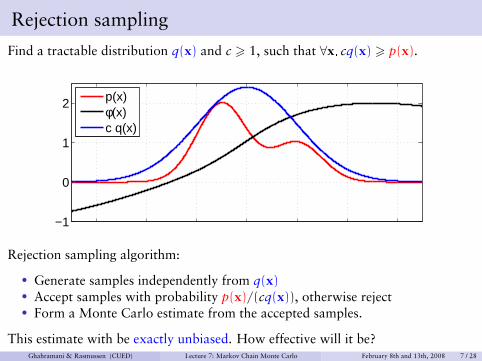
Rejection sampling

Find a tractable distribution q(x) and c > 1, such that ∀x, cq(x) > p(x).

−1

0

1

2

p(x)φ(x)c q(x)

Rejection sampling algorithm:

• Generate samples independently from q(x)• Accept samples with probability p(x)/(cq(x)), otherwise reject• Form a Monte Carlo estimate from the accepted samples.

This estimate with be exactly unbiased. How effective will it be?Ghahramani & Rasmussen (CUED) Lecture 7: Markov Chain Monte Carlo February 8th and 13th, 2008 7 / 28

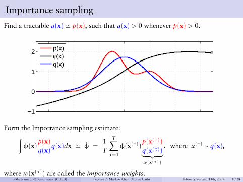
Importance sampling

Find a tractable q(x) ' p(x), such that q(x) > 0 whenever p(x) > 0.

−1

0

1

2

p(x)φ(x)q(x)

Form the Importance sampling estimate:∫φ(x)

p(x)

q(x)q(x)dx ' �φ =

1T

T∑τ=1

φ(x(τ))p(x(τ))

q(x(τ))︸︷︷︸w(x(τ))

, where x(τ) ∼ q(x),

where w(x(τ)) are called the importance weights.Ghahramani & Rasmussen (CUED) Lecture 7: Markov Chain Monte Carlo February 8th and 13th, 2008 8 / 28

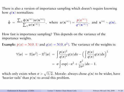
There is also a version of importance sampling which doesn’t require knowinghow q(x) normalizes:

�φ =

∑τ φ(x(τ))w(x(τ))∑

τ w(x(τ)), where w(x(τ)) =

p(x(τ))

q∗(x(τ)), and x(τ) ∼ q(x).

How fast is importance sampling? This depends on the variance of theimportance weights.

Example: p(x) = N(0, 1) and q(x) = N(0,σ2). The variance of the weights is:

V[w] = E[w2] − E2[w] =

∫p(x)2

q(x)2 q(x)dx −( ∫

p(x)

q(x)q(x)dx

)2

= σ

∫exp(−x2 +

x2

2σ2 )dx − 1.

which only exists when σ >√

1/2. Morale: always chose q(x) to be wider, have‘heavier tails’ than p(x) to avoid this problem.


Rejection and Importance sampling

In the multivariate case with Gaussian q(x) we must be able to guarantee that nodirection exist when we underestimate the width by more than a factor of

√2.

In fact, both rejection and importance sampling have severe problems in highdimensions, since it is virtually impossible to get q(x) close enough to p(x), seeMacKay chapter 29 for details.


Independent Sampling vs. Markov Chains

So far, we’ve considered two methods, Rejection and Importance Sampling,which were both based on independent samples from q(x).

However, for many problems of practical interest it is difficult or impossible tofind q(x) with the necessary properties.

Instead we can abandon the idea of independent sampling, and instead rely on aMarkov Chain to generate dependent samples from the target distribution.

Independence would be a nice thing, but it is not necessary for the Monte Carloestimate to be valid.


Markov Chain Monte Carlo

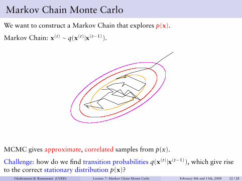
We want to construct a Markov Chain that explores p(x).

Markov Chain: x(t) ∼ q(x(t)|x(t−1)).

MCMC gives approximate, correlated samples from p(x).

Challenge: how do we find transition probabilities q(x(t)|x(t−1)), which give riseto the correct stationary distribution p(x)?


Discrete Markov Chains

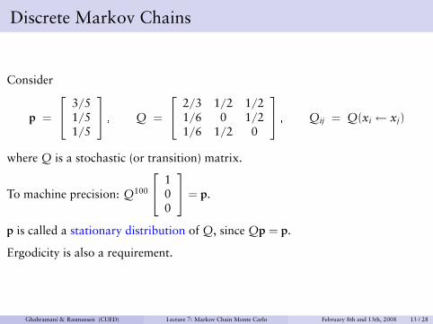
Consider

p =

3/51/51/5

, Q =

2/3 1/2 1/21/6 0 1/21/6 1/2 0

, Qij = Q(xi ← xj)

where Q is a stochastic (or transition) matrix.

To machine precision: Q100

100

= p.

p is called a stationary distribution of Q, since Qp = p.

Ergodicity is also a requirement.


In Continuous Spaces

In continuous spaces transitions are governed by q(x ′|x).

Now, p(x) is a stationary distribution for q(x ′|x) if∫q(x ′|x)p(x)dx = p(x ′).


Detailed Balance

Detailed balance means

q(x ′|x)p(x) = q(x|x ′)p(x ′).

Now, integrating both sides wrt x, we get∫q(x ′|x)p(x)dx =

∫q(x|x ′)p(x ′)dx = p(x ′).

Thus, detailed balance implies the existence of a stationary distribution


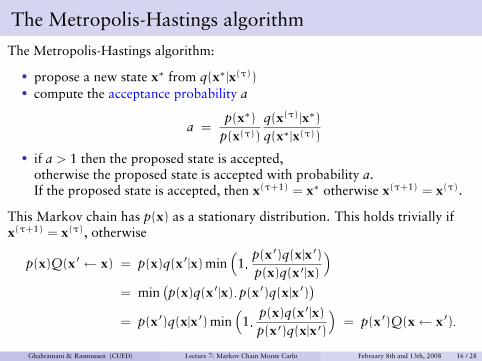
The Metropolis-Hastings algorithm

The Metropolis-Hastings algorithm:

• propose a new state x∗ from q(x∗|x(τ))

• compute the acceptance probability a

a =p(x∗)

p(x(τ))

q(x(τ)|x∗)

q(x∗|x(τ))

• if a > 1 then the proposed state is accepted,otherwise the proposed state is accepted with probability a.If the proposed state is accepted, then x(τ+1) = x∗ otherwise x(τ+1) = x(τ).

This Markov chain has p(x) as a stationary distribution. This holds trivially ifx(τ+1) = x(τ), otherwise

p(x)Q(x ′ ← x) = p(x)q(x ′|x) min(

1,p(x ′)q(x|x ′)

p(x)q(x ′|x)

)= min

(p(x)q(x ′|x), p(x ′)q(x|x ′)

)= p(x ′)q(x|x ′) min

(1,

p(x)q(x ′|x)

p(x ′)q(x|x ′)

)= p(x ′)Q(x← x ′).


Some properties of Metropolis Hastings

• The Metropolis algorithm has p(x) as its stationary distribution• If q(x∗|x(τ)) is symmetric, then

• the expression for a simplifies to a = p(x∗)/p(x(τ))• the algorithm then always accepts if the proposed state has higher

probability than the current state and sometimes accepts a state withlower probability.

• we only need the ratio of p(x)’s, so we don’t need the normalization constant.This is important, e.g. when sampling from a posterior distribution.

The Metropolis algorithm can be widely applied, you just need to specify aproposal distribution.

The proposal distribution must satisfy some (mild) constraints (related toergodicity).


The Proposal Distribution

Often, Gaussian proposal distributions are used, centered on the current state.You need to specify the width of the proposal distribution.

What happens if the proposal distribution is

• too wide?• too narrow?


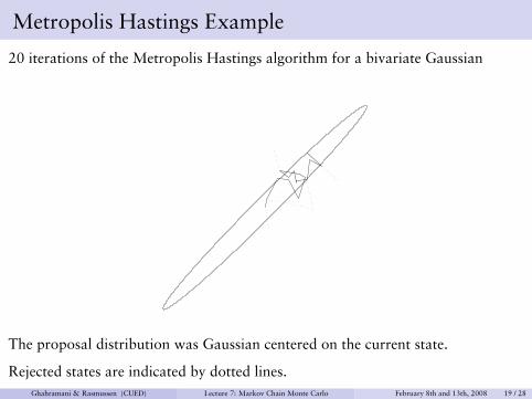
Metropolis Hastings Example

20 iterations of the Metropolis Hastings algorithm for a bivariate Gaussian

The proposal distribution was Gaussian centered on the current state.

Rejected states are indicated by dotted lines.Ghahramani & Rasmussen (CUED) Lecture 7: Markov Chain Monte Carlo February 8th and 13th, 2008 19 / 28

Random walks

When exploring a distribution with the Metropolis algorithm, the proposal has tobe narrow to avoid too many rejections.

If a typical step moves a distance ε, then one needs an expected T = (L/ε)2 stepsto travel a distance of L. This is a problem with random walk behavior.

Notice that strong correlations can slow down the Metropolis algorithm, becausethe proposal width should be set according to the tightest direction.


Variants of the Metropolis algorithm

Instead of proposing a new state by changing simultaneously all components ofthe state, you can concatenate different proposals changing one component at atime.

For example, qj(x ′|x), such that x ′i = xi, ∀i 6= j.

Now, cycle through the qj(x ′|x) in turn.

This is valid as

• each iteration obeys detailed balance• the sequence guarantees ergodicity


Gibbs sampling

Updating one coordinate at a time, and choosing the proposal distribution to bethe conditional distribution of that variable given all other variablesq(x ′

i |x) = p(x ′i |x6=i) we get

a = min(

1,p(x 6=i)p(x ′

i |x 6=i)p(xi|x ′6=i)

p(x6=i)p(xi|x6=i)p(x ′i |x 6=i)

)= 1,

i.e., we get an algorithm which always accepts. This is called the Gibbs samplingalgorithm.

If you can compute (and sample from) the conditionals, you can apply Gibbssampling.

This algorithm is completely parameter free.

Can also be applied to subsets of variables.


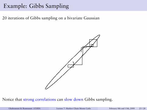
Example: Gibbs Sampling

20 iterations of Gibbs sampling on a bivariate Gaussian

Notice that strong correlations can slow down Gibbs sampling.


Hybrid Monte Carlo

Define a joint distribution over position and velocity

• p(x, v) = p(v)p(x) = e−E(x)−K(v) = e−H(x,v).• v independent of x and v ∼ N(0, 1).• sample in the joint space, then ignore the velocities to get the positions.

Markov chain:

• Gibbs sample velocities using N(0, 1)

• Simulate Hamiltonian dynamics through fictitious time, then negate velocity• ’proposal’ is deterministic and reversible• conservation of energy guarantees p(x, v) = p(x ′, v ′)• Metropolis acceptance probability is 1.

But we can not usually simulate Hamiltonian dynamics exactly.


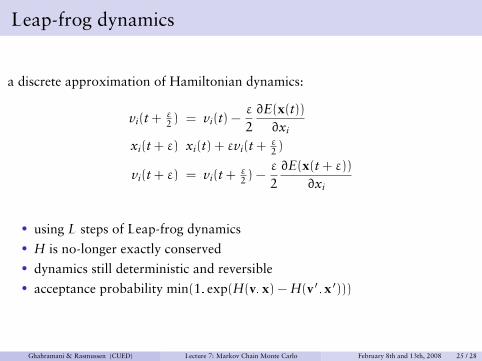
Leap-frog dynamics

a discrete approximation of Hamiltonian dynamics:

vi(t + ε2 ) = vi(t) −

ε

2∂E(x(t))

∂xi

xi(t + ε) xi(t) + εvi(t + ε2 )

vi(t + ε) = vi(t + ε2 ) −

ε

2∂E(x(t + ε))

∂xi

• using L steps of Leap-frog dynamics• H is no-longer exactly conserved• dynamics still deterministic and reversible• acceptance probability min(1, exp(H(v, x) − H(v ′, x ′)))


Hybrid Monte Carlo avoids random walks

The advantage of introducing velocity variables is that random walks are avoided.


Summary

Rejection and Importance sampling are based on independent samples from q(x).

These methods are not suitable for high dimensional problems.

The Metropolis method, does not give independent samples, but can be usedsuccessfully in high dimensions.

Gibbs sampling is used extensively in practice.

• parameter-free• requires simple conditional distributions

Hybrid Monte Carlo is used extensively in continuous systems

• avoids random walks• requires setting of ε and L.


Monte Carlo in Practice

Although very general, and can be applied in systems with 1000’s of variables.

Care must be taken when using MCMC

• high dependency between variables may cause slow exploration• how long does ’burn-in’ take?• how correlated are the samples generated?• slow exploration may be hard to detect – but you might not be getting

the right answer• diagnosing a convergence problem may be difficult• curing a convergence problem may be even more difficult


Lecture 7: Markov Chain Monte Carlo

Documents

Transcript of Lecture 7: Markov Chain Monte Carlo